Structured Compression by Weight Encryption
for Unstructured Pruning and Quantization
Abstract
Model compression techniques, such as pruning and quantization, are becoming increasingly important to reduce the memory footprints and the amount of computations. Despite model size reduction, achieving performance enhancement on devices is, however, still challenging mainly due to the irregular representations of sparse matrix formats. This paper proposes a new weight representation scheme for Sparse Quantized Neural Networks, specifically achieved by fine-grained and unstructured pruning method. The representation is encrypted in a structured regular format, which can be efficiently decoded through XOR-gate network during inference in a parallel manner. We demonstrate various deep learning models that can be compressed and represented by our proposed format with fixed and high compression ratio. For example, for fully-connected layers of AlexNet on ImageNet dataset, we can represent the sparse weights by only 0.28 bits/weight for 1-bit quantization and 91% pruning rate with a fixed decoding rate and full memory bandwidth usage. Decoding through XOR-gate network can be performed without any model accuracy degradation with additional patch data associated with small overhead.
1 Introduction
Deep neural networks (DNNs) are evolving to solve increasingly complex and varied tasks with dramatically growing data size deeplearningbook. As a result, the growth rate of model sizes for recent DNNs leads to slower response times and higher power consumption during inference EIE. To mitigate such concerns, model compression techniques have been introduced to significantly reduce model size of DNNs while maintaining reasonable model accuracy.


It is well known that DNNs are designed to be over-parameterized in order to ease local minima exploration denil2013predicting; frankle2018lottery. Thus, various model compression techniques have been proposed for high-performance and/or low-power inference. For example, pruning techniques remove redundant weights (to zero) without compromising accuracy optimalbrain, in order to achieve memory and computation reduction on devices SHan_2015; sparseVD; suyog_prune; DeepTwist. As another model compression technique, non-zero weights can be quantized to fewer bits with comparable model accuracy of full-precision parameters, as discussed in binaryconnect; rastegariECCV16; Hubara2016; xu2018alternating.
To achieve even higher compression ratios, pruning and quantization can be combined to form Sparse Quantized Neural Networks (SQNNs). Intuitively, quantization can leverage parameter pruning since pruning reduces the number of weights to be quantized and quantization loss decreases accordingly quant_lee. Deep compression deepcompression, ternary weight networks (TWN) TWN, trained ternary quantization (TTQ) ternary2017, and viterbi-based compression viterbi_quantized; lee2018viterbibased represent recent efforts to synergistically combine pruning and quantization.
To benefit from sparsity, it is important to (1) represent pruned models in a format with small memory footprint and (2) implement fast computations with sparse matrices as input operands. Even if reduced SQNNs can be generated with a high pruning rate, it is challenging to gain performance enhancement without an inherently parallel sparse-matrix decoding process during inference. To illustrate such a challenge, Figure 1 presents DRAM bandwidth, the number of transactions, and execution time of a matrix multiplication using one random sparse matrix (following CSR format) and a random dense matrix on NVIDIA Tesla V100 (supported by CUDA 9.1). Because of unbalanced workloads (note that pruning each weight is a somewhat independent and random operation) and additional data for index, sparse matrix computations using CSR format do not offer performance gain as much as sparsity. Moreover, if pruning rate is not high enough, sparse matrix operations can be even slower than dense matrix operations.
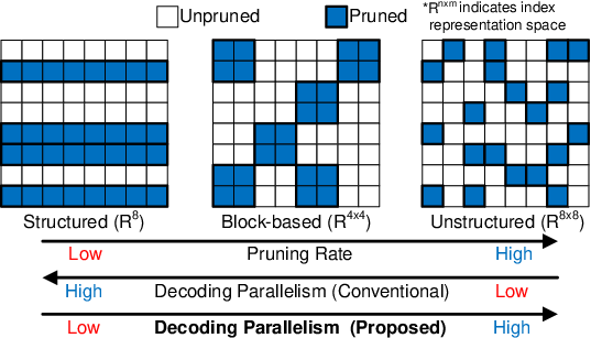
As such, structured and blocked-based pruning techniques li2016pruning; anwar2017structured; scalpel2017; he2017channel; ye2018rethinking for DNNs have been proposed to accelerate decoding of sparse matrices using reduced indexing space, as Figure 2 shows. However, coarse-grained pruning associated with reduced indexing space exhibits relatively lower pruning rates compared to unstructured pruning mao2017exploring, which masks weights with fine-grained granularity. In conventional sparse matrix formats representing unstructured pruning (i.e., random weights can be pruned), decoding time can vastly differ if decoding processes are conducted in different blocks simultaneously, as shown in the conventional approach of Figure 3.
To enable inherently parallel computations using sparse matrices, this paper proposes a new sparse format. Our main objective is to remove all pruned weights such that the resulting compression ratio tracks the pruning rate, while maintaining a regular format. Interestingly, in VLSI testing, proposals for test-data compression have been developed from similar observations, i.e., there are lots of don’t care bits (= pruned weights in the case of model compression) and the locations of such don’t care bits seem to be random survey_test (the locations of unstructurally pruned weights also seem to be random). We adopt XOR-gate network, previously used for test-data compression, to decode the compressed bits in a fixed rate during inference, as shown in Figure 3. XOR-gate network is small enough such that we can embed multiple XOR-gate networks to fully utilize memory bandwidth and decode many sparse blocks concurrently. Correspondingly, we propose an algorithm to find encrypted and compressed data to be fed into XOR-gate network as inputs.
| CSR Format | Viterbi-based Compr. | Proposed | |
| Encryption | No | Yes | Yes |
| Load Balance | Uneven | Even | Even |
| Decoding Rate | Variable | Fixed | Fixed |
| Parallelism Limited by | Uneven Sparsity | Number of Decoders | Number of Decoders |
| Memory Access Pattern | Irregular (Gather-Scatter) | Regular | Regular |
| Compressed Memory Bandwidth | Depends on on-chip Buffer Structure | 1 bit/decoder | Multi-bits/decoder |
| HW Resource for a Decoder | Large Buffer to improve load balance | XOR gates and Flip-Flops | XOR gates only |
2 Related Works and Comparison
In this section, we introduce two previous approaches to represent sparse matrices. Table 1 describes CSR format, Viterbi-based index format, and our proposed method.
Compressed Sparse Row (CSR): Deep compression deepcompression utilizes the Compressed Sparse Row (CSR) format to reduce memory footprint on devices. Unfortunately, CSR formats (including blocked CSR) present irregular data structures not readily supported by highly parallel computing systems such as CPUs and GPUs lee2018viterbibased. Due to uneven sparsity among rows, computation time of algorithms based on CSR is limited by the least sparse row zhou2018cambricon, as illustrated in Figure 3. Although EIE suggested hardware supports via a large buffer to improve load balancing, performance is still determined by the lowest pruning rate of a particular row. In contrast, our scheme provides a perfectly structured format of weights after compression such that high parallelism is maintained.
Viterbi Approaches: Viterbi-based compression lee2018viterbibased; viterbi_quantized attempts to compress pruning-index data and quantized weights with a fixed compression ratio using don’t care bits, similar to our approach. Quantized weights can be compressed by using the Viterbi algorithm to obtain a sequence of inputs to be fed into Viterbi encoders (one bit per cycle). Because only one bit is accepted for each Viterbi encoder, only an integer number (=number of Viterbi encoder outputs) is permitted as a compression ratio, while our proposed scheme allows any rational numbers.
Because only one bit is used as inputs for Viterbi encoders, Viterbi-based approaches require large hardware resources. For example, if a memory allows 1024 bits per cycle of bandwidth, then 1024 Viterbi encoders are required, where each Viterbi encoder entails multiple Flip-Flops to support sequence detection. On the other hand, our proposed scheme is resource-efficient to support large memory bandwidth because Flip-Flops are unnecessary.
3 Proposed Weight Representation for Structured Compression
Test-data compression usually generates random numbers as outputs using the input data as seed values. The outputs (test data containing don’t care bits) can be compressed successfully if such outputs can be generated by the random number generator using at least one particular input seed data (which is the compressed test data). It is well known that memory reduction can be as high as the portion of don’t care bits Orailoglu; survey_test if randomness is good enough. Test data compression and SQNNs with fine-grained pruning share the following properties: 1) Parameter pruning induces don’t care values as much as pruning rates and 2) If a weight is unpruned, then each quantization bit is assigned to 0 or 1 with equal probability viterbi_quantized. In this section, we propose a new weight representation method exploiting such shared properties while fitting high memory bandwidth requirements and lossless compression to maintain accuracy.
3.1 Encryption and Decryption

We use an XOR-gate network as a random number generator due to its simple design and strong compression capability (such a generator is not desirable for test-data compression because it requires too many input bits). Suppose that a real-number weight matrix is quantized to be binary matrices () with as the number of bits for quantization. As the first step of our encryption algorithm, we reshape each binary matrix to be a 1D vector, which is then evenly divided into smaller vector sequences of size. Then, each of the evenly divided vectors, , including don’t care bits is encrypted to be a small vector (of size) without any don’t care bits. Through the XOR-gate network, each encrypted vector is decrypted to be original bits consisting of correct care bits and randomly filled don’t care bits with respect to . Figure 4 illustrates encryption and decryption procedure examples using a weight matrix. A 4D tensor (e.g. conv layers) can also be encrypted through the same procedures after flattening.
The structure of XOR-gate network is fixed during the entire process and, as depicted in Figure 5, can be described as a binary matrix over Galois Field with two elements, , using the connectivity information between the input vector (compressed and encrypted weights) and . Note that is pre-determined and designed in a way that each element is randomly assigned to 0 or 1 with the same probability.

We intend to generate a random output vector using a seed vector while targeting as many care bits of as possible. In order to increase the number of successfully matched care bits, XOR-gate network should be able to generate various random outputs. In other words, when the sizes of a seed vector and an output vector are given as and respectively, all possible outputs need to be well distributed in solution space.
Before discussing how to choose and , let us first study how to find a seed vector , given . As shown in Figure 5, the overall operation can be expressed by linear equations over . Note that linear equations associated with don’t care bits in can be ignored, because decryption through XOR-gate network can produce any bits in the locations of don’t care bits. By deleting unnecessary linear equations, the original equations can be reduced as below:
| (1) |
- •
is a set of indices indicating care bits of each vector ().
- •
For example, since only 4 care bits () exist in Figure 5, the (84) matrix is reduced to a (44) matrix, , by removing 1st, 2nd, 6th, and 8th rows.
Given the pruning rate , contains care bits on average. Assuming that equations are independent and non-trivial, the required number of seed inputs () can be as small as , wherein the compression ratio becomes . As a result, higher pruning rates lead to higher compression ratios. However, note that the linear equations may not have a corresponding solution when there are too many ‘local’ care bits or there are conflicting equations for a given vector .
3.2 Extra Patches for Lossless Compression
In order to keep our proposed SQNNs representation lossless, we add extra bits to correct unavoidable errors, i.e., patching. An unsolvable linear equation implies that the XOR random number generator cannot produce one or more matched care bits of . To resolve such an occasion, we can replace one or more care bits of with don’t care bits to remove conflicting linear equations, as depicted in Figure 6. We record the locations of replacements as which can be used to recover the original care bits of by flipping the corresponding bits during decryption. For every , indicates the number of replacements for each . Since is always scanned prior to decryption using , the same number of bits is reserved to represent for all encrypted vectors in order to maintain a regular compressed format. On the other hand, the size of can be different for each (overall parallelism is not disrupted by different sizes as flipping occurs infrequently).
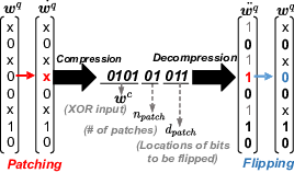
At the expense of and , our compression technique can reproduce all care bits of and, therefore, does not affect accuracy of DNN models and obviates retraining. In sum, the compressed format includes 1) () encrypted from a quantized weight matrix through , 2) , and 3) . Hence, the resulting compression ratio is
| (2) |
where is the th and = . Improving is enabled by increasing and decreasing the amount of patches. We introduce a heuristic patch-searching algorithm to reduce the number of patches while also optimizing and .
3.3 Experiments Using Synthetic Data


An exhaustive search of patches requires exponential-time complexity even though such a method minimizes the number of patches. Algorithm 1 is a heuristic algorithm to search encrypted bits including and for in . The algorithm incrementally enlarges the reduced linear equation by including a care bit only when the enlarged equation is still solvable. Note that make_rref() in Algorithm 1 generates a reduced row-echelon form to quickly verify that the linear equations are solvable. If adding a certain care bit makes the equations unsolvable, then a don’t care bit takes its place, and and are updated accordingly. Although Algorithm 1 yields more replacement of care bits than an exhaustive search (by up to 10% from our extensive experiments), our simple algorithm has time complexity of , which is much faster.
To investigate the compression capability of our proposed scheme, we evaluate a large random weight matrix of 10,000 elements where each element becomes a don’t care bit with the probability of 0.9 (=sparsity or pruning rate). If an element is a care bit, then a 0 or 1 is assigned with the same probability. Notice that randomness of locations in don’t care bits is a feature of fine-grained pruning methods and assignment of 0 or 1 to weights with the same probability is obtainable using well-balanced quantization techniques viterbi_quantized; lee2018viterbibased.
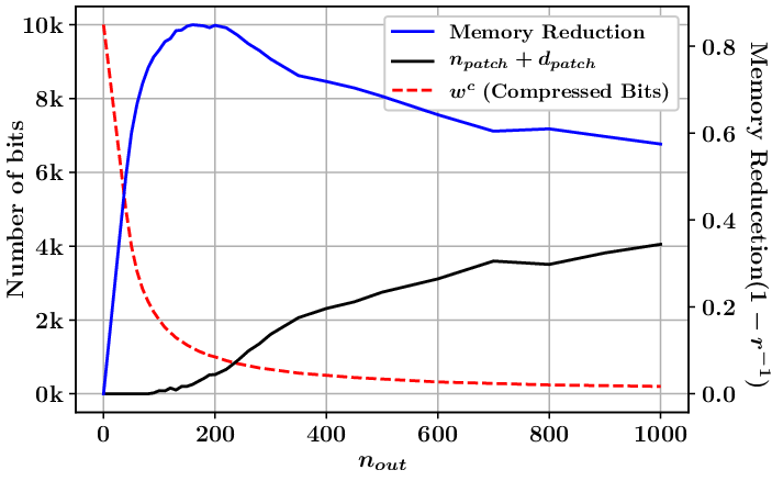
When is fixed, the optimal maximizes the memory reduction offered by Algorithm 1. Figure 7 plots the corresponding memory reduction (=) from on the right axis and the amount of and + on the left axis across a range of values when . From Figure 7, it is clear that there exists a trade-off between the size of and the sizes of and . Increasing rapidly reduces while and grow gradually. The highest memory reduction () is achieved when is almost 200, which agrees with the observation that maximum compression is constrained by the relative number of care bits survey_test. Consequently, the resulting compression ratio approaches .
Given the relationship above, we can now optimize . Figure 8 compares memory reduction for various across different values of . The resulting trend suggests that higher yields more memory reduction. This is because increasing the number of bits used as seed values for the XOR-gate random number generator enables a larger solution space and, as a result, fewer are needed as increases. The large solution space is especially useful when don’t care bits are not evenly distributed throughout . Lastly, is constrained by the maximum computation time available to run Algorithm 1.
Figure 9 presents the relationship between pruning rate and memory reduction when and sweeping . Since high pruning rates translate to fewer care bits and relatively fewer , Figure 9 confirms that memory reduction reaches as increases. In other words, maximizing pruning rate is key to compressing quantized weights with high compression ratio. In comparison, ternary quantization usually induces a lower pruning rate ternary2017; TWN. Our proposed representation is best implemented by pruning first to maximize pruning rate and then quantizing the weights.
4 Experiments on various SQNNs
| Target Model | Pre-trained | Pruning and Quantization | ||||
| Model | DataSet | Size | Acc. | -bit | Acc. | |
| LeNet5 (FC1) | MNIST | 800500 | 99.1% | 0.95 | 1-bit | 99.1% |
| AlexNet (FC5, FC6) | ImageNet | 9K4K, 4K4K | 57.6% (T1) | 0.91 | 1-bit | 55.9% (T1) |
| ResNet32 (Conv Layers) | CIFAR10 | 460.76K | 92.5% | 0.70 | 2-bit | 91.6% |
| LSTM | PTB | 6.41M | 89.6 PPW | 0.60 | 2-bit | 93.9 PPW |

In this section, we show experimental results of the proposed representation for four popular datasets: MNIST, ImageNet imagenet, CIFAR10 cifar10, and Penn Tree Bank ptb. Though the compression ratio ideally reaches , the actual results may not, because don’t care bits can be less evenly distributed than the synthetic data we used for Section 3.3. Hence, we suggest several additional techniques in this section to handle uneven distributions.
Weights are pruned by the mask layer generated by binary-index matrix factorization ourBMF after pre-training, and then retrained. Quantization is performed by following the technique proposed in DeepTwist and efficient_quant, where quantization-aware optimization is performed based on the quantization method from xu2018alternating. The number of bits per weight required by our method is compared with the case of -bit quantization with an additional 1-bit indicating pruning index (e.g., ternary quantization consists of 1-bit quantization and 1-bit pruning indication per weight).
We first tested our representation using the LeNet-5 model on MNIST. LeNet-5 consists of two convolutional layers and two fully-connected layers SHan_2015; DeepTwist. Since the FC1 layer dominates the memory footprint (93%), we focus only on the FC1 layer whose parameters can be pruned by 95%. With our proposed method, the FC1 layer is effectively represented by only 0.19 bits per weight, which is smaller than ternary quantization, as Figure 10 shows. We also tested our proposed compression techniques on large-scale models and datasets, namely, AlexNet alexnet on the ImageNet dataset. We focused on compressing FC5 and FC6 fully-connected layers occupying 90% of the total model size for AlexNet. Both layers are pruned by a pruning rate of 91% SHan_2015 using binary-index matrix factorization ourBMF and compressed by 1-bit quantization. The high pruning rate lets us compress the quantized weights by . Overall, FC5 and FC6 layers for AlexNet require only 0.28 bits per weight, which is substantially less than 2 bits per weight required by ternary quantization.
We further verify our compression techniques using ResNet32 resnet on the CIFAR10 dataset with a baseline accuracy of 92.5%. The model is pruned and quantized to 2 bits, reaching 91.6% accuracy after retraining. Further compression with our proposed SQNN format yields 1.22 bits per weight, while 3 bits would be required without our proposed compression techniques.
Additionally, an RNN model with one LSTM layer of size 300 xu2018alternating on the PTB dataset, with performance measured by using Perplexity Per Word, is compressed by our representation. Following our proposed representation scheme along with pruning and 2-bit quantization, such PTB LSTM model requires only 1.67 bits per weight.
For various types of layers, our proposed technique, supported by weight sparsity, provides additional compression over ternary quantization. Compression ratios can be further improved by using more advanced pruning and quantization methods (e.g., HitNet; DNS) since the principles of our compression methods do not rely on the specific pruning and quantization methods used.
5 Discussion
5.1 Variation on Execution Time
While decryption process through XOR-gate network provides a fixed output rate (thus, high parallelism), if all mismatched bits are supposed to be corrected by patches, then entire decoding (including decryption and patch correction) may result in variation in execution time due to irregular patch size. In order to mitigate variation in patch process, we first assume that patch data structure is decoupled from encrypted weights such that is given as a stream data to be stored into buffers in a fixed rate. Then, for each XOR decryption cycle, as much as is read from buffers and used to fix XOR outputs. In Figure 11, is stored into or loaded from FIFO buffers when the number of FIFO banks is . If is needed, FIFO buffers deliver to patch process logic while available throughput for load/store is determined by the number of FIFO banks. Decoding process can be stalled when the FIFO is either full or empty if temporal consumption rate is too low or too high.
Figure 12 presents relative execution time using CSR format or the proposed scheme with different configurations. FIFO size can be small enough (say, 256 entries) to tolerate temporal high peak usage. Hence, in Figure 12, stalls in the proposed scheme are due to high throughput demands along with large . Note that CSR format yields high variations in execution time because each row exhibits various numbers of unpruned weights. On the other hand, in the case of the proposed scheme, increasing (at the cost of additional hardware design) enhances throughput, and thus, reduces the number of stalls incurred by limited bandwidth of FIFOs. In sum, reasonable size significantly reduces execution time variations, which has been a major bottleneck in implementing fine-grained pruning schemes, as demonstrated in Figure 1.


5.2 Practical Techniques to Reduce
If is large enough, patching overhead is not supposed to disrupt the parallel decoding, ideally. However, even for large , if the nonuniformity of pruning rates is observed over a wide range within a matrix, may considerably increase. Large , then, leads to not only degraded compression ratio compared with synthetic data experiments, but also deteriorated parallelism in the decoding process. The following techniques can be considered to reduce .
Blocked Assignment: The compression ratio in the Eq. (8) of Section 3.2 is affected by the maximum of . Note that a particular vector may have an exceptionally large number of care bits. In such a case, even if a quantized matrix consists of mostly don’t care bits and few patches are needed, all of the compressed vectors must employ a large number of bits to track the number of patches. To mitigate such a problem and enhance the compression ratio , we divide a binary matrix into several blocks, and then is obtained in each block independently. Different is assigned to each block to reduce the overall data size.
Minimizing for Small : One simple patch-minimizing algorithm is to list all possible inputs (for ) and corresponding outputs through on memory and find a particular that minimizes the number of patches. At the cost of high space complexity and memory consumption, such an exhaustive optimization guarantees minimized . below 30 is a practical value.
6 Conclusion
This paper proposes a compressed representation for Sparse Quantized Neural Networks based on an idea used for test-data compression. Through XOR-gate network and solving linear equations, we can remove most don’t care bits and a quantized model is further compressed by sparsity. Since our representation provides a regular compressed-weight format with fixed and high compression ratios, SQNNs enable not only memory footprint reduction but also inference performance improvement due to inherently parallelizable computations.
References
- (1) Daehyun Ahn, Dongsoo Lee, Taesu Kim, and Jae-Joon Kim. Double Viterbi: Weight encoding for high compression ratio and fast on-chip reconstruction for deep neural network. In International Conference on Learning Representations (ICLR), 2019.
- (2) Sajid Anwar, Kyuyeon Hwang, and Wonyong Sung. Structured pruning of deep convolutional neural networks. ACM Journal on Emerging Technologies in Computing Systems (JETC), 13(3):32, 2017.
- (3) Ismet Bayraktaroglu and Alex Orailoglu. Test volume and application time reduction through scan chain concealment. In Proceedings of the 38th Annual Design Automation Conference, 2001.
- (4) Matthieu Courbariaux, Yoshua Bengio, and Jean-Pierre David. BinaryConnect: Training deep neural networks with binary weights during propagations. In Advances in Neural Information Processing Systems, pages 3123–3131, 2015.
- (5) Misha Denil, Babak Shakibi, Laurent Dinh, Nando De Freitas, et al. Predicting parameters in deep learning. In Advances in neural information processing systems, pages 2148–2156, 2013.
- (6) Jonathan Frankle and Michael Carbin. The lottery ticket hypothesis: Finding sparse, trainable neural networks. arXiv preprint arXiv:1803.03635, 2018.
- (7) Ian Goodfellow, Yoshua Bengio, and Aaron Courville. Deep Learning. MIT Press, 2016. http://www.deeplearningbook.org.
- (8) Yiwen Guo, Anbang Yao, and Yurong Chen. Dynamic network surgery for efficient DNNs. In Advances in Neural Information Processing Systems, 2016.
- (9) Song Han, Xingyu Liu, Huizi Mao, Jing Pu, Ardavan Pedram, Mark A. Horowitz, and William J. Dally. EIE: efficient inference engine on compressed deep neural network. In Proceedings of the 43rd International Symposium on Computer Architecture, pages 243–254, 2016.
- (10) Song Han, Huizi Mao, and William J. Dally. Deep compression: Compressing deep neural networks with pruning, trained quantization and Huffman coding. In International Conference on Learning Representations (ICLR), 2016.
- (11) Song Han, Jeff Pool, John Tran, and William J. Dally. Learning both weights and connections for efficient neural networks. In Advances in Neural Information Processing Systems, pages 1135–1143, 2015.
- (12) Kaiming He, Xiangyu Zhang, Shaoqing Ren, and Jian Sun. Deep residual learning for image recognition. 2016 IEEE Conference on Computer Vision and Pattern Recognition (CVPR), pages 770–778, 2016.
- (13) Yihui He, Xiangyu Zhang, and Jian Sun. Channel pruning for accelerating very deep neural networks. In Proceedings of the IEEE International Conference on Computer Vision, pages 1389–1397, 2017.
- (14) Itay Hubara, Matthieu Courbariaux, Daniel Soudry, Ran El-Yaniv, and Yoshua Bengio. Quantized neural networks: training neural networks with low precision weights and activations. arXiv:1609.07061, 2016.
- (15) Parichay Kapoor, Dongsoo Lee, Byeongwook Kim, and Saehyung Lee. Computation-efficient quantization method for deep neural networks, 2019.
- (16) Alex Krizhevsky. Learning multiple layers of features from tiny images. Technical report, 2009.
- (17) Alex Krizhevsky, Ilya Sutskever, and Geoffrey E Hinton. Imagenet classification with deep convolutional neural networks. In F. Pereira, C. J. C. Burges, L. Bottou, and K. Q. Weinberger, editors, Advances in Neural Information Processing Systems 25, pages 1097–1105. Curran Associates, Inc., 2012.
- (18) Yann LeCun, John S. Denker, and Sara A. Solla. Optimal brain damage. In Advances in Neural Information Processing Systems, pages 598–605, 1990.
- (19) Dongsoo Lee, Daehyun Ahn, Taesu Kim, Pierce I. Chuang, and Jae-Joon Kim. Viterbi-based pruning for sparse matrix with fixed and high index compression ratio. In International Conference on Learning Representations (ICLR), 2018.
- (20) Dongsoo Lee, Parichay Kapoor, and Byeongwook Kim. Deeptwist: Learning model compression via occasional weight distortion. arXiv:1810.12823, 2018.
- (21) Dongsoo Lee and Byeongwook Kim. Retraining-based iterative weight quantization for deep neural networks. arXiv:1805.11233, 2018.
- (22) Dongsoo Lee, Se Jung Kwon, Parichay Kapoor, Byeongwook Kim, and Gu-Yeon Wei. Network pruning for low-rank binary indexing. arXiv:1905.05686, 2019.
- (23) Fengfu Li and Bin Liu. Ternary weight networks. arXiv:1605.04711, 2016.
- (24) Hao Li, Asim Kadav, Igor Durdanovic, Hanan Samet, and Hans Peter Graf. Pruning filters for efficient convnets. In International Conference on Learning Representations, 2017.
- (25) Huizi Mao, Song Han, Jeff Pool, Wenshuo Li, Xingyu Liu, Yu Wang, and William J Dally. Exploring the regularity of sparse structure in convolutional neural networks. arXiv preprint arXiv:1705.08922, 2017.
- (26) Mitchell Marcus, Grace Kim, Mary Ann Marcinkiewicz, Robert MacIntyre, Ann Bies, Mark Ferguson, Karen Katz, and Britta Schasberger. The penn treebank: Annotating predicate argument structure. In Proceedings of the Workshop on Human Language Technology, HLT ’94, pages 114–119, Stroudsburg, PA, USA, 1994. Association for Computational Linguistics.
- (27) Dmitry Molchanov, Arsenii Ashukha, and Dmitry P. Vetrov. Variational dropout sparsifies deep neural networks. In International Conference on Machine Learning (ICML), pages 2498–2507, 2017.
- (28) Mohammad Rastegari, Vicente Ordonez, Joseph Redmon, and Ali Farhadi. XNOR-Net: Imagenet classification using binary convolutional neural networks. In ECCV, 2016.
- (29) Olga Russakovsky, Jia Deng, Hao Su, Jonathan Krause, Sanjeev Satheesh, Sean Ma, Zhiheng Huang, Andrej Karpathy, Aditya Khosla, Michael Bernstein, Alexander C. Berg, and Li Fei-Fei. ImageNet Large Scale Visual Recognition Challenge. International Journal of Computer Vision (IJCV), 115(3):211–252, 2015.
- (30) Nur A. Touba. Survey of test vector compression techniques. IEEE Design & Test of Computers, 23:294–303, 2006.
- (31) Peiqi Wang, Xinfeng Xie, Lei Deng, Guoqi Li, Dongsheng Wang, and Yuan Xie. HitNet: Hybrid ternary recurrent neural network. In Advances in Neural Information Processing Systems, 2018.
- (32) Chen Xu, Jianqiang Yao, Zhouchen Lin, Wenwu Ou, Yuanbin Cao, Zhirong Wang, and Hongbin Zha. Alternating multi-bit quantization for recurrent neural networks. In International Conference on Learning Representations (ICLR), 2018.
- (33) Jianbo Ye, Xin Lu, Zhe Lin, and James Z Wang. Rethinking the smaller-norm-less-informative assumption in channel pruning of convolution layers. arXiv preprint arXiv:1802.00124, 2018.
- (34) Jiecao Yu, Andrew Lukefahr, David Palframan, Ganesh Dasika, Reetuparna Das, and Scott Mahlke. Scalpel: Customizing DNN pruning to the underlying hardware parallelism. In Proceedings of the 44th Annual International Symposium on Computer Architecture, pages 548–560, 2017.
- (35) Xuda Zhou, Zidong Du, Qi Guo, Shaoli Liu, Chengsi Liu, Chao Wang, Xuehai Zhou, Ling Li, Tianshi Chen, and Yunji Chen. Cambricon-s: Addressing irregularity in sparse neural networks through a cooperative software/hardware approach. In 2018 51st Annual IEEE/ACM International Symposium on Microarchitecture (MICRO), pages 15–28. IEEE, 2018.
- (36) Chenzhuo Zhu, Song Han, Huizi Mao, and William J. Dally. Trained ternary quantization. In International Conference on Learning Representations (ICLR), 2017.
- (37) Michael Zhu and Suyog Gupta. To prune, or not to prune: exploring the efficacy of pruning for model compression. CoRR, abs/1710.01878, 2017.