A Trilinear Immersed Finite Element Method
for Solving Elliptic Interface
Problems
Abstract
This article presents an immersed finite element (IFE) method for solving the typical three-dimensional second order elliptic interface problem with an interface-independent Cartesian mesh. The local IFE space on each interface element consists of piecewise trilinear polynomials which are constructed by extending polynomials from one subelement to the whole element according to the jump conditions of the interface problem. In this space, the IFE shape functions with the Lagrange degrees of freedom can always be constructed regardless of interface location and discontinuous coefficients. The proposed IFE space is proven to have the optimal approximation capabilities to the functions satisfying the jump conditions. A group of numerical examples with representative interface geometries are presented to demonstrate features of the proposed IFE method.
1 Introduction
Let be a domain, and, without loss of generality, we assume that is separated into two subdomains and by a closed interface surface . These subdomains contain different materials identified by a piecewise constant parameter discontinuous across the interface , i.e.,
We consider the following interface problem of the elliptic type on :
| (1.1a) | ||||
| (1.1b) | ||||
| (1.1c) | ||||
| (1.1d) | ||||
where is the normal vector to . For simplicity, we denote , , in the rest of this article.
The elliptic interface problem (1.1) has wide applications in science and engineering such as inverse problems [26, 35, 49], fluid dynamics [38, 41], biomolecular electrostatics [21, 53], plasma simulation [8, 34], to name just a few. Traditional finite element methods can be applied to solve this interface problem based on an interface-fitted mesh [6, 13, 54]. However, when the interface has complex geometry, for example the material interface in biomedical images [4, 49] and geophysical images [16] in the 3-D case, it is a time-consuming and non-trivial process to generate a high-quality interface-fitted mesh to resolve the interface geometry. And this mesh generation issue will become more severe if the interface changes its shape or moves in computation. Recently, a new finite element method based on a semi-structured mesh was proposed in [12] where the interface geometry is fitted by a local Delaunay triangulation on interface elements of a pre-generated background Cartesian mesh.
Alternatively, methods that can solve the interface problem (1.1) on a mesh independent of the interface geometry, referred as the unfitted mesh methods, have drawn attention from researchers. Methods in this category can be roughly categorized into two groups: modify computation scheme around the interface or modify finite element functions on interface elements. Examples in the first group are the immersed interface methods (IIM) [37, 40] in the finite difference context and the CutFEM [11, 31] based on the finite element scheme. Methods in the second group can be found for the multiscale finite element methods [14, 19], the extended finite element methods [17, 47], the partition of unity methods [45, 48] and the immersed finite element (IFE) methods to be discussed in this article. We note that some of these methods may actually involve both the two types of modifications.
The key idea in the IFE methods is to use piecewise polynomials constructed according to the jump conditions on interface elements, i.e., the Hsieh-Clough-Tocher [9, 15] type macro elements, to capture the jump behaviors across the interface, while standard polynomials are used over non-interface elements. In addition to the optimal convergence rate the IFE method can achieve on a unfitted mesh, it can also keep the number and location of degrees of freedom isomorphic to the standard finite element method defined on the same mesh. And this feature is advantageous when dealing with moving interface problems for which we refer readers to [3, 7, 26, 33, 42].
In this work, we discuss a trilinear IFE method on a highly structured mesh (Cartesian mesh) for solving the interface problem (1.1) with optimal accuracy. Our research presented here is motivated by real-world problems. For example, in plasma simulations in composite materials by the particle-in-cell (PIC) code [8, 34], many macro-particles modeling a plasma in the self-consistent electromagnetic field have to be traced and located on elements in a mesh iteratively during their motion in order to perform the particle-mesh interpolation procedure; therefore a structure mesh is preferred to a unstructured mesh because of the computational cost in search. As an another example, in electroencephalography, a background Cartesian mesh for a head model can be constructed by the pixels of magnetic resonance images (MRIs) [49] for finite element computation. We refer readers to [36, 49, 51] for the applications of IFE methods in these fields.
Although many works on the 2-D IFE methods have appeared in the literature, such as [22, 23, 25, 27, 28, 32, 43, 44] for theoretical analysis and [2, 3, 7, 26, 51] for applications, to name just a few, the study on the 3-D case is relatively sparse, see [36] for a linear IFE method and [49] for a trilinear IFE method. Even though the research reported here is within the direction of that in [49], but our work has three distinct new contributions. The first one is a group of detailed geometric estimates for a suitable linear approximation of the interface surface on each interface element. In particular, we introduce a maximal angle condition for constructing such a special linear approximation to the interface surface with optimal accuracy in terms of the surface curvature and mesh size. Both the theoretical analysis and numerical experiments indicate that this maximal angle condition and the resulted geometric properties are the foundation of the optimal approximation capabilities for the proposed IFE spaces. We also believe these fundamental geometric estimates can be useful for other unfitted mesh methods. Secondly, on interface elements, we construct local IFE spaces by extending trilinear polynomials from one subelement to another through a discretized extension operator designed according to the jump conditions across the interface. IFE shape functions with some desirable features, such as the Lagrange type degrees of freedom, can be readily constructed from this space and their existence is guaranteed completely independent of the interface location and coefficients . Moreover, the extension operator enables us to establish the optimal approximation capabilities for the proposed IFE spaces. To the best of our knowledge, this is the first work for 3-D IFE methods covering both the development and basic analysis. We highlight that the proposed construction and analysis techniques can be readily extendable to IFE methods on unstructured unfitted meshes for solving the elliptic interface problems.
This article consists of four additional sections. In the next section, we establish a group of fundamental geometric estimates. In Section 3, we develop the trilinear IFE space and construct the Lagrange IFE shape functions. In Section 4, we analyze the approximation capabilities of the proposed IFE space. In the last section, we present a group of numerical examples with representative geometries of the interface surface to demonstrate the features of the proposed IFE method.
2 Some Geometries of Interface Elements
In this section, we present some geometric properties related to the interface surface and interface elements. These properties are fundamental for both the construction of the IFE spaces to be proposed and the related error analysis.
Throughout this article, we assume the bounded domain is a union of finitely many rectangular parallelepipeds, and let be a Cartesian mesh of the domain with the maximum length of edge . We let and be the collection of faces and edges in this mesh . We call an element an interface element if ; otherwise, we call it a non-interface element. Similarly, we can define the interface faces and edges. Furthermore, we use // and // to denote the collection of interface and non-interface elements/faces/edges, respectively.
Given each measurable subset , let be the standard Sobolev spaces on with the Sobolev norm and the semi-norm , for . The corresponding Hilbert space is associated with the norm and semi-norm . In the case , we define the splitting Hilbert space
| (2.1) |
where the definition implicitly implies the involved traces on are well defined, with the associated norms
Furthermore, for each interface element, we define its patch as
| (2.2) |
We begin by recalling the definition and existence of a so called -tubular neighborhood of the smooth interface surface which are based on the following Lemma from [20].
Lemma 2.1 (-tubular neighborhood).
Given a smooth compact surface in , for each , let be a segment with the length centered at and perpendicular to . Then, there exists a positive such that for any .
The -tubular neighborhood of is defined as the set . The existence of the -tubular neighborhood of a smooth surface is given in [20]. Define as the largest such that Lemma 2.1 holds, and this positive number is referred as the reach of the surface in some literature [46]. In the following discussion, we assume that
- (H1)
.
- (H2)
The interface surface can not intersect any edge at more than one point.
- (H3)
The interface surface can not intersect the boundary of any face at more than two points.
We note that a similar assumption as (H1) about the -tubular neighborhood has been used in a 2D unfitted mesh method [30]. And the assumptions (H2) and (H3) basically mean the interface surface is resolved enough by the unfitted mesh, and these assumptions have been used in many works on unfitted meshes such as [11, 23, 31, 36]. These assumptions can be satisfied when the interface surface is flat enough locally inside each interface element which holds in general when the mesh size is sufficiently small. In particular, for each interface element , (H1) guarantees that its patch is inside the -tubular neighborhood of the interface surface.
Based on the assumptions (H2) and (H3), an interface surface can only intersect a cubic interface element with at least three faces but no more than six faces. Therefore, by considering rotations, we classify the interface element configuration according to the number of interface faces of : only one possible configuration for three interface faces as shown by Case 1 in Figure 2.1, two possible configurations for four interface faces as shown by Case 2 and Case3 in Figure 2.1, one possible configuration for five interface faces as shown by Case 4 in Figure 2.1 and one possible configuration for six interface faces as shown by Case 5 in Figure 2.1. Moreover, it can be considered as certain limit situations of those interface configurations in Figure 2.1 when some vertices of are on the interface surface; and our construction and analysis techniques developed below are readily extended to handle these situations. Therefore, in the following discussion, for the simplicity of presentations, we only discuss these five interface element configurations. This classification approach can be easily implemented to determine which configuration an interface element belongs to by counting the interface faces and location of vertices relative to the interface.


The fundamental idea of the IFE methods is the employment of piecewise polynomials constructed on interface elements to satisfy the jump conditions in a certain approximate sense. On each interface element , a 2D IFE function is a piecewise polynomial defined according to the two subelements formed by the straight line connecting the intersection points of the interface and , and this line is a natural approximation to the interface with sufficient accuracy, see [23, 32, 39] and the reference therein. However, we note that, in 3D, constructing a suitable linear approximation for an arbitrary interface surface is not as straightforward as the 2-D case because of at least two basic issues. The first one, already reported in [36], is the issue that the intersection points of the interface and the edges of an interface element are usually not coplanar so that it is not always clear how to use these points to form a linear approximation to the interface surface inside this interface element. The second one concerns the accuracy for a plane to approximate the interface surface. We address these two issues in the following discussion.
We start from recalling some useful geometric quantities and estimates for the interface surface from [46]. Denote the maximum curvature of by . Consider an arbitrary triangle with and its normal . Let be the subset of such that its projection onto the plane determined by is exactly . To facilitate a simple presentation, we assume that the projection from to is bijective. Let be the maximum angle between and normal vectors of , then we can let have the direction such that . Further define
| (2.3) | ||||
| (2.4) |
and let be the Hausdorff distance between the set and . Then, we recall Theorem 3 in [46]:
Theorem 2.1.
Assume the projection from onto is bijective, and , then and
| (2.5) |
The estimate given by this theorem quantifies the flatness of the interface surface locally in terms of the angle between the normal vectors determined by and . More importantly, assume the edges of an interface element intersect with at , , see Figure 2.1, this quantification motivates us to construct a plane to approximate as the one determined by the triangle with chosen as follows:
- Case 1.
.
- Case 2.
- Case 3.
are arbitrarily chosen from , .
- Case 4.
- Case 5.


The key idea of the procedure proposed above is that the maximum angle of is bounded above away from , and we will show that this maximum angle feature guarantees that the constructed plane can approximate the surface with a sufficient accuracy.
First, we use the results in [12] to derive bounds of the the maximum angle of in the following lemma.
Lemma 2.2.
For each interface element , the maximum angle of the triangle described above is bounded by regardless of the interface location.
Proof.
Consider an auxiliary function and let be the smallest positive zero of . Then , and is positive and decreasing over . Using this auxiliary function, we can derive a bound for in the following lemma.
Lemma 2.3.
Let be a Cartesian mesh satisfying Assumptions (H1)-(H3) sufficiently fine such that for a certain positive number . If is such that the projection from onto is bijective, then
| (2.6) |
Proof.
The proof follows basically from Theorem 2.1 applied to . We first need to verify the conditions of Theorem 2.1. Let be an arbitrary interface element. We note that the diameter of is ; hence, by (2.4) and (H1), and . According to (2.3) and Lemma 2.2, we have . Then, the condition implies
| (2.7) |
Therefore, estimate (2.5) given in Theorem 2.1 holds for so that we have
| (2.8) |
Remark 2.1.
We note that the function is also increasing over . Furthermore, because of the orientation , (2.6) controls the size of the angle , i.e., how much the normal vectors of can vary from the normal vector of the triangle , and this actually quantifies the flatness of .
We are now ready to investigate how well the plane determined by the triangle can approximate or on an interface element . For this purpose, we further denote () as the maximum angle between and normal vectors to (). By definition, we have .


Theorem 2.2.
Let be a Cartesian mesh whose mesh size is small enough such that the Assumptions (H1)-(H3) hold. If is such that and (or and ), then there exist constants depending only on such that the following estimates hold for every point (or every point ):
| (2.9a) | ||||
| (2.9b) | ||||
| (2.9c) | ||||
where is the projection of onto and is the normal vector to at .
Proof.
We only prove these estimates for because similar arguments apply to . Let be the angle between any two vectors and . Consider a point and its projection onto . If , then , as illustrated in Figure 2.3(3(a)), and . We note that and the assumption implies the projection of on to is bijective; therefore, we can apply Lemma 2.3 to have
| (2.10) |
For every , we consider another point . Then, by Lemma 2 and Lemma 4 in [46], we have
| (2.11) |
where is the geodesic distance between and as shown by the dashed line on surface in Figure 2.3(3(b)). Note that , and , we use (2.11) and (2.6) to obtain
| (2.12) |
which, together with (2.6), implies that
| (2.13) |
Hence, for , following an argument similar to (2.10) we have
| (2.14) |
and (2.9a) follows from (2.12) and (2.14). Furthermore, we note that (2.12) leads to
for . Hence with (2.12) leads to (2.9c). Besides, with (2.9c) yields (2.9b).
We note that the estimates similar to (2.9) have been derived in [23] for 2-D interface elements in terms of curve curvature and mesh size. Interface elements in 3D have more complicated geometries and the coplanarity issue is unavoidable. The maximum angle property of the triangle that determines the plane to approximate the interface surface in each interface element is critical.
3 Trilinear IFE Spaces
In this section, we develop trilinear IFE spaces for solving interface problems described by (1.1). Without loss of generality, we assume in the following discussion. Denote the space of trilinear polynomials by . Following the basic idea of the IFE method, on each non-interface element, we simply let the local IFE space be
| (3.1) |
Our major effort is to develop the local IFE space on each interface element in which we have defined the plane to approximate the interface surface . Let be such that is an equation of the plane and is the normal of . Then, we consider trilinear IFE functions in a piecewise trilinear polynomial format:
| (3.2) |
such that the two polynomial components and satisfy the following approximate jump conditions:
| (3.3a) | |||
| (3.3b) | |||
in which is the centroid of the triangle and denotes the coefficient of the term in a trilinear polynomial . These approximate jump conditions are similar to their counterparts in the 2-D case, i.e., the bilinear IFE functions [23, 32].
By the approximate jump conditions (3.3), we can consider an extension operator as follows:
| (3.4) |
Theorem 3.1.
The operator is well defined and bijective on .
Proof.
Furthermore, according to Theorem 3.1, we have
| (3.6) |
Using this extension operator , we define the local IFE space on every interface element as follows:
| (3.7) |
The bijection of directly implies the dimension of is 8 which is the same as , i.e., the standard local trilinear finite element space. Unlike some 2-D linear and bilinear IFE spaces in the literature [32, 39, 43, 55] whose functions are piecewise polynomials defined according to a linear approximation of the interface on each interface element, each trilinear IFE function of by (3.7) is a piecewise polynomial defined according to the interface surface itself, not its linear approximation . As pointed out in [23], IFE functions defined according to the interface itself have some advantages in both computation and analysis, even more so in 3-D. For example, if IFE functions are defined according to the plane on each interface element , then the involved computations have to vary from one interface element to another because the coplanarity issue requires to be constructed in different ways on different interface elements. Also, the traces of such an IFE function on an interface face induced from two adjacent interface elements will have different discontinuities which require extra treatments to compute quantities on interface faces such as penalties needed in an IFE scheme based on a DG formulation.
Remark 3.1.
By definition, each IFE function in is formed by extending a trilinear polynomial used on to another trilinear polynomial on . The choice of the extension from to follows from the assumption that which is useful for related analysis. Because of Theorem 3.1 and (3.6), extension from to can be introduced similarly when and all results related to the corresponding IFE spaces hold. We also note that the construction of IFE spaces based on some extension operator has already been reported in the literature for the 2D case which can be traced back to [1] and explicitly studied in [24, 29, 30].
We now discuss how to chose IFE shape functions from the local IFE space (3.7) according to some desirable features. In particular, we consider the IFE shape functions with the Lagrange type degrees freedom, i.e., an IFE function identified by its nodal values. For this purpose, on each interface element with vertices , we introduce the index set and its sub-sets , . Then, we enforce the nodal value condition for IFE functions:
| (3.8) |
Let , be the standard Lagrange trilinear shape function associated with the vertex . Then, following the idea in [23] and the assumption that , we use the second equation in (3.6) to express on as follows:
| (3.9) |
in which, according to (3.5), the constant has the following expression:
| (3.10) |
where . Next, by enforcing the nodal value condition (3.8) at the nodes , we obtain a linear system for the the unknown coefficients :
| (3.11) |
where
| (3.12) |
are all column vectors in whose values are known. We note that the matrix in (3.11) is in a Sherman-Morrison type, and its structure described by (3.11)-(3.12) is exactly the same as the one for the 2-D IFE shape functions reported in [23].
Next, we analyze the solvability of the linear system in (3.11), referred as the unisolvence of Lagrange IFE shape functions. Here, we emphasize that the unisolvence should be independent of the interface element configuration and the coefficients . We need the following lemma.
Lemma 3.1.
For all the cubic interface elements as shown in Figure 2.1, we have . Furthermore, there holds
| (3.13) |
where denotes the infinity norm for a vector.
Proof.
The proof follows from direct calculations, see Appendix A.1 for more details.
Theorem 3.2 (Unisolvence).
On each interface element , regardless of the interface location and coefficients , given any vector , there exists a unique IFE function that satisfies the nodal value condition (3.8).
Proof.
In addition, by the Sherman-Morrison formula, we have the following explicit formulas for the unknown coefficients and :
| (3.15) |
where and . By Theorem 3.2, we can let be the unit vector , , in and define the corresponding Lagrange IFE shape function, such that
| (3.16) |
The Lagrange IFE shape functions provide an alternative description of the local IFE space (3.7):
| (3.17) |
We note that the explicit formulas (3.15) facilitate the implementation of the Lagrange IFE shape functions because they depend straightforwardly on the centroid and normal of the triangle formed inside each interface element according to the procedure developed in Section 2.
Remark 3.2.
By a comparison of (2.4) in [49] and (3.5) above, we note that the proposed construction procedure for the Lagrange type IFE shape functions is similar to the one reported in [49], but essential differences exist. The method in [49] relies on a level set representation of the interface surface and uses the level set function itself in the construction instead of its linear approximation. A theorem in [49] guarantees the unisolvence of the Lagrange IFE shape functions on the admissible coefficient set sans a subset of measure zero. In contrast, the proposed construction procedure does not have this limitation because, by Theorem 3.2 above, the unisolvence of the IFE shape functions always holds regardless of interface location and admissible coefficients . Furthermore, properties such as (3.14) and (3.15) in the proposed construction procedure are useful in both the analysis and implementation.
The local IFE space on interface elements can be employed to form global IFE spaces over the whole solution domain with desirable features. For example, the following global IFE space can be used in an IFE method based on the DG formulation:
| (3.18) |
Another example of global IFE spaces is
| (3.19) |
The global IFE functions in defined by (3.19) are continuous at all the mesh nodes and all the non-interface edges, and this global IFE space is isomorphic to the standard trilinear finite element space defined on the same mesh, in terms of the number and the location of their global degrees of freedom. We will demonstrate how this global IFE space can be used in a PPIFE scheme for solving the interface problems (1.1).
4 Approximation Capabilities of Trilinear IFE Spaces
In this section, we will prove that the trilinear IFE spaces developed in the last section have the optimal approximation capability. The analysis approach is in the spirit of [24, 30]. In the discussion from now, we let and be the Sobolev extensions of the components and of every function , respectively, such that
| (4.1) |
for some constant . For each interface element , we let , where is the patch around , and let be the radius of the largest circle on the plane inscribed inside , see the illustration in Figure 4.2 where the cube with solid lines is and the cube with dashed lines is its patch . Since is the center element of its patch, there exists a constant independent of interface location such that
| (4.2) |
For simplicity’s sake, all the generic constants used in the following discussion are independent of interface location, mesh size and coefficients . We start from two lemmas for properties on . The first one is about a kind of trace inequality and similar results have been used in the unfitted mesh finite element methods [11, 24, 31].
Lemma 4.1.
There exists a constant such that
| (4.3) |
Proof.
It is basically the application of Lemma 3.2 in [50] onto and its subset .
The second lemma is for a kind of inverse inequality.
Lemma 4.2.
There exists a constant such that
| (4.4) |
Proof.
Then, we derive two estimates for the Sobolev extensions on .
Lemma 4.3.
Let be a Cartesian mesh whose mesh size is small enough such that the Assumptions (H1)-(H3) hold and conditions in Theorem 2.2 are satisfied for each patch . Then the following estimates hold for every on each :
| (4.6a) | ||||
| (4.6b) | ||||
Proof.
See the Appendix A.2.
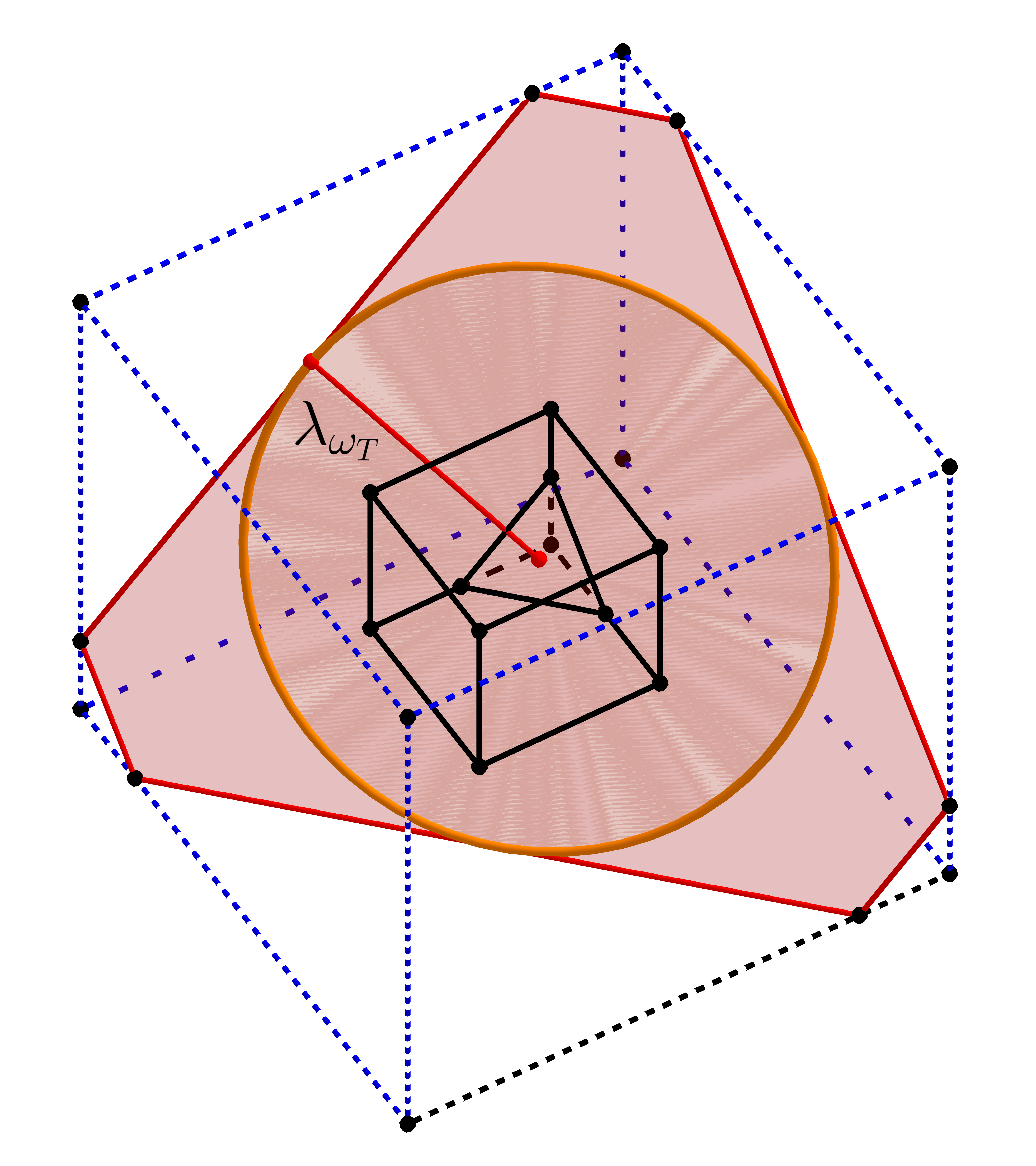

Now, for every interface element , we let be the standard projection operator from to on . Also, since functions in are piecewise polynomials, we can use each of their polynomial components on the whole patch in the following discussion. To analyze the approximation capabilities of local IFE spaces , we consider the following “interpolation” operator on the patch of : such that
| (4.7) |
in which is the extension operator defined in (3.4). By definition, , and our goal is to show that can approximate optimally. The key idea for the analysis of the error in is illustrated by the diagram in Figure 4.2 in which each solid arrow indicates a well-understood relation and our main work is to estimate the difference between and . We will use the following functional to gauge this error:
| (4.8) |
We now show that is a norm equivalent to for functions in .
Lemma 4.4.
is a norm on . Furthermore, there exist constants and such that
| (4.9) |
Proof.
Since is a norm, we only need to prove (4.9). Fix a point , then for each ,
| (4.10) |
where is the Hessian matrix of and it is a constant matrix. Then, we have
| (4.11) |
By Lemma 4.2, we have . Besides, we note that where and are two orthogonal tangential vectors to at . Lemma 4.2 directly implies . Since and can be considered as a two-variable polynomial and its derivatives on , we then apply (4.2), Lemma 4.2 and the inverse inequality given by Lemma 3.3 in [50] to obtain
| (4.12) |
Furthermore, note that is a constant matrix, we have . Putting these estimates into (4.11), we have the first inequality in (4.9). The second inequality in (4.9) directly follows from Lemma 4.1 and the standard inverse inequality for polynomials.
The following lemma is a preparation for the estimation of .
Lemma 4.5.
There exists a constant such that
| (4.13) |
Proof.
Now, we are ready to estimate indicated by the dashed line in the Diagram 4.2.
Lemma 4.6.
Assume that the mesh satisfies the conditions stated in Lemma 4.3. Then there exists a constant such that for every the following holds:
| (4.15) |
Proof.
Let . Since , by Lemma 4.4, we have
| (4.16) |
For the term , using the continuity condition on , i.e., the first equation in (3.3a), the triangular inequality, the trace inequality (4.3), and the estimate (4.6a), we have
| (4.17) | ||||
For the term , firstly, by Lemma 4.5 and the assumption , we have
| (4.18) |
Secondly, using an argument similar to (4.17) with (4.6b) and trace inequality (4.3), we obtain
| (4.19) |
Then, by triangular inequality together with (4.18) and (4.19), we arrive at
| (4.20) |
For the term , using the second condition in (3.3a) and noting that the second derivative of depends only on the coefficient of , we have
| (4.21) |
Finally, putting (4.17), (4.20), and (4.21) into (4.16), we obtain (4.15) for . The results for , , follow from the standard inverse inequality for polynomials.
Then, we have the approximation capabilities of the proposed local IFE space (3.7) on interface elements.
Theorem 4.1.
Assume that the mesh satisfies the conditions stated in Lemma 4.3. Then there exists a constant such that for every the following holds:
| (4.22) |
Proof.
The argument is outlined by the diagram in Figure 4.2. For the case when , we note that . Hence, estimate (4.22) follows directly from the approximation property of the standard projection operator to . For the case when , we note . Thus, (4.22) follows from Lemma 4.6 and the approximation property of the projection operator .
The result in Theorem 4.1 can be also used to analyze the Lagrange type interpolation, i.e., on every interface element , we define such that
| (4.23) |
where are the IFE shape functions determined by (3.16) and , are vertices of . Again, functions in are understood as piecewise functions whose component polynomials can be used on the whole patch . First, we show that the IFE shape functions have bounds similar to those of the finite element shape functions on . We also recall the assumption that .
Theorem 4.2 (Bounds of IFE shape functions).
Let be a mesh satisfying the Assumptions (H1)-(H3). Then, there exists a constant independent of the interface location, mesh size , and coefficients such that
| (4.24) |
Proof.
Since , , we only need to estimate the coefficients and in (3.9). Let be one of the unit vectors in , i.e., , , , , and . Then, under the notations of (3.15) with , the fact and Lemma 3.1 imply
| (4.25) |
where we have used because . Similarly, by (3.15) and , we have
| (4.26) |
where (4.26) is trivial for , since is linear. Putting (4.25) and (4.26) into (3.9), we have (4.24).
Theorem 4.3.
Assume that the mesh satisfies the conditions stated in Lemma 4.3. Then there exists a constant such that for every the following holds:
| (4.27) |
Proof.
Let and , . Note that each can be considered as a function on the whole patch . Using the fact and the triangular inequality, we have
| (4.28) |
Then, by Theorem 4.2, the Sobolev imbedding Theorem and the scaling argument, we have
| (4.29) |
Therefore, (4.27) follows from (4.28) and (4.29) together with the approximation results (4.22).
Since each interface element is a subset of its patch , estimates established in Theorem 4.1 and Theorem 4.3 imply that and can approximate optimally with respect to the underlying polynomials space . As usual, these local optimal approximation capability further imply the optimal approximation capability of the global IFE space defined on the whole . We can see this from the global IFE interpolation operator defined piecewisely such that , in which is given by (4.23) on and the standard Lagrange interpolation on . Then, applying the standard estimation results for the Lagrange interpolation [10] on each non-interface element, summing these estimates and (4.27) over all the elements, and using the finite overlapping property of the patches as well as the extension boundedness (4.1), we have
| (4.30) |
which means that is an optimal approximation of .
5 Numerical Examples
In this section, we present a group of numerical examples to demonstrate features of the proposed IFE space. Since we have known that the proposed IFE space has an optimal approximation capability, we naturally expect that it can be used to solve the interface problem (1.1). For this purpose, we consider the extension of the partially penalized immersed finite element (PPIFE) method [43] for 2-D interface problems to the proposed 3-D IFE space. To describe this method, we use the IFE space defined in (3.19) and consider a bilinear form such that
| (5.1) |
and a linear form such that
| (5.2) |
Then, the PPIFE method for solving the interface problem (1.1) is to find such that
| (5.3) |
where is the subspace of formed by IFE functions with zero trace on , and we tacitly assume that the interface surface does not tough . The terms on interface faces in (5.1) are similar to interior penalties in DG methods [5, 18]; hence, we call this method described by (5.1)-(5.3) symmetric, non-symmetric and incomplete PPIFE (SPPIFE, NPPIFE and IPPIFE) methods when and , respectively.
Numerical results to be reported are generated by applying the PPIFE method to three interface problems posed in the domain whose interface surfaces have three representative geometries as shown in Figures 5.3-5.3, respectively. We only present numerical results of the SPPIFE method because our extensive numerical experiments suggest that the NPPIFE and IPPIFE schemes behave similarly. In particular, we choose the stabilization parameter in (5.1) as , all the data are generated on a sequence of meshes characterized by the mesh size , and the convergence rates are estimated by numerical results on two consecutive meshes.


Spherical Interface: In the first example, the interface problem (1.1) has a simple spherical interface surface as shown in Figure 5.3 defined by a level-set: with and such that and . We choose and in the interface problem (1.1) so that its exact solution is such that on and on with , . The numerical results for the Lagrange interpolation and SPPIFE solutions are presented in Tables 5.1 and 5.2, respectively. These data clearly demonstrate the optimal convergence for both the Lagrange interpolation and SPPIFE solution in and norms. We also note that the convergence rate in norm is close to optimal.
| rate | rate | rate | ||||
|---|---|---|---|---|---|---|
| 1/20 | 1.8969e-03 | 8.6758e-04 | 1.9092e-02 | |||
| 1/30 | 9.3633e-04 | 1.7412 | 4.0365e-04 | 1.8871 | 1.3086e-02 | 0.9316 |
| 1/40 | 5.8322e-04 | 1.6456 | 2.3393e-04 | 1.8963 | 1.0070e-02 | 0.9106 |
| 1/50 | 3.9574e-04 | 1.7379 | 1.5217e-04 | 1.9270 | 8.1492e-03 | 0.9486 |
| 1/60 | 2.7281e-04 | 2.0403 | 1.0675e-04 | 1.9444 | 6.8252e-03 | 0.9724 |
| 1/70 | 2.0707e-04 | 1.7885 | 7.9031e-05 | 1.9504 | 5.8933e-03 | 0.9524 |
| 1/80 | 1.5980e-04 | 1.9407 | 6.0869e-05 | 1.9554 | 5.1697e-03 | 0.9810 |
| 1/90 | 1.2875e-04 | 1.8343 | 4.8356e-05 | 1.9540 | 4.6104e-03 | 0.9722 |
| 1/100 | 1.0540e-04 | 1.8997 | 3.9327e-05 | 1.9616 | 4.1604e-03 | 0.9748 |
| rate | rate | rate | ||||
|---|---|---|---|---|---|---|
| 1/20 | 2.2425e-03 | 1.1204e-03 | 1.9938e-02 | |||
| 1/30 | 1.2337e-03 | 1.4738 | 5.5513e-04 | 1.7319 | 1.3609e-02 | 0.9420 |
| 1/40 | 6.9686e-04 | 1.9855 | 3.0324e-04 | 2.1019 | 1.0328e-02 | 0.9589 |
| 1/50 | 4.4909e-04 | 1.9689 | 1.9187e-04 | 2.0513 | 8.3026e-03 | 0.9781 |
| 1/60 | 3.2664e-04 | 1.7461 | 1.3468e-04 | 1.9411 | 6.9389e-03 | 0.9842 |
| 1/70 | 2.4643e-04 | 1.8280 | 9.7072e-05 | 2.1241 | 5.9748e-03 | 0.9704 |
| 1/80 | 1.8649e-04 | 2.0871 | 7.5467e-05 | 1.8854 | 5.2362e-03 | 0.9883 |
| 1/90 | 1.5431e-04 | 1.6079 | 5.9513e-05 | 2.0165 | 4.6595e-03 | 0.9906 |
| 1/100 | 1.2467e-04 | 2.0243 | 4.8264e-05 | 1.9884 | 4.2026e-03 | 0.9795 |
By the analysis in Section 2 and Section 4, we know that the rules we proposed in Section 2 to form the plane for the construction of IFE functions in each interface element ensure the maximum angle property which further ensure the optimal approximation capability of the IFE space. On the other hand, our extensive numerical experiments indicate that the proposed trilinear IFE space will not possess the expected approximation capability in general if we do not follow these rules to form the plane , and we present two typical groups of data in Tables 5.3 and 5.4 for the corroboration of this observation. In these tables, we employ the following quantities to assess errors in the IFE interpolation of the function described above:
| (5.4) |
Data in Table 5.3 demonstrate the behavior of IFE functions constructed with a “wrong” approximation plane determined by three interface points randomly chosen in each interface element so that the rules proposed for are not always obeyed. The data in this table indicate that these IFE functions do not even show any convergence. In contrast, data in Table 5.4 demonstrate the expected convergence of the IFE functions constructed with formed with the proposed rules. From both the analysis and numerical experiments we can infer that the proposed rules to form the plane for ensuring the maximum angle property is important.
| rate | rate | rate | ||||
|---|---|---|---|---|---|---|
| 1/20 | 1.8665e-03 | 1.1782e-03 | 4.0787e-02 | |||
| 1/30 | 5.0318e-03 | -2.4459 | 1.7692e-03 | -1.0027 | 1.2917e-01 | -2.8431 |
| 1/40 | 1.3626e-03 | 4.5411 | 5.9872e-04 | 3.7663 | 9.4378e-02 | 1.0909 |
| 1/50 | 1.1089e-03 | 0.9231 | 3.7605e-04 | 2.0842 | 5.8381e-02 | 2.1525 |
| 1/60 | 9.6156e-04 | 0.7821 | 3.3370e-04 | 0.6553 | 4.1506e-02 | 1.8712 |
| 1/70 | 2.4471e-04 | 8.8777 | 1.1215e-04 | 7.0737 | 1.6304e-02 | 6.0618 |
| 1/80 | 3.4541e-04 | -2.5812 | 1.3698e-04 | -1.4977 | 3.7622e-02 | -6.2621 |
| 1/90 | 3.9607e-04 | -1.1620 | 1.3758e-04 | -0.0371 | 5.8061e-02 | -3.6840 |
| 1/100 | 2.9810e-03 | 19.1571 | 9.7791e-04 | -18.6146 | 2.2283e-01 | -12.7647 |
| rate | rate | rate | ||||
|---|---|---|---|---|---|---|
| 1/20 | 1.8038e-03 | 1.1782e-03 | 4.0740e-02 | |||
| 1/30 | 9.3633e-04 | 1.6171 | 5.6690e-04 | 1.8043 | 2.8124e-02 | 0.9139 |
| 1/40 | 5.8322e-04 | 1.6456 | 3.2608e-04 | 1.9224 | 2.2490e-02 | 0.7772 |
| 1/50 | 3.7932e-04 | 1.9279 | 2.0603e-04 | 2.0575 | 1.8043e-02 | 0.9874 |
| 1/60 | 2.6949e-04 | 1.8750 | 1.4117e-04 | 2.0736 | 1.4849e-02 | 1.0684 |
| 1/70 | 2.0669e-04 | 1.7211 | 1.0552e-04 | 1.8884 | 1.3165e-02 | 0.7810 |
| 1/80 | 1.5914e-04 | 1.9578 | 8.1105e-05 | 1.9705 | 1.1199e-02 | 1.2115 |
| 1/90 | 1.2674e-04 | 1.9329 | 6.3621e-05 | 2.0615 | 1.0136e-02 | 0.8463 |
| 1/100 | 1.0540e-04 | 1.7502 | 5.2089e-05 | 1.8982 | 9.3055e-03 | 0.8114 |
Orthocircle Interface: In this example, the interface problem (1.1) has an interface surface with a more sophisticated geometry/topology than the one in the previous example. In particular, the interface surface in this example is an orthocircle that is topologically isomorphic to the surface formed by three orthogonal torus as shown in Figure 5.3. The interface can be described by a level-set: with in which
| (5.5a) | ||||
| (5.5b) | ||||
| (5.5c) | ||||
and , . We choose and in the interface problem (1.1) so that its exact solution is , with , . The Lagrange interpolation errors and PPIFE solution errors as well as the related convergence rates are presented in Tables 5.5 and 5.6. The data in these tables clearly demonstrate the optimal convergence, and this example indicates that the proposed IFE method can handle interface problems with quite complicated geometries and topologies.
| rate | rate | rate | ||||
|---|---|---|---|---|---|---|
| 1/30 | 2.0451e-02 | 7.1911e-03 | 1.4047e-01 | |||
| 1/40 | 1.2089e-02 | 1.8274 | 4.0479e-03 | 1.9975 | 1.0539e-01 | 0.9988 |
| 1/50 | 7.9730e-03 | 1.8655 | 2.5916e-03 | 1.9984 | 8.4327e-02 | 0.9993 |
| 1/60 | 5.6492e-03 | 1.8897 | 1.8001e-03 | 1.9989 | 7.0279e-02 | 0.9995 |
| 1/70 | 4.2107e-03 | 1.9066 | 1.3227e-03 | 1.9992 | 6.0243e-02 | 0.9996 |
| 1/80 | 3.2589e-03 | 1.9189 | 1.0128e-03 | 1.9994 | 5.2715e-02 | 0.9997 |
| 1/90 | 2.5967e-03 | 1.9284 | 8.0025e-04 | 1.9995 | 4.6859e-02 | 0.9998 |
| 1/100 | 2.1176e-03 | 1.9358 | 6.4823e-04 | 1.9996 | 4.2174e-02 | 0.9998 |
| rate | rate | rate | ||||
|---|---|---|---|---|---|---|
| 1/30 | 2.0458e-02 | 8.1424e-03 | 1.4051e-01 | |||
| 1/40 | 1.2092e-02 | 1.8278 | 4.6044e-03 | 1.9816 | 1.0552e-01 | 0.9955 |
| 1/50 | 7.9741e-03 | 1.8658 | 2.9566e-03 | 1.9852 | 8.4453e-02 | 0.9979 |
| 1/60 | 5.6498e-03 | 1.8899 | 2.0543e-03 | 1.9969 | 7.0377e-02 | 1.0000 |
| 1/70 | 4.2110e-03 | 1.9067 | 1.5104e-03 | 1.9953 | 6.0326e-02 | 0.9997 |
| 1/80 | 3.2591e-03 | 1.9190 | 1.1575e-03 | 1.9931 | 5.2785e-02 | 1.0001 |
| 1/90 | 2.5969e-03 | 1.9285 | 9.1452e-04 | 2.0001 | 4.6917e-02 | 1.0004 |
| 1/100 | 2.1177e-03 | 1.9359 | 7.4006e-04 | 2.0090 | 4.2220e-02 | 1.0013 |
Interface with Multiple Components: We note that all the results developed in this article can be readily extended to treat interface problems whose interface surface separates the solution domain into more than two subdomains. For a demonstration, the interface surface in this example has multiple components while the interface surfaces in the previous two examples do not have. Specifically, the interface is the union of two disjoint surfaces, one surface is a sphere defined by the level-set where with , , , , the other surface is a torus defined by the level-set where with , . These two interface components separate into three subdomains such that the one inside the torus is , the inside of the sphere is , and . We choose and in the interface problem (1.1) so that its exact solution is on , . The related numerical results reported in Tables 5.5 and 5.6 clearly show the optimal convergence, and this demonstrates that the proposed IFE method can handle the interface problems whose interface consists of disjoint surfaces.
| rate | rate | rate | ||||
|---|---|---|---|---|---|---|
| 1/30 | 5.9738e-02 | 3.2079e-02 | 7.2930e-01 | |||
| 1/40 | 3.6598e-02 | 1.7032 | 1.8643e-02 | 1.8866 | 5.5571e-01 | 0.9450 |
| 1/50 | 2.4701e-02 | 1.7618 | 1.2138e-02 | 1.9231 | 4.4942e-01 | 0.9513 |
| 1/60 | 1.7373e-02 | 1.9301 | 8.5212e-03 | 1.9404 | 3.7737e-01 | 0.9583 |
| 1/70 | 1.2844e-02 | 1.9597 | 6.3182e-03 | 1.9405 | 3.2538e-01 | 0.9617 |
| 1/80 | 1.0528e-02 | 1.4886 | 4.8800e-03 | 1.9343 | 2.8601e-01 | 0.9658 |
| 1/90 | 8.4285e-03 | 1.8886 | 3.8756e-03 | 1.9566 | 2.5511e-01 | 0.9707 |
| 1/100 | 6.8397e-03 | 1.9825 | 3.1525e-03 | 1.9598 | 2.3010e-01 | 0.9794 |
| rate | rate | rate | ||||
|---|---|---|---|---|---|---|
| 1/30 | 8.6433e-02 | 5.4842e-02 | 8.2907e-01 | |||
| 1/40 | 5.0246e-02 | 1.8855 | 2.9779e-02 | 2.1226 | 6.0394e-01 | 1.1013 |
| 1/50 | 3.4425e-02 | 1.6947 | 1.8322e-02 | 2.1766 | 4.7771e-01 | 1.0508 |
| 1/60 | 2.3978e-02 | 1.9836 | 1.2392e-02 | 2.1451 | 3.9665e-01 | 1.0199 |
| 1/70 | 1.7555e-02 | 2.0228 | 8.7675e-03 | 2.2443 | 3.3864e-01 | 1.0257 |
| 1/80 | 1.3198e-02 | 2.1363 | 6.6078e-03 | 2.1179 | 2.9577e-01 | 1.0136 |
| 1/90 | 1.0556e-02 | 1.8961 | 5.1240e-03 | 2.1592 | 2.6214e-01 | 1.0248 |
| 1/100 | 8.6005e-03 | 1.9448 | 4.0734e-03 | 2.1777 | 2.3567e-01 | 1.0102 |
Appendix A Technical Results
In this section, we present the proof of the two technical results.
A.1 Proof of Lemma 3.1
The proof is based on direct calculation. Without loss of generality, we only need to consider the interface element configuration shown in Figure 2.2 with the vertices:
| (A.1) |
and let the subelement containing be . Here, we show a detailed discussion for the Case 1 in Figure 2.2(2(a)). Let , and with , i=1,2,3. Then, we have
| (A.2) |
In addition, note that for this case, then we can verify
| (A.3) |
The results for other cases can be proved by a similar argument, and here, we only list the bounds directly:
- Case 2.
and , .
- Case 3.
and , ,
, . - Case 4.
and , ,
. - Case 5.
and , ,
, .
A.2 Proof of Lemma 4.3
For each , consider a local Cartesian system , , where , span the plane and is perpendicular to . Let be the equation of the surface . Without causing any confusing, we still use to denote points in this local system. For each point , let be the corresponding point on with by (2.9a). Firstly, for (4.6a), we let , then . The Taylor expansion for around yields
| (A.4) |
Then, the triangular inequality yields
| (A.5) |
For the first term in (A.5), we apply the trace inequality (4.3) to obtain
| (A.6) |
For the second term in (A.5), we apply the Hölder’s inequality to obtain
| (A.7) |
For (4.6b), we let , then on where is the normal vector to . Firstly, we use (2.9b) and trace inequality given by Lemma 3.2 in [50] to obtain
| (A.8) |
Note that is in the direction . So by applying the first order Taylor expansion to and using similar argument to (A.5), we have
| (A.9) |
From (A.8), (2.9c) and trace inequality given by Lemma 3.2 in [50], we have
| (A.10) |
Next, by Hölder’s inequality similar to (A.7), we have
| (A.11) |
Finally, substituting (A.10) and (A.11) to (A.9), we arrive at (4.6b).
References
- [1] Slimane Adjerid, Mohamed Ben-Romdhane, and Tao Lin. Higher degree immersed finite element methods for second-order elliptic interface problems. Int. J. Numer. Anal. Model., 11(3):541–566, 2014.
- [2] Slimane Adjerid, Nabil Chaabane, and Tao Lin. An immersed discontinuous finite element method for stokes interface problems. Comput. Methods Appl. Mech. Engrg., 293:170–190, 2015. in press.
- [3] Slimane Adjerid, Nabil Chaabane, Tao Lin, and Pengtao Yue. An immersed discontinuous finite element method for the stokes problem with a moving interface. Journal of Computational and Applied Mathematics, 2018.
- [4] Luca Antiga, Joaquim Peiró, and David A. Steinman. From image data to computational domains, pages 123–175. Springer Milan, Milano, 2009.
- [5] Douglas N. Arnold. An interior penalty finite element method with discontinuous elements. SIAM J. Numer. Anal., 19(4):742–760, 1982.
- [6] Ivo Babuška. The finite element method for elliptic equations with discontinuous coefficients. Computing (Arch. Elektron. Rechnen), 5:207–213, 1970.
- [7] Jinwei Bai, Yong Cao, Xiaoming He, Hongyan Liu, and Xiaofeng Yang. Modeling and an immersed finite element method for an interface wave equation. Computers & Mathematics with Applications, 76(7):1625 – 1638, 2018.
- [8] Charles K. Birdsall and A. Bruce Langdon. Plasma Physics via Computer Simulation (Series in Plasma Physics). Institute of Physisc Publishing, 1991.
- [9] Dietrich Braess. Finite elements. Cambridge University Press, Cambridge, second edition, 2001. Theory, fast solvers, and applications in solid mechanics, Translated from the 1992 German edition by Larry L. Schumaker.
- [10] Susanne C. Brenner and L. Ridgway Scott. The mathematical theory of finite element methods, volume 15 of Texts in Applied Mathematics. Springer, New York, third edition, 2008.
- [11] Erik Burman, Susanne Claus, Peter Hansbo, Mats G. Larson, and André Massing. Cutfem: Discretizing geometry and partial differential equations. International Journal for Numerical Methods in Engineering, 104(7):472–501, 2015.
- [12] Long Chen, Huayi Wei, and Min Wen. An interface-fitted mesh generator and virtual element methods for elliptic interface problems. Journal of Computational Physics, 334(1):327–348, 2017.
- [13] Zhiming Chen and Jun Zou. Finite element methods and their convergence for elliptic and parabolic interface problems. Numer. Math., 79(2):175–202, 1998.
- [14] C.-C. Chu, I. G. Graham, and T.-Y. Hou. A new multiscale finite element method for high-contrast elliptic interface problems. Math. Comp., 79(272):1915–1955, 2010.
- [15] Ray. W. Clough and James L. Tocher. Finite element stiffness matrices for analysis of plate bending. In Matrix Methods in Structual Mechanics, pages 515–545, 1966.
- [16] F. Dassi, S. Perotto, L. Formaggia, and P. Ruffo. Efficient geometric reconstruction of complex geological structures. Mathematics and Computers in Simulation, 106:163 – 184, 2014. Applied Scientific Computing X: Advanced Meshing and Simulations Approaches - Edited by: Angel Plaza and Rosa Maria Spitaleri and Applied Scientific Computing XI: Effective Numerical approaches for complex problems - Edited by Rosa Maria Spitaleri.
- [17] John Dolbow, Nicolas Moës, and Ted Belytschko. An extended finite element method for modeling crack growth with frictional contact. Comput. Methods Appl. Mech. Engrg., 190(51-52):6825–6846, 2001.
- [18] Jim Douglas, Jr. and Todd Dupont. Interior penalty procedures for elliptic and parabolic Galerkin methods. In Computing methods in applied sciences (Second Internat. Sympos., Versailles, 1975), pages 207–216. Lecture Notes in Phys., Vol. 58. Springer, Berlin, 1976.
- [19] Yalchin Efendiev and Thomas Y. Hou. Multiscale finite element methods, volume 4 of Surveys and Tutorials in the Applied Mathematical Sciences. Springer, New York, 2009. Theory and applications.
- [20] H. Federer. Curvature measures. Trans. Amer. Math. Soc., 93:418–491, 1959.
- [21] F. Fogolari, A. Brigo, and H. Molinari. The poisson–boltzmann equation for biomolecular electrostatics: a tool for structural biology. Journal of Molecular Recognition, 15(6):377–392, 2002.
- [22] Ruchi Guo. Design, Analysis, and Application of Immersed Finite Element Methods. PhD thesis, Virginia Polytechnic Institute and State University, 2019.
- [23] Ruchi Guo and Tao Lin. A group of immersed finite element spaces for elliptic interface problems. IMA J.Numer. Anal., page drx074, 2017.
- [24] Ruchi Guo and Tao Lin. A higher degree immersed finite element method based on a cauchy extension. SIAM J. Numer. Anal. (accepted), 2019.
- [25] Ruchi Guo, Tao Lin, and Yanping Lin. Approximation capabilities of immersed finite element spaces for elasticity interface problems. Numer. Methods Partial Differential Equations, 35(3):1243–1268, 2018.
- [26] Ruchi Guo, Tao Lin, and Yanping Lin. A fixed mesh method with immersed finite elements for solving interface inverse problems. J. Sci. Comput. (in press), 2018.
- [27] Ruchi Guo, Tao Lin, and Xu Zhang. Nonconforming immersed finite element spaces for elliptic interface problems. Comput. Math. Appl., 75(6):2002 – 2016, 2018.
- [28] Ruchi Guo, Tao Lin, and Qiao Zhuang. Improved error estimation for the partially penalized immersed finite element methods for elliptic interface problems. Int. J. Numer. Anal. Model., 16(4):575–589, 2018.
- [29] Johnny Guzmán, Manuel A. Sánchez, and Marcus Sarkis. Higher-order finite element methods for elliptic problems with interfaces. ESAIM: Mathematical Modelling and Numerical Analysis, 50(5):1561–1583, 2016.
- [30] Johnny Guzmán, Manuel A. Sánchez, and Marcus Sarkis. A finite element method for high-contrast interface problems with error estimates independent of contrast. Journal of Scientific Computing, 73(1):330–365, 2017.
- [31] Anita Hansbo and Peter Hansbo. An unfitted finite element method, based on Nitsche’s method, for elliptic interface problems. Comput. Methods Appl. Mech. Engrg., 191(47-48):5537–5552, 2002.
- [32] Xiaoming He, Tao Lin, and Yanping Lin. Approximation capability of a bilinear immersed finite element space. Numer. Methods Partial Differential Equations, 24(5):1265–1300, 2008.
- [33] Xiaoming He, Tao Lin, Yanping Lin, and Xu Zhang. Immersed finite element methods for parabolic equations with moving interface. Numer. Methods Partial Differential Equations, 29(2):619–646, 2013.
- [34] R. W. Hockney and J. W. Eastwood. ComputerSimulationUsingParticles. Taylor & Francis, Inc., Bristol, PA, USA, 1988.
- [35] David Holder and Institute of Physics (Great Britain). Electrical impedance tomography: methods, history, and applications. Institute of Physics Pub, 2005.
- [36] R. Kafafy, T. Lin, Y. Lin, and J. Wang. Three-dimensional immersed finite element methods for electric field simulation in composite materials. Internat. J. Numer. Methods Engrg., 64(7):940–972, 2005.
- [37] Randall J. LeVeque and Zhi Lin Li. The immersed interface method for elliptic equations with discontinuous coefficients and singular sources. SIAM J. Numer. Anal., 31(4):1019–1044, 1994.
- [38] Randall J. LeVeque and Zhilin Li. Immersed interface methods for Stokes flow with elastic boundaries or surface tension. SIAM J. Sci. Comput., 18(3):709–735, 1997.
- [39] Z. Li, T. Lin, Y. Lin, and R. C. Rogers. An immersed finite element space and its approximation capability. Numer. Methods Partial Differential Equations, 20(3):338–367, 2004.
- [40] Zhilin Li and Kazufumi Ito. The immersed interface method, volume 33 of Frontiers in Applied Mathematics. Society for Industrial and Applied Mathematics (SIAM), Philadelphia, PA, 2006. Numerical solutions of PDEs involving interfaces and irregular domains.
- [41] Zhilin Li and Ming-Chih Lai. The immersed interface method for the Navier-Stokes equations with singular forces. J. Comput. Phys., 171(2):822–842, 2001.
- [42] Tao Lin, Yanping Lin, and Xu Zhang. A method of lines based on immersed finite elements for parabolic moving interface problems. Adv. Appl. Math. Mech., 5(4):548–568, 2013.
- [43] Tao Lin, Yanping Lin, and Xu Zhang. Partially penalized immersed finite element methods for elliptic interface problems. SIAM J. Numer. Anal., 53(2):1121–1144, 2015.
- [44] Tao Lin, Qing Yang, and Xu Zhang. A Priori error estimates for some discontinuous Galerkin immersed finite element methods. J. Sci. Comput., 2015. in press.
- [45] J. M. Melenk and I. Babuška. The partition of unity finite element method: basic theory and applications. Comput. Methods Appl. Mech. Engrg., 139(1-4):289–314, 1996.
- [46] J.M. Morvan and B. Thibert. On the approximation of a smooth surface with a triangulated mesh. Computational Geometry, 23(3):337 – 352, 2002.
- [47] N. Sukumar, D. L. Chopp, N. Moës, and T. Belytschko. Modeling holes and inclusions by level sets in the extended finite-element method. Comput. Methods Appl. Mech. Engrg., 190(46-47):6183–6200, 2001.
- [48] N. Sukumar, Z. Y. Huang, J. H. Prévost, and Z. Suo. Partition of unity enrichment for bimaterial interface cracks. Internat. J. Numer. Methods Engrg, 59(8):1075–1102, 2004.
- [49] Sylvain Vallaghé and Théodore Papadopoulo. A trilinear immersed finite element method for solving the electroencephalography forward problem. SIAM J. Sci. Comput., 32(4):2379–2394, 2010.
- [50] Fei Wang, Yuanming Xiao, and Jinchao Xu. High-order extended finite element methods for solving interface problems. arXiv:1604.06171v1, 2016.
- [51] Joseph Wang, Xiaoming He, and Yong Cao. Modeling Electrostatic Levitation of Dust Particles on Lunar Surface. IEEE Transactions on Plasma Sciences, 36(5):2459–2466, 2008.
- [52] T. Warburton and J. S. Hesthaven. On the constants in -finite element trace inverse inequalities. Comput. Methods Appl. Mech. Engrg., 192(25):2765–2773, 2003.
- [53] Dexuan Xie and Jinyong Ying. A new box iterative method for a class of nonlinear interface problems with application in solving poisson–boltzmann equation. Journal of Computational and Applied Mathematics, 307:319 – 334, 2016. 1st Annual Meeting of SIAM Central States Section, April 11–12, 2015.
- [54] Jinchao Xu. Estimate of the convergence rate of the finite element solutions to elliptic equation of second order with discontinuous coefficients. Natural Science Journal of Xiangtan University, 1:1–5, 1982.
- [55] Xu Zhang. Nonconforming Immersed Finite Element Methods for Interface Problems. PhD thesis, Virginia Polytechnic Institute and State University, 2013.