Computing genera of satellite tunnel number one knots and torti-rational knots
Abstract.
The genus of satellite tunnel number one knots and torti-rational knots is computed using the tools introduced by Floyd and Hatcher [4]. An implementation of an algorithm is given to compute genus and slopes of minimal genus Seifert surfaces for such knots.
Key words and phrases:
rational 2-bridge links, genus, spanning surfaces, satellite tunnel number one knots, torti-rational knots.1991 Mathematics Subject Classification
57M251. Introduction
A family of knots widely studied is the one known as -knots, these are knots which can be put in 1-bridge position with respect a standard torus in . This family contains all 2-bridge knots, all satellite tunnel number one knots, and it is contained in the family of tunnel number one knots. Genus one and genus two -knots have been classified in [9] and [3], respectively. It is natural to ask for a classification of -knots of any genus . Such knots are divided into the satellite and the non-satellite cases. For the non-satellite case we expect to have a description similar to that in [3], as special banding of two -knots of smaller genus. In the case that the knot is satellite, we need to determine the 4-tuple of the Morimoto-Sakuma construction that produces satellite genus tunnel number one knots [11]. The parameters describe a rational link and a companion torus knot. For genus a minimal Seifert surface may intersect the companion torus in a non-empty collection of longitudes, hence the surface is broken into two pieces, one piece consists of Seifert surfaces for the companion torus, the other piece is a surface contained in the neighborhood of the torus knot with one boundary parallel to the satellite knot and boundary components which are slopes on the companion torus. Such a surface defines an essential surface for the link , with one boundary parallel to a component of the link and a number of boundary components on the other component. Floyd and Hatcher [4] classified essential surfaces for rational links. Later Hoste and Shanahan [8] classified the slopes of such surfaces. However the calculation of genera of the surfaces is not given there.
We were able to determine that an essential surface for a rational link with one boundary on one component of the link and a number of boundary slopes on the other component of the link, arises from at most two minimal edge-paths of the Floyd-Hatcher construction, by means of continued fraction expansions for . This gives a constructive description of the surfaces and allows to compute genus and slope of the surface, as well as to determine whether or not the surface is a fiber of a fibering over the circle for the link.
Applying these results to satellite tunnel number one knots we obtain the following result:
Theorem 1.
Let be the 2-bridge link given by the tunnel number one satellite knot . Suppose . Then
- (1)
If , and is the unique continued fraction for with odd, the genus of is:
where
- (2)
If , and is the unique continued fraction for with odd, the genus of is:
where
Corollary 2.
Let be a tunnel number one satellite knot such that . Then the genus of is:
It is worth mentioning that Hirasawa and Murasugi [7] obtained similar results using the Alexander polynomial.
We can also apply our technique to compute the genus of torti-rational knots, which are obtained from a rational link by performing -Dehn twists along one component of the link.
Theorem 3.
Let be a torti-rational knot and a minimal genus Seifert surface for it. Suppose that . Then:
- (1)
If and is the unique continued fraction for with odd, the genus of is:
where
- (2)
If and is the unique continued fraction for with odd, the genus of is:
where
- (3)
If and . Let be the continued fraction expansion for with or such that and for all . The genus of is:
- (4)
If and and and are the continued fraction for with odd. The genus of is:
For the case that for both cases we prove:
Theorem 4.
When the linking number is zero, the genus of a satellite tunnel number one knot is one half the wrapping number of in . Moreover, if is the continued fraction expansion for with or such that odd, the genus of is . The same is true for a torti-rational knot.
Theorems 1 and 3 required a decomposition of as a continued fraction and some computations. We have written an algorithm that receives as inputs and outputs genus, slopes and number of boundary components for the surface, at some cases it can determined the fiberedness of the knot.
Our algorithm is based on that given by Hoste and Shanahan. We found a fault for rationals , thus it was necessary to reprogram this algorithm to compute the paths and to incorporate computations of genus, slopes and number of boundary components. Our modification of their algorithm can be found at https://github.com/viorato/compute_rational_links_genus.
In Section 2 we review the concepts from Floyd-Hatcher which are necessary to develop our techniques. In Section 3 we state the basic results that allow to describe the specific type of edge-paths associated to the surfaces of our interest. Using continued fraction expansions for we compute genus and slopes for the surfaces in Section 3.1. We revisite Floyd-Hatcher to give their criteria for a surface to be a fiber of a fibering for a rational link and give a criteria in terms of the continued fraction expansions for our surfaces to be fibers in Section 4. Finally in Section 5 we compute the genus for satellite tunnel one knots and for torti-rational knots.
2. Preliminaries
2.1. The diagram of slope system in the four puncture sphere
A 2-bridge link is represented by a rational number . We may suppose , even, and . We say that a surface in is essential if it is incompressible, -incompressible and not boundary parallel. The main idea of Floyd and Hatcher’s [4] construction is to associate to an essential surface in an edge-path from to in the Diagram , , shown in Figure 1.
The diagram is an embedded graph on the upper half plane with the real line and the point at infinite . Its vertices are the rational points in , and its edges are hyperbolic lines in the upper half model of joining two vertices , , if and only if . These lines are the edges of ideal triangles in , and is the group of orientation-preserving symmetries of this ideal triangulation. The diagram is transformed onto the Poincaré disk model by , see Fig.1. Let be the subgroup of Möbius transformations with even. Its fundamental domain is the triangle . Consider the ideal quadrilateral . The -images of this quadrilateral tessellate . We form the diagram from by deleting the -orbit of the diagonal of and adding the -orbit of the opposite diagonal . The diagram , , , is obtained from by deleting the diagonal in each quadrilateral , and adding a small rectangle having a vertex in the interior of each edge of so that for . The edges of fall into four -orbits, labelled , , , .


Remark 5.
As approaches to 0 and 1, the inscribed rectangle collapses to the diagonals or to the diagonal , respectively. See Figure 2.

For a given reduced rational number , let denote an oriented edge-path from to in with .
Definition 6.
An edge-path is called minimal if no two consecutive edges in lie on the boundary of the same triangle face or rectangle face in .
Then for every minimal edge-path in , Floyd-Hatcher construct a corresponding branched surface . Four basic branched surfaces, , , , and are assigned to the labelled edges. See figure 3.

We regard as the two point compactification of and we place the link so that it meets and each in two arcs and each intermediate level in four points. We think of each level as the quotient , where is the group generated by rotations of about the integer lattice points . The four points of the link at each intermediate level are precisely the four points of . The two arcs at level have slope and those arcs at level have slope . acts linearly on the level sphere , leaving invariant.
The vertices of the diagrams correspond to the slopes of arcs in the level spheres.
Let be the sequence of edges of a minimal edge-path . An edge is the image of one of the four edges, , , , , see Figure 1(c), under a unique . To get we first apply to the appropriated surface , , , or , and then scale vertically into interval .
Finally, a surface carried by one of the branched surfaces is determined by and , the numbers of sheets of the surface along each component of the 2-bridge link , and by how the surface branches in each segment , , , or of . We set , which is the subscript of .
Floyd and Hatcher proved that every essential surface in is carried by some branched surface corresponding to a minimal edge-path from to in , and, conversely, an orientable surface carried by such a branched surface is essential.
A branched surface may carry non-orientable surfaces. Moreover, there may be an essential non-orientable surface which is not carried by any branched surface.
There is a unique finite sequence of quadrilaterals such that the first one contains the vertex , the last one contains the vertex and every pair of consecutive ones intersects in a single edge.
Remark 7.
In a diagram with , the first and the last edges in any edge-path are of type .
2.2. Edge-paths and essential saddles
Let be a compact orientable essential surface with boundary on .
We may isotope so that:
- (1)
Each component of is either a meridian of in , or is transverse to all meridians of .
- (2)
is transverse to and lies in near .
- (3)
The projection is a Morse function with all its critical points in the interior of .
A transverse intersection , , for , can contain no arcs which are peripheral in , in view of and the -incompressibility of . As varies from 0 to 1, the point can change only at critical levels of the projection , in fact, only at saddles. A saddle where changes we call an essential saddle. So we obtain a finite sequence of s, say , with for all . By , is the vertex of and is the vertex .
We can isotope to lie in and have all its critical points essential saddles, and also still satisfy above, see section 7 of [4].
The possibilities, up to level-preserving isotopy, for an essential saddle corresponding to a segment on an or type edge of are shown in Figure 4. The two leftmost vertices depict and the rightmost vertices depict .


The corresponding saddle to an or type edge of , will be called an or type saddle, respectively.
3. General results
Let be a rational link embedded in and let be a connected, compact, essential and orientable surface, both as in Section 2.2. Assume that has -boundary components in , which are non-meridional and , i.e, is a multiple of ; and has one boundary component parallel to , i.e, . Let us denote by the set of boundary components of , for . Observe that consists only of one curve whose slope is an integer; and of parallel curves with slope , with respect a meridian and preferred longitude in each component of the link. We denote the linking number of by .
In the following lemmas we will determine the saddle types corresponding to a minimal edge-path associated to . Since there is a bijective correspondence between edges, saddles and pieces of branched surfaces, the results can be applied to the three concepts.
Since and by Remark 7 the first and last saddles are of type . By Lemma 7.1 and Figure 7.2 of [4], we have the following statement:
Lemma 8.
Suppose that .
- (1)
type saddles come in groups of saddles.
- (2)
type saddles come in groups of saddles.
Next we will prove that only edges of type and can occur. Choosing an orientation for will induce an orientation on the boundary components of and on the arcs of , for before the first type saddle; choose one. When two arcs are being fused by a saddle, in a small neighborhood before the fusion occurs, we see two small arcs with opposite orientations.
Lemma 9.
There are no -type saddles.
Proof.
At the first level, , there is only one arc of connecting the vertices of . This implies that, in a small neighborhood around one of the vertices of , we see only one arc pointing out and around the other vertex we see only one arc pointing in; we see opposite orientations around these vertices. This property must be preserved for all the different levels .
Now, if a -type saddle exists then, after a transformation, it looks like in Fig. 4(c) . But that will imply that the orientations around the vertices , at some , are no longer opposite.
∎
One crucial object that we used on the proof of Lemma 9 and that we will use is the orientation of around a small neighborhood of a vertex. Once that we orientate , it induces an orientation on the arcs around a vertex, we can assign a to each arc pointing out and a to an arc pointing in. We can then compute the sum of the signs around a vertex ; we denote it as . Observe that is independent of the level and it reverses its sign if we change the orientation of . So, is a constant that is independent of the level and the orientation of .
Lemma 10.
If the boundary slope of is of the form with . Then for each vertex in
Proof.
By definition, we can compute around any meridian of . And this can be done by computing the intersections with signs of and . As the slope of is , each boundary component of intersects exactly times, let be the number of the components intersecting positively and the number of components which intersect negatively, then .
Now, we only need to prove that . This can easily be seen by observing that represents an equivalence between and on and later combine it with the relations and .
∎
From the previous proof, it seems that we could get rid of the absolute values from the statement. But the problem is that our definition of has an ambiguity on its sign, it is possible to avoid it by being more specific on its definition, but we wouldn’t win much; it is more convenient to use and compute .
Lemma 11.
Suppose that , and let be a surface given by an edge-path in .
- (1)
If there is a type saddle, then for all in . Moreover, each boundary component of in is longitudinal and .
- (2)
If there is a type saddle, then for all in . Moreover, all boundary components of have the same orientation.
Proof.
(1) By Lemma 8 the number of arcs in joining the components of is odd. Before a type saddle appears, there must be an type saddle. After passing it, we see an even number of arcs joining the components of . In order to perform a type saddle, two arcs of the same slope must be joined; thus their orientation are opposite. So, all the arcs joining the components of can be paired together on opposite orientation pairs. This implies that for each vertex .
By Lemma 10, we have that the slope is equal to , hence is an integer (its components are longitudinal).
(2) After a transformation, a type saddle looks like in Fig. 4(d). When performing a type saddle, the configuration of arcs that we obtain contains two arcs of slope zero whose orientations coincide with the one on the previous arcs of slope zero. This occurs every time we perform a type saddle, and by Lemma 8 this happens times, thus the arcs joining the components of have the same orientation. So, .
∎
Corollary 12.
If there is a type saddle and if the boundary slope of equals then and
Summarizing we have:
Corollary 13.
Let be a rational link embedded in and let be a connected, compact, essential and orientable surface. Assume that has -boundary components in , which are non-meridional and , i.e, is a multiple of ; and has one boundary component parallel to , i.e, . Then the sequence of saddles consists only of and type saddles; or only of and type saddles; otherwise we will have but .
Definition 14.
We will use the notation edge-path to refer to an edge-path consisting of only and type saddles. Similarly we use the notation - and edge-path.
When the sequence of saddles is an edge-path. In this case , thus the corresponding edge-path lies in the diagram and there are no types saddles by Lemma 9.
If is oriented surface with then it comes from an edge-path. Nevertheless, not all edge-path correspond to an orientable surface.
For instance, consider the edge-path , , , , the corresponding sequence of saddles is , see Figure 5. In Figure 6 we shown the first part of the saddle sequence (recall that we are using type saddle). Observe that passing to the third saddle of type gives rise a nonorientable surface.

The same observation is valid for or edges-paths; namely, there are such edge-paths that correspond to non-orientable surfaces. The next Lemma rules out edge-paths corresponding to non-orientable surfaces. In order to state the result, we introduce some notation.
Each reduced fraction in can be identified with , or by reducing and mod 2. An type edge in is contained in an edge . If is identified with mod 2, we say that such and edge is of type . On the other hand if is identified with the edge is said to be of type .
By an edge-path we will mean an edge-path in that consists only of edges of type and with and . Similarly we use the notation edge-path for an edge-path in that contains only type edges with .
Lemma 15.
Let be an orientable surface and be an edge-path in associated to . Suppose that is an edge-path with . Then is an -edge-path with . The same result is valid for edge-paths.
Proof.
Assume that contains edges of type and . We are going to find a contradiction.
Case 1: is an -edge-path in . As is made of only type saddles, there must be two consecutive saddles of type and . Without loss of generality, we can assume that follows . We draw the sequence of pictures module 2 for these two saddles in Fig. 7. Notice that this is impossible due to orientability of .
Case 2: is an -edge-path in . Again, in this case we will have two consecutive saddles of type and ; because the edge-path comes in blocks of the form where the two are of the same type. The sequence of levels mod 2 is similar to the previous one, see Fig. 8, but with some extra parallel arcs.
By Lemma 11a those parallel arcs must have all the same orientation; moreover, around the vertices in , all the arcs are oriented in the same direction. Is not hard to see from Fig. 8 that it is impossible to give a coherent orientation to all the arcs with the condition that all the parallel arcs have the same orientation, contradicting the orientability of .
Case 3: is an -edge-path in . A similar phenomenon to the previous case happens here. In fact, we get the same picture as in Fig. 8. The reason is that the edge-paths come in blocks of the form where the two ’s are of the same type. So, if we have two ’s of a different type on , there must be two consecutive blocks with different -types.
As consequence of lemma 11b, all the arcs in the first and last level in Fig. 8 need to be cancel in pairs. And again it becomes impossible to give a coherent orientation satisfying these conditions.
∎
Remark 16.
When an edge-path happens it must be of the form , where the and type edges lie in different polygons, see Fig. 1(c). Since the surfaces considered in this work are connected, an edge-path consists of at least two blocks.
Remark 17.
In the case that has meridional boundary components in and one boundary component parallel in , then the edge-path corresponding to the branched surface that carries belong to the diagram . Thus it is an edge-path. For type edges to exist and to obtain an orientable surface it must happen that greater than . See Figures 9(a) and 9(b) of and type saddle for . We conclude that in this case, the edge-path consists only of type edges.


3.1. Continued fractions and genus of surfaces
We recall from Hatcher and Thurston [6]: an edge-path from to in the diagram corresponds uniquely to a continued fraction expansion , where the partial sums are the successive vertices of the edge-path.
Remark 18.
At the vertex the path turns left or right across triangles. For odd, right if and left if . For even left if and right if . The number of diagonals is
By Remark 5, in the diagonals of the diagram are changed by inscribed rectangles. So for each diagonal we obtain a edge around the vertex , see Fig 1(a). Thus the number of edges around is .
In this paper we use two special types of continued fraction expansions: and . These are the unique continued fraction where each entry is an even number and are odd.
We will described the edge-path in associated to these continued fractions, such that the branched surface associated carries a connected, compact, essential and orientable surface with one boundary component parallel to and -boundary components in , which are non-meridional and ; i.e, and is a multiple of . For now on we assume that .
For short we will say that the surface is associated to the edge-path. We will compute the genus of as well.
For both continued fraction expansions, the vertices , given by the partial sums, satisfy that is even and is odd.
In the diagram , the edge-path for passes by ; and the edge-path for passes by . These are edge-paths.
The edge-path corresponding to the continued fraction is an edge-path, and the corresponding to the continued fraction is a edge-path.
If , then the edge-path just obtained; is the one that corresponds to . Hence we obtain an edge-path of length ( or ), where each edge lies in different triangles by construction. For each type edge we have an type saddle, thus we can compute the genus of using Euler characteristic.
Proposition 19.
Let be one of two the continued fractions expansions for . If , the associated edge-path consisting of edges; corresponds to a connected, compact, essential and orientable surface with one boundary component parallel to for . Then the genus of is
∎
If , we pass to the diagram with . Each edge in is changed into an edge and a edge. The edge path in is transformed into an -edge-path in a diagram . Around a vertex with even denominator there are only type edges, and around a vertex with odd denominator there are only type edges. Thus the pattern is repeated -times (or -times).
Observe that an edge-path obtained as above may not correspond to a minimal edge-path in ; nevertheless a minimal edge-path associated to a connected, compact, essential and orientable surface is in correspondence with an edge-path with . A condition on the continued fraction expansion for for an edge-path to be minimal is that greater than 1 for all .
If an orientable surface is carried by this kind of path, Lemma 11 implies and by Remark 16 we have (or ; since we require a connected surface, where are the lengths of the continued fraction expansions for . Hence an -edge-path that passes trough the vertices or associated to an orientable surfaces must contained at least two blocks of the pattern , thus the continued fraction expansion must contain at least three even terms, after the 0 or 1 entries.
In order to compute the genus of , the associated surface to this edge-path, we count the number of saddles corresponding to the edge-path. Observe that each type edge corresponds to one saddle and each type edge to -saddles. Each block of contributes with saddles. Again, using Euler characteristic we find:
Proposition 20.
Let be one of two the continued fractions expansions for , with and for all . If and the associated -edge-path; consisting of blocks; corresponds to a connected, compact, essential and orientable surface with one boundary component parallel to and -boundary components parallel to . Then the genus of is:
∎
If is oriented and then the edge-path for is an -edge-path. In this case, we substitute each pair in the above edge-path by a sequence , where the number of ’s is given by the number of diagonals in the diagram around the corresponding vertex. For instance, if , the number of ’s is .
Summarizing, the edge-type in associated to the continued fraction expansion is
. Notice that the two consecutive type edges belong to different triangles, and the type edges belong to different quadrilaterals by construction. Thus we obtain a minimal edge-path.
Analogously, for the continued fraction expansion we associate an edge-path.
Next we compute the genus of such .
Proposition 21.
Let be one of two the continued fractions expansions for . If and the associated path corresponds to a connected, compact, essential and orientable surface with one boundary component parallel to and -boundary components non-meridional on . Then the genus of is:
where
Proof.
Use Euler characteristic, considering that each type edge corresponds to one saddle and each type edge corresponds to saddles. ∎
3.2. Boundary slopes
The boundary of a branched surface derived from the Hatcher-Floyd construction defines a train track on the boundary of the regular neighborhood of the link. Thus the boundary of any essential surface carried by the branched surface is carried by this train track. Lash, [10], calculated the space of boundary slopes for the Whitehead link.
In the following paragraph we explain Lash algorithm. We base the explanation on the article [5]:
To compute the boundary slopes of the surfaces the frame used consists of the meridian and a non-standard longitude of . In , we take the arc of slope connecting and . is the union of the arc and an arc in . is oriented toward increasing along the axis . The meridian is oriented as a right-handed circle around the axis oriented upward. We obtain from by rotating by about the axis .
Let be the algebraic intersection number in . Let be the map such that for , . For , , contributes to the number as in Table 1, if the orientations of and agree. If they disagree, we change all the sign of the number in Table 1.
We calculate the boundary slope of a surface corresponding to an -edge-path.
Taking the sum of the entries of the row of and of Table 1, we can see that the slope on is and that on is , where the first coordinate is the longitudinal entry, and the second coordinate is the meridional entry with respect to the unusual longitude . To obtain the real slope, we need to know the slope of the preferred longitude, which is obtained by substituting for and for , in , which is . The preferred longitude of is of slope , which is obtained by substituting and in . But the preferred longitude of is the same for , recall that we take as the image of by rotating about the axis . Thus, and . The slopes with respect to the preferred longitude can be obtained from on , and on .
| Label | condition on | ||
|---|---|---|---|
| A | |||
| B | 0 | ||
| 0 | |||
| C | 0 | ||
| otherwise | |||
| D | |||
| otherwise |
Recall that we are considering two types of continued fraction expansions for , namely and . As discussed in Section 3.1, for each continued fraction there is an -edge-path corresponding to an essential surface. We will determined the contribution of .
The edge path for is , the orientations of the edges and need to be determined in order to compute . If the orientation of and with agree we denote the edge by , if they disagree we denote it by .
By the construction of the edge path is not hard to see that, see Figure 10:
- (1)
The first type edge is an .
- (2)
The first type edges are .
- (3)
Each intermediate pair is of the form .
- (4)
The last type edge is
For the remaining type edges we have:
Proposition 22.
For the continued fraction expansion and odd.
- (1)
If then the sequence of type edges are .
- (2)
If then the sequence of type edges are .
Proof.
For both cases we need to verify that the agreement or disagreement of the types edges with at the th position for odd. Since we are considering the continued fraction , all the vertices , for -odd, are congruent with mod 2, up to transformations of elements of . Thus the type edge at such vertex is a edge. See Figure 10. From Remark 18 the quadrilateral turns right if and left if . Hence, if the sequence of type edges are and if the sequence of type edges are . See Figures 10 and 11 for the turns around mod 2. ∎

The value of for the edge path corresponding to the continued fraction expansion is because when we see type edges, so the contribution in the Table 1 is , and if we see type edges, so they contribute with in Table 1. Since , we conclude the following:
Corollary 23.
Let be a surface associated to the edge path
, arising from .
The boundary slopes of with respect to the preferred longitude on is and on is .
On the other hand; for the continued fraction expansion the corresponding edge path in the diagram is . This path lies in the same sequence of quadrilaterals as the corresponding path for the continued fraction expansion , but it is made of the and type edges which do not belong to the path for . Reasoning as before, we have that for the edge-path corresponding to :
- (1)
The first type edge is an .
- (2)
The first type edges are .
- (3)
Each intermediate pair is of the form .
- (4)
The last type edge is
Proposition 24.
For the continued fraction expansion and odd.
- (1)
If then the sequence of type edges are .
- (2)
If then the sequence of type edges are .
Corollary 25.
Let be a surface associated to the edge path
, arising from .
The boundary slopes of with respect to the preferred longitude on is and on is .
Analogously, we can compute the boundary slopes for -edge-path and -edge-path, in both cases the resulting boundary slopes are equal to zero.
4. Fiberings
Floyd and Hatcher give a criterion to determine when a surface in is a fiber of a fibering .
Definition 26.
Let be a path in , with . A maximal sequence of consecutive and type edges in each separated from the next by only one edge in , is called a string.
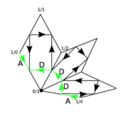

Proposition 6.1 of [4] states sufficient and necessary conditions for fibering:
Proposition 27.
A surface in is a fiber of a fibering if and only if it is isotopic to a surface carried by a branched surface whose associated edge-path from to , in a determined , consists of a single string of and type edges.
The following theorem tells us conditions on the continued fraction expansion, considered in this work, for a surface to correspond to a fiber of a fibering .
Theorem 28.
Let be a link and a surface in .
- (1)
Suppose is associated to an -edge-path. is a fiber of a fibering if and only if the continued fraction expansion for has the form with and .
- (2)
Suppose is associated to an -edge-path. is a fiber of a fibering if and only if the continued fraction expansion for has the form with and for all .
- (3)
Suppose is associated to a -edge-path. is a fiber of a fibering if and only if the continued fraction expansion for has the form with positive for all . Thus the fraction starting with 1, is of the form with negative for all .
Proof.
In each case we need to verify that the corresponding path in the adequate diagram is a string.
- (1)
Let be the edge-path arising from the continued fraction expansions . Observe that any two consecutive and are separated by exactly one type edge in , with . And any two consecutive type edges are separated by exactly one or type edge, see Figures 12(a) and 12(b). To guarantee that is a single string, it is necessary to check when two consecutive type edges are separated by only one edge. By inspecting Figure 12(b), is easy to observe that two type edges are separated by only one edge if . This pattern is extended to the whole path . Thus the condition is that with for -even in the continued fraction expansion .
- (2)
Consider the continued fraction expansion , since is associated an -edge-path in diagram, goes through all the vertices . For to be a string, every two consecutive -type edges must be separated by exactly one -type edge or by exactly on -type edge. There are two possibilities depicted in Figures 13(a) and 13(b), we see that for all . Thus the continued fraction expansion has the form with .
- (3)
Let us consider the continued fraction expansion , in this case the surface is in correspondence with a -edge-path in the diagram. The first edges of type pass through vertices . Each two consecutive -type edges are separated by exactly one -type edge. Thus, that piece of satisfies the condition to be a string. See Figure 14(a). A similar phenomenon occurs around a vertex with -even. It is necessary to determine when two consecutive -edges with common vertex with -odd are separated by exactly one -edge.
Next we will determine conditions for in order to keep being a string, up to transformation, we will be able to argue that the conditions for can be extended to the following .
First let us consider both positive. The -edge connecting and has to turn left -edges to reach the vertex . Then the edge connecting and has to turn right -edges to reach vertex . Recall that the turns at each vertex was described in Remark 18, for the situation just described see Figure 14(a). The two consecutive -edges with common vertex are separated by -edges, since , there are at least three -edges in between. Hence this situation will not give a string.
Secondly consider positive and negative. In this case, the -edge connecting and has to turn left -edges to reach the vertex . Then the edge connecting and has to turn left -edges to reach vertex . The two consecutive -edges with common vertex are separated by -edges, since , there are at least two -edges in between. Hence this situation will not give a string. See Figure 14(b)
Thirdly suppose and are negative. The -edge connecting and has to turn right -edges to reach the vertex . Then the edge connecting and has to turn left -edges to reach vertex . See Figure 14(c). The two consecutive -edges with common vertex are separated by -edges, since , there are at least three -edges in between. Thus this case will not give a string.
Finally, if is negative and is positive. The -edge connecting and has to turn right -edges to reach the vertex . Then the edge connecting and has to turn right -edges to reach vertex . See figure 14(d). In this case the edges with common vertex are separated by -edges, so to obtain a string is necessary to .
At this point we have that the continued fraction expansion looks like .
Using a transformation in , we can put in correspondence , and . Analysing as above we are able to conclude that and is positive. Thus, if we keep doing the correspondence for the remaining vertices, we conclude that the continued fraction expansion has the form with positive for all -odd. A similar analysis shows that the other continued fraction expansion must be with negative for all .
∎


Corollary 29.
Let be a link with . A surface in associated to a -edge-path is not a fiber of a fibering .
Proof.
The third part of Theorem 28 implies that if the the surface is carried by a -edge-path, then the continued fraction expansion for is of the form with positive for all . Thus the linking number is not equal to zero, a contradiction. ∎
5. Applications
In this section we compute the genus of tunnel number one satellite knot, as well as torti-rational knots. Hirasawa and Murasugi, [7] have computed the genus of such knots using algebraic techniques, namely the Alexander polynomial. We give criteria to determine fiberedness of satellite tunnel number one knots only when .
5.1. Tunnel number one satellites knots
Morimoto and Sakuma [11] determined the knot types of satellite tunnel number one knots in . These knots are constructed as follows. Let be a -torus knot in with and , and let be a 2-bridge in with . Note that is a non-trivial knot, and is neither a trivial link nor a Hopf link. Since is the trivial knot in , there is a an orientation preserving homeomorphism which takes a meridian of to a fiber of the unique Seifert fibration of . The knot is denoted by the symbol . Every satellite knot of tunnel number one has the form for some integers . Eudave-Muñoz [2] obtained another description of these knots.
Let and be a preferred longitude and a meridian for , respectively. Notice that and then , where stands for the geometric intersection of two curves.
The next lemma can be found in [1], and it will be useful.
Lemma 30.
Let be a satellite tunnel number one knot. Let be a minimal genus Seifert surface for . The surface can be isotoped in such a way that consists of preferred longitudes and is made of components which are Seifert surfaces for .
First we consider the case when .
Theorem 31.
When the linking number is zero, the genus of a satellite tunnel number one knot is one half the wrapping number of in .
Suppose the 2-bridge presentation of is given relative to some 2-sphere in bounding 3-balls such that intersects transversely and is a disjoint union of two arcs. Consider be a product regular neighborhood of in , and let be the height function. We denote the level surfaces by for each . bounds a 3-ball , and bounds a 3-ball , such that . Assume that , , and that has no critical points (so consists of monotone arcs).
Let be an essential surface properly embedded in the exterior .
By general position, an essential surface can always be isotoped in so that: -
- (M1):
-
intersects transversely; we denote the surfaces , , by , , , respectively;
- (M2):
-
each component of is either a level meridian circle of lying in some level set or it is transverse to all the level meridians circles of in ;
- (M3):
-
for , any component of containing parts of is a cancelling disk for some arc of ; in particular, such cancelling disks are disjoint from any arc of other than the one they cancel;
- (M4):
-
is a Morse function with a finite set of critical points in the interior of , located at different levels; in particular, intersects each noncritical level surface transversely.
We define the complexity of any surface satisfying as the number
,
where stands for the number of elements in the finite set , or the number of components of the topological space .
We say that is meridionally incompressible if whenever compresses in via a disk with such that intersects in one point interior to , then is parallel in to some boundary component of which is a meridian circle in ; otherwise, is meridionally compressible. Observe that if is essential and meridionally compressible then a meridional surgery on produces a new essential surface in .
The following is Lemma 3.2 of [12].
Lemma 32.
Let be a surface in spanned by (orientable or not) and transverse to , such that is essential and meridionally incompressible in . If is isotoped so as to satisfy (M1)-(M4) with minimal complexity, then , and
- (1)
each critical point of is a saddle,
- (2)
for any circle of is nontrivial in and , and
- (3)
and each consists of one cancelling disk.
When , Lemma 30 implies that . Moreover is an incompressible genus Seifert surface for .
Lemma 33.
The surface can be meridionally compressed -times to obtain a disk that satisfies the conditions of Lemma 32. And is equal to the one half the wrapping number of with respect to . Moreover, if is the continued fraction expansion for with or such that odd, the genus of is .
Proof.
We will proceed by induction on the pair . By Lemma 21 of [3] we know that a surface with meridionally compresses -times to a disk satifiying Lemma 32. Let us assume that the result is true for any surface with . Suppose that is meridionally incompressible, we can apply Lemma 32, and using the same arguements in Lemma 21 of [3], we obtain a contradiction and thus must be meridionally compressible. Moreover after performing the meridional compression a connected surface is obtained, and and . By induction hypothesis compresses meridionally -times to a disk satisfying Lemma 32. But was obtained by compression once, thus compresses meridionally -times to the required disk . Thus spans which intersects meridionally in points, this implies that the wrapping number of in the solid torus is equal to . Now, to recover from we must attached tubes, therefore the last part of the statement is true. ∎
Next we consider the case when .
Let and be a preferred longitude and a meridian for , respectively. Notice that and then .
Let be a minimal genus Seifert surface for , by Lemma 30 the surface can be isotoped in such a way that consists of preferred longitudes and is made of components which are Seifert surfaces for . Let , notice that once we determine the genus of the genus of is obtained by adding -times , which is the genus of the torus knot .
The surface is an incompressible surface spanned by whose boundary consists of one component in and -boundary components in .
Lemma 34.
The boundary slope of surface in equals and the boundary slope of in equals .
Proof.
Let and be the standard longitude and meridian of (chose any orientation of ) and let and the longitude and meridian of , the morphism sends to (which is the fiber of the Seifert fibration of ) and to so, the longitude is identified with this means that the slope of in is equals to .
Let be the boundary of on and be the one on . It follows that is homological equivalent to on . Observe that the inclusion induces an injection between the first homological groups, so would be equivalent to only one class on ; that has to be .
Now, let and be the standard longitude and meridian of and . In , is homological equivalent to (consider the disk bounded by ) and also is homological equivalent to . Then, , this implies that the boundary of in is homological equivalent to i.e. its slope is
∎
In order to find the minimal genus of , first we need to determine the minimal genus of the surface for the rational link with the above characteristics. That is to say, a surface with one boundary component on and -boundary components on , with boundary slopes as in Lemma 34, i.e, and . Since , then even if . Observe that if then the boundary slopes turned out to be negative, and if they are positive. In both cases, the path associated to the continued fraction expansion for , with or and -odd, consists only of and type edges by Lemma 11. By Proposition 21 it is possible to compute the genus of the orientable surface carried by such path. Moreover, when the corresponding continued fraction is the one that gives rise to the surface with negative boundary slopes in both components of , by Corollary 23. When we obtain a surface with positive boundary slopes on both components of , by Corollary 25. Summarizing we have the following result.
Theorem 35.
Let be the 2-bridge link given by the tunnel number one satellite knot . Suppose . Then
- (1)
If , and is the unique continued fraction for with odd, the genus of is:
where
- (2)
If , and is the unique continued fraction for with odd, the genus of is:
where
Corollary 36.
Let be a tunnel number one satellite knot, the genus of is:
We can also determined when a satellite tunnel number one knot is fibered, if . Recall that the -torus knot is fibered. A surface for is broken into pieces: and components which are Seifert surfaces for . These pieces are glued along a fiber of the Seifert fibration of the knot . Thus, if is a fiber of a fibering of then will be a fiber of a fibering . Theorem 28 part (1) gives us the condition to recognize when is a fiber for .
Proposition 37.
A tunnel number one satellite knot , where , is fibered if and only if has a continued fraction expansion or type , with or , and -odd.
5.2. Torti-rational knots
Let be a 2-bridge in . Since is a trivial knot in , can be considered as a knot in an unknotted solid torus and a meridian of . Then by applying Dehn twists along in an arbitrary number of times, say , we obtain a new knot from . We call this knot a torti-rational knot and it is denoted by , in particular it is contained in . Let be a minimal genus Seifert surface for of genus . Consider the case when , we need a result that shows , and this will let us compute the genus of as in the case of satellite tunnel number one knots.
Lemma 38.
Let be a minimal genus Seifert surface for the torti-rational knot . Suppose , then .
Proof.
Assume that , can be isotoped to intersect in -longitudes and consisting of -disjoint disks. Let , after undoing the -Dehn twists along , an essential spanning surface for is obtained. The surface has one boundary component parallel to and - boundary components of slope . Lemma 10 states that , then we have that . In particular the boundary components of along have different orientations. Lemma 11 implies that if and if a -type saddle occurs then , which is a contradiction. Or if a -type saddle appears then all boundary components of have the same orientation, which is not true. If then , but it equals zero. Thus , implying that does not have boundary components on , applying the -Dehn twist we recover which is contained in .
∎
Similarly to Lemma 33, the surface can be compressed meridionally -times to obtain a disk satisfying the conditions of Lemma 32. Thus we have the following result.
Proposition 39.
Let be minimal Seifert genus surface for the torti-rational knot such that . The genus of is equal to one half the wrapping number of with respect to .
Now consider the case , then . We will determine the genus of in terms of the parameters and .
Theorem 40.
Let be a torti-rational knot and a minimal genus Seifert surface for it. Suppose that . Then:
- (1)
If and is the unique continued fraction for with odd, the genus of is:
where
- (2)
If and is the unique continued fraction for with odd, the genus of is:
where
- (3)
If and . Let be the continued fraction expansion for with or such that and for all . The genus of is:
- (4)
If and and and are the continued fraction for with odd. The genus of is:
Proof.
The surface can be isotoped to intersect in -longitudes and consisting of -disjoint disks. Let , after undoing the -Dehn twists along , an essential spanning surface for is obtained. The surface has one boundary component parallel to and - boundary components of slope . If we determine the genus of it will be the genus of . By performing the corresponding -Dehn twists along we recover , after capping of the -boundary components of we have , thus and have the same genus.
For the essential surface , and . By the formula of Lemma 10 we get . The surface corresponds to some edge-path on a diagram, since then . If , Corollary 13 implies that is either an -edge-path or an -edge-path.
Suppose , the boundary components have positive slope , thus the slope is in correspondence with the slope given by the surface defined by the continued fraction expansion for , by Corollary 25. Applying Proposition 21 we obtain the result claimed in .
Similarly, if the boundary slopes of are negative and by Corollary 23, is in correspondence with the path given by the continued fraction expansion . The genus of is given by Proposition 21 and hence we have proof .
If , then . If ; then is a minimal -edge-path. Let be continued fraction expansion for with or and such that and for all . The genus of is computed using Proposition 20. We have proved .
In the case that and , the path is an -edge-path. Let and be the continued fraction for with odd. Using Proposition 19, we can compute the genus of the two surfaces corresponding to the both continued fractions. We pick the minimum between them, and we get part of the Theorem.
∎
References
- [1] Gerhard Burde and Heiner Zieschang, Knots, de Gruyter Studies in Mathematics (1985).
- [2] Mario Eudave-Muñoz, On nonsimple 3-manifolds and 2-handle addition, Topology Appl. 55 (1994), no. 2, 131-152.
- [3] Mario Eudave-Muñoz, Fabiola Manjarrez-Gutiérrez and Enrique Ramírez-Losada, Classification of genus two which admit a -decomposition, Top.Appl. (2017), vol 230, 468-489.
- [4] W. Floyd, A. Hatcher, The space of incompressible surfaces in a 2-bridge link complement, Trans. Amer. Math. Soc. 305 (1988), no. 2, 575-599.
- [5] Hiroshi Goda, Hayashi Chuichiro and Song Hyun-Jong, Dehn surgeries on 2-bridge links which yield reducible 3-manifolds, J. Knot Theory and its Ramifications (2009), vol. 18, 917-956.
- [6] Allen Hatcher and William Thurston, Incompressible surfaces in -bridge knot complements. Inventiones Mathematicae. (1985) vol. 79, no. 2, 225-246.
- [7] Mikami Hirasawa and Kunio Murasugi, Fibered torti-rational knots, J. Knot Theory and Its Ramifications, (2010) vol. 19, no. 10, 1291-1353.
- [8] Jim Hoste and Patrick Shanahan, Computing boundary slopes of 2-bridge links, Math. Comp. (2007) vol 76, no. 259, 1521-1545.
- [9] Hiroshi Matsuda, Genus one knots which admit -decompositons, Proc. Amer. Math. Soc. 130 (2002), no. 7, 2155-2163.
- [10] Alan Lash, Boundary curve space of the Whitehead link complement,. Thesis PhD. University of California, Santa Barbara.1993,
- [11] Kanji Morimoto and Makoto Sakuma, On unknotting tunnels for knots, Math. Ann. 289 (1991), no. 1, 143-167.
- [12] E. Ramírez-Losada and L. G. Valdez-Sánchez, Crosscap number two knots in with decompositions, Bol. Soc. Mat. Mexicana 3 (2004), vol. 10, special issue, 451-465.