Aix Marseille Univ, Université de Toulon, CNRS, CPT, Marseille, France
Brown University, Division of Applied Mathematics, Providence, RI, USA
‡ Sorbonne Université, UMR 7589, LPTHE, F-75005, Paris, France
& CNRS, UMR 7589, LPTHE, F-75005, Paris, France
* zuber@lpthe.jussieu.fr
Dedicated to the memory of Vladimir Rittenberg
We review recent progress on Horn’s problem, which asks for a description of the possible eigenspectra of the sum of two matrices with known eigenvalues.
After revisiting the classical case, we consider several generalizations in which the space of matrices under study carries an action of a compact Lie group, and the goal is to describe an associated probability measure on the space of orbits. We review some recent results about the problem of computing the probability density via orbital integrals and about the locus of singularities of the density. We discuss some relations with representation theory, combinatorics, pictographs and symmetric polynomials, and we also include some novel remarks in connection with Schur’s problem.
1 Introduction
Horn’s problem deals with the following question: If and are two -by- Hermitian matrices with known eigenvalues and , what can be said about the eigenvalues of their sum ? After almost a century of work, starting with H. Weyl (1912) and including an essential conjecture by Horn [16], this problem is now solved, in the sense that there is a necessary and sufficient condition that is known to determine when will occur as the spectrum of some such [19, 21]. In a nutshell, the ’s must satisfy certain linear inequalities, hence live inside a convex polytope in .
Horn’s original problem may be generalized in different directions. First, Hermitian matrices, taken traceless and up to a factor , may be thought of as living in the Lie algebra of the group . One may consider as well the case of other simple Lie groups, and their so-called coadjoint orbits. Coadjoint orbits are known to carry the structure of a symplectic manifold and as such, Horn’s problem has attracted the attention of symplectic geometers. As we shall see, this coadjoint case may be treated in a detailed way.
Another direction is to regard the Hermitian matrices as a case of self-adjoint complex -by- matrices acted upon by the unitary group , and to consider in parallel the two other cases of real symmetric matrices under the action of the real orthogonal group , and of quaternionic self-dual matrices under the action of the unitary symplectic group .
In this paper we review some recent progress regarding both of these generalizations. First, we discuss what is known regarding the similarities and differences between the three self-adjoint cases, and we explain the relationship between Horn’s problem and Schur’s problem of characterizing the possible diagonal entries of a matrix with known eigenvalues. Second, the study of coadjoint orbits leads to very interesting connections with representation theory and combinatorics, namely the determination of multiplicities in the decomposition of tensor products of irreducible representations. It has been known for a while that Horn’s problem yields a semi-classical approximation to that problem, in the limit of large representations (i.e., tensor products of irreps whose highest weights lie deep in the dominant Weyl chamber). We present below an alternative approach, through an exact relationship between the two problems that is more precise than the previously known asymptotic relationship.
The questions addressed in this article are primarily of mathematical interest, and some of the cases that we study are not yet known to have a direct physical application. However, many mathematical objects that arise in this investigation, such as tensor product multiplicities and orbital integrals, are ubiquitous in today’s theoretical physics, and an improved understanding of these objects represents an expansion of the future physicist’s toolkit. The possibility to extend the considerations of this paper to the current (affine) algebras and to the fusion of their representations is an especially interesting route to explore. At any rate, we hope that with its many facets in many directions, this subject would have pleased our colleague and friend Vladimir, who was a man of culture and of tireless curiosity.
2 What is Horn’s problem ?
2.1 Introduction
Given two Hermitian matrices and , of known spectrum
what can be said about the spectrum of their sum ?
This is an old problem, with a rich history [8, 12]. Obviously, , thus must lie in an -dimensional hyperplane that we identify with . It is clear that must additionally satisfy some linear inequalities to belong to the spectrum of . For example, we have the obvious inequality stemming from the maximum principle , or Weyl’s inequality [27], . Horn [16] conjectured a set of linear inequalities relating , and which are necessary and sufficient conditions for to occur as the spectrum of some :
for some triplets of subsets of of the same cardinality, which may be determined recursively.
If true (and it is!), Horn’s conjecture implies that the possible values of lie in a convex polytope in . This convexity property is not a surprise in the context of symplectic geometry (Atiyah–Guillemin–Sternberg–Kirwan convexity theorems) [20].
After many contributions by many mathematicians, Horn’s conjecture was finally proven by Klyachko [19] and Knutson and Tao [22].
The problem is interesting for its many facets and ramifications, its interpretation in symplectic geometry, its appearance in various guises – algebraic geometry (via a connection with Schubert calculus), invariant factors, among others – and its connections with representation theory and combinatorics. We refer the reader to the review by Fulton [12].
2.2 The classical Horn problem revisited
Horn’s problem may be reformulated as follows. Let be the orbit of under the adjoint action of ,
and likewise . Then which orbits intersect the (Minkowski) sum of orbits ?
(i) In particular, suppose we take uniformly distributed on (according to the Haar measure), and likewise uniform on and independent of . Can one determine the probability distribution of , i.e. by explicitly writing down its probability density function (PDF)?
(ii) Traceless Hermitian -by- matrices may be regarded as elements of the dual of the Lie algebra of . The action of SU(n) on these matrices by conjugation is its coadjoint representation. What happens if we consider sums of orbits in the coadjoint representations of other classical Lie groups? Can we compute the probability distribution as in (i)?
(iii) Finally, what happens if we replace orbits of complex Hermitian matrices under the conjugation action of by
– orbits of real symmetric matrices under the conjugation action of , or
– orbits of quaternionic Hermitian (aka self-dual) matrices under the conjugation action of ?
In all three cases, any matrix may be brought to a diagonal form by conjugation by some element of the group.
For questions (i) and (ii), as we’ll see below, the answer is Yes, we can! For the last question, much less is known. There is, however, a general result by Fulton, which asserts that Horn’s inequalities relating are the same in the three “self-adjoint” cases. Hence, for given and , the set of possible is the same polytope irrespective of the class of self-adjoint matrices. What about the distribution of , if again and are uniformly and independently distributed on their orbits?
It is revealing to make a (numerical) experiment. Take for example and , and generate using Mathematica [23] many samples of , with drawn randomly from the Haar measure on the appropriate group. Diagonalize the samples and plot . Recall that by convention . See Fig. 1.


We observe, as expected, that lies in the same convex polygon in the three cases. The fact that the distribution is more concentrated about its mean as we go from SO to SU to USp is also natural, as a consequence of a Jacobian prefactor in the PDF, see below. But the most striking (and unexpected) feature is the appearance of lines of enhancement in the SO(3) case. These lines become even more conspicuous when one computes the histogram of the three distributions.
It should also be stressed that these features do not depend on the particular choice of and that we have made here. See [28] for other examples exhibiting the same singularities.
Question: Can one compute the PDF for the three cases and understand the origin, location and nature of the singularities in the orthogonal case?
We shall see below that the PDF for the unitary and symplectic cases admits a closed-form expression, whereas an explicit expression in the orthogonal case appears out of reach. Nonetheless, we can determine a great deal about the singularities of the PDF in all three cases.
2.3 From Schur to Horn
Before we proceed, let us first observe that there is a limiting case of Horn’s problem where it reduces to another well-studied problem, namely Schur’s problem:
Given a matrix on the orbit (of any of the types previously discussed), what can be said about the diagonal matrix elements of ?
It is known [15] that the diagonal matrix elements of lie in the permutahedron , i.e., the convex polytope with vertices , . More precisely, if is drawn uniformly at random from its orbit , what is the distribution of the diagonal elements ? For orbits, it is known that this distribution coincides with the (normalized) Heckman measure [14], whose density is a piecewise polynomial function of degree . For orbits, much less is known [11].
Take first the case and a traceless diagonal matrix . For SO(2), resp. SU(2), orbits, the PDF of the element is readily computed
| (1) |
Thus we find that the PDF exhibits an integrable inverse–square-root edge singularity in the case. For SO(3) orbits, numerical experiments show a singular behavior, see Fig. 2.

There is an obvious relationship with Horn’s problem. Given two matrices and , Horn’s problem for , small, reduces to Schur’s problem. Indeed to first order in perturbation theory in , the eigenvalues of are
Thus to first order, the Horn polytope is nothing but the permutahedron shifted by the vector . It is interesting to see how the polygon of support and the singular lines deform as grows, see Fig. 3 and the discussion in the next section.


2.4 The locus of singularities in Horn’s problem
Compare the three “self-adjoint cases” of real symmetric, complex Hermitian or quaternionic self-dual, (traceless) matrices. We label these cases by a parameter , i.e. half the Dyson index familiar from random matrix theory, as follows:
| Real Symmetric | ||
| 1 | Complex Hermitian | |
| 2 | Quaternionic Self-Dual |
For given and , not only the support of the distribution of is the same [12],
but also the locus of singularity of the PDF (although the singularities themselves are of quite a different nature). We may state the following proposition [7]:
The PDF is a piecewise real-analytic function of . Non-analyticities occur only when lies on hyperplanes of the form
| (2) |
with , independently of .
Hint at proof: Consider the map : , . If is a regular value of in the sense that the differential is surjective at all points of the preimage , then the PDF is real analytic at . Non-analyticities can therefore only occur at that are spectra of non-regular values of , and it is easy to see that these lie on hyperplanes of the form (2), see details in [7].
Remarks:
– This condition encompasses boundary facets of Horn’s domain other than those lying on the hyperplanes , where indeed the PDF vanishes in a non-analytic way.
– Eq. (2) gives a necessary, but not sufficient, condition for non-analyticity. It doesn’t say where singularities do in fact occur. Typically,
we’ll find that singularities appear only on subsets of the hyperplanes defined by (2).
3 Computing the PDF
3.1 The orbital integrals
As will appear, in all cases a central role is played by the orbital integral (aka generalized or multivariate Bessel function). In the self-adjoint cases, we write
where and is the normalized Haar measure. In the coadjoint cases, we rather write it as
| (3) |
where , the Lie algebra of , and is a -invariant inner product. When the case under consideration is clear, we shall suppress the subscript and write both types of integral as .
Note that:
As a function of , is the Fourier transform of the orbital measure at , i.e. the unique -invariant probability measure concentrated on the orbit of .
depends only on the eigenvalues and of and . Likewise, depends only on and , representatives of the orbits of and in the dominant chamber of a Cartan subalgebra . With a small abuse of notation, we shall often write the integral as .
In the unitary () case with Hermitian (or anti-Hermitian) matrices, the explicit formula is well known to physicists under the HCIZ acronym [13, 17]. For and “regular,” i.e. and ,
where is the Vandermonde determinant of the ’s.
This is a particular case of a general formula due to Harish-Chandra, [13], see also [24]
| (4) |
Here is the Weyl group, is the signature of , and
| (5) |
a product over the positive roots11 1 The reader should not confuse the roots of the algebra with the eigenvalues of Horn’s problem., generalizes the Vandermonde determinant to all , see [24].
Returning to the self-adjoint cases, in the symplectic () case, there is a generalization of the previous formulae which reads [3]
where is a polynomial in the variables , , , etc. A recursive formula is known to construct for higher .
In the orthogonal () case, most unfortunately, there is no similar compact expression. The best that may be achieved is a series expansion in terms of zonal polynomials (see [5] and references therein), which is not very handy for detailed calculations.
3.2 The Horn PDF in terms of orbital integrals
We may now state the following integral representation of the Horn PDF. Here we assume again that and are traceless, and we also assume they each have distinct eigenvalues.22 2 These assumptions are easily removed, but without them the “PDF” may additionally include a delta distribution enforcing the constraint , as well as other linear constraints due to degenerate eigenvalues. We identify the space of -by- traceless diagonal matrices with . Then we have:
For self-adjoint matrices and , independently and uniformly distributed on their -orbits and , the PDF of is given by
| (6) |
where is the Vandermonde determinant.
For coadjoint orbits, a similar formula applies, where the integral runs over the Cartan subalgebra and is replaced by .
The proof is elementary: , the Fourier transform of the orbital measure, may also be regarded as the characteristic function (in the sense of probability theory) of the random variable . The characteristic function of is the product , from which the PDF of is recovered by inverse Fourier transform. As the latter depends only on the eigenvalues , paying due care to the Jacobians that occur in the changes from matrices to eigenvalues, one finds (6).
3.3 Explicit computation of the PDF in the case.
It is then a matter of simple calculation to write an explicit form of the PDF for low values of . One finds that the PDF is the product of a normalizing constant, a ratio of Vandermonde determinants and a function that we call , which will soon gain a geometrical interpretation:
| (7) | |||||
| (8) |
where and .
Note that is a linear combination of integrals over of the form , generalizing the classical Dirichlet integral
where is the sign function and is Cauchy’s principal value. Carrying out a partial fraction decomposition of into simple elements and using repeatedly
leads to very explicit expressions for . This has been carried out for in [28, 4].
– is clearly a homogeneous function of of degree .
– It is discontinuous for , where it is, in the variable , just the indicator function of the interval .
– By looking at the convergence properties of the integral (8) and of its derivatives, one concludes that for , is a piecewise polynomial function of of differentiability class .
– In particular, for , a simple, piece-wise linear expression may be written for that shows explicitly where the lines of non-differentiability lie, see [28] and Fig. 4 for an example.
The resulting formulae reproduce very well the histograms obtained by numerical simulations.


3.4 Extension to other coadjoint representations or to quaternionic self-dual matrices
Making use of the expressions given in sect. 3.1 for the orbital integrals, and using the same method as in the previous subsection of reduction to generalized Dirichlet integrals, the PDF may also be computed analytically for coadjoint orbits of other low-rank Lie algebras, or for the (self-adjoint case of) quaternionic self-dual matrices. One finds a PDF that is a function of differentiability class for the coadjoint orbits of the algebra, and for quaternionic self-dual -by- matrices. A sample of comparisons with numerical data is displayed on Fig. 5.
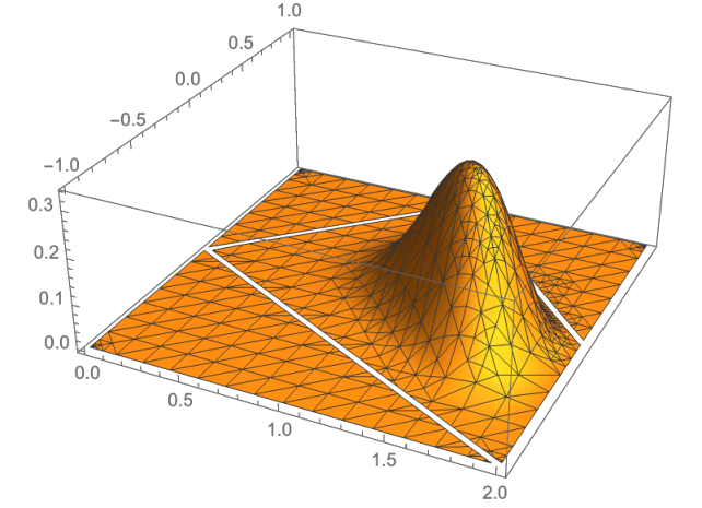


3.5 and orbits of real symmetric matrices
The case of acting on real symmetric matrices is both more challenging, since no manageable expression exists for the orbital integrals, and more intriguing, in view of the strong singularities apparent from numerical data, see Fig. 1-left.
In the case of real symmetric matrices and the action of , it is a classroom exercise to work out the PDF as a function of the differences , , . One finds
| (9) |
which exhibits an inverse–square-root singularity at the end points of its support (only the upper one if ).
In ref. [5], the case of orbits of real symmetric matrices under the action of has been treated in detail. With no loss of generality, one may assume that the matrices and are traceless. Then, to circumvent the lack of an expression for the orbital integral, it was found useful to trade the three eigenvalues (of vanishing sum) for their symmetric functions , . Write the characteristic polynomial of , with , as
For given and , and regarded as a random variable uniformly distributed in SO(3) (in the sense of Haar measure), and are also random variables, whose “PDF” may be written formally as
Parametrize in terms of Euler angles, with , and the normalized Haar measure equal to Then and are degree 2 polynomials in , so that
while the PDF for the independent variables is
| (10) |
A curious (and apparently original) identity on delta functions of polynomials then comes to the rescue:
| (11) |
where is the resultant of and , and some Jacobian. For the conditions of applicability and proof of (11), see [1].
In the present case, the resultant of and is a fairly big degree 4 polynomial of and and is a degree 1 polynomial in and , thus
| (12) | |||||
The calculation has been carried out in detail in [5] in the particular case of . Then
| (13) |
Even in that particular case, which has special symmetries, e.g. of under and of under (i.e., ), the calculation is complicated by the intricate pattern of roots of within the integration interval , and by the task of determining which of the possible zeros of give rise to a divergent integral. At the end of the day, the result reproduces very well the numerical histogram in the or in the variables, see Fig. 6.


The main merit of the expression (13) is to allow a detailed discussion of the various singularities of the integral. Divergences of can arise in two ways:
– From the vanishing of at some by coalescence of two roots of , giving rise to a non-integrable singularity of at , or
– From the overall vanishing of in some limit.
One finds a logarithmic divergence of the PDF (see eq. (10)) as approaches the blue, red and magenta lines in Fig. 7, and inverse–square-root divergences at the two special points and .
Note that because of the vanishing of the Vandermonde determinant, may have a smaller locus of singularity than , see [5].
Discussion. Though it is gratifying to have reproduced the pattern and the nature of singularities of (in a particular case, but this will generalize to arbitrary , at the price of heavier algebra), this computation sheds limited light on the geometric origin of these singularities and on what should be expected for higher . In [7] it has been argued that the singularities find their origin in the projection from the original to , and that they can be understood as arising from the singularity of certain coordinates on the product of orbits. The argument, unfortunately, says nothing about the nature of the singularity. For higher , should the singularity become softer and become just a non-analyticity like in the coadjoint cases, or should a divergence persist? Numerical experiments indicate a sharp pattern of the PDF for , but its precise nature remains elusive. There is clearly room for further progress.
4 Horn’s problem, Representation theory, and Combinatorics
In this section, we shall discuss the relationship between Horn’s problem and a basic problem in representation theory: the decomposition of tensor products of representations of a compact Lie group . The fact that multiplicities in such a decomposition admit, for large representations, a semi-classical description has been known for a long time, see [14]. More specifically, we consider here the so-called “Littlewood–Richardson (LR) multiplicities” , which appear in the decomposition of the tensor product of two irreps of highest weights and ,
| (14) |
Here we will assume that is simply connected, so that we can identify representations of and . The bottom line is that Horn’s problem appears as a semi-classical approximation of the LR multiplicities, as we will now explain.
4.1 Relation –LR
The reader may have noticed the similarity between the general form of in (8), as an integral of the product of three ’s, and the classical expression of LR multiplicities in terms of characters of the group
| (15) |
where in the second expression, the integration has been reduced to a Cartan torus . The parallel is made much tighter if one realizes that the H-C orbital integral is proportional to the character , when evaluated at , , and :
| (16) |
where has been introduced above in (5) and is the famous “Weyl denominator.” This remarkable formula reflects a deep correspondence between (“classical”) coadjoint orbits and (“quantum”) irreps of : this is the object of Kirillov’s orbit theory [18].
Using that relation, one may rewrite as expressed in (8), evaluated at a triple of h.w. shifted by , as an integral of characters. We assume that the triple is such that , where is the root lattice, since otherwise the LR multiplicity vanishes, as is well known.
The main difference between the integrals appearing in (8) and (15) is that the former runs over the whole Cartan subalgebra , while the latter is over the (compact) Cartan torus . But since , where is the coweight lattice, generated by the coweights33 3 Here the fundamental weights satisfy , while the coweights are normalized so as to satisfy . , , we may write
| (17) | |||||
Now, the sum over is a generalization of the classical identity and in general yields [10]
| (18) |
where the sum on the right runs over a finite, -independent set of weights described in [4, 7]. The coefficients are non-negative rational numbers satisfying
| (19) |
For each such term, the integral over thus yields the multiplicity . There is a similar identity involving at unshifted weights [7]. We conclude that for a triple such that , we have two identities (distinct if ):
| (20) | |||||
| (21) |
For example, for SU(3), the sum in the rhs of (18) includes only the trivial representation, so that we have simply . In contrast, for SU(4) and Spin(5) respectively,
| (22) | |||||
| (23) |
4.2 The BZ polytope, its stretching, and the function as a volume
We now change gear and introduce combinatorial methods to determine the LR coefficients. This follows from the work of Berenstein and Zelevinsky [1], who have shown that given a triple such that , one may construct a polytope , such that the LR coefficient is given by the number of integer points in . We consider this polytope as a subset of where is the number of positive roots; its dimension is at most . Then
We call the BZ polytope associated to the triple . In general it is rational but not integral (i.e. the coordinates of its vertices are rational but not always integers). Moreover, for on the interior of the support of , the dimension coincides with the degree of homogeneity of .
Determining the number of integer points in a rational polytope and its dilations is a classical problem in combinatorics. If is the dilated polytope for some positive integer , then the number of integer points in is given by the Ehrhart quasi-polynomial
where “quasi” means that the coefficients may be periodic functions of . One can prove that whenever is an integral polytope, is an honest polynomial. But there are cases where is a polynomial even though is not integral; indeed the LR stretching polynomials for are always honest polynomials even for non-integral BZ polytopes. In contrast, for the Spin groups (i.e., for the algebras), one encounters many cases of quasi-polynomiality, though we have not yet been able to discern a criterion determining which are actual polynomials.
Using standard results in combinatorics, it can be shown that the coefficient of is a constant equal to the -volume of . (In fact it is the relative volume, given by the Euclidean -volume times a scalar factor that can be computed, see [7] for details.) We now want to show that this volume is given by the function . Writing eq. (20) for a triple of dilated weights , , we have
| (24) | |||||
where in the first line we have made use of the continuity (for in ) and of the homogeneity of the function ; in the second line, for large, all the weights of the irrep of h.w. contribute additively and with their multiplicity to , and we use the relation (19).
We conclude that for large
whence
| (25) |
This vindicates the claim that the Horn problem is a semi-classical description of the LR multiplicity problem, and that the function measures the volume of the BZ polytope. Returning to the relations (20, 21) we see that they give an exact expression for this volume as a finite sum of LR multiplicities, which is more precise than the previously known asymptotic relationship.
4.3 Pictographs
This relationship between the two problems, Horn and LR, has been beautifully illustrated by the honeycomb/hive construction of Knutson and Tao [22]. KT-honeycombs are examples of pictographs, i.e., of graphical combinatorial objects that describe the two problems.
In the LR problem, the basic idea is that there should be as many (distinct) pictographs with prescribed “external labels” specifying the given three highest weights (or the three irreps) as the multiplicity itself. In other words the number of pictographs should be equal to the dimension of the space of intertwiners . KT-honeycombs are well suited for studying the Horn problem and the GL() or the multiplicity problem; their three sides are labelled by Young diagrams, i.e. by the summands of the associated integer partitions, in other words by the Young variables specifying three given irreps.
KT-honeycombs can also be used to describe multiplicities for , but in this case three other kinds of pictographs are often better suited. The pictographs that we have in mind have Dynkin labels attached to their three sides. We shall distinguish three kinds of pictographs, which look different but are essentially equivalent: the Berenstein-Zelevinsky triangles (or BZ-triangles for short), the Ocneanu blades (or O-blades) and the isometric honeycombs. The first were introduced in [2], the second in [25], and the last were discussed, in the framework of SU(3), by two of us in sect. 4 of [6]. KT-honeycombs (and hives), in relation with the solution of the Horn problem in the Hermitian case, are discussed in many places, so we shall restrict this short discussion to the case and remind the reader how the last three kinds of pictographs are related. It will be enough to present a simple example: let us consider, in SU(4), the tensor product where the indices (non-negative integers) refer to the Dynkin labels of two highest weights. The decomposition of this tensor product into a sum of irreducible representations contains terms, most of them with non-trivial multiplicity because only are inequivalent. The representation , for instance, occurs with multiplicity . This means that there will be distinct BZ-triangles with the given labels, and the same number of O-blades and -honeycombs. Fig. 8 displays one of them, in its three avatars.
.
In the BZ-triangle, the pattern of black integers is such that an integer carried by an edge is the sum of the integers labelling its end-points; the integers in blue are given (Dynkin labels). Moreover, we have one additional constraint: the red integers carried by opposite sides of hexagons are equal. In the O-blade, there is “conservation of the external integers” (Dynkin labels); we did not display the red integers: they sit in the six angles surrounding the three inner vertices, and the constraint, now, is that opposite angles (defined as the sum of their corresponding edges) should be equal. In the SU(4) honeycomb the constraint is that sums of two edges relative to opposite points of each of the three hexagons are equal.
Which pictograph one prefers is a matter of taste since the geometric correspondence between the three pictures is rather obvious. In particular the honeycomb is obtained from the O-blade by a star-triangle operation, also called a Y- transform; the constraints are automatically satisfied by displaying the hexagons of the resulting honeycomb in a metric way as parallelo-hexagons (opposite sides are parallel), or, equivalently, as equiangular hexagons (each angle has a value equal to ), because the length of each side is then given by the non-negative integer it carries.
In an equiangular hexagon, the sums of two consecutive edges surrounding opposite vertices are equal (for a proof of this elementary fact, extend the six sides of the chosen hexagon and embed the latter in one of the two resulting equilateral triangles). Remember also that the black integers are non-negative, but they are allowed to equal , in which case the irregular hexagons may degenerate to pentagons or to quadrilaterals. For , there are inner vertices in the O-blades (the same as the number of hexagons), and we can intuitively interpret the existence of some non-trivial multiplicity relative to a chosen triple of irreps as a kind of “breathing” of the (irregular) hexagons. More properties of O-blades and isometric honeycombs, in particular their decomposition on “fundamental pictographs,” can be found in [6]. Notice that the external sides of the KT-honeycombs are labelled by partitions, whereas those of the isometric honeycombs are labelled by Dynkin indices. Moreover the numbers carried by the leaves (internal edges) are non-negative integers in the latter case, whereas they can be negative in the former (which cannot be “isometric,” of course). For purposes of illustration, Fig. 9 displays an isometric honeycomb for a triple of highest weights with rather large entries.
Although one can construct BZ polytopes for all simple Lie groups, pictographs have been invented only for . Finding analogs of the latter for other types of simple Lie group is a problem that has baffled the community and is still waiting for an answer.
4.4 Relation with symmetric polynomials
Since characters of representations combine multiplicatively under the tensor product, the multiplicities can be interpreted as structure constants in the ring of symmetric functions generated by the characters of the irreps of . In the case of for example, these multiplicities encode the structure constants for the Schur polynomials.
In the coadjoint case, we have a notion of BZ polytopes (and, in the subcase, we also have pictographs); we know that the volume of a BZ-polytope is measured by the value of the function, a value that can be obtained by looking at the highest degree coefficient of the stretching (or LR) polynomial when multiplicities are scaled. Moreover, we have an equality between structure constants of the algebra of symmetric polynomials in the Schur basis and the number of integer points of appropriate BZ-polytopes (or hive polytopes), for . We obtain therefore a relation between the function , as defined in the (Hermitian) Horn problem, and the scaling behavior of appropriate structure constants of the ring of symmetric polynomials in the Schur basis. Clearly this kind of relation extends to other situations, where the Lie group is replaced by other simple Lie groups and where Schur polynomials are replaced by orthogonal Schur polynomials, symplectic Schur polynomials, etc.
In the self-adjoint case, however, there is no obvious notion of multiplicity and there are no BZ-polytopes. Nevertheless, we still have a function stemming from the Horn problem. Could this function be related to some kind of volume, or to some kind of asymptotic behavior for the structure constants of an appropriate class of polynomials? The answer to the second part of the question is positive: as discussed in [5], one shows that for or 2, is the limit of the structure constants of appropriate zonal polynomials (Jack polynomials with parameter ), see also [26]. The approach to asymptotics is illustrated in Fig. 10 which displays both the volume function , calculated from the integral of eq. (12), for some choice of its arguments, and a vertically scaled version of the surface approximating the corresponding44 4 See [5] for more details. zonal structure constants.


Middle : Point plot of the volume function for the corresponding arguments.
Right: Superposition of both.
Remark : Because of the large vertical coordinate range, those parts of the surface lying far from the singularities look essentially flat and one only sees the singularities (high values of ).
The answer to the first part of the question is not known: notice that there is no clear way to obtain a combinatorial interpretation of a would-be hive or BZ-polytope, since the structure constants of zonal polynomials are usually not integers but rational numbers — they are integers if the Jack parameter , but this is because one recovers in that case the Schur polynomials themselves! We leave this problem to the sagacity of our readers.
Acknowledgements
The work of Colin McSwiggen is partially supported by the National Science Foundation under Grant No. DMS 1714187, as well as by the Chateaubriand Fellowship of the Embassy of France in the United States.
References
- [1] M. Bauer and J.-B. Zuber, On products of delta distributions and resultants, to appear
- [2] A. Berenstein and A. Zelevinsky, Triple multiplicities for and the spectrum of the exterior algebra of the adjoint representation, J. Alg. Combin. 1 (1992) 7–22
- [3] É. Brézin and S. Hikami, An extension of the Harish-Chandra–Itzykson–Zuber integral, http://arxiv.org/abs/math-ph/0208002v1; WKB-expansion of the Harish-Chandra–Itzykson–Zuber integral for arbitrary , Progress of Theoretical Physics, 116 (2006) 441–502, http://arxiv.org/abs/math-ph/0604041v1
- [4] R. Coquereaux and J.-B. Zuber, From orbital measures to Littlewood–Richardson coefficients and hive polytopes, Ann. Inst. Henri Poincaré Comb. Phys. Interact., 5 (2018) 339–386, http://arxiv.org/abs/1706.02793
- [5] R. Coquereaux and J.-B. Zuber, The Horn Problem for Real Symmetric and Quaternionic Self-Dual Matrices, SIGMA 15 (2019) 029, http://arxiv.org/abs/1809.03394
- [6] R. Coquereaux and J.-B. Zuber, Conjugation properties of tensor product multiplicities, J. Phys. A: Math. Theor. 47 (2014) 455202 (28pp) doi:10.1088/1751-8113/47/45/455202 http://arxiv.org/abs/1405.4887
- [7] R. Coquereaux, C. McSwiggen and J.-B. Zuber, On Horn’s Problem and its Volume Function, http://arxiv.org/abs/1904.00752
- [8] J. Day, W. So and R. C. Thompson, The spectrum of a Hermitian matrix sum, Linear Algebra and its Applications 280 (1998) 289–332
- [9] A.H. Dooley, J. Repka and N. Wildberger, Sums of Adjoint Orbits, Linear and Multilinear Algebra (1993), 36, 79–101
- [10] P. Etingof and E. Rains, Mittag–Leffler type sums associated with root systems, http://arxiv.org/abs/1811.05293
- [11] J. Faraut, Horn’s problem, and Fourier analysis, Tunisian Journal of Mathematics, 1 (2019) 585–606
- [12] W. Fulton, Eigenvalues, invariant factors, highest weights, and Schubert calculus, Bull. Amer. Math. Soc. 37 (2000), 209–249, http://arxiv.org/abs/math/9908012
- [13] Harish-Chandra, Differential Operators on a Semisimple Algebra, Amer. J. Math. 79 (1957) 87–120
- [14] G.J. Heckman, Projections of Orbits and Asymptotic Behavior of Multiplicities for Compact Connected Lie Groups, Invent. Math. 67 (1982), 333–356
- [15] A. Horn, Doubly stochastic matrices and the diagonal of a rotation matrix, Amer. J. Math. 76 (1954), 620–630
- [16] A. Horn, Eigenvalues of sums of Hermitian matrices, Pacific J. Math. 12 (1962), 225–241
- [17] C. Itzykson and J.-B. Zuber, The planar approximation II, J. Math. Phys. 21 (1980) 411–421
- [18] A.A. Kirillov, Lectures on the Orbit Method. American Mathematical Society, Providence (2004)
- [19] A.A. Klyachko, Stable bundles, representation theory and Hermitian operators, Selecta Math. (N.S.) 4 (1998), 419–445
- [20] A. Knutson, The symplectic and algebraic geometry of Horn’s problem, Linear Algebra Appl. 319 (2000), 61–81
- [21] A. Knutson and T. Tao, Honeycombs and sums of Hermitian matrices, Notices Amer. Math. Soc. 48 (2001), 175–186, http://arxiv.org/abs/math/0009048
- [22] A. Knutson, T. Tao, The honeycomb model of GL(n) tensor products I: Proof of the saturation conjecture, J. Amer. Math. Soc. 12 (1999), 1055–1090, http://arxiv.org/abs/math/9807160
- [23] Mathematica, Wolfram Research, Inc., Champaign, IL, 2012, http://www.wolfram.com/
- [24] C. McSwiggen, A new proof of Harish-Chandra’s integral formula, Commun. Math. Phys. 365 (2019), 239–253, http://arxiv.org/abs/1712.03995
- [25] A. Ocneanu, Various conferences and private communication (2009).
- [26] A. Okounkov, G. Olshanski, Shifted Jack polynomials, binomial formula, and applications, Math. Res. Lett. 4 (1997), 69–78, http://arXiv.org/abs/q-alg/9608020
- [27] H. Weyl, Das asymptotische Verteilungsgesetz der Eigenwerte linearer partieller Differentialgleichungen, Math. Ann. 71 (1912), 441–479
- [28] J.-B. Zuber, Horn’s problem and Harish-Chandra’s integrals. Probability distribution functions, Ann. Inst. Henri Poincaré Comb. Phys. Interact., 5 (2018), 309-338, http://arxiv.org/abs/1705.01186