跳到论文正文
W Papers独立论文阅读器 arXiv:1905.09599 论文正文 计算阅读时间 · 0%
引用这篇论文根据当前论文元数据生成,正式投稿前建议核对。


License: arXiv.org perpetual non-exclusive license
arXiv:1905.09599v1 [math.ST] 23 May 2019

On generalized Piterbarg-Berman function

Chengxiu Ling Address: Chengxiu Ling, Department of Mathematical Sciences, Xi’an Jiaotong-Liverpool University, Suzhou 215123, China Email address: chengxiu.ling@xjtlu.edu.cn , Hong Zhang Address: Hong Zhang, School of Mathematics and Statistics, Southwest University, Chongqing 400715, China Email address: crystal1994@email.swu.edu.cn and Long Bai Address: Long Bai, Department of Mathematical Sciences, Xi’an Jiaotong-Liverpool University, Suzhou 215123, China Email address: long.bai@xjtlu.edu.cn
Date: August 11, 2026
Abstract.

This paper aims to evaluate the Piterbarg-Berman function given by

𝒫ℬαh(x,E)=∫ℝezℙ{∫E𝕀(2Bα(t)−|t|α−h(t)−z>0)dt>x}dz,x∈[0,mes(E)],\mathcal{P\!B}_{\alpha}^{h}(x,E)=\int_{\mathbb{R}}e^{z}\mathbb{P}\left\{\int_{E}\mathbb{I}\left(\sqrt{2}B_{\alpha}(t)-|t|^{\alpha}-h(t)-z>0\right)\text{\rm d}t>x\right\}\text{\rm d}z,\hskip 8.50012ptx\in[0,{mes}(E)],

with hh a drift function and BαB_{\alpha} a fractional Brownian motion (fBm) with Hurst index α/2∈(0,1]\alpha/2\in(0,1], i.e., a mean zero Gaussian process with continuous sample paths and covariance function

Cov⁡(Bα​(s),Bα​(t))=12​(|s|α+|t|α−|s−t|α).\displaystyle\mathrm{Cov}(B_{\alpha}(s),B_{\alpha}(t))=\frac{1}{2}(|s|^{\alpha}+|t|^{\alpha}-|s-t|^{\alpha}).

This note specifies its explicit expression for the fBms with α=1\alpha=1 and 22 when the drift function h⁡(t)=c​tα,c>0h(t)=ct^{\alpha},c>0 and E=ℝ+∪{0}E=\mathbb{R}_{+}\cup\{0\}. For the Gaussian distribution B2B_{2}, we investigate 𝒫​ℬ2h​(x,E)\mathcal{P\!B}_{2}^{h}(x,E) with general drift function h⁡(t)h(t) such that h⁡(t)+t2h(t)+t^{2} being convex or concave, and finite interval E=[a,b]E=[a,b]. Typical examples of 𝒫​ℬ2h​(x,E)\mathcal{P\!B}_{2}^{h}(x,E) with h⁡(t)=c​|t|λ−t2h(t)=c\left\lvert t\right\rvert^{\lambda}-t^{2} and several bounds of 𝒫​ℬαh​(x,E)\mathcal{P\!B}_{\alpha}^{h}(x,E) are discussed. Numerical studies are carried out to illustrate all the findings.

Keywords: Piterbarg-Berman function; sojourn time; fractional Brownian motion; drift function

AMS Classification: Primary 60G15; secondary 60G70

1. Introduction

Consider a centered Gaussian process {X⁡(t),t∈ℝ}\{X(t),\,t\in\mathbb{R}\} with càdlàd sample paths and let for T>0T>0

Lu,T:=∫0T𝕀⁡(X⁡(t)>u)​d​t\displaystyle L_{u,T}:=\int_{0}^{T}\mathbb{I}\left(X\left(t\right)>u\right)\text{\rm d}t

be the sojourn time of XX above the level u∈ℝu\in\mathbb{R} during the observed period [0,T][0,T], where 𝕀⁡(⋅)\mathbb{I}\left(\cdot\right) stands for the indicator function. In a series of papers culminating in [1], S. Berman derived results on the tail asymptotic behavior of ν⁡(u)​Lu,T\nu(u)L_{u,T} with an appropriate scaling function ν⁡(u)\nu(u) such that

(1.1) pu,T(x)=ℙ{ν(u)Lu,T>x}∼C(x)ℙ{supt∈[0,T]X(t)>u}\displaystyle p_{u,T}(x)=\mathbb{P}\left\{\nu(u)L_{u,T}>x\right\}\sim C(x)\mathbb{P}\left\{\sup_{t\in[0,T]}X(t)>u\right\}

as u→∞u\to\infty. This essentially builds a bridge of asymptotic behavior of the sojourn time Lu,TL_{u,T} and the extremal analysis of the Gaussian processes via the link function C⁡(x)C(x). However, the asymptotic function CC is in general difficult to obtain except very few special processes and approximations have been suggested to evaluate. A related work is given by [2] for a standard Brownian motion with linear drift function. For a stationary and standard Gaussian process XX with correlation function ρ\rho satisfies the Pickands’ assumption ρ⁡(t)=1−|t|α​[1+o⁡(1)],α∈(0,2]\rho(t)=1-|t|^{\alpha}[1+o(1)],\alpha\in(0,2] for small |t||t|, [1] showed an explicit form of function CC via the following tail distribution (see Theorem 3.3.1 therein)

(1.2) G(x)=ℙ{∫ℝ𝕀(2Bα(t)−|t|α+𝒲>0)dt>x},x≥0,\displaystyle G(x)=\mathbb{P}\left\{\int_{\mathbb{R}}\mathbb{I}(\sqrt{2}B_{\alpha}(t)-|t|^{\alpha}+\mathcal{W}>0)\text{\rm d}t>x\right\},\quad x\geq 0,

where 𝒲\mathcal{W} is a standard exponential distributed random variable, independent of BαB_{\alpha}, a fractional Brownian motion (fBm) with Hurst index α/2∈(0,1]\alpha/2\in(0,1], i.e., a mean zero Gaussian process with continuous sample paths and covariance function

Cov⁡(Bα​(s),Bα​(t))=12​(|s|α+|t|α−|s−t|α).\displaystyle\mathrm{Cov}(B_{\alpha}(s),B_{\alpha}(t))=\frac{1}{2}(|s|^{\alpha}+|t|^{\alpha}-|s-t|^{\alpha}).

The recent contribution [3] discussed (1.1) and gave the approximations of the related sojourn time of discrete form for locally stationary Gaussian processes, and [4] investigated general Gaussian processes with strictly positive drift function. For more related discussions on ruin time and the extremal analysis of Gaussian processes and random fields in financial and insurance framework, we refer to [5, 6, 7, 8, 9, 10, 11, 12, 13, 14].

Motivated by the importance of the crucial function arising in the extremal behavior of the sojourn time and the random processes involved, this paper studies thus a general form of function GG given in (1.2). Precisely, define for a compact set EE in ℝ\mathbb{R} and a continuous drift function hh on EE

(1.3) 𝒫ℬαh(x,E):=∫ℝezℙ{∫E𝕀(2Bα(t)−|t|α−h(t)−z>0)dt>x}dz,x∈[0,mes(E)]\displaystyle\qquad\mathcal{P\!B}_{\alpha}^{h}(x,E):=\int_{\mathbb{R}}e^{z}\mathbb{P}\left\{\int_{E}\mathbb{I}(\sqrt{2}B_{\alpha}(t)-|t|^{\alpha}-h(t)-z>0)\text{\rm d}t>x\right\}\text{\rm d}z,\quad x\in[0,\mathrm{mes}(E)]

and

(1.4) 𝒫​ℬαh​(x):=limT→∞𝒫​ℬαh​(x,[0,T])T𝕀⁡(h=0),x≥0\displaystyle\mathcal{P\!B}_{\alpha}^{h}(x):=\lim_{T\to\infty}\frac{\mathcal{P\!B}_{\alpha}^{h}(x,[0,T])}{T^{\mathbb{I}\left(h=0\right)}},\quad x\geq 0

provided that the above integral and limits exist. For h=0h=0, we suppress the superscript and write 𝒫​ℬα​(x)\mathcal{P\!B}_{\alpha}(x) or 𝒫​ℬα​(x,E)\mathcal{P\!B}_{\alpha}(x,E). Typical examples of the function 𝒫​ℬαh​(x,E)\mathcal{P\!B}_{\alpha}^{h}(x,E) can be found in [3] for h=0,E=ℝh=0,E=\mathbb{R}, and [4] for polynomial function hh and general interval EE.

Clearly, our setting is very common since 𝒫​ℬα​(0)\mathcal{P\!B}_{\alpha}(0) is simply the Pickands’ constant, which values are known only for α=1,2\alpha=1,2, i.e., 𝒫​ℬ1​(0)=1,𝒫​ℬ2​(0)=1/π\mathcal{P\!B}_{1}(0)=1,\mathcal{P\!B}_{2}(0)=1/\sqrt{\pi}, see e.g., [15, 16, 17, 18, 19, 20, 21, 22, 23, 24, 25, 26] for related studies on its expressions and bounds, while 𝒫​ℬαh​(0)\mathcal{P\!B}_{\alpha}^{h}(0) reduces to the Piterbarg constants for strictly positive drift function. The recent contribution [27] studied the basic properties of the generalized Piterbarg constant 𝒫​ℬαh​(0){\mathcal{P\!B}}_{\alpha}^{h}(0) for power drift function, which are available for all α∈(0,2]\alpha\in(0,2]. For more general studies on sojourn sets with moving boundary of the processes involved and applications in physics and finance fields, we refer to [28] and among others.

The first result below is concerned with the explicit expression of 𝒫​ℬαh​(x,E)\mathcal{P\!B}_{\alpha}^{h}(x,E) for the standard Brownian motion and Gaussian distribution, i.e., the fBm with α=1\alpha=1 and α=2\alpha=2. Here, we focus simply on E=ℝ+∪{0}E=\mathbb{R}_{+}\cup\{0\} and positive drift function h⁡(t)=c​tα,t≥0,c>0h(t)=ct^{\alpha},t\geq 0,c>0. In what follows, let Ψ⁡(⋅)\Psi(\cdot) and φ⁡(⋅)\varphi(\cdot) be the survival function and probability density function of 𝒩∼N⁡(0,1)\mathcal{N}\sim N(0,1), respectively.

Theorem 1.1.

Let 𝒫​ℬαh​(x){\mathcal{P\!B}}_{\alpha}^{h}(x) be the Piterbarg-Berman function given by (1.3) with drift function h⁡(t)=c​tα,t≥0,c>0h(t)=ct^{\alpha},t\geq 0,c>0. We have with xc=(1+c)​x/2x_{c}=(1+c)\sqrt{x/2} and xc′=(1−c)​x/2x_{c}^{\prime}=(1-c)\sqrt{x/2}

𝒫​ℬ1h​(x)\displaystyle{\mathcal{P\!B}}_{1}^{h}(x) =(1+c)2cΨ(xc)−(1−c)xcφ(xc)+[(1−c)24​(1+c)xc2+1+c2]e−xc2/2\displaystyle=\frac{(1+c)^{2}}{c}\Psi(x_{c})-(1-c)x_{c}\varphi(x_{c})+\left[\frac{(1-c)^{2}}{4(1+c)}x_{c}^{2}+\frac{1+c}{2}\right]e^{-x_{c}^{2}/2}
−(1+c)e−c​x[1−ccΨ(xc′)−xc′φ(xc′)+1+xc′2/22e−xc′2/2]\displaystyle\quad-(1+c)e^{-cx}\left[\frac{1-c}{c}\Psi(x_{c}^{\prime})-x_{c}^{\prime}\varphi(x_{c}^{\prime})+\frac{1+x_{c}^{\prime 2}/2}{2}e^{-x_{c}^{\prime 2}/2}\right]

and

𝒫​ℬ2h​(x)=1+cc​Ψ​(c⁡(1+c)2​x)​e−(1+c)​x24+Ψ⁡(1−c2​x)​e−c​x2−Ψ⁡(1+c2​x),x≥0.\displaystyle{\mathcal{P\!B}}_{2}^{h}(x)=\sqrt{\frac{1+c}{c}}\Psi\left(\sqrt{\frac{c(1+c)}{2}}x\right)e^{-\frac{(1+c)x^{2}}{4}}+\Psi\left(\frac{1-c}{\sqrt{2}}x\right)e^{-cx^{2}}-\Psi\left(\frac{1+c}{\sqrt{2}}x\right),\quad x\geq 0.
Remark 1.2.

The explicit expression of 𝒫​ℬ1h​(x){\mathcal{P\!B}}_{1}^{h}(x) is obtained by the considerable analysis of the stopping time and the random sojourn time involved:

(1.5) τz=inf{t≥0:2​B1​(t)−t−h⁡(t)≥z},Yz=∫0∞𝕀⁡(2​B1​(t)−t−h⁡(t)−z>0)​d​t,\displaystyle\tau_{z}=\inf\{t\geq 0:\sqrt{2}B_{1}(t)-t-h(t)\geq z\},\quad Y_{z}=\int_{0}^{\infty}\mathbb{I}(\sqrt{2}B_{1}(t)-t-h(t)-z>0)\text{\rm d}t,

which nice properties are referred to [29] due to the linear drift function. The general case with non-linear drift function and finite time interval is an open question and it may require definite efforts to develop the initial properties of τz\tau_{z} and YzY_{z} involved.

The main methodology for the establishment of 𝒫​ℬ2h​(x){\mathcal{P\!B}}_{2}^{h}(x) above is essentially determined by the convex curve family f𝒩​(t)=f𝒩​(t,z),z∈ℝf_{\mathcal{N}}(t)=f_{\mathcal{N}}(t,z),z\in\mathbb{R} (recall (1.3))

(1.6) f𝒩​(t)=h⁡(t)+t2−2​𝒩​t+z,t∈ℝ\displaystyle f_{\mathcal{N}}(t)=h(t)+t^{2}-\sqrt{2}\mathcal{N}t+z,\quad t\in\mathbb{R}

since h⁡(t)=c​t2h(t)=ct^{2} and B2​(t)=𝒩​t,t∈ℝB_{2}(t)=\mathcal{N}t,\,t\in\mathbb{R}. In the following theorem, we consider a general drift function hh such that h⁡(t)+t2h(t)+t^{2} is convex on E/ℝ{E/\mathbb{R}}, which leads equivalently that f𝒩​(t)f_{\mathcal{N}}(t) is continuous and convex on E/ℝE/\mathbb{R}. Let thus s1<s2s_{1}<s_{2} and t1<t2t_{1}<t_{2} be the two random solutions of f𝒩​(s)=0,s∈Ef_{\mathcal{N}}(s)=0,\,s\in E and f𝒩​(t)=0,t∈ℝf_{\mathcal{N}}(t)=0,t\in\mathbb{R}, respectively if it holds that

f𝒩​(s∗)=mins∈E⁡f𝒩​(s)<0,f𝒩​(t∗)=mint∈ℝ⁡f𝒩​(t)<0.\displaystyle f_{\mathcal{N}}(s^{*})=\min_{s\in E}f_{\mathcal{N}}(s)<0,\quad f_{\mathcal{N}}(t^{*})=\min_{t\in\mathbb{R}}f_{\mathcal{N}}(t)<0.
Theorem 1.3.

Let 𝒫​ℬαh​(x,E)\mathcal{P\!B}_{\alpha}^{h}(x,E) be given by (1.3) with E=[a,b],a<b,a,b∈ℝE=[a,b],a<b,a,b\in\mathbb{R}.

(i) If h⁡(t)+t2h(t)+t^{2} is a continuous, convex function on EE, then

𝒫ℬ2h(x,E)=∫ℝez[ℙ{f𝒩(a)<0,f𝒩(b)<0}dz+ℙ{f𝒩(a)>0,f𝒩(b)>0,s2−s1>x,f𝒩(s∗)<0}]dz\displaystyle\mathcal{P\!B}_{2}^{h}(x,E)=\int_{\mathbb{R}}e^{z}\left[\mathbb{P}\left\{f_{\mathcal{N}}(a)<0,f_{\mathcal{N}}(b)<0\right\}\text{\rm d}z+\mathbb{P}\left\{f_{\mathcal{N}}(a)>0,f_{\mathcal{N}}(b)>0,s_{2}-s_{1}>x,f_{\mathcal{N}}(s^{*})<0\right\}\right]\text{\rm d}z
+∫ℝez[ℙ{f𝒩(a)≤0,f𝒩(a+x)<0,f𝒩(b)>0}+ℙ{f𝒩(a)>0,f𝒩(b−x)<0,f𝒩(b)≤0}]dz.\displaystyle\quad+\int_{\mathbb{R}}e^{z}\left[\mathbb{P}\left\{f_{\mathcal{N}}(a)\leq 0,f_{\mathcal{N}}(a+x)<0,f_{\mathcal{N}}(b)>0\right\}+\mathbb{P}\left\{f_{\mathcal{N}}(a)>0,f_{\mathcal{N}}(b-x)<0,f_{\mathcal{N}}(b)\leq 0\right\}\right]\text{\rm d}z.

(ii) If h⁡(t)+t2,t∈ℝh(t)+t^{2},t\in\mathbb{R} is continuous and convex, and the finite right derivative h+′​(a)h^{\prime}_{+}(a) and the left derivative h−′​(b)h^{\prime}_{-}(b) exist with finite values, then h+′​(a)≤h−′​(b)h^{\prime}_{+}(a)\leq h^{\prime}_{-}(b) and

𝒫​ℬ2h​(x,E)=∫ℝez​[ℙ⁡{f𝒩​(a+x)<0,2​𝒩≤h+′​(a)+2​a}+ℙ⁡{f𝒩​(b−x)<0,2​𝒩≥h−′​(b)+2​b}]​d​z\displaystyle\mathcal{P\!B}_{2}^{h}(x,E)=\int_{\mathbb{R}}e^{z}\left[\mathbb{P}\left\{f_{\mathcal{N}}(a+x)<0,\sqrt{2}\mathcal{N}\leq h^{\prime}_{+}(a)+2a\right\}+\mathbb{P}\left\{f_{\mathcal{N}}(b-x)<0,\sqrt{2}\mathcal{N}\geq h^{\prime}_{-}(b)+2b\right\}\right]\text{\rm d}z
+∫ℝezℙ{min(b,t2)−max(a,t1)>x,h+′(a)+2a<2𝒩<h−′(b)+2b,f𝒩(t∗)<0}dz.\displaystyle\quad+\int_{\mathbb{R}}e^{z}\mathbb{P}\left\{\min(b,t_{2})-\max(a,t_{1})>x,h^{\prime}_{+}(a)+2a<\sqrt{2}\mathcal{N}<h^{\prime}_{-}(b)+2b,f_{\mathcal{N}}(t^{*})<0\right\}\text{\rm d}z.

Typical examples of Theorem 1.3 are discussed in Propositions 2.1 and 2.2 where we take h⁡(t)=c​|t|λ−t2h(t)=c|t|^{\lambda}-t^{2} with λ=1,2\lambda=1,2 and all λ≥1\lambda\geq 1. Some bounds are also specified in Proposition 2.3. All alternative results for hh such that h⁡(t)+t2h(t)+t^{2} is concave are established, see Theorem 5.1, Propositions 5.1 and 5.2 in Appendix 5.

The study on 𝒫​ℬαh\mathcal{P\!B}_{\alpha}^{h} for fBms BαB_{\alpha} with general α∈(0,1)∪(1,2)\alpha\in(0,1)\cup(1,2) is still open since the Slepian’s inequality for extremes of processes is not applicable in the sojourn times setting, see e.g., [13].

The rest of this paper is organized as follows. Section 2 gives several typical examples and its bounds as well. Section 3 carries out a small scale of numerical studies to illustrate the findings. All proofs are relegated to Section 4. We present Appendix 5 for 𝒫​ℬ2h\mathcal{P\!B}_{2}^{h} with concave drift functions.

2. Further Discussions and Applications

Clearly, a straightforward application of Theorem 1.3 with h⁡(t)=c​|t|λ−t2,t∈ℝ,c>0,λ≥1h(t)=c|t|^{\lambda}-t^{2},\,t\in\mathbb{R},c>0,\lambda\geq 1 implies the explicit expressions of 𝒫​ℬ2h\mathcal{P\!B}_{2}^{h}, which are given in Proposition 2.1 and 2.2 for λ=1,2\lambda=1,2 and λ≥1\lambda\geq 1. Some bounds are derived in Proposition 2.3 for 𝒫​ℬ2h\mathcal{P\!B}_{2}^{h}.

2.1. Explicit expressions of 𝒫​ℬ2h​(x,E)\mathcal{P\!B}_{2}^{h}(x,E) with h⁡(t)=c​|t|λ−t2h(t)=c|t|^{\lambda}-t^{2}

Recalling that f𝒩​(t)=h⁡(t)+t2−2​𝒩​t+z=f−𝒩​(−t)f_{\mathcal{N}}(t)=h(t)+t^{2}-\sqrt{2}\mathcal{N}t+z=f_{-\mathcal{N}}(-t) for symmetry hh implies that for the sojourn time ℒ𝒩​(z)=∫ab𝕀⁡(f𝒩​(t)<0)​d​t\mathcal{L}_{\mathcal{N}}(z)=\int_{a}^{b}\mathbb{I}(f_{\mathcal{N}}(t)<0)\text{\rm d}t

𝒫ℬ2h(x,[a,b])=∫ℝezℙ{ℒ𝒩(z)>x}dz=𝒫ℬ2h(x,[−b,−a]),x∈[0,b−a].\displaystyle\mathcal{P\!B}_{2}^{h}(x,[a,b])=\int_{\mathbb{R}}e^{z}\mathbb{P}\left\{\mathcal{L}_{\mathcal{N}}(z)>x\right\}\text{\rm d}z=\mathcal{P\!B}_{2}^{h}(x,[-b,-a]),\quad x\in[0,b-a].

We consider only E=[a,b]E=[a,b] with b>0b>0 unless stated otherwise.

Proposition 2.1.

Let 𝒫​ℬ2h​(x,E)\mathcal{P\!B}_{2}^{h}(x,E) be the Piterbarg-Berman function defined in (1.3) with h⁡(t)=c​|t|λ−t2,c>0h(t)=c|t|^{\lambda}-t^{2},c>0 and E=[a,b]E=[a,b]. Denote by f𝒩​(t)=c​|t|λ−2​𝒩​t+z,𝒩∼N⁡(0,1)f_{\mathcal{N}}(t)=c|t|^{\lambda}-\sqrt{2}\mathcal{N}t+z,\,\mathcal{N}\sim N(0,1) as in (1.6).

(i) For λ=2\lambda=2, we have

𝒫ℬ2h(x,E)=∫ℝez[ℙ{f𝒩(a+x)<0,2𝒩/c<2a+x}+ℙ{f𝒩(b−x)<0,2𝒩/c>2b−x}]dz\displaystyle{\mathcal{P\!B}_{2}^{h}(x,E)}=\small\int_{\mathbb{R}}e^{z}\left[\mathbb{P}\left\{f_{\mathcal{N}}(a+x)<0,\sqrt{2}\mathcal{N}/c<{2a+x}\right\}+\mathbb{P}\left\{f_{\mathcal{N}}(b-x)<0,\sqrt{2}\mathcal{N}/c>{2b-x}\right\}\right]\text{\rm d}z
+∫ℝezℙ{2𝒩2/c2>x2+4z/c, 2a+x<2𝒩/c<2b−x}dz\displaystyle\small+\int_{\mathbb{R}}e^{z}\mathbb{P}\left\{2\mathcal{N}^{2}/c^{2}>{x^{2}+4z/c},\,{2a+x}<{\sqrt{2}}\mathcal{N}/c<{2b-x}\right\}\text{\rm d}z\hskip 18.49988pt\hskip 18.49988pt\hskip 18.49988pt\hskip 18.49988pt

and for h≡0h\equiv 0,i.e., c=1c=1

𝒫​ℬ2​(x,[0,T])=2​Ψ​(x/2)+2​(T−x)​φ​(x/2),𝒫​ℬ2​(x)=limT→∞𝒫​ℬ2​(x,[0,T])T=2​φ​(x/2).\displaystyle\mathcal{P\!B}_{2}(x,[0,T])=2\Psi(x/\sqrt{2})+\sqrt{2}(T-x)\varphi(x/\sqrt{2}),\quad\mathcal{P\!B}_{2}(x)=\lim_{T\to\infty}\frac{\mathcal{P\!B}_{2}(x,[0,T])}{T}=\sqrt{2}\varphi(x/\sqrt{2}).

(ii) For λ=1\lambda=1, we have with ν⁡(m,c)=em2−c​|m|​Ψ​([c−2​m]/2)\nu(m,c)=e^{m^{2}-c|m|}\Psi\left([c-2m]/{\sqrt{2}}\right)

𝒫​ℬ2h​(x,E)={e(a+x)​(a+x−c)−ν⁡(a+x,c)+ν⁡(b−x,c),a≥0,ν(b−x,c)+ν(−(a+x),c)+∫−∞0ezℙ{2|𝒩|<c,min(b,t2)−max(a,t1)>x}dz,a<0,\displaystyle\mathcal{P\!B}_{2}^{h}(x,{E})=\small\left\{\begin{array}[]{ll}e^{(a+x)(a+x-c)}-\nu(a+x,c)+\nu(b-x,c),&a\geq 0,\\ \nu(b-x,c)+\nu(-(a+x),c)+\int_{-\infty}^{0}e^{z}\mathbb{P}\left\{\sqrt{2}|\mathcal{N}|<c,\min(b,t_{2})-\max(a,t_{1})>x\right\}\text{\rm d}z,&a<0,\end{array}\right.

where t1<t2t_{1}<t_{2} are as in Theorem 1.3 (ii), i.e., the random solutions of f𝒩​(t)=0,t∈ℝf_{\mathcal{N}}(t)=0,\,t\in\mathbb{R} equal

t1=zc+2​𝒩<0<−zc−2​𝒩=t2,z<0.\displaystyle t_{1}=\frac{z}{c+\sqrt{2}\mathcal{N}}<0<\frac{-z}{c-\sqrt{2}\mathcal{N}}=t_{2},\quad z<0.

Intuitively, the three parts involved for λ=2\lambda=2 above are obtained via the comparison among the symmetric axis t=2​𝒩/(2​c)t=\sqrt{2}\mathcal{N}/(2c) of the quadratic symmetric curve f𝒩​(⋅)f_{\mathcal{N}}(\cdot), a+x/2a+x/2 and b−x/2b-x/2. Meanwhile, the well-known Pickands’ constant 𝒫​ℬ2​(0)=π\mathcal{P\!B}_{2}(0)=\sqrt{\pi} can be implied by 𝒫​ℬ2​(x)=2​φ​(x),x≥0\mathcal{P\!B}_{2}(x)=\sqrt{2}\varphi(x),x\geq 0. The specification for λ=1\lambda=1 follows from Theorem 1.3 (ii), and the expression of 𝒫​ℬ2h​(x,E)\mathcal{P\!B}_{2}^{h}(x,E) with E=[a,b]E=[a,b] including the original point is more involved due to the piece-wise property of f𝒩​(⋅)f_{\mathcal{N}}(\cdot). Its detailed expansions are given in Appendix 5.2. Below, we consider the general drift function h⁡(t)=c​|t|λ−t2h(t)=c|t|^{\lambda}-t^{2} with λ≥1\lambda\geq 1. The case with 0<λ<10<\lambda<1 is given in Proposition 5.1 in Appendix 5.1.

Proposition 2.2.

Let 𝒫​ℬ2h​(x,E)\mathcal{P\!B}_{2}^{h}(x,E) be the Piterbarg-Berman function defined in (1.3) with drift function h⁡(t)=c​|t|λ−t2,c>0,λ≥1h(t)=c|t|^{\lambda}-t^{2},c>0,\lambda\geq 1 and E=[a,b]E=[a,b].

(i) For a≥0a\geq 0, we have

𝒫​ℬ2h​(x,E)=𝔼⁡{𝕀⁡(2​𝒩​(a+x)+𝒲>c​(a+x)λ)}\displaystyle\mathcal{P\!B}_{2}^{h}(x,E)=\mathbb{E}\left\{\mathbb{I}(\sqrt{2}\mathcal{N}(a+x)+\mathcal{W}>c(a+x)^{\lambda})\right\}
+∫0∞ezℙ{min(b,t2)−max(a,t1)>x,f𝒩(t∗)<0,𝒩>0}dz.\displaystyle\quad+\int_{0}^{\infty}e^{z}\mathbb{P}\left\{\min(b,t_{2})-\max(a,t_{1})>x,f_{\mathcal{N}}(t^{*})<0,\mathcal{N}>0\right\}\text{\rm d}z.

(ii) For a<0a<0, we have

𝒫​ℬ2h​(x,E)=∫ℝez​[ℙ⁡{f𝒩​(a+x)<0,f𝒩′​(a)≥0}+ℙ⁡{f𝒩​(b−x)<0,f𝒩′​(b)≤0}]​d​z\displaystyle\mathcal{P\!B}_{2}^{h}(x,E)=\int_{\mathbb{R}}e^{z}\left[\mathbb{P}\left\{f_{\mathcal{N}}(a+x)<0,f_{\mathcal{N}}^{\prime}(a){\geq}0\right\}+\mathbb{P}\left\{f_{\mathcal{N}}(b-x)<0,f_{\mathcal{N}}^{\prime}(b){\leq}0\right\}\right]\text{\rm d}z
+∫ℝezℙ{min(b,t2)−max(a,t1)>x,f𝒩′(a)<0<f𝒩′(b),f𝒩(t∗)<0}dz.\displaystyle\quad+\int_{\mathbb{R}}e^{z}\mathbb{P}\left\{\min(b,t_{2})-\max(a,t_{1})>x,f_{\mathcal{N}}^{\prime}(a)<0<f_{\mathcal{N}}^{\prime}(b),f_{\mathcal{N}}(t^{*})<0\right\}\text{\rm d}z.

Here t1<t2t_{1}<t_{2} are defined as in Theorem 1.3 (ii), i.e., the two random solutions of f𝒩​(t)=0,t∈ℝf_{\mathcal{N}}(t)=0,t\in\mathbb{R} when its minimum f𝒩​(t∗)f_{\mathcal{N}}(t^{*}) is less than zero.

We see that the Piterbarg-Berman functions require cumbersome calculations even for typical drift functions, see Theorem 1.3, Propositions 2.1 and 2.2. Below, we consider alternatively its bounds.

2.2. Bounds of the Piterbarg-Berman functions

Recalling the geometry property of the convex curve f𝒩f_{\mathcal{N}}, we develop below an upper bound of 𝒫​ℬ2h​(x,E)\mathcal{P\!B}_{2}^{h}(x,E). To simplify the notation, we consider the setting of Proposition 2.2, i.e., h⁡(t)=c​|t|λ−t2h(t)=c|t|^{\lambda}-t^{2} with c>0,λ≥1c>0,\lambda\geq 1 (see Proposition 5.2 for the lower bound of 𝒫​ℬ2h​(x,E)\mathcal{P\!B}_{2}^{h}(x,E) with 0<λ<10<\lambda<1 in Appendix 5.1). The general bounds 𝒫​ℬαh​(x,E)\mathcal{P\!B}_{\alpha}^{h}(x,E) for α∈(0,2]\alpha\in(0,2] are also established by linking the degenerate cases with h,x,Eh,x,E taken into consideration. Set with c0=c0​(y)=λ​c​|y|λ−1​sign​(y)c_{0}=c_{0}(y)=\lambda c\left\lvert y\right\rvert^{\lambda-1}\mathrm{sign}(y) and ν′​(m,c)=em2−c​m​Ψ​([c−2​m]/2)\nu^{\prime}(m,c)=e^{m^{2}-cm}\Psi([c-2m]/\sqrt{2})

(2.1) C0​(y)=exp⁡((λ−1)​c​|y|λ),D0​(y,E)=ν′​(b−x,c0)+ν′​(−(a+x),−c0),E=[a,b].\displaystyle\qquad C_{0}(y)=\exp\left((\lambda-1)c\left\lvert y\right\rvert^{\lambda}\right),\quad D_{0}(y,E)=\nu^{\prime}(b-x,c_{0})+\nu^{\prime}(-(a+x),-c_{0}),\quad{E=[a,b]}.
Proposition 2.3.

Let 𝒫​ℬαh​(x,E)\mathcal{P\!B}_{\alpha}^{h}(x,E) be the Piterbarg-Berman function given by (1.3).

(i) For α=2\alpha=2 and h⁡(t)=c​|t|λ−t2,c>0,λ≥1h(t)=c|t|^{\lambda}-t^{2},c>0,\lambda\geq 1, we have for E=[a,b]E=[a,b]

𝒫​ℬ2h​(x,E)≤miny∈E∖{0}⁡C0​(y)​D0​(y,E).\displaystyle\mathcal{P\!B}_{2}^{h}(x,{E})\leq\min_{y\in{E}\setminus\{0\}}C_{0}(y)D_{0}(y,{E}).

(ii) For α∈(0,2]\alpha\in(0,2] and drift function hh satisfying M=maxs∈E⁡h⁡(t)<∞,E⊂ℝ+∪{0}M=\max_{s\in E}h(t)<\infty,E\subset\mathbb{R}_{+}\cup\{0\}. We have

e−M​𝒫​ℬα​(x,E)≤𝒫​ℬαh​(x,E)≤min⁡(𝒫​ℬαh​(x,[0,∞]),𝒫​ℬαh​(0,E)),x≥0.\displaystyle e^{-M}\mathcal{P\!B}_{\alpha}(x,E)\leq\mathcal{P\!B}_{\alpha}^{h}(x,E)\leq\min(\mathcal{P\!B}_{\alpha}^{h}(x,[0,\infty]),\mathcal{P\!B}_{\alpha}^{h}(0,E)),\quad x\geq 0.

3. Numerical study

In order to illustrate the theoretical findings in Theorem 1.1, Propositions 2.1 and 2.3, we carry out a small scale of numerical studies for the Piterbarg-Berman function 𝒫​ℬαh​(x,E)\mathcal{P\!B}_{\alpha}^{h}(x,E).

Refer to caption
Refer to caption
Figure 1. The Piterbarg-Berman function 𝒫​ℬ1h​(x)\mathcal{P\!B}_{1}^{h}(x) with h⁡(t)=c​th(t)=ct for c∈(0,1)c\in(0,1) (left) and c∈(1,∞)c\in(1,\infty) (right).

In Figure 1, we consider E=[0,∞]E=[0,\infty] for 𝒫​ℬ1h​(x,E)\mathcal{P\!B}_{1}^{h}(x,E). Applying Theorem 1.1 for h⁡(t)=c​|t|h(t)=c|t| with different cc’s, we see that the larger the cc is, the more quickly the curve decreases with respect to xx (the same as below), and these curves with different cc’s become closer and closer as x→0x\to 0 and x→∞x\to\infty.

Refer to caption
Refer to caption
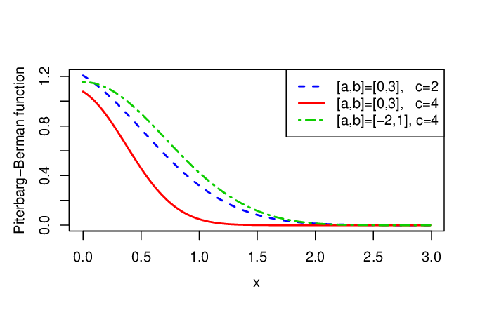
Figure 2. The Piterbarg-Berman function 𝒫​ℬ2h​(x,E)\mathcal{P\!B}_{2}^{h}(x,{E}) with h⁡(t)=c​|t|λ−t2h(t)=c\left\lvert t\right\rvert^{\lambda}-t^{2} for λ=2,c=1\lambda=2,c=1(left) and λ=2,c=2,4\lambda=2,c=2,4 (right).

In Figure 2 (and thereafter), we consider finite time interval E=[a,b]E=[a,b] and h⁡(t)=c​|t|λ−t2,c>0h(t)=c|t|^{\lambda}-t^{2},\,c>0 as in Proposition 2.1. Here we take λ=2,E=[0,3],[−2,1],[1,3],[−1,1],[0,4]\lambda=2,E=[0,3],[-2,1],[1,3],[-1,1],[0,4] and c=1,2,4c=1,2,4. We see that 𝒫​ℬ2h​(x,E),x∈[0,b−a]\mathcal{P\!B}_{2}^{h}(x,E),x\in[0,b-a] is decreasing slowly.

Refer to caption
Refer to caption
Figure 3. The Piterbarg-Berman function 𝒫​ℬ2h​(x,E)\mathcal{P\!B}_{2}^{h}(x,{E}) with drift function h⁡(t)=c​|t|−t2h(t)=c\left\lvert t\right\rvert-t^{2}.

In Figure 3, we draw 𝒫​ℬ2h​(x,E),E=[a,b]\mathcal{P\!B}_{2}^{h}(x,E),E=[a,b] with h⁡(t)=c​|t|−t2h(t)=c|t|-t^{2}. It seems more sensitive to the time interval EE of the same length and decreases strongly as x→0x\to 0 but indifferent for larger xx.

Refer to caption
(i) [a,b]=[1,5][a,b]=[1,5]
Refer to caption
(ii) [a,b]=[−1,2][a,b]=[-1,2]
Refer to caption
(iii) [a,b]=[1,4][a,b]=[1,4]
Refer to caption
(iv) [a,b]=[−1,1][a,b]=[-1,1]
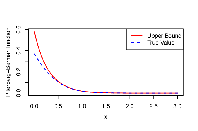
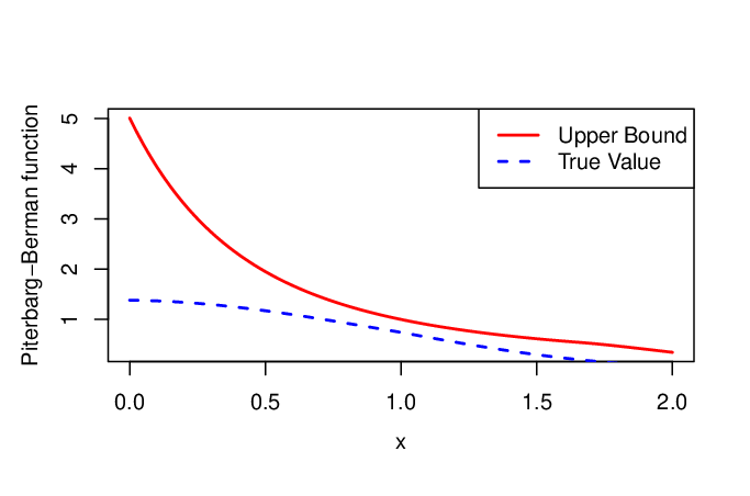
Figure 4. Upper bounds and true values of 𝒫​ℬ2h​(x,E)\mathcal{P\!B}_{2}^{h}(x,{E}) for drift function h⁡(t)=c​|t|λ−t2h(t)=c|t|^{\lambda}-t^{2} with λ=2,c=1\lambda=2,c=1 (top) and λ=2,c=2\lambda=2,c=2 (bottom).

In Figure 4, we apply Proposition 2.3 and show the efficiency of the upper bounds of 𝒫​ℬ2h​(x,E),E=[a,b]\mathcal{P\!B}_{2}^{h}(x,E),E=[a,b] with h⁡(t)=(c−1)​t2h(t)=(c-1)t^{2} for c=1,2c=1,2. Clearly, the upper bound of the Piterbarg-Berman function become closer to the true values for larger xx. The error is also determined by the time intervals and the coefficient cc of the drift function as well.

Overall, the Piterbarg-Berman function has nice properties with respect to the argument xx and the coefficient cc arising in the simple drift function h⁡(t)=c​|t|λ−t2h(t)=c|t|^{\lambda}-t^{2}. Meanwhile, its essential complexity is closely related to the observed time interval E=[a,b]{E=}[a,b] as well as the power index λ\lambda involved.

4. Proofs

Throughout the proofs, we keep the same notation aforementioned unless stated otherwise. We shall present the proofs of Theorem 1.1 and Propositions 2.1-2.3 one by one.

4.1. Proofs of Theorem 1.1 for 𝒫​ℬαh​(x)\mathcal{P\!B}_{\alpha}^{h}(x) with h⁡(t)=c​tα,c>0h(t)=ct^{\alpha},c>0 and α=1,2\alpha=1,2


Proof of (i) α=1\alpha=1. Recalling the sojourn time YzY_{z} given by (1.5), we have

(4.1) 𝒫ℬ1h(x)=(∫0∞+∫−∞0)ezℙ{Yz>x}dz=:I1(x)+I2(x).\displaystyle\mathcal{P\!B}_{1}^{h}(x)=\left(\int_{0}^{\infty}+\int_{-\infty}^{0}\right)e^{z}\mathbb{P}\left\{Y_{z}>x\right\}\text{\rm d}z=:I_{1}(x)+I_{2}(x).

We deal with the integrals I1​(x)I_{1}(x) and I2​(x)I_{2}(x) according to the upward and downward crossings.

For I1​(x)I_{1}(x). By the lack of upward jumps and the strong Markov property, we have for z≥0z\geq 0

ℙ{Yz>x}=ℙ{Y0>x}ℙ{supt≥0(2B1(t)−(1+c)t)≥z},\displaystyle\mathbb{P}\left\{Y_{z}>x\right\}=\mathbb{P}\left\{Y_{0}>x\right\}\mathbb{P}\left\{\sup_{t\geq 0}(\sqrt{2}B_{1}(t)-(1+c)t)\geq z\right\},

where, it follows from [29] that (see e.g., Eq. (3) in p. 255 therein)

ℙ{supt≥0(2B1(t)−(1+c)t)≥z}=e−(1+c)​z,z≥0,\displaystyle\mathbb{P}\left\{\sup_{t\geq 0}(\sqrt{2}B_{1}(t)-(1+c)t)\geq z\right\}=e^{-(1+c)z},\quad z\geq 0,
ℙ{Y0>x}=2(1+(1+c)2​x2)Ψ((1+c)x2)−(1+c)2​xφ((1+c)x/2)\displaystyle\mathbb{P}\left\{Y_{0}>x\right\}=2\left(1+\frac{(1+c)^{2}x}{2}\right)\Psi\left((1+c)\sqrt{\frac{x}{2}}\right)-(1+c)\sqrt{2x}\varphi\left((1+c)\sqrt{x/2}\right)
(4.2) =2​(1+xc2)​Ψ​(xc)−2​xc​φ​(xc),xc=(1+c)​x/2.\displaystyle\qquad\qquad\quad=2(1+x_{c}^{2})\Psi(x_{c})-2x_{c}\varphi(x_{c}),\quad x_{c}=(1+c)\sqrt{x/2}.

Therefore,

(4.3) I1(x)=∫0∞e−c​zdzℙ{Y0>x}=2c[(1+xc2)Ψ(xc)−xcφ(xc)].\displaystyle I_{1}(x)=\int_{0}^{\infty}e^{-cz}\text{\rm d}z\mathbb{P}\left\{Y_{0}>x\right\}=\frac{2}{c}\left[(1+x_{c}^{2})\Psi(x_{c})-x_{c}\varphi(x_{c})\right].

For I2​(x)I_{2}(x). Note that τz=inf{t≥0:2​B1​(t)−(1+c)​t≥z}\tau_{z}=\inf\{t\geq 0:\sqrt{2}B_{1}(t)-(1+c)t\geq z\} for given z<0z<0 is a stopping time with cumulative distribution function (cdf) and probability density function (pdf) given by

(4.4) ℙ{τz≤t}=Ψ(−z2​t−tc)+e−(1+c)​zΨ(−z2​t+tc),z<0,fz​(t)=−z2​t3​φ​(−z2​t−tc),tc=(1+c)​x/2,t>0\displaystyle\begin{split}\mathbb{P}\left\{\tau_{z}\leq t\right\}&=\Psi\left(\frac{-z}{\sqrt{2t}}-t_{c}\right)+e^{-(1+c)z}\Psi\left(\frac{-z}{\sqrt{2t}}+t_{c}\right),\quad z<0,\\ f_{z}(t)&=\frac{-z}{\sqrt{2t^{3}}}\varphi\left(\frac{-z}{\sqrt{2t}}-t_{c}\right),\quad t_{c}=(1+c)\sqrt{x/2},\,\,t>0\end{split}

by Eq. (3) in page 261 of [29] and the fact that φ⁡(z/2​t+tc)=e(1+c)​z​φ​(z/2​t−tc)\varphi(z/\sqrt{2t}+t_{c})=e^{(1+c)z}\varphi(z/\sqrt{2t}-t_{c}). Therefore, again by the strong Markov property, we have

ℙ{Yz>x}\displaystyle\mathbb{P}\left\{Y_{z}>x\right\} =ℙ{τz+∫τz∞𝕀(2B1(t)−(1+c)t>z)dt>x}\displaystyle=\mathbb{P}\left\{\tau_{z}+\int_{\tau_{z}}^{\infty}\mathbb{I}(\sqrt{2}B_{1}(t)-(1+c)t>z)\text{\rm d}t>x\right\}
=ℙ{τz+∫0∞𝕀(2[B1(t+τz)−B1(τz)]−(1+c)t>0)dt>x}\displaystyle=\mathbb{P}\left\{\tau_{z}+\int_{0}^{\infty}\mathbb{I}(\sqrt{2}[B_{1}(t+\tau_{z})-B_{1}(\tau_{z})]-(1+c)t>0)\text{\rm d}t>x\right\}
=ℙ{τz>x}+∫0xℙ{Y0>x−t}fz(t)dt,\displaystyle=\mathbb{P}\left\{\tau_{z}>x\right\}+\int_{0}^{x}\mathbb{P}\left\{Y_{0}>x-t\right\}f_{z}(t)\text{\rm d}t,

where the last step follows since τz\tau_{z} and Y0Y_{0} are independent. Consequently,

I2​(x)\displaystyle I_{2}(x) =∫0∞e−z[ℙ{τ−z>x}+∫0xℙ{Y0>x−t}f−z(t)dt]dz\displaystyle=\int_{0}^{\infty}e^{-z}\left[\mathbb{P}\left\{\tau_{-z}>x\right\}+\int_{0}^{x}\mathbb{P}\left\{Y_{0}>x-t\right\}f_{-z}(t)\text{\rm d}t\right]\text{\rm d}z
(4.5) =:I21​(x)+I22​(x).\displaystyle=:I_{21}(x)+I_{22}(x).

In the following, we deal with I21​(x)I_{21}(x) and I22​(x)I_{22}(x) subsequently. First, we have by (4.4)

I21​(x)\displaystyle I_{21}(x) =1−∫0∞e−z​[Ψ⁡(z2​x−xc)+e(1+c)​z​Ψ​(z2​x+xc)]​d​z\displaystyle=1-\int_{0}^{\infty}e^{-z}\left[\Psi\left(\frac{z}{\sqrt{2x}}-x_{c}\right)+e^{(1+c)z}\Psi\left(\frac{z}{\sqrt{2x}}+x_{c}\right)\right]\text{\rm d}z
(4.6) =1+cc​Ψ​(xc)−1−cc​Ψ​(xc′)​e−c​x,xc′=(1−c)​x/2.\displaystyle=\frac{1+c}{c}\Psi(x_{c})-\frac{1-c}{c}\Psi(x_{c}^{\prime})e^{-cx},\quad x_{c}^{\prime}=(1-c)\sqrt{x/2}.

Similarly, we have by (4.1), (4.4) and (4.1)

I22​(x)\displaystyle I_{22}(x) =∫0xℙ{Y0>x−t}[∫0∞e−zf−z(t)dz]dt\displaystyle=\int_{0}^{x}\mathbb{P}\left\{Y_{0}>x-t\right\}\Big[\int_{0}^{\infty}e^{-z}f_{-z}(t)\text{\rm d}z\Big]\text{\rm d}t
=2​∫0x{[(1+xc2)−tc2]​Ψ​(xc2−tc2)−xc2−tc2​φ​(xc2−tc2)}​[(1+c)​φ⁡(tc)tc−(1−c)​Ψ​(tc′)​e−c​t]​d​t\displaystyle=2\int_{0}^{x}\left\{[(1+x_{c}^{2})-t_{c}^{2}]\Psi(\sqrt{x_{c}^{2}-t_{c}^{2}})-\sqrt{x_{c}^{2}-t_{c}^{2}}\varphi(\sqrt{x_{c}^{2}-t_{c}^{2}})\right\}\Big[(1+c)\frac{\varphi(t_{c})}{t_{c}}-(1-c)\Psi(t_{c}^{\prime})e^{-ct}\Big]\text{\rm d}t
=:2{(1+c)[(1+xc2)A1−A2−A3]−|1−c|𝕀(c≠1)[(1+xc2)A4−A5−A6]\displaystyle=:2\Big\{(1+c)\big[(1+x_{c}^{2})A_{1}-A_{2}-A_{3}\big]-|1-c|\mathbb{I}\left(c\neq 1\right)\big[(1+x_{c}^{2})A_{4}-A_{5}-A_{6}\big]
+|1−c|𝕀(c>1)[(1+xc2)A4+−A5+−A6+]},\displaystyle\quad+|1-c|\mathbb{I}\left(c>1\right)\big[(1+x_{c}^{2})A_{4}^{+}-A_{5}^{+}-A_{6}^{+}\big]\Big\},

where, with tc=(1+c)​t/2,tc′=(1−c)​t/2t_{c}=(1+c)\sqrt{t/2},t_{c}^{\prime}=(1-c)\sqrt{t/2},

A1\displaystyle A_{1} =∫0xφ⁡(tc)tc​Ψ​(xc2−tc2)​d​t,A2=∫0xtc​φ​(tc)​Ψ​(xc2−tc2)​d​t,A3=e−xc2/22​π​∫0xxt−1​d​t,\displaystyle=\int_{0}^{x}\frac{\varphi(t_{c})}{t_{c}}\Psi(\sqrt{x_{c}^{2}-t_{c}^{2}})\text{\rm d}t,\quad A_{2}=\int_{0}^{x}t_{c}{\varphi(t_{c})}\Psi(\sqrt{x_{c}^{2}-t_{c}^{2}})\text{\rm d}t,\quad A_{3}=\frac{e^{-x_{c}^{2}/2}}{2\pi}\int_{0}^{x}\sqrt{\frac{x}{t}-1}\text{\rm d}t,
A4\displaystyle A_{4} =∫0xΨ⁡(xc2−tc2)​Ψ​(|tc′|)​e−c​t​d​t,A4+=∫0xΨ⁡(xc2−tc2)​e−c​t​d​t,\displaystyle=\int_{0}^{x}\Psi(\sqrt{x_{c}^{2}-t_{c}^{2}})\Psi(|t_{c}^{\prime}|)e^{-ct}\text{\rm d}t,\qquad\qquad\qquad A_{4}^{+}=\int_{0}^{x}\Psi(\sqrt{x_{c}^{2}-t_{c}^{2}})e^{-ct}\text{\rm d}t,
A5\displaystyle A_{5} =∫0xtc2​Ψ​(xc2−tc2)​Ψ​(|tc′|)​e−c​t​d​t,A5+=∫0xtc2​Ψ​(xc2−tc2)​e−c​t​d​t,\displaystyle=\int_{0}^{x}t_{c}^{2}\Psi(\sqrt{x_{c}^{2}-t_{c}^{2}})\Psi(|t_{c}^{\prime}|)e^{-ct}\text{\rm d}t,\quad\qquad\qquad A_{5}^{+}=\int_{0}^{x}t_{c}^{2}\Psi(\sqrt{x_{c}^{2}-t_{c}^{2}})e^{-ct}\text{\rm d}t,
A6\displaystyle A_{6} =∫0xxc2−tc2​φ​(xc2−tc2)​Ψ​(|tc′|)​e−c​t​d​t,A6+=∫0xxc2−tc2​φ​(xc2−tc2)​e−c​t​d​t.\displaystyle=\int_{0}^{x}\sqrt{x_{c}^{2}-t_{c}^{2}}\varphi(\sqrt{x_{c}^{2}-t_{c}^{2}})\Psi(|t_{c}^{\prime}|)e^{-ct}\text{\rm d}t,\qquad A_{6}^{+}=\int_{0}^{x}\sqrt{x_{c}^{2}-t_{c}^{2}}\varphi(\sqrt{x_{c}^{2}-t_{c}^{2}})e^{-ct}\text{\rm d}t.

Here the three terms A4+∼A6+A_{4}^{+}\sim A_{6}^{+} for c>1c>1 arises since Ψ⁡(tc′)=1−Ψ⁡(|tc′|)\Psi(t_{c}^{\prime})=1-\Psi(|t_{c}^{\prime}|) as tc′<0t_{c}^{\prime}<0, i.e., c>1c>1.

Next, we deal with I22​(x)I_{22}(x) by specifying the three sets of integrals: (i) A1∼A3A_{1}\sim A_{3} with c>0c>0; (ii) A4∼A6A_{4}\sim A_{6} with c≠1c\neq 1 and (iii) A4+∼A6+A_{4}^{+}\sim A_{6}^{+} with c>1c>1.

(ii) For A1∼A3A_{1}\sim A_{3} with c>0c>0. By the symmetry of standard normal distributions, we have

(1+c)2​A1\displaystyle(1+c)^{2}A_{1} =4​∫0xcφ⁡(v)​Ψ​(xc2−v2)​d​v\displaystyle=4\int_{0}^{x_{c}}\varphi(v)\Psi(\sqrt{x_{c}^{2}-v^{2}})\text{\rm d}v
(4.7) =(∫u2+v2>xc2−∫v2>xc2)φ(u)φ(v)dudv=e−xc2/2−2Ψ(xc),\displaystyle=\left(\int_{u^{2}+v^{2}>x_{c}^{2}}-\int_{v^{2}>x_{c}^{2}}\right)\varphi(u)\varphi(v)\text{\rm d}u\text{\rm d}v=e^{-x_{c}^{2}/2}-2\Psi(x_{c}),
(1+c)2​A2\displaystyle(1+c)^{2}A_{2} =4∫u2+v2>xc2,|v|<xcv2φ(v)φ(u)dudv=[∫u2+v2>xc2−∫|v|>xc]v2φ(v)φ(u)dudv\displaystyle=4\int_{u^{2}+v^{2}>x_{c}^{2},|v|<x_{c}}v^{2}\varphi(v)\varphi(u)\text{\rm d}u\text{\rm d}v=\left[\int_{u^{2}+v^{2}>x_{c}^{2}}-\int_{|v|>x_{c}}\right]v^{2}\varphi(v)\varphi(u)\text{\rm d}u\text{\rm d}v
=12​∫u2+v2>xc2(u2+v2)​φ​(u)​φ​(v)​d​u​d​v−2​[Φ⁡(v)−v​φ​(v)]|xc∞\displaystyle=\frac{1}{2}\int_{u^{2}+v^{2}>x_{c}^{2}}(u^{2}+v^{2})\varphi(u)\varphi(v)\text{\rm d}u\text{\rm d}v-2[\Phi(v)-v\varphi(v)]|_{x_{c}}^{\infty}
=−(1+t)​e−t|xc2/2∞−2​[Φ⁡(v)−v​φ​(v)]|xc∞\displaystyle=-(1+t)e^{-t}|_{x_{c}^{2}/2}^{\infty}-2[\Phi(v)-v\varphi(v)]|_{x_{c}}^{\infty}
(4.8) =[1+xc2/2]e−xc2/2−2[Ψ(xc)+xcφ(xc)]=:(−2)m(xc).\displaystyle=[1+x_{c}^{2}/2]e^{-x_{c}^{2}/2}-2[\Psi(x_{c})+x_{c}\varphi(x_{c})]=:(-2)\mathrm{m}(x_{c}).

For A3A_{3}, we take s=t/x,0<t<xs=\sqrt{t/x},0<t<x and thus

A3=xπe−xc2/2∫011−s2dt=xe−xc2/24.\displaystyle A_{3}=\frac{x}{\pi}e^{-x_{c}^{2}/2}\int_{0}^{1}\sqrt{1-s^{2}}\text{\rm d}t=\frac{xe^{-x_{c}^{2}/2}}{4}.

It follows then that

I22(1)​(x)2​(1+c)\displaystyle\frac{I_{22}^{(1)}(x)}{2(1+c)} :=(1+xc2)A1−A2−A3=1+xc2(1+c)2[e−xc2/2−2Ψ(xc)]\displaystyle:=(1+x_{c}^{2})A_{1}-A_{2}-A_{3}=\frac{1+x_{c}^{2}}{(1+c)^{2}}\left[e^{-x_{c}^{2}/2}-2\Psi(x_{c})\right]
−[1+xc2/2]e−xc2/2−2[Ψ(xc)+xcφ(xc)](1+c)2−x4e−xc2/2\displaystyle\quad-\frac{[1+x_{c}^{2}/2]e^{-x_{c}^{2}/2}-2[\Psi(x_{c})+x_{c}\varphi(x_{c})]}{(1+c)^{2}}-\frac{x}{4}e^{-x_{c}^{2}/2}
=2(1+c)2​[xc​φ​(xc)−xc2​Ψ​(xc)].\displaystyle=\frac{2}{(1+c)^{2}}\left[x_{c}\varphi(x_{c})-x_{c}^{2}\Psi(x_{c})\right].

(ii) For A4∼A6A_{4}\sim A_{6} with c≠1c\neq 1. We rewrite first A4A_{4} and A5A_{5} as follows.

c​A4\displaystyle cA_{4} =∫0xΨ⁡(xc2−tc2)​Ψ​(|tc′|)​e−c​t​d​c​t\displaystyle=\int_{0}^{x}\Psi(\sqrt{x_{c}^{2}-t_{c}^{2}})\Psi(|t_{c}^{\prime}|)e^{-ct}\text{\rm d}ct
=∫0c​x∫xc​1−t/(c​x)∞∫|xc′|​t/(c​x)∞e−t​φ​(u)​φ​(v)​d​t​d​u​d​v\displaystyle=\int_{0}^{cx}\int_{x_{c}\sqrt{1-t/(cx)}}^{\infty}\int_{|x_{c}^{\prime}|\sqrt{t/(cx)}}^{\infty}e^{-t}\varphi(u)\varphi(v)\text{\rm d}t\text{\rm d}u\text{\rm d}v
=xc​|xc′|​∫0∞∫0∞φ⁡(xc​u)​φ​(|xc′|​v)​∫c​x​max⁡(0,1−u2)c​x​min⁡(1,v2)d​[−e−t]​d​u​d​v,\displaystyle=x_{c}|x_{c}^{\prime}|\int_{0}^{\infty}\int_{0}^{\infty}\varphi(x_{c}u)\varphi(|x_{c}^{\prime}|v)\int_{cx\max(0,1-u^{2})}^{cx\min(1,v^{2})}\text{\rm d}[-e^{-t}]\text{\rm d}u\text{\rm d}v,
c2​x​A5\displaystyle c^{2}xA_{5} =xc2​∫0x(c​t)​Ψ​(xc2−tc2)​Ψ​(|tc′|)​e−c​t​d​(c​t)\displaystyle=x_{c}^{2}\int_{0}^{x}(ct)\Psi(\sqrt{x_{c}^{2}-t_{c}^{2}})\Psi(|t_{c}^{\prime}|)e^{-ct}\text{\rm d}(ct)
=xc3​|xc′|​∫0∞∫0∞φ⁡(xc​u)​φ​(|xc′|​v)​∫c​x​max⁡(0,1−u2)c​x​min⁡(1,v2)d​[−(1+t)​e−t]​d​u​d​v\displaystyle=x_{c}^{3}|x_{c}^{\prime}|\int_{0}^{\infty}\int_{0}^{\infty}\varphi(x_{c}u)\varphi(|x_{c}^{\prime}|v)\int_{cx\max(0,1-u^{2})}^{cx\min(1,v^{2})}\text{\rm d}[-(1+t)e^{-t}]\text{\rm d}u\text{\rm d}v
=c​xc2​A4+xc3​|xc′|​∫0∞∫0∞φ⁡(xc​u)​φ​(|xc′|​v)​∫c​x​max⁡(0,1−u2)c​x​min⁡(1,v2)d​[−t​e−t]​d​u​d​v\displaystyle=cx_{c}^{2}A_{4}+x_{c}^{3}|x_{c}^{\prime}|\int_{0}^{\infty}\int_{0}^{\infty}\varphi(x_{c}u)\varphi(|x_{c}^{\prime}|v)\int_{cx\max(0,1-u^{2})}^{cx\min(1,v^{2})}\text{\rm d}[-te^{-t}]\text{\rm d}u\text{\rm d}v
=:c​xc2​A4+B4.\displaystyle=:cx_{c}^{2}A_{4}+B_{4}.

We decompose further the integrals A4A_{4} and B4B_{4} by specifying the integral limits as below

c​A4\displaystyle cA_{4} =xc|xc′|(∫01∫01∫c​x​(1−u2)c​x​v2+∫01∫1∞∫c​x​(1−u2)c​x\displaystyle=x_{c}|x_{c}^{\prime}|\left(\int_{0}^{1}\int_{0}^{1}\int_{cx(1-u^{2})}^{cxv^{2}}+\int_{0}^{1}\int_{1}^{\infty}\int_{cx(1-u^{2})}^{cx}\right.
+∫1∞∫01∫0c​x​v2+∫1∞∫1∞∫0c​x)φ(xcu)φ(|xc′|v)d[−e−t]dudv\displaystyle\quad+\left.\int_{1}^{\infty}\int_{0}^{1}\int_{0}^{cxv^{2}}+\int_{1}^{\infty}\int_{1}^{\infty}\int_{0}^{cx}\right)\varphi(x_{c}u)\varphi(|x_{c}^{\prime}|v)\text{\rm d}[-e^{-t}]\text{\rm d}u\text{\rm d}v
=:I1+I2+I3+I4,\displaystyle=:I_{1}+I_{2}+I_{3}+I_{4},
B4\displaystyle B_{4} =xc3|xc′|(∫01∫01∫c​x​(1−u2)c​x​v2+∫01∫1∞∫c​x​(1−u2)c​x\displaystyle=x_{c}^{3}|x_{c}^{\prime}|\left(\int_{0}^{1}\int_{0}^{1}\int_{cx(1-u^{2})}^{cxv^{2}}+\int_{0}^{1}\int_{1}^{\infty}\int_{cx(1-u^{2})}^{cx}\right.
+∫1∞∫01∫0c​x​v2+∫1∞∫1∞∫0c​x)φ(xcu)φ(|xc′|v)d[−te−t]dudv\displaystyle\quad+\left.\int_{1}^{\infty}\int_{0}^{1}\int_{0}^{cxv^{2}}+\int_{1}^{\infty}\int_{1}^{\infty}\int_{0}^{cx}\right)\varphi(x_{c}u)\varphi(|x_{c}^{\prime}|v)\text{\rm d}[-te^{-t}]\text{\rm d}u\text{\rm d}v
=:J1+J2+J3+J4.\displaystyle=:J_{1}+J_{2}+J_{3}+J_{4}.

We deal first with I3,I4I_{3},I_{4} and J3,J4J_{3},J_{4}. Since φ⁡(|xc|​u)​ec​x​u2=φ⁡(|xc′|​u),φ⁡(|xc′|​v)​ec​x​v2=φ⁡(|xc|​v)\varphi(|x_{c}|u)e^{cxu^{2}}=\varphi(|x_{c}^{\prime}|u),\varphi(|x_{c}^{\prime}|v)e^{cxv^{2}}=\varphi(|x_{c}|v), we have

I3\displaystyle I_{3} =Ψ⁡(xc)​∫01|xc′|​[φ⁡(|xc′|​v)−φ⁡(xc​v)]​d​v\displaystyle={\Psi(x_{c})}\int_{0}^{1}|x_{c}^{\prime}|\left[\varphi(|x_{c}^{\prime}|v)-\varphi(x_{c}v)\right]\text{\rm d}v
=Ψ⁡(xc)​[[0.5−Ψ⁡(|xc′|)]−|1−c|1+c​[0.5−Ψ⁡(xc)]]\displaystyle={\Psi(x_{c})}\left[[0.5-\Psi(|x_{c}^{\prime}|)]-\frac{|1-c|}{1+c}[0.5-\Psi(x_{c})]\right]
J3\displaystyle J_{3} =−c​x​Ψ​(xc)​xc2|xc′|∫01v2​φ​(xc​v)​d​v=−|1−c|1+c​(c​x)​Ψ​(xc)​ω​(xc)\displaystyle=-cx{\Psi(x_{c})}x_{c}^{2}|x_{c}^{\prime}|\int_{0}^{1}v^{2}\varphi(x_{c}v)\text{\rm d}v=-\frac{|1-c|}{1+c}(cx){\Psi(x_{c})}\omega(x_{c})

and

I4=Ψ⁡(xc)​Ψ​(|xc′|)​[1−e−c​x],J4=−(c​x)​e−c​x​xc2​Ψ​(xc)​Ψ​(|xc′|).\displaystyle I_{4}=\Psi(x_{c})\Psi(|x_{c}^{\prime}|)[1-e^{-cx}],\quad J_{4}=-(cx)e^{-cx}x_{c}^{2}\Psi(x_{c})\Psi(|x_{c}^{\prime}|).

For I1,I2I_{1},I_{2} and J1,J2J_{1},J_{2}, we have

I1\displaystyle I_{1} =xc​|xc′|​∫0<u,v<1,u2+v2>1[e−c​x​φ​(|xc′|​u)​φ​(|xc′|​v)−φ⁡(xc​u)​φ​(xc​v)]​d​u​d​v\displaystyle=x_{c}|x_{c}^{\prime}|\int_{0<u,v<1,u^{2}+v^{2}>1}\left[e^{-cx}\varphi(|x_{c}^{\prime}|u)\varphi(|x_{c}^{\prime}|v)-\varphi(x_{c}u)\varphi(x_{c}v)\right]\text{\rm d}u\text{\rm d}v
=1+c|1−c|​e−c​x​μ​(|xc′|)−|1−c|1+c​μ​(xc),\displaystyle=\frac{1+c}{|1-c|}e^{-cx}\mu(|x_{c}^{\prime}|)-\frac{|1-c|}{1+c}\mu(x_{c}),
J1\displaystyle J_{1} =c​x​xc3​|xc′|​∫0<u,v<1,u2+v2>1[e−c​x​(1−u2)​φ​(|xc′|​u)​φ​(|xc′|​v)−v2​φ​(xc​u)​φ​(xc​v)]​d​u​d​v\displaystyle=cxx_{c}^{3}|x_{c}^{\prime}|\int_{0<u,v<1,u^{2}+v^{2}>1}\Big[e^{-cx}(1-u^{2})\varphi(|x_{c}^{\prime}|u)\varphi(|x_{c}^{\prime}|v)-v^{2}\varphi(x_{c}u)\varphi(x_{c}v)\Big]\text{\rm d}u\text{\rm d}v
=c​x​{1+c|1−c|​xc2​e−c​x​μ​(|xc′|)−(1+c)3|1−c|3​e−c​x​ν​(|xc′|)−|1−c|1+c​ν​(xc)},\displaystyle=cx\left\{\frac{1+c}{|1-c|}x_{c}^{2}e^{-cx}\mu(|x_{c}^{\prime}|)-\frac{(1+c)^{3}}{|1-c|^{3}}e^{-cx}\nu(|x_{c}^{\prime}|)-\frac{|1-c|}{1+c}\nu(x_{c})\right\},

where μ⁡(a)\mu(a) and ν⁡(a)\nu(a) are given by

μ⁡(a):=a2​∫0<u,v<1,u2+v2>1φ⁡(a​u)​φ​(a​v)​d​u​d​v=Φ⁡(a)−0.5−a​φ​(a),ν⁡(a):=a4​∫0<u,v<1,u2+v2>1u2​φ​(a​u)​φ​(a​v)​d​u​d​v=[Φ⁡(a)−0.5]​ω​(a)+(1+a2/2)e−a2/2−14.\displaystyle\begin{split}\mu(a)&:=a^{2}\int_{0<u,v<1,u^{2}+v^{2}>1}\varphi(au)\varphi(av)\text{\rm d}u\text{\rm d}v=\Phi(a)-0.5-a\varphi(a),\\ \nu(a)&:=a^{4}\int_{0<u,v<1,u^{2}+v^{2}>1}u^{2}\varphi(au)\varphi(av)\text{\rm d}u\text{\rm d}v=[\Phi(a)-0.5]\omega(a)+\frac{(1+a^{2}/2)e^{-a^{2}/2}-1}{4}.\end{split}

Now, for I2I_{2} and J2J_{2}, we have

I2\displaystyle I_{2} =Ψ⁡(|xc′|)​e−c​x​∫01xc​[φ⁡(|xc′|​u)−φ⁡(xc​u)]​d​u\displaystyle=\Psi(|x_{c}^{\prime}|)e^{-cx}\int_{0}^{1}x_{c}\left[\varphi(|x_{c}^{\prime}|u)-\varphi(x_{c}u)\right]\text{\rm d}u
=Ψ⁡(|xc′|)​e−c​x​[1+c|1−c|​[0.5−Ψ⁡(|xc′|)]−[0.5−Ψ⁡(xc)]],\displaystyle=\Psi(|x_{c}^{\prime}|)e^{-cx}\left[\frac{1+c}{|1-c|}[0.5-\Psi(|x_{c}^{\prime}|)]-[0.5-\Psi(x_{c})]\right],
J2\displaystyle J_{2} =c​x​e−c​x​Ψ​(|xc′|)​∫01xc3​[(1−u2)​φ​(|xc′|​u)−φ⁡(xc​u)]​d​u\displaystyle=cxe^{-cx}\Psi(|x_{c}^{\prime}|)\int_{0}^{1}x_{c}^{3}\left[(1-u^{2})\varphi(|x_{c}^{\prime}|u)-\varphi(x_{c}u)\right]\text{\rm d}u
=c​x​e−c​x​Ψ​(|xc′|)​{1+c|1−c|​xc2​[Φ⁡(|xc′|)−0.5]−(1+c)3|1−c|3​ω​(|xc′|)−xc2​[Φ⁡(xc)−0.5]}.\displaystyle=cxe^{-cx}\Psi(|x_{c}^{\prime}|)\left\{\frac{1+c}{|1-c|}x_{c}^{2}[\Phi(|x_{c}^{\prime}|)-0.5]-\frac{(1+c)^{3}}{|1-c|^{3}}\omega(|x_{c}^{\prime}|)-x_{c}^{2}[\Phi(x_{c})-0.5]\right\}.

Therefore, summing up I1∼I4I_{1}\sim I_{4} and J1∼J4J_{1}\sim J_{4} to give A4A_{4} and B4B_{4} by putting μ⁡(⋅),ν⁡(⋅),ω⁡(⋅)\mu(\cdot),\nu(\cdot),\omega(\cdot) together with the fact that ν⁡(a)=−0.5​m​(a)−Ψ⁡(a)​ω​(a)\nu(a)=-0.5\mathrm{m}(a)-\Psi(a)\omega(a) for m⁡(⋅)\mathrm{m}(\cdot) given by (4.1), we have

c​A4\displaystyle cA_{4} =I1+I2+I3+I4\displaystyle=I_{1}+I_{2}+I_{3}+I_{4}
=c|1−c2|e−xc2/2+|1−c|1+cΦ(xc)Ψ(xc)−(1+c)​e−c​x|1−c|Φ(|xc′|)Ψ(|xc′|)\displaystyle=\frac{c}{|1-c^{2}|}e^{-x_{c}^{2}/2}+\frac{|1-c|}{1+c}\Phi(x_{c})\Psi(x_{c})-\frac{(1+c)e^{-cx}}{|1-c|}\Phi(|x_{c}^{\prime}|)\Psi(|x_{c}^{\prime}|)
+Ψ⁡(|xc′|)​e−c​x​[1+c|1−c|​[0.5−Ψ⁡(|xc′|)]−[0.5−Ψ⁡(xc)]]\displaystyle\quad+\Psi(|x_{c}^{\prime}|)e^{-cx}\left[\frac{1+c}{|1-c|}[0.5-\Psi(|x_{c}^{\prime}|)]-[0.5-\Psi(x_{c})]\right]
+Ψ⁡(xc)​[[0.5−Ψ⁡(|xc′|)]−|1−c|1+c​[0.5−Ψ⁡(xc)]]+Ψ⁡(xc)​Ψ​(|xc′|)​[1−e−c​x]\displaystyle\quad+{\Psi(x_{c})}\left[[0.5-\Psi(|x_{c}^{\prime}|)]-\frac{|1-c|}{1+c}[0.5-\Psi(x_{c})]\right]+\Psi(x_{c})\Psi(|x_{c}^{\prime}|)[1-e^{-cx}]
=max(1,c)[Ψ⁡(xc)1+c−Ψ⁡(|xc′|)|1−c|e−c​x]+c|1−c2|e−xc2/2,\displaystyle=\max(1,c)\left[\frac{\Psi(x_{c})}{1+c}-\frac{\Psi(|x_{c}^{\prime}|)}{|1-c|}e^{-cx}\right]+\frac{c}{|1-c^{2}|}e^{-x_{c}^{2}/2},
B4/[c​x]\displaystyle B_{4}/[cx] =(J1+J2+J3+J4)/(cx)=xc241+c|1−c|e−xc2/2−xc2max⁡(1,c)|1−c|e−c​xΨ(|xc′|)\displaystyle=(J_{1}+J_{2}+J_{3}+J_{4})/(cx)=\frac{x_{c}^{2}}{4}\frac{1+c}{|1-c|}e^{-x_{c}^{2}/2}-x_{c}^{2}\frac{\max(1,c)}{|1-c|}e^{-cx}\Psi(|x_{c}^{\prime}|)
+|1−c|2​(1+c)​(Ψ⁡(xc)+xc​φ​(xc)−(1+xc2/2)e−xc2/22)\displaystyle\quad+\frac{|1-c|}{2(1+c)}\left(\Psi(x_{c})+x_{c}\varphi(x_{c})-\frac{(1+x_{c}^{2}/2)e^{-x_{c}^{2}/2}}{2}\right)
+(1+c)32​|1−c|3​e−c​x​(Ψ⁡(|xc′|)+|xc′|​φ​(|xc′|)−(1+|xc′|2/2)e−|xc′|2/22)\displaystyle\quad+\frac{(1+c)^{3}}{2|1-c|^{3}}e^{-cx}\left(\Psi(|x_{c}^{\prime}|)+|x_{c}^{\prime}|\varphi(|x_{c}^{\prime}|)-\frac{(1+|x_{c}^{\prime}|^{2}/2)e^{-|x_{c}^{\prime}|^{2}/2}}{2}\right)
=xc241+c|1−c|e−xc2/2−xc2max⁡(1,c)|1−c|e−c​xΨ(|xc′|)+|1−c|2​(1+c)m(xc)+(1+c)32​|1−c|3e−c​xm(|xc′|).\displaystyle=\frac{x_{c}^{2}}{4}\frac{1+c}{|1-c|}e^{-x_{c}^{2}/2}-x_{c}^{2}\frac{\max(1,c)}{|1-c|}e^{-cx}\Psi(|x_{c}^{\prime}|)+\frac{|1-c|}{2(1+c)}\mathrm{m}(x_{c})+\frac{(1+c)^{3}}{2|1-c|^{3}}e^{-cx}\mathrm{m}(|x_{c}^{\prime}|).

Next, we turn to A6A_{6}. Since φ⁡(xc2−tc2)​ec⁡(x−t)=φ⁡(tc′)\varphi(\sqrt{x_{c}^{2}-t_{c}^{2}})e^{c(x-t)}=\varphi(t_{c}^{\prime}), we have by the integral of A2A_{2} given in (4.1)

A6\displaystyle A_{6} =1+c|1−c|​e−c​x​∫0x|tc′|​φ​(tc′)​Ψ​(|xc′|2−tc′2)​d​t\displaystyle=\frac{1+c}{|1-c|}e^{-cx}\int_{0}^{x}|t_{c}^{\prime}|\varphi(t_{c}^{\prime})\Psi\left(\sqrt{|x_{c}^{\prime}|^{2}-t_{c}^{\prime 2}}\right)\text{\rm d}t
=4​(1+c)|1−c|3​e−c​x​∫0|xc′|v2​φ​(v)​Ψ​(|xc′|2−v2)​d​v=−2​(1+c)|1−c|3​e−c​x​m​(|xc′|).\displaystyle=\frac{4(1+c)}{|1-c|^{3}}e^{-cx}\int_{0}^{|x_{c}^{\prime}|}v^{2}\varphi(v)\Psi\left(\sqrt{|x_{c}^{\prime}|^{2}-v^{2}}\right)\text{\rm d}v=-\frac{2(1+c)}{|1-c|^{3}}e^{-cx}\mathrm{m}(|x_{c}^{\prime}|).

Therefore, it follows by A5=xc2/(c​x)​A4+B4/(c2​x)A_{5}=x_{c}^{2}/(cx)A_{4}+B_{4}/(c^{2}x) that

I22(2)​(x)2​|1−c|\displaystyle\frac{I_{22}^{(2)}(x)}{2\left\lvert 1-c\right\rvert} :=(1+xc2)​A4−A5−A6=[1+xc2​(1−1c​x)]​A4−1c​B4c​x−A6\displaystyle:=(1+x_{c}^{2})A_{4}-A_{5}-A_{6}=\left[1+x_{c}^{2}\left(1-\frac{1}{cx}\right)\right]A_{4}-\frac{1}{c}\frac{B_{4}}{cx}-A_{6}
=[1+xc2(1−1c​x)]{max⁡(1,c)c[Ψ⁡(xc)1+c−Ψ⁡(|xc′|)|1−c|e−c​x]+1|1−c2|e−xc2/2}\displaystyle=\left[1+x_{c}^{2}\left(1-\frac{1}{cx}\right)\right]\left\{\frac{\max(1,c)}{c}\left[\frac{\Psi(x_{c})}{1+c}-\frac{\Psi(|x_{c}^{\prime}|)}{|1-c|}e^{-cx}\right]+\frac{1}{|1-c^{2}|}e^{-x_{c}^{2}/2}\right\}
−xc24​c1+c|1−c|e−xc2/2+xc2cmax⁡(1,c)|1−c|e−c​xΨ(|xc′|)−|1−c|2​c​(1+c)m(xc)−1+c2​c​|1−c|e−c​xm(|xc′|)\displaystyle\quad-\frac{x_{c}^{2}}{4c}\frac{1+c}{|1-c|}e^{-x_{c}^{2}/2}+\frac{x_{c}^{2}}{c}\frac{\max(1,c)}{|1-c|}e^{-cx}\Psi(|x_{c}^{\prime}|)-\frac{|1-c|}{2c(1+c)}\mathrm{m}(x_{c})-\frac{1+c}{2c|1-c|}e^{-cx}\mathrm{m}(|x_{c}^{\prime}|)
=[1+xc2(1−1c​x)]max⁡(1,c)cΨ⁡(xc)1+c−12​c​|1−c|[(1−c)22​(1+c)xc2+1+c21+c]e−xc2/2\displaystyle=\left[1+x_{c}^{2}\left(1-\frac{1}{cx}\right)\right]\frac{\max(1,c)}{c}\frac{\Psi(x_{c})}{1+c}-\frac{1}{2c|1-c|}\left[\frac{(1-c)^{2}}{2(1+c)}x_{c}^{2}+\frac{1+c^{2}}{1+c}\right]e^{-x_{c}^{2}/2}
(4.9) +1+c22​c2​max⁡(1,c)|1−c|​e−c​x​Ψ​(|xc′|)−|1−c|2​c​(1+c)​m​(xc)−1+c2​c​|1−c|​e−c​x​m​(|xc′|).\displaystyle\quad+\frac{1+c^{2}}{2c^{2}}\frac{\max(1,c)}{\left\lvert 1-c\right\rvert}e^{-cx}\Psi(|x_{c}^{\prime}|)-\frac{|1-c|}{2c(1+c)}\mathrm{m}(x_{c})-\frac{1+c}{2c|1-c|}e^{-cx}\mathrm{m}(|x_{c}^{\prime}|).

(iii) For A4+∼A6+A_{4}^{+}\sim A_{6}^{+} with c>1c>1. Following similar arguments of A4∼A6A_{4}\sim A_{6}, we have

c​A4+\displaystyle cA_{4}^{+} =xc​∫0∞φ⁡(xc​u)​∫c​x​max⁡(0,1−u2)c​xd​[−e−t]​d​u\displaystyle=x_{c}\int_{0}^{\infty}\varphi(x_{c}u)\int_{cx\max(0,1-u^{2})}^{cx}\text{\rm d}[-e^{-t}]\text{\rm d}u
=xc​e−c​x​∫01[φ⁡(xc′​u)−φ⁡(xc​u)]​d​u+(1−e−c​x)​Ψ​(xc)\displaystyle=x_{c}e^{-cx}\int_{0}^{1}\left[\varphi(x_{c}^{\prime}u)-\varphi(x_{c}u)\right]\text{\rm d}u+(1-e^{-cx})\Psi(x_{c})
=e−c​x|1−c|​[1−(1+c)​Ψ​(|xc′|)]+Ψ⁡(xc),\displaystyle=\frac{e^{-cx}}{\left\lvert 1-c\right\rvert}\big[1-(1+c)\Psi(|x_{c}^{\prime}|)\big]+\Psi(x_{c}),
c2​x​A5+\displaystyle c^{2}xA_{5}^{+} =xc3​∫0∞φ⁡(xc​u)​∫c​x​max⁡(0,1−u2)c​xd​[−(1+t)​e−t]​d​u=:c​xc2​A4++B4+,\displaystyle=x_{c}^{3}\int_{0}^{\infty}\varphi(x_{c}u)\int_{cx\max(0,1-u^{2})}^{cx}\text{\rm d}[-(1+t)e^{-t}]\text{\rm d}u=:cx_{c}^{2}A_{4}^{+}+B_{4}^{+},

with

B4+\displaystyle B_{4}^{+} =xc3​∫0∞φ⁡(xc​u)​∫c​x​max⁡(0,1−u2)c​xd​[−t​e−t]​d​u\displaystyle=x_{c}^{3}\int_{0}^{\infty}\varphi(x_{c}u)\int_{cx\max(0,1-u^{2})}^{cx}\text{\rm d}[-te^{-t}]\text{\rm d}u
=xc3(∫01∫c​x​(1−u2)c​x+∫1∞∫0c​x)d[−te−t]φ(xcu)du\displaystyle=x_{c}^{3}\left(\int_{0}^{1}\int_{cx(1-u^{2})}^{cx}+\int_{1}^{\infty}\int_{0}^{cx}\right)\text{\rm d}[-te^{-t}]\varphi(x_{c}u)\text{\rm d}u
=c​x​e−c​x​[∫01xc3​[(1−u2)​φ​(|xc′|​u)−φ⁡(xc​u)]​d​u−xc2​Ψ​(xc)]\displaystyle=cxe^{-cx}\Big[\int_{0}^{1}x_{c}^{3}[(1-u^{2})\varphi(|x_{c}^{\prime}|u)-\varphi(x_{c}u)]\text{\rm d}u-x_{c}^{2}\Psi(x_{c})\Big]
=c​x​e−c​x​[xc2|1−c|−1+c|1−c|​xc2​Ψ​(|xc′|)−(1+c)3|1−c|3​ω​(|xc′|)].\displaystyle=cxe^{-cx}\Big[\frac{x_{c}^{2}}{\left\lvert 1-c\right\rvert}-\frac{1+c}{\left\lvert 1-c\right\rvert}x_{c}^{2}\Psi(|x_{c}^{\prime}|)-\frac{(1+c)^{3}}{\left\lvert 1-c\right\rvert^{3}}\omega(|x_{c}^{\prime}|)\Big].

For A6+A_{6}^{+}, by a change of variable s=t−xs=t-x and ec​t​φ​(tc)=φ⁡(|tc′|)e^{ct}\varphi(t_{c})=\varphi(|t_{c}^{\prime}|)

A6+=1+c|1−c|​e−c​x​∫0x|tc′|​φ​(|tc′|)​d​t=4​(1+c)|1−c|3​e−c​x​∫0|xc′|s2​φ​(s)​d​t=4​(1+c)|1−c|3​e−c​x​ω​(|xc′|).\displaystyle A_{6}^{+}=\frac{1+c}{\left\lvert 1-c\right\rvert}e^{-cx}\int_{0}^{x}|t_{c}^{\prime}|\varphi(|t_{c}^{\prime}|)\text{\rm d}t=\frac{4(1+c)}{\left\lvert 1-c\right\rvert^{3}}e^{-cx}\int_{0}^{|x_{c}^{\prime}|}s^{2}\varphi(s)\text{\rm d}t=\frac{4(1+c)}{\left\lvert 1-c\right\rvert^{3}}e^{-cx}\omega(|x_{c}^{\prime}|).

Therefore, we have (recall that A5+=xc2/(c​x)​A4++B4+/(c2​x)A_{5}^{+}=x_{c}^{2}/(cx)A_{4}^{+}+B_{4}^{+}/(c^{2}x))

I22(3)​(x)2​|1−c|\displaystyle\frac{I_{22}^{(3)}(x)}{2\left\lvert 1-c\right\rvert} =[(1+xc2)​A4+−A5+−A6+]\displaystyle=[(1+x_{c}^{2})A_{4}^{+}-A_{5}^{+}-A_{6}^{+}]
=[1+xc2​(1−1c​x)]​A4+−1c2​x​B4+−A6+\displaystyle=\left[1+x_{c}^{2}\left(1-\frac{1}{cx}\right)\right]A_{4}^{+}-\frac{1}{c^{2}x}B_{4}^{+}-A_{6}^{+}
=[1+xc2​(1−1c​x)]​[e−c​xc​(1|1−c|−1+c|1−c|​Ψ​(|xc′|))+Ψ⁡(xc)c]\displaystyle=\left[1+x_{c}^{2}\left(1-\frac{1}{cx}\right)\right]\left[\frac{e^{-cx}}{c}\left(\frac{1}{\left\lvert 1-c\right\rvert}-\frac{1+c}{\left\lvert 1-c\right\rvert}\Psi(|x_{c}^{\prime}|)\right)+\frac{\Psi(x_{c})}{c}\right]
−e−c​xc​[xc2|1−c|−1+c|1−c|​xc2​Ψ​(|xc′|)−1+c|1−c|​ω​(|xc′|)]\displaystyle\quad-\frac{e^{-cx}}{c}\Big[\frac{x_{c}^{2}}{\left\lvert 1-c\right\rvert}-\frac{1+c}{\left\lvert 1-c\right\rvert}x_{c}^{2}\Psi(|x_{c}^{\prime}|)-\frac{1+c}{\left\lvert 1-c\right\rvert}\omega(|x_{c}^{\prime}|)\Big]
(4.10) =−1+c22​c​|1−c|​e−c​xc​[1−(1+c)​Ψ​(|xc′|)]+[1+xc2​(1−1c​x)]​Ψ⁡(xc)c+e−c​xc​1+c|1−c|​ω​(|xc′|).\displaystyle=-\frac{1+c^{2}}{2c|1-c|}\frac{e^{-cx}}{c}\big[1-(1+c)\Psi(|x_{c}^{\prime}|)\big]+\left[1+x_{c}^{2}\left(1-\frac{1}{cx}\right)\right]\frac{\Psi(x_{c})}{c}+\frac{e^{-cx}}{c}\frac{1+c}{\left\lvert 1-c\right\rvert}\omega(|x_{c}^{\prime}|).

Consequently, the desired expression of 𝒫​ℬαh​(x){\mathcal{P\!B}}_{\alpha}^{h}(x) follows by (4.3), (4.1) and (4.1). Indeed,

c⁡[I1​(x)+I21​(x)+I22(1)​(x)]\displaystyle c[I_{1}(x)+I_{21}(x)+I_{22}^{(1)}(x)] =2​[(1+xc2)​Ψ​(xc)−xc​φ​(xc)]\displaystyle=2\left[(1+x_{c}^{2})\Psi(x_{c})-x_{c}\varphi(x_{c})\right]
+[(1+c)​Ψ​(xc)−(1−c)​Ψ​(xc′)​e−c​x]+4​c1+c​[xc​φ​(xc)−xc2​Ψ​(xc)]\displaystyle\quad+\left[(1+c)\Psi(x_{c})-(1-c)\Psi(x_{c}^{\prime})e^{-cx}\right]+\frac{4c}{1+c}\left[x_{c}\varphi(x_{c})-x_{c}^{2}\Psi(x_{c})\right]
(4.11) =[3+c+(1−c2)​x]​Ψ​(xc)−2​(1−c)1+c​xc​φ​(xc)−(1−c)​Ψ​(xc′)​e−c​x,\displaystyle=[3+c+(1-c^{2})x]\Psi(x_{c})-\frac{2(1-c)}{1+c}x_{c}\varphi(x_{c})-(1-c)\Psi(x_{c}^{\prime})e^{-cx},

which together with (4.1) implies that

c⁡[I1​(x)+I21​(x)+I22(1)​(x)]−c​I22(2)​(x)\displaystyle c[I_{1}(x)+I_{21}(x)+I_{22}^{(1)}(x)]-cI_{22}^{(2)}(x)
=[3+c+(1−c2)​x]​Ψ​(xc)−2​(1−c)1+c​xc​φ​(xc)−(1−c)​Ψ​(xc′)​e−c​x\displaystyle=[3+c+(1-c^{2})x]\Psi(x_{c})-\frac{2(1-c)}{1+c}x_{c}\varphi(x_{c})-(1-c)\Psi(x_{c}^{\prime})e^{-cx}
−[1+xc2(1−1c​x)]max⁡(1,c)cΨ⁡(xc)1+c+[(1−c)22​(1+c)xc2+1+c21+c]e−xc2/2\displaystyle\quad-\left[1+x_{c}^{2}\left(1-\frac{1}{cx}\right)\right]\frac{\max(1,c)}{c}\frac{\Psi(x_{c})}{1+c}+\left[\frac{(1-c)^{2}}{2(1+c)}x_{c}^{2}+\frac{1+c^{2}}{1+c}\right]e^{-x_{c}^{2}/2}
(4.12) −1+c2c​max⁡(1,c)​e−c​x​Ψ​(|xc′|)+(1+c)​e−c​x​m​(|xc′|)+|1−c|21+c​m​(xc)\displaystyle\quad-\frac{1+c^{2}}{c}\max(1,c)e^{-cx}\Psi(|x_{c}^{\prime}|)+(1+c)e^{-cx}\mathrm{m}(|x_{c}^{\prime}|)+\frac{|1-c|^{2}}{1+c}\mathrm{m}(x_{c})
=c<1[1+cc+4​c1+c]​Ψ​(xc)−2​(1−c)1+c​xc​φ​(xc)−1+cc​Ψ​(xc′)​e−c​x\displaystyle\stackrel{{\scriptstyle c<1}}{{=}}\left[\frac{1+c}{c}+\frac{4c}{1+c}\right]\Psi(x_{c})-\frac{2(1-c)}{1+c}x_{c}\varphi(x_{c})-\frac{1+c}{c}\Psi(x_{c}^{\prime})e^{-cx}
(4.13) +[(1−c)22​(1+c)xc2+1+c21+c]e−xc2/2+(1−c)21+cm(xc)+(1+c)e−c​xm(xc′).\displaystyle\quad+\left[\frac{(1-c)^{2}}{2(1+c)}x_{c}^{2}+\frac{1+c^{2}}{1+c}\right]e^{-x_{c}^{2}/2}+\frac{(1-c)^{2}}{1+c}\mathrm{m}(x_{c})+(1+c)e^{-cx}\mathrm{m}(x_{c}^{\prime}).

Now, for c>1c>1, we have by (4.1)

𝒫​ℬαh​(x)\displaystyle{\mathcal{P\!B}}_{\alpha}^{h}(x) =c⁡[I1​(x)+I21​(x)+I22(1)​(x)−I22(2)​(x)]+c​I22(3)​(x)\displaystyle=c[I_{1}(x)+I_{21}(x)+I_{22}^{(1)}(x)-I_{22}^{(2)}(x)]+cI_{22}^{(3)}(x)
=[3+c+(1−c2)​x]​Ψ​(xc)−2​(1−c)1+c​xc​φ​(xc)−(1−c)​Ψ​(xc′)​e−c​x\displaystyle=[3+c+(1-c^{2})x]\Psi(x_{c})-\frac{2(1-c)}{1+c}x_{c}\varphi(x_{c})-(1-c)\Psi(x_{c}^{\prime})e^{-cx}
−[1+xc2(1−1c​x)]Ψ⁡(xc)1+c+[(1−c)22​(1+c)xc2+1+c21+c]e−xc2/2\displaystyle\quad-\left[1+x_{c}^{2}\left(1-\frac{1}{cx}\right)\right]\frac{\Psi(x_{c})}{1+c}+\left[\frac{(1-c)^{2}}{2(1+c)}x_{c}^{2}+\frac{1+c^{2}}{1+c}\right]e^{-x_{c}^{2}/2}
−(1+c2)​e−c​x​Ψ​(|xc′|)+|1−c|21+c​m​(xc)+(1+c)​e−c​x​m​(|xc′|)\displaystyle\quad-(1+c^{2})e^{-cx}\Psi(|x_{c}^{\prime}|)+\frac{|1-c|^{2}}{1+c}\mathrm{m}(x_{c})+(1+c)e^{-cx}\mathrm{m}(|x_{c}^{\prime}|)
−1+c2c​e−c​x​[1−(1+c)​Ψ​(|xc′|)]+2​|1−c|​[1+xc2​(1−1c​x)]​Ψ​(xc)+2​(1+c)​e−c​x​ω​(|xc′|)\displaystyle\quad-\frac{1+c^{2}}{c}e^{-cx}\big[1-(1+c)\Psi(|x_{c}^{\prime}|)\big]+2|1-c|\left[1+x_{c}^{2}\left(1-\frac{1}{cx}\right)\right]\Psi(x_{c})+2(1+c)e^{-cx}\omega(|x_{c}^{\prime}|)
=[1+cc+4​c1+c]​Ψ​(xc)−2​(1−c)1+c​xc​φ​(xc)−1+cc​Ψ​(xc′)​e−c​x\displaystyle=\left[\frac{1+c}{c}+\frac{4c}{1+c}\right]\Psi(x_{c})-\frac{2(1-c)}{1+c}x_{c}\varphi(x_{c})-\frac{1+c}{c}\Psi(x_{c}^{\prime})e^{-cx}
+[(1−c)22​(1+c)xc2+1+c21+c]e−xc2/2+|1−c|21+cm(xc)+(1+c)e−c​xm(|xc′|)+2(1+c)e−c​xω(|xc′|),\displaystyle\quad+\left[\frac{(1-c)^{2}}{2(1+c)}x_{c}^{2}+\frac{1+c^{2}}{1+c}\right]e^{-x_{c}^{2}/2}+\frac{|1-c|^{2}}{1+c}\mathrm{m}(x_{c})+(1+c)e^{-cx}\mathrm{m}(|x_{c}^{\prime}|)+2(1+c)e^{-cx}\omega(|x_{c}^{\prime}|),

which equals the right-hand side of (4.13) since the summand of the last two terms equals (1+c)​e−c​x​m​(xc′)(1+c)e^{-cx}\mathrm{m}(x_{c}^{\prime}) using m⁡(|a|)+2​ω​(|a|)=m⁡(a),a=xc′<0\mathrm{m}(|a|)+2\omega(|a|)=\mathrm{m}(a),a=x_{c}^{\prime}<0 (recall (4.1) and (4.1)). Therefore, combining (4.1) for c=1c=1, we have a uniform expression of 𝒫​ℬαh​(x){\mathcal{P\!B}}_{\alpha}^{h}(x) as in (4.13) for all c>0c>0. Using again

m⁡(a)=Ψ⁡(a)+a​φ​(a)−[1+a2/2]e−a2/22\displaystyle\mathrm{m}(a)=\Psi(a)+a\varphi(a)-\frac{[1+a^{2}/2]e^{-a^{2}/2}}{2}

and sorting out all terms related to a=xc,xc′a=x_{c},x_{c}^{\prime}, the desired claim for α=1\alpha=1 follows.

Proof of (ii) α=2\alpha=2. Recall that f𝒩​(t)=(1+c)​t2−2​𝒩​t+z,c>0,t∈ℝf_{\mathcal{N}}(t)=(1+c)t^{2}-\sqrt{2}\mathcal{N}t+z,\,c>0,t\in\mathbb{R}. Without loss of generality, we consider only the minimum f𝒩​(t∗)<0f_{\mathcal{N}}(t^{*})<0 with t∗=𝒩/[2​(1+c)]t^{*}=\mathcal{N}/[\sqrt{2}(1+c)]. Therefore, there are two solutions t1<t2t_{1}<t_{2} of the equation f𝒩​(t)=0f_{\mathcal{N}}(t)=0 satisfying

t1=2​𝒩−2​𝒩2−4​(1+c)​z2​(1+c),t2=2​𝒩+2​𝒩2−4​(1+c)​z2​(1+c).\displaystyle t_{1}=\frac{\sqrt{2}\mathcal{N}-\sqrt{2\mathcal{N}^{2}-4(1+c)z}}{2(1+c)},\quad t_{2}=\frac{\sqrt{2}\mathcal{N}+\sqrt{2\mathcal{N}^{2}-4(1+c)z}}{2(1+c)}.

Consequently,

𝒫​ℬ2h​(x)\displaystyle{\mathcal{P\!B}}_{2}^{h}(x) =∫0∞ezℙ{𝒩2​(1+c)>x2,t2−t1>x}dz+∫−∞0ezℙ{𝒩2​(1+c)<x2,f𝒩(x)<0}dz\displaystyle=\int_{0}^{\infty}e^{z}\mathbb{P}\left\{\frac{\mathcal{N}}{\sqrt{2}(1+c)}>\frac{x}{2},{t_{2}-t_{1}}>x\right\}\text{\rm d}z+\int_{-\infty}^{0}e^{z}\mathbb{P}\left\{\frac{\mathcal{N}}{\sqrt{2}(1+c)}<\frac{x}{2},f_{\mathcal{N}}(x)<0\right\}\text{\rm d}z
=∫0∞ez​ℙ​{2​𝒩2>4​(1+c)​z+(1+c)2​x2,𝒩>0}​d​z\displaystyle=\int_{0}^{\infty}e^{z}\mathbb{P}\left\{2\mathcal{N}^{2}>4(1+c)z+(1+c)^{2}x^{2},\mathcal{N}>0\right\}\text{\rm d}z
+∫−∞0ezℙ{(1+c)x+z/x<2𝒩<(1+c)x}dz=:A(x)+B(x),\displaystyle\quad+\int_{-\infty}^{0}e^{z}\mathbb{P}\left\{(1+c)x+z/x<\sqrt{2}\mathcal{N}<(1+c)x\right\}\text{\rm d}z=:A(x)+B(x),

where it follows by elementary calculations that B⁡(x)=Ψ⁡((1−c)​x/2)​e−c​x2B(x)=\Psi\left((1-c)x/\sqrt{2}\right)e^{-cx^{2}} and

A⁡(x)=1+cc​Ψ​(c⁡(1+c)2​x)​e−(1+c)​x24−Ψ⁡(1+c2​x).\displaystyle A(x)=\sqrt{\frac{1+c}{c}}\Psi\left(\sqrt{\frac{c(1+c)}{2}}x\right)e^{-\frac{(1+c)x^{2}}{4}}-\Psi\left(\frac{1+c}{\sqrt{2}}x\right).

The desired claim for α=2\alpha=2 follows. Consequently, we complete the proof of Theorem 1.1. □\Box

Below, we shall verify Theorem 1.3 by noting that f𝒩​(t)=[h⁡(t)+t2]−2​𝒩​t+zf_{\mathcal{N}}(t)=[h(t)+t^{2}]-\sqrt{2}\mathcal{N}t+z for given z∈ℝz\in\mathbb{R} is continuous and convex if and only if h⁡(t)+t2h(t)+t^{2} is. Recall ℒ𝒩​(z)=∫E𝕀⁡(f𝒩​(t)<0)​d​t\mathcal{L}_{\mathcal{N}}(z)=\int_{E}\mathbb{I}\left(f_{\mathcal{N}}(t)<0\right)\text{\rm d}t.

Proof of Theorem 1.3 (i) We decompose {ℒ𝒩(z)>x}\{\mathcal{L}_{\mathcal{N}}(z)>x\} according to the signs of f𝒩​(a)f_{\mathcal{N}}(a) and f𝒩​(b)f_{\mathcal{N}}(b). Given z∈ℝz\in\mathbb{R}, since f𝒩​(s),s∈Ef_{\mathcal{N}}({s}),{s}\in E is continuous and convex, we have f𝒩​(a)<0,f𝒩​(b)<0f_{\mathcal{N}}(a)<0,f_{\mathcal{N}}(b)<0 implies that f𝒩​(s)<0,s∈[a,b]f_{\mathcal{N}}({s})<0,{s}\in[a,b]. Similar arguments for the cases with f𝒩​(a)​f𝒩​(b)<0f_{\mathcal{N}}(a)f_{\mathcal{N}}(b)<0. Finally, for f𝒩​(a),f𝒩​(b)>0f_{\mathcal{N}}(a),f_{\mathcal{N}}(b)>0, suppose without loss of generality that the minimum of f𝒩​(s),s∈Ef_{\mathcal{N}}(s),s\in E is negative. Therefore, it follows by the convexity of f𝒩​(s),s∈Ef_{\mathcal{N}}({s}),{s}\in E that, there exist two different roots s1<s2s_{1}<s_{2} of f𝒩​(s)=0,s∈Ef_{\mathcal{N}}(s)=0,s\in E. Therefore, {s∈E:f𝒩​(s)<0}=(s1,s2)\{s\in E:f_{\mathcal{N}}(s)<0\}=(s_{1},s_{2}). Consequently, the first desired claim follows.

(ii) It follows by the convexity of f𝒩​(t)f_{\mathcal{N}}(t) that f𝒩′​(a):=h+′​(a)+2​a−2​𝒩≤f𝒩′​(b):=h−′​(b)+2​b−2​𝒩f_{\mathcal{N}}^{\prime}(a):=h^{\prime}_{+}(a)+2a-\sqrt{2}\mathcal{N}\leq f_{\mathcal{N}}^{\prime}(b):=h^{\prime}_{-}(b)+2b-\sqrt{2}\mathcal{N}. Therefore, we decompose {ℒ𝒩(z)>x}\{\mathcal{L}_{\mathcal{N}}(z)>x\} according to the three cases that 0≤f𝒩′​(a)<f𝒩′​(b)0\leq f_{\mathcal{N}}^{\prime}(a)<f_{\mathcal{N}}^{\prime}(b), f𝒩′​(a)<0<f𝒩′​(b)f_{\mathcal{N}}^{\prime}(a)<0<f_{\mathcal{N}}^{\prime}(b) and f𝒩′​(a)<f𝒩′​(b)≤0f_{\mathcal{N}}^{\prime}(a)<f_{\mathcal{N}}^{\prime}(b)\leq 0. For the first case with f𝒩′​(a)≥0f_{\mathcal{N}}^{\prime}(a)\geq 0, it follows by the convexity of f𝒩​(t),t∈ℝf_{\mathcal{N}}(t),t\in\mathbb{R} that

f𝒩​(t)−f𝒩​(a)t−a≥f𝒩′​(a)≥0,t>a,\displaystyle\frac{f_{\mathcal{N}}(t)-f_{\mathcal{N}}(a)}{t-a}\geq f_{\mathcal{N}}^{\prime}(a)\geq 0,\quad t>a,

implying that {ℒ𝒩​(z)>x,f𝒩′​(a)>0}={f𝒩​(a+x)​<0,f𝒩′​(a)>​0}\{\mathcal{L}_{\mathcal{N}}(z)>x,f_{\mathcal{N}}^{\prime}(a)>0\}=\{f_{\mathcal{N}}(a+x)<0,f_{\mathcal{N}}^{\prime}(a)>0\}. Similar arguments apply for the other two cases. We complete the proof of Theorem 1.3. □\Box

4.2. Proofs of Propositions 2.1 and 2.2


In Proposition 2.1, we take h⁡(t)=c​|t|λ−t2h(t)=c|t|^{\lambda}-t^{2} with λ=1,2\lambda=1,2. The general case with λ≥1\lambda\geq 1 is shown in Proposition 2.2.
(i) For λ=2\lambda=2. Suppose without loss of generality that the minimum of f𝒩​(t),t∈ℝf_{\mathcal{N}}(t),t\in\mathbb{R} is negative and the two solutions t1<t2t_{1}<t_{2} of f𝒩​(t)=0,t∈ℝf_{\mathcal{N}}(t)=0,{t}\in\mathbb{R} satisfying

t1=2​𝒩−2​𝒩2−4​c​z2​c,t2=2​𝒩+2​𝒩2−4​c​z2​c.\displaystyle t_{1}=\frac{\sqrt{2}\mathcal{N}-\sqrt{2\mathcal{N}^{2}-4cz}}{2c},\quad t_{2}=\frac{\sqrt{2}\mathcal{N}+\sqrt{2\mathcal{N}^{2}-4cz}}{2c}.

We have thus (recall (1.3))

ℒ𝒩​(z)=min⁡(b,s2)−max⁡(a,s1)=min⁡(b−a,t2−a,b−t1,t2−t1)\displaystyle\mathcal{L}_{\mathcal{N}}(z)=\min(b,s_{2})-\max(a,s_{1})=\min({b-a,t_{2}-a,b-t_{1},t_{2}-t_{1}})

implying that (note that b−a≥x≥0b-a\geq x\geq 0)

𝒫ℬ2h(x,E)=∫ℝezℙ{t2−a>x,b−t1>x,t2−t1>x}dz=∫ℝezℙ{2​𝒩2−4​c​z>u}dz,\displaystyle\mathcal{P\!B}_{2}^{h}(x,{E})=\int_{\mathbb{R}}e^{z}\mathbb{P}\left\{t_{2}-a>x,b-t_{1}>x,t_{2}-t_{1}>x\right\}\text{\rm d}z=\int_{\mathbb{R}}e^{z}\mathbb{P}\left\{\sqrt{2\mathcal{N}^{2}-4cz}>u\right\}\text{\rm d}z,

with

u\displaystyle u =max⁡(2​c​(a+x)−2​𝒩,2​𝒩−2​c​(b−x),c​x)\displaystyle=\max(2c(a+x)-\sqrt{2}\mathcal{N},\sqrt{2}\mathcal{N}-2c(b-x),cx)
={2​c​(a+x)−2​𝒩,2​𝒩/c<2​a+x,2​𝒩−2​c​(b−x),2​𝒩/c>2​b−x,c​x,otherwise.\displaystyle=\left\{\begin{array}[]{ll}2c(a+x)-\sqrt{2}\mathcal{N},&{\sqrt{2}\mathcal{N}/c<2a+x},\\ \sqrt{2}\mathcal{N}-2c(b-x),&{\sqrt{2}\mathcal{N}/c>2b-x},\\ cx,&\mbox{otherwise}.\end{array}\right.

Therefore, the remaining argument follows by elementary calculations and the claim is obtained.

(ii) For λ=1\lambda=1. We have f𝒩​(t)=c​|t|−2​𝒩​t+zf_{\mathcal{N}}({t})=c|{t}|-\sqrt{2}\mathcal{N}{t}+z, a continuous and piece-wise linear function such that

f𝒩​(0)=z,f𝒩′​(t)=c​sign​(t)−2​𝒩,t≠0.\displaystyle f_{\mathcal{N}}(0)=z,\quad f_{\mathcal{N}}^{\prime}({t})=c\mathrm{sign}({t})-\sqrt{2}\mathcal{N},\quad{{t}\neq 0}.

Therefore, we consider below the two cases with 0≤a<b0\leq a<b and a<0<ba<0<b.

As 0≤a<b0\leq a<b. Clearly, the function f𝒩​(t),t≥0f_{\mathcal{N}}({t}),{t}\geq 0 is linear with slope f𝒩′​(a)=f𝒩′​(b)=c−2​𝒩f_{\mathcal{N}}^{\prime}(a)=f_{\mathcal{N}}^{\prime}(b)=c-\sqrt{2}\mathcal{N}. Recalling b−a≥xb-a\geq x and f𝒩​(0)=zf_{\mathcal{N}}(0)=z, we have with ν⁡(⋅,⋅)\nu(\cdot,\cdot) given in the theorem

𝒫​ℬ2h​(x,E)\displaystyle\mathcal{P\!B}_{2}^{h}(x,{E}) =∫ℝez​ℙ​{f𝒩​(a+x)​<0,f𝒩′​(a)>​0}​d​z+∫ℝez​ℙ​{f𝒩​(b−x)<0,f𝒩′​(b)<0}​d​z\displaystyle=\int_{\mathbb{R}}e^{z}\mathbb{P}\left\{f_{\mathcal{N}}(a+x)<0,f_{\mathcal{N}}^{\prime}(a)>0\right\}\text{\rm d}z+\int_{\mathbb{R}}e^{z}\mathbb{P}\left\{f_{\mathcal{N}}(b-x)<0,f_{\mathcal{N}}^{\prime}(b)<0\right\}\text{\rm d}z
=∫−∞0ezℙ{c+za+x<2𝒩<c}dz+∫0∞ezℙ{2𝒩>c+zb−x}dz+Ψ(c/2)\displaystyle=\int_{-\infty}^{0}e^{z}\mathbb{P}\left\{c+\frac{z}{a+x}<\sqrt{2}\mathcal{N}<c\right\}\text{\rm d}z+\int_{0}^{\infty}e^{z}\mathbb{P}\left\{\sqrt{2}\mathcal{N}>c+\frac{z}{b-x}\right\}\text{\rm d}z+\Psi(c/\sqrt{2})
=∫−∞0ezℙ{2𝒩>c+za+x}dz+∫0∞ezℙ{2𝒩>c+zb−x}dz\displaystyle=\int_{-\infty}^{0}e^{z}\mathbb{P}\left\{\sqrt{2}\mathcal{N}>c+\frac{z}{a+x}\right\}\text{\rm d}z+\int_{0}^{\infty}e^{z}\mathbb{P}\left\{\sqrt{2}\mathcal{N}>c+\frac{z}{b-x}\right\}\text{\rm d}z
=ν⁡(b−x,c)−ν⁡(a+x,c)+e(a+x)​(a+x−c)\displaystyle=\nu(b-x,c)-\nu(a+x,c)+e^{(a+x)(a+x-c)}

following elementary calculations.

As a<0<ba<0<b. It follows by Theorem 1.3 (ii) that, with slope −c−2​𝒩=f𝒩′​(a)<f𝒩′​(b)=c−2​𝒩-c-\sqrt{2}\mathcal{N}=f_{\mathcal{N}}^{\prime}(a)<f_{\mathcal{N}}^{\prime}(b)=c-\sqrt{2}\mathcal{N}

{ℒ𝒩(z)>x}\displaystyle\{\mathcal{L}_{\mathcal{N}}(z)>x\} ={f𝒩​(a+x)​<0,f𝒩′​(a)>​0}+{f𝒩​(b−x)<0,f𝒩′​(b)<0}\displaystyle=\{f_{\mathcal{N}}(a+x)<0,f_{\mathcal{N}}^{\prime}(a)>0\}+\{f_{\mathcal{N}}(b-x)<0,f_{\mathcal{N}}^{\prime}(b)<0\}
+{f𝒩′(a)<0<f𝒩′(b),min(b,t2)−max(a,t1)>x,z<0},\displaystyle\quad+\{f_{\mathcal{N}}^{\prime}(a)<0<f_{\mathcal{N}}^{\prime}(b),\min(b,t_{2})-\max(a,t_{1})>x,z<0\},

where t1<0<t2t_{1}<0<t_{2} are given by Proposition 2.1. For the purpose of the explicit expressions of the events involved, we rewrite the first integral based on the sign of a+xa+x

H1\displaystyle H_{1} =∫ℝez​ℙ​{f𝒩​(a+x)​<0,f𝒩′​(a)>​0}​d​z\displaystyle=\int_{\mathbb{R}}e^{z}\mathbb{P}\left\{f_{\mathcal{N}}(a+x)<0,f_{\mathcal{N}}^{\prime}(a)>0\right\}\text{\rm d}z
=𝕀(a+x<0)∫ℝezℙ{2𝒩>max(c,c−za+x)}dz+𝕀(a+x=0)Φ(c/2)\displaystyle=\mathbb{I}\left(a+x<0\right)\int_{\mathbb{R}}e^{z}\mathbb{P}\left\{\sqrt{2}\mathcal{N}>\max\left(c,c-\frac{z}{a+x}\right)\right\}\text{\rm d}z+\mathbb{I}\left(a+x=0\right)\Phi(c/\sqrt{2})
+𝕀(a+x>0)∫−∞−2​c​(a+x)ezℙ{c+za+x<2𝒩<−c}dz=ν(−(a+x),c).\displaystyle\quad+\mathbb{I}\left(a+x>0\right)\int_{-\infty}^{-2c(a+x)}e^{z}\mathbb{P}\left\{{c}+\frac{z}{a+x}<\sqrt{2}\mathcal{N}<-c\right\}\text{\rm d}z=\nu(-(a+x),c).

Similarly, the second integral satisfies H2=∫ℝez​ℙ​{f𝒩​(b−x)<0,f𝒩′​(b)<0}​d​z=ν⁡(b−x,c).H_{2}=\int_{\mathbb{R}}e^{z}\mathbb{P}\left\{f_{\mathcal{N}}(b-x)<0,f_{\mathcal{N}}^{\prime}(b)<0\right\}\text{\rm d}z=\nu(b-x,c). Consequently, the desired claims of Proposition 2.1 are obtained. □\Box

In view of (1.3), we have f𝒩​(s)=c​|t|λ−2​𝒩​t+zf_{\mathcal{N}}(s)=c|t|^{\lambda}-\sqrt{2}\mathcal{N}t+z is convex such that

(4.14) f𝒩​(0)=z,f𝒩′​(t)=λ​c​|t|λ−1​sign​(t)−2​𝒩,t≠0.\displaystyle\qquad\ f_{\mathcal{N}}(0)=z,\quad f^{\prime}_{\mathcal{N}}(t)=\lambda c\left\lvert t\right\rvert^{\lambda-1}\mathrm{sign}(t)-\sqrt{2}\mathcal{N},\quad t\neq 0.

Proof of Proposition 2.2 Clearly, it follows from Theorem 1.3 (ii) that, the claim for a<0<ba<0<b holds since h+′​(a)+2​a=−λ​c​(−a)λ−1<0<h−′​(b)+2​b=λ​c​bλ−1h^{\prime}_{+}(a)+2a=-\lambda c(-a)^{\lambda-1}<0<h_{-}^{\prime}(b)+2b=\lambda cb^{\lambda-1} exist with finite values. For 0≤a<b0\leq a<b, it follows from (5.1) that

ℙ{ℒ𝒩(z)>x}=ℙ{f𝒩(a+x)<0,z<0}+ℙ{min(b,t2)−max(a,t1)>x,f𝒩(t∗)<0,𝒩>0,z>0}.\displaystyle\small{\mathbb{P}\left\{\mathcal{L}_{\mathcal{N}}(z)>x\right\}}=\mathbb{P}\left\{f_{\mathcal{N}}(a+x)<0,\,z<0\right\}+\mathbb{P}\left\{{\min(b,t_{2})-\max(a,t_{1})>x,f_{\mathcal{N}}(t^{*})<0},\mathcal{N}>0,z>0\right\}.

Consequently,

𝒫ℬ2h(x,E)=∫−∞0ezℙ{f𝒩(a+x)<0}dz\displaystyle\mathcal{P\!B}_{2}^{h}(x,{E})=\int_{-\infty}^{0}e^{z}\mathbb{P}\left\{f_{\mathcal{N}}(a+x)<0\right\}\text{\rm d}z
+∫0∞ezℙ{min(b,t2)−max(a,t1)>x,f𝒩(t∗)<0,𝒩>0}dz,\displaystyle\quad+\int_{0}^{\infty}e^{z}\mathbb{P}\left\{{\min(b,t_{2})-\max(a,t_{1})>x,\,f_{\mathcal{N}}(t^{*})<0},\mathcal{N}>0\right\}\text{\rm d}z,

where the first integral is 𝔼⁡{𝕀⁡(2​𝒩​(a+x)+𝒲>c​(a+x)λ)}\mathbb{E}\left\{\mathbb{I}(\sqrt{2}\mathcal{N}(a+x)+\mathcal{W}>c(a+x)^{\lambda})\right\} by a change of variable z′=−zz^{\prime}=-z. We compete the proof of Proposition 2.2. □\Box

4.3. Proof of Proposition 2.3 for the bounds of 𝒫​ℬαh\mathcal{P\!B}_{\alpha}^{h}


We start with the drift function h⁡(t)=c​|t|λ−t2h(t)=c|t|^{\lambda}-t^{2} and α=2\alpha=2, and then for the general bounds available for α∈(0,2]\alpha\in(0,2].
(i) Bounds of 𝒫​ℬ2h\mathcal{P\!B}_{2}^{h} for h⁡(t)=c​|t|λ−t2h(t)=c|t|^{\lambda}-t^{2} with λ≥1\lambda\geq 1. Clearly, g⁡(t)=c​|t|λ,t∈[a,b]g(t)=c\left\lvert t\right\rvert^{\lambda},t\in[a,b] and λ≥1\lambda\geq 1 is convex and thus

(4.15) g⁡(t)≥Ky​(t):=g⁡(y)+g′​(y)​(t−y),t∈E∖{0}.\displaystyle g(t)\geq K_{y}(t):=g(y)+g^{\prime}(y)(t-y),\quad t\in{E}\setminus\{0\}.

Therefore, with c0:=c0​(y)=g′​(y)=λ​c​|y|λ−1​sign​(y),y∈E∖{0}c_{0}:=c_{0}(y)=g^{\prime}(y){=\lambda c\left\lvert y\right\rvert^{\lambda-1}\mathrm{sign}(y)},y\in{E}\setminus\{0\}

𝒫​ℬ2h​(x,E)\displaystyle\mathcal{P\!B}_{2}^{h}(x,{E}) ≤∫ℝezℙ{∫ab𝕀(2𝒩t−Ky(t)−z>0)dt>x}dz\displaystyle\leq\int_{\mathbb{R}}e^{z}\mathbb{P}\left\{\int_{a}^{b}\mathbb{I}(\sqrt{2}\mathcal{N}t-K_{y}(t)-z>0)\text{\rm d}t>x\right\}\text{\rm d}z
=∫ℝezℙ{∫ab𝕀(2𝒩t−c0t−[z−c0y+g(y)]>0)dt>x}dz\displaystyle=\int_{\mathbb{R}}e^{z}\mathbb{P}\left\{\int_{a}^{b}\mathbb{I}(\sqrt{2}\mathcal{N}t-c_{0}t-[z-c_{0}y+g(y)]>0)\text{\rm d}t>x\right\}\text{\rm d}z
=exp(c0(y)y−g(y))∫ℝezℙ{∫ab𝕀(c0t−2𝒩t+z<0)dt>x}dz\displaystyle=\exp\left(c_{0}(y)y-g(y)\right)\int_{\mathbb{R}}e^{z}\mathbb{P}\left\{\int_{a}^{b}\mathbb{I}(c_{0}t-\sqrt{2}\mathcal{N}t+z<0)\text{\rm d}t>x\right\}\text{\rm d}z
=:C0​(y)​D0​(y,E),y∈E∖{0}.\displaystyle=:C_{0}(y)D_{0}(y,{E}),\quad y\in{E}\setminus\{0\}.

Next, we verify D0​(y)D_{0}(y) satisfies (2.1) by considering simply f~𝒩​(t)=(c0−2​𝒩)​t+z\tilde{f}_{\mathcal{N}}(t)=(c_{0}-\sqrt{2}\mathcal{N})t+z. Indeed, we have f~𝒩′​(a)=c0−2​𝒩,c0∈ℝ\tilde{f}_{\mathcal{N}}^{\prime}(a)=c_{0}-\sqrt{2}\mathcal{N},c_{0}\in\mathbb{R} and f~𝒩​(0)=z\tilde{f}_{\mathcal{N}}(0)=z. Therefore,

D0​(y,E)=∫ℝez​ℙ​{f~𝒩​(a+x)​<0,f~𝒩′​(a)>​0}​d​z+∫ℝez​ℙ​{f~𝒩​(b−x)<0,f~𝒩′​(a)<0}​d​z,\displaystyle D_{0}(y,{E})=\int_{\mathbb{R}}e^{z}\mathbb{P}\left\{\tilde{f}_{\mathcal{N}}(a+x)<0,\tilde{f}_{\mathcal{N}}^{\prime}(a)>0\right\}\text{\rm d}z+\int_{\mathbb{R}}e^{z}\mathbb{P}\left\{\tilde{f}_{\mathcal{N}}(b-x)<0,\tilde{f}_{\mathcal{N}}^{\prime}(a)<0\right\}\text{\rm d}z,

where the first integral equals

𝕀(a+x≤0)Φ(c0/2)+𝕀(a+x<0)∫0∞ezℙ{2𝒩<c0+za+x}dz\displaystyle\quad\mathbb{I}\left(a+x{\leq}0\right)\Phi(c_{0}/\sqrt{2})+\mathbb{I}\left(a+x<0\right)\int_{0}^{\infty}e^{z}\mathbb{P}\left\{\sqrt{2}\mathcal{N}<c_{0}+\frac{z}{a+x}\right\}\text{\rm d}z
+𝕀(a+x>0)∫−∞0ezℙ{c0+za+x<2𝒩<c0}dz\displaystyle\quad+\mathbb{I}\left(a+x>0\right)\int_{-\infty}^{0}e^{z}\mathbb{P}\left\{c_{0}+\frac{z}{a+x}<\sqrt{2}\mathcal{N}<c_{0}\right\}\text{\rm d}z
=e(a+x)​(a+x−c0)​Φ​(c0−2​(a+x)2)=ν′​(−(a+x),−c0).\displaystyle=e^{(a+x)(a+x-c_{0})}\Phi\left(\frac{c_{0}-2(a+x)}{\sqrt{2}}\right)=\nu^{\prime}(-(a+x),-c_{0}).

Similarly, the second integral equals ν′​(b−x,c0)\nu^{\prime}(b-x,c_{0}). The claim follows by the arbitrary of y∈[a,b]∖{0}y\in[a,b]\setminus\{0\}.

(ii) Bounds for 𝒫​ℬαh​(x,E)\mathcal{P\!B}_{\alpha}^{h}(x,E) with α∈(0,2]\alpha\in(0,2]. Recalling M=maxs∈E⁡h⁡(t)M=\max_{s\in E}h(t), we have

ℒαh​(z,E)\displaystyle\mathcal{L}_{\alpha}^{h}(z,E) :=∫E𝕀⁡(2​Bα​(t)−|t|α−h⁡(t)−z>0)​d​t\displaystyle:=\int_{E}\mathbb{I}(\sqrt{2}B_{\alpha}(t)-|t|^{\alpha}-h(t)-z>0)\text{\rm d}t
≥∫E𝕀⁡(2​Bα​(t)−|t|α−[z+M]>0)​d​t=ℒα​(z+M,E).\displaystyle\geq\int_{E}\mathbb{I}(\sqrt{2}B_{\alpha}(t)-|t|^{\alpha}-[z+M]>0)\text{\rm d}t=\mathcal{L}_{\alpha}(z+M,E).

Hence,

𝒫ℬαh(x,E)=∫ℝezℙ{ℒαh(z,E)>x}dz≥∫ℝezℙ{ℒα(z+M,E)>x}dz=e−M𝒫ℬα(x,E).\displaystyle\mathcal{P\!B}_{\alpha}^{h}(x,E)=\int_{\mathbb{R}}e^{z}\mathbb{P}\left\{\mathcal{L}_{\alpha}^{h}(z,E)>x\right\}\text{\rm d}z\geq\int_{\mathbb{R}}e^{z}\mathbb{P}\left\{\mathcal{L}_{\alpha}(z+M,E)>x\right\}\text{\rm d}z=e^{-M}\mathcal{P\!B}_{\alpha}(x,E).

Conversely, the sojourn time ℒαh​(z,E)\mathcal{L}_{\alpha}^{h}(z,E) is increasing with respect to TT involved in the time interval E=[0,T]E=[0,T]. We have

ℒαh​(z,E)≤∫0∞𝕀⁡(2​Bα​(t)−|t|α−h⁡(t)−z>0)​d​t=ℒαh​(z,[0,∞]),\displaystyle\mathcal{L}_{\alpha}^{h}(z,E)\leq\int_{0}^{\infty}\mathbb{I}(\sqrt{2}B_{\alpha}(t)-|t|^{\alpha}-h(t)-z>0)\text{\rm d}t=\mathcal{L}_{\alpha}^{h}(z,[0,\infty]),

implying that 𝒫​ℬαh​(x,E)≤𝒫​ℬαh​(x,[0,∞])\mathcal{P\!B}_{\alpha}^{h}(x,E)\leq\mathcal{P\!B}_{\alpha}^{h}(x,[0,\infty]). Meanwhile, it is clear that 𝒫​ℬαh​(x,E)\mathcal{P\!B}_{\alpha}^{h}(x,E) is decreasing with respect to x≥0x\geq 0. The claim follows. We complete the proof of Proposition 2.3. □\Box

Acknowledgements  C. Ling would like to thank Prof. Krzysztof Dȩbicki for several useful discussions and important comments during the work on the contribution. C. Ling is supported by the National Natural Science Foundation (NSNF) (11604375). H. Zhang is partially supported by the NSNF (11701469) and the Basic and Frontier Research Program of Chongqing, China (cstc2016jcyjA0510).

5. Appendix

In Section 5.1, we discuss first 𝒫​ℬαh​(x,E)\mathcal{P\!B}_{\alpha}^{h}(x,E) with drift function such that h⁡(t)+t2h(t)+t^{2} is continuous and concave in Theorem 5.1, which is illustrated by Proposition 5.1 with h⁡(t)=c​|t|λ−t2,0<λ<1h(t)=c\left\lvert t\right\rvert^{\lambda}-t^{2},0<\lambda<1 as well as its lower bounds in Proposition 5.2. Second, we present in Section 5.2 for the detailed calculations of Proposition 2.1.

5.1. Discussions on 𝒫​ℬαh\mathcal{P\!B}_{\alpha}^{h} with h⁡(t)+t2h(t)+t^{2} being concave


Recall the curve family f𝒩​(t)=f𝒩​(t,z),z∈ℝf_{\mathcal{N}}(t)=f_{\mathcal{N}}(t,z),z\in\mathbb{R} (recall (1.3)) and the sojourn time ℒ𝒩​(z)\mathcal{L}_{\mathcal{N}}(z) given by

f𝒩​(t)=h⁡(t)+t2−2​𝒩​t+z,t∈ℝ,ℒ𝒩​(z)=∫E𝕀⁡(f𝒩​(t)<0)​d​t.\displaystyle f_{\mathcal{N}}(t)=h(t)+t^{2}-\sqrt{2}\mathcal{N}t+z,\quad t\in\mathbb{R},\quad\mathcal{L}_{\mathcal{N}}(z)=\int_{E}\mathbb{I}(f_{\mathcal{N}}(t)<0)\text{\rm d}t.

Thus f𝒩​(t)f_{\mathcal{N}}(t) is continuous and concave if and only if h⁡(t)+t2h(t)+t^{2} is. Let thus s1<s2s_{1}<s_{2} and t1<t2t_{1}<t_{2} be the two random solutions of f𝒩​(s)=0,s∈Ef_{\mathcal{N}}(s)=0,\,s\in E and f𝒩​(t)=0,t∈ℝf_{\mathcal{N}}(t)=0,t\in\mathbb{R}, respectively if it holds that

f𝒩​(s∗)=maxs∈E⁡f𝒩​(s)>0,f𝒩​(t∗)=maxt∈ℝ⁡f𝒩​(t)>0.\displaystyle f_{\mathcal{N}}(s^{*})=\max_{s\in E}f_{\mathcal{N}}(s)>0,\quad f_{\mathcal{N}}(t^{*})=\max_{t\in\mathbb{R}}f_{\mathcal{N}}(t)>0.
Theorem 5.1.

Let 𝒫​ℬαh​(x,E)\mathcal{P\!B}_{\alpha}^{h}(x,E) be given by (1.3) with E=[a,b],a<b,a,b∈ℝE=[a,b],a<b,a,b\in\mathbb{R}.

(i) If h⁡(t)+t2h(t)+t^{2} is a continuous, concave function on EE, then

𝒫ℬ2h(x,E)=∫ℝezℙ{f𝒩(s∗)≤0}dz\displaystyle\mathcal{P\!B}_{2}^{h}(x,E)=\int_{\mathbb{R}}e^{z}\mathbb{P}\left\{f_{\mathcal{N}}(s^{*}){\leq}0\right\}\text{\rm d}z
+∫ℝez[ℙ{f𝒩(a+x)<0,f𝒩(b)≥0}+ℙ{f𝒩(a)≥0,f𝒩(b−x)<0}]dz\displaystyle\quad+\int_{\mathbb{R}}e^{z}\big[\mathbb{P}\left\{f_{\mathcal{N}}(a+x)<0,f_{\mathcal{N}}(b)\geq 0\right\}+\mathbb{P}\left\{f_{\mathcal{N}}(a)\geq 0,f_{\mathcal{N}}(b-x)<0\right\}\big]\text{\rm d}z
+∫ℝezℙ{b−a−(s2−s1)>x,f𝒩(s∗)>0,f𝒩(a)<0,f𝒩(b)<0}dz.\displaystyle\quad+\int_{\mathbb{R}}e^{z}\mathbb{P}\left\{b-a-(s_{2}-s_{1})>x,f_{\mathcal{N}}(s^{*})>0,f_{\mathcal{N}}(a)<0,f_{\mathcal{N}}(b)<0\right\}\text{\rm d}z.

(ii) If h⁡(t)+t2,t∈ℝh(t)+t^{2},t\in\mathbb{R} is continuous and concave, and the finite right derivative h+′​(a)h^{\prime}_{+}(a) and the left derivative h−′​(b)h^{\prime}_{-}(b) exist with finite values, then h+′​(b)≤h−′​(a)h^{\prime}_{+}(b)\leq h^{\prime}_{-}(a) and

𝒫ℬ2h(x,E)=∫−∞−h⁡(0)ezℙ{f𝒩(t∗)≤0}dz\displaystyle\mathcal{P\!B}_{2}^{h}(x,E)=\int_{-\infty}^{-h(0)}e^{z}\mathbb{P}\left\{f_{\mathcal{N}}(t^{*}){\leq}0\right\}\text{\rm d}z
+∫ℝez[ℙ{f𝒩(a+x)<0,2𝒩≤h−′(b)+2b}+ℙ{f𝒩(b−x)<0,2𝒩≥h+′(a)+2a}]dz\displaystyle\quad+\int_{\mathbb{R}}e^{z}\left[\mathbb{P}\left\{f_{\mathcal{N}}(a+x)<0,\sqrt{2}\mathcal{N}\leq h^{\prime}_{-}(b)+2b\right\}+\mathbb{P}\left\{f_{\mathcal{N}}(b-x)<0,\sqrt{2}\mathcal{N}\geq h^{\prime}_{+}(a)+2a\right\}\right]\text{\rm d}z
+∫ℝezℙ{max(t1−a,0)+max(b−t2,0)>x,h−′(b)+2b<2𝒩<h+′(a)+2a,f𝒩(t∗)>0}dz.\displaystyle\quad+\int_{\mathbb{R}}e^{z}\mathbb{P}\{\max({t_{1}}-a,0)+\max(b-{t_{2}},0)>x,h^{\prime}_{-}(b)+2b<\sqrt{2}\mathcal{N}<h^{\prime}_{+}(a)+2a,f_{\mathcal{N}}({t^{*}})>0\}\text{\rm d}z.

Proof. (i) We decompose {ℒ𝒩(z)>x}\{\mathcal{L}_{\mathcal{N}}(z)>x\} according to the signs of f𝒩​(a)f_{\mathcal{N}}(a) and f𝒩​(b)f_{\mathcal{N}}(b). Given z∈ℝz\in\mathbb{R}, since f𝒩​(s),s∈Ef_{\mathcal{N}}({s}),{s}\in E is continuous and concave, we have the maximum f𝒩​(s∗)≤0,s∗∈Ef_{\mathcal{N}}(s^{*})\leq 0,s^{*}\in E implies that f𝒩​(s)≤0,s∈Ef_{\mathcal{N}}({s})\leq 0,{s}\in E. While f𝒩​(s∗)>0f_{\mathcal{N}}(s^{*})>0, we analyze the three cases with f𝒩​(a)<0,f𝒩​(b)≥0f_{\mathcal{N}}(a)<0,f_{\mathcal{N}}(b)\geq 0; f𝒩​(a)≥0,f𝒩​(b)<0f_{\mathcal{N}}(a)\geq 0,f_{\mathcal{N}}(b)<0; and f𝒩​(a),f𝒩​(b)<0f_{\mathcal{N}}(a),f_{\mathcal{N}}(b)<0. For the first case, we have by the concavity

f𝒩​(t)−f𝒩​(a)t−a≥f𝒩​(b)−f𝒩​(a)b−a≥0,a<t≤b\displaystyle\frac{f_{\mathcal{N}}(t)-f_{\mathcal{N}}(a)}{t-a}\geq\frac{f_{\mathcal{N}}(b)-f_{\mathcal{N}}(a)}{b-a}\geq 0,\quad a<t\leq b

and if there is a t0∈[a+x,b)t_{0}\in[a+x,b) such that f𝒩​(t0)=0f_{\mathcal{N}}(t_{0})=0, then it holds that f𝒩​(t)≥0f_{\mathcal{N}}(t)\geq 0 for all t∈[a+x,b)t\in[a+x,b). Therefore, {ℒ𝒩​(z)>x,f𝒩​(a)<0,f𝒩​(b)≥0}={f𝒩​(a+x)<0,f𝒩​(b)≥0}\{\mathcal{L}_{\mathcal{N}}(z)>x,f_{\mathcal{N}}(a)<0,f_{\mathcal{N}}(b)\geq 0\}=\{f_{\mathcal{N}}(a+x)<0,f_{\mathcal{N}}(b)\geq 0\}. Similar argument applies for the second case. Finally, for f𝒩​(a),f𝒩​(b)<0f_{\mathcal{N}}(a),f_{\mathcal{N}}(b)<0 and f𝒩​(s∗)>0,s∈Ef_{\mathcal{N}}(s^{*})>0,s\in E, it follows by the concavity of f𝒩​(s),s∈Ef_{\mathcal{N}}({s}),{s}\in E that, there exist two different roots s1<s2s_{1}<s_{2} of f𝒩​(s)=0,s∈Ef_{\mathcal{N}}(s)=0,s\in E. Therefore, {s∈E:f𝒩​(s)<0}=(a,s1)∪(s2,b)\{s\in E:f_{\mathcal{N}}(s)<0\}=(a,s_{1})\cup(s_{2},b). Consequently, the first desired claim follows.

(ii) For the first case, f𝒩​(t∗)f_{\mathcal{N}}(t^{*}) is non-negative implies that f𝒩​(t)≤0,t∈ℝ,z∈(−∞,−h⁡(0))f_{\mathcal{N}}({t})\leq 0,t\in\mathbb{R},{z\in(-\infty,-h(0))}. The rest cases follow by the concavity of f𝒩​(t)f_{\mathcal{N}}(t) that f𝒩′​(a):=h+′​(a)+2​a−2​𝒩≥f𝒩′​(b):=h−′​(b)+2​b−2​𝒩f_{\mathcal{N}}^{\prime}(a):=h^{\prime}_{+}(a)+2a-\sqrt{2}\mathcal{N}\geq f_{\mathcal{N}}^{\prime}(b):=h^{\prime}_{-}(b)+2b-\sqrt{2}\mathcal{N}. Therefore, we decompose {ℒ𝒩(z)>x}\{\mathcal{L}_{\mathcal{N}}(z)>x\} according to the three cases that f𝒩′​(b)≥0f_{\mathcal{N}}^{\prime}(b)\geq 0, f𝒩′​(b)<0<f𝒩′​(a)f_{\mathcal{N}}^{\prime}(b)<0<f_{\mathcal{N}}^{\prime}(a) and f𝒩′​(a)≤0f_{\mathcal{N}}^{\prime}(a)\leq 0. For the case with f𝒩′​(b)≥0f_{\mathcal{N}}^{\prime}(b)\geq 0, it follows by the concavity of f𝒩​(t),t∈ℝf_{\mathcal{N}}(t),t\in\mathbb{R} that

f𝒩​(t)−f𝒩​(a+x)t−(a+x)≥f𝒩′​(b)≥0,a≤t<a+x,\displaystyle{\frac{f_{\mathcal{N}}(t)-f_{\mathcal{N}}(a+x)}{t-(a+x)}\geq f_{\mathcal{N}}^{\prime}(b)\geq 0,\quad a\leq t<a+x,}

implying that {ℒ𝒩​(z)>x,f𝒩′​(b)≥0}={f𝒩​(a+x)<0,f𝒩′​(b)≥0}\{\mathcal{L}_{\mathcal{N}}(z)>x,f_{\mathcal{N}}^{\prime}(b)\geq 0\}=\{f_{\mathcal{N}}(a+x)<0,f_{\mathcal{N}}^{\prime}(b)\geq 0\}. Similar arguments apply for the other two cases. We complete the proof of Theorem 5.1. □\Box

Proposition 5.1.

Let 𝒫​ℬ2h​(x,E)\mathcal{P\!B}_{2}^{h}(x,E) be the Piterbarg-Berman function defined in (1.3) with drift function h⁡(t)=c​|t|λ−t2,c>0,0<λ<1h(t)=c|t|^{\lambda}-t^{2},c>0,0<\lambda<1 and E=[a,b]E=[a,b].

(i) For a≥0a\geq 0, we have

𝒫ℬ2h(x,E)=∫0∞ezℙ{f𝒩(b−x)<0}dz\displaystyle\mathcal{P\!B}_{2}^{h}(x,E)=\int_{0}^{\infty}e^{z}\mathbb{P}\left\{f_{\mathcal{N}}(b-x)<0\right\}\text{\rm d}z
+∫−∞0ezℙ{f𝒩(a+x)<0,𝒩<0}dz+∫−∞0ezℙ{f𝒩(t∗)<0,𝒩>0}dz\displaystyle\quad+{\int_{-\infty}^{0}}e^{z}\mathbb{P}\left\{f_{\mathcal{N}}(a+x)<0,\mathcal{N}<0\right\}\text{\rm d}z+{\int_{-\infty}^{0}}e^{z}\mathbb{P}\left\{f_{\mathcal{N}}(t^{*})<0,\mathcal{N}>0\right\}\text{\rm d}z
+∫−∞0ezℙ{max(b−t2,0)+max(t1−a,0)>x,f𝒩(t∗)>0,𝒩>0}dz.\displaystyle\quad+{\int_{-\infty}^{0}}e^{z}\mathbb{P}\left\{\max(b-t_{2},0)+\max(t_{1}-a,0)>x,f_{\mathcal{N}}(t^{*})>0,\mathcal{N}>0\right\}\text{\rm d}z.

(ii) For a<0a<0, we have

𝒫ℬ2h(x,E)=∫−∞−h⁡(0)ezℙ{f𝒩(t∗)<0}dz\displaystyle\mathcal{P\!B}_{2}^{h}(x,E)=\int_{-\infty}^{{-h(0)}}e^{z}\mathbb{P}\left\{f_{\mathcal{N}}(t^{*})<0\right\}\text{\rm d}z
+∫ℝez[ℙ{f𝒩(a+x)<0,f𝒩′(b)≥0}+ℙ{f𝒩(b−x)<0,f𝒩′(a)≤0}]dz\displaystyle\quad+\int_{\mathbb{R}}e^{z}\left[\mathbb{P}\left\{f_{\mathcal{N}}(a+x)<0,f_{\mathcal{N}}^{\prime}(b)\geq 0\right\}+\mathbb{P}\left\{f_{\mathcal{N}}(b-x)<0,f_{\mathcal{N}}^{\prime}(a)\leq 0\right\}\right]\text{\rm d}z
+∫ℝezℙ{max(t1−a,0)−max(b−t2,0)>x,f𝒩′(b)<0<f𝒩′(a),f𝒩(t∗)>0}dz.\displaystyle\quad+\int_{\mathbb{R}}e^{z}\mathbb{P}\left\{\max(t_{1}-a,0)-\max(b-t_{2},0)>x,f_{\mathcal{N}}^{\prime}(b)<0<f_{\mathcal{N}}^{\prime}(a),f_{\mathcal{N}}(t^{*})>0\right\}\text{\rm d}z.

Here t1<t2t_{1}<t_{2} are the solutions of f𝒩​(t)=0,t∈ℝf_{\mathcal{N}}(t)=0,t\in\mathbb{R} as its maximum f𝒩​(t∗)f_{\mathcal{N}}(t^{*}) is greater than zero.

Proof. Clearly, it follows from Theorem 5.1 (ii) that, the claim for a<0<ba<0<b holds since h+′​(a)+2​a=−λ​c​(−a)λ−1<0<h−′​(b)+2​b=λ​c​bλ−1h^{\prime}_{+}(a)+2a=-\lambda c(-a)^{\lambda-1}<0<h_{-}^{\prime}(b)+2b=\lambda cb^{\lambda-1} exist with finite values. For 0≤a<b0\leq a<b, since

(5.1) f𝒩​(0)=z,f𝒩′​(t)=λ​c​tλ−1−2​𝒩,t≥0,\displaystyle\qquad\ f_{\mathcal{N}}(0)=z,\quad f^{\prime}_{\mathcal{N}}(t)=\lambda ct^{\lambda-1}-\sqrt{2}\mathcal{N},\quad t\geq 0,

we have

ℙ{ℒ𝒩(z)>x}=ℙ{f𝒩(b−x)<0,z>0}\displaystyle\mathbb{P}\left\{\mathcal{L}_{\mathcal{N}}(z)>x\right\}=\mathbb{P}\left\{f_{\mathcal{N}}(b-x)<0,z>0\right\}
+ℙ⁡{f𝒩​(a+x)<0,𝒩<0,z<0}+ℙ⁡{f𝒩​(t∗)​<0,𝒩>​0,z<0}\displaystyle\quad+\mathbb{P}\left\{f_{\mathcal{N}}(a+x)<0,\mathcal{N}<0,z<0\right\}+\mathbb{P}\left\{f_{\mathcal{N}}(t^{*})<0,\mathcal{N}>0,z<0\right\}
+ℙ{max(b−t2,0)+max(t1−a,0)>x,f𝒩(t∗)>0,𝒩>0,z<0}.\displaystyle\quad+\mathbb{P}\left\{\max(b-t_{2},0)+\max(t_{1}-a,0)>x,f_{\mathcal{N}}(t^{*})>0,\mathcal{N}>0,z<0\right\}.

We compete the proof of Proposition 5.1. □\Box

Proposition 5.2.

Let 𝒫​ℬαh​(x,E)\mathcal{P\!B}_{\alpha}^{h}(x,E) be the Piterbarg-Berman function given by (1.3).

For α=2\alpha=2 and h⁡(t)=c​|t|λ−t2,c>0,0<λ<1h(t)=c|t|^{\lambda}-t^{2},c>0,0<\lambda<1, we have for E=[a,b]E=[a,b]

𝒫​ℬ2h​(x,E)≥{maxy∈[a,b]∖{0}⁡C0​(y)​D0​(y,E),a​b≥0,max⁡(maxy∈[a,0)⁡C0​(y)​D0​(y,[a,0]),maxy∈(0,b]⁡C0​(y)​D0​(y,[0,b])),a​b<0.\displaystyle\mathcal{P\!B}_{2}^{h}(x,E)\geq\left\{\begin{array}[]{ll}\max_{y\in[a,b]\setminus\{0\}}C_{0}(y)D_{0}(y,E),&ab\geq 0,\\ \max\big(\max_{y\in[a,0)}C_{0}(y)D_{0}(y,[a,0]),\max_{y\in(0,b]}C_{0}(y)D_{0}(y,[0,b])\big),&ab<0.\end{array}\right.

Here C0​(y)C_{0}(y) and D0​(y)D_{0}(y) are as in (2.1).

Proof. The main arguments are similar to those for Proposition 2.3. Let g⁡(t)=c​|t|λ,t∈[a,b],0<λ<1g(t)=c\left\lvert t\right\rvert^{\lambda},t\in[a,b],0<\lambda<1, which is continuous and concave. Therefore, instead of (4.15), we have

(5.2) g⁡(t)≤Ky​(t):=g⁡(y)+g′​(y)​(t−y),t∈E,\displaystyle g(t)\leq K_{y}(t):=g(y)+g^{\prime}(y)(t-y),\quad t\in{E},

with y∈E∖{0}y\in{E}\setminus\{0\} and y​t≥0yt\geq 0.

First, for a≥0a\geq 0, we have by a change of variable z′=z−c0​y+g⁡(y)z^{\prime}=z-c_{0}y+g(y)

𝒫​ℬ2h​(x,E)\displaystyle\mathcal{P\!B}_{2}^{h}(x,{E}) ≥∫ℝezℙ{∫ab𝕀(2𝒩t−Ky(t)−z>0)dt>x}dz\displaystyle\geq\int_{\mathbb{R}}e^{z}\mathbb{P}\left\{\int_{a}^{b}\mathbb{I}(\sqrt{2}\mathcal{N}t-K_{y}(t)-z>0)\text{\rm d}t>x\right\}\text{\rm d}z
=∫ℝezℙ{∫ab𝕀(2𝒩t−c0t−[z−c0y+g(y)]>0)dt>x}dz\displaystyle=\int_{\mathbb{R}}e^{z}\mathbb{P}\left\{\int_{a}^{b}\mathbb{I}(\sqrt{2}\mathcal{N}t-c_{0}t-[z-c_{0}y+g(y)]>0)\text{\rm d}t>x\right\}\text{\rm d}z
=exp(c0(y)y−g(y))∫ℝezℙ{∫ab𝕀(c0t−2𝒩t+z<0)dt>x}dz\displaystyle=\exp\left(c_{0}(y)y-g(y)\right)\int_{\mathbb{R}}e^{z}\mathbb{P}\left\{\int_{a}^{b}\mathbb{I}(c_{0}t-\sqrt{2}\mathcal{N}t+z<0)\text{\rm d}t>x\right\}\text{\rm d}z
(5.3) =:C0​(y)​D0​(y,E),y∈E∖{0}.\displaystyle=:C_{0}(y)D_{0}(y,{E}),\quad y\in{E}\setminus\{0\}.

Next, we deal with the case of a<0<ba<0<b. Clearly, we have

𝒫​ℬ2h​(x,E)≥𝒫​ℬ2h​(x,[a,0])≥C0​(y)​D0​(y,[a,0]),y∈[a,0),\displaystyle\mathcal{P\!B}_{2}^{h}(x,E)\geq\mathcal{P\!B}_{2}^{h}(x,[a,0])\geq C_{0}(y)D_{0}(y,[a,0]),\quad y\in[a,0),

where the second inequality holds by (5.1). Similar argument yields that

𝒫​ℬ2h​(x,E)≥𝒫​ℬ2h​(x,[0,b])≥C0​(y)​D0​(y,[0,b]),y∈(0,b].\displaystyle\mathcal{P\!B}_{2}^{h}(x,E)\geq\mathcal{P\!B}_{2}^{h}(x,[0,b])\geq C_{0}(y)D_{0}(y,[0,b]),\quad y\in(0,b].

Consequently,

𝒫​ℬ2h​(x,E)≥max⁡(maxy∈[a,0)⁡C0​(y)​D0​(y,[a,0]),maxy∈(0,b]⁡C0​(y)​D0​(y,[0,b])CLOSE.\displaystyle\mathcal{P\!B}_{2}^{h}(x,E)\geq\max(\max_{y\in[a,0)}C_{0}(y)D_{0}(y,{[a,0])},\max_{y\in(0,b]}C_{0}(y)D_{0}(y,[0,b]).

By the arbitrary of yy, we complete the proof of Proposition 5.2. □\Box

5.2. Explicit expressions of integrals involved in 𝒫​ℬ2h​(x,E)\mathcal{P\!B}_{2}^{h}(x,{E}) in Proposition 2.1


(i) For λ=2\lambda=2. Denote by f𝒩​(t)=c​t2−2​𝒩​t+zf_{\mathcal{N}}(t)=ct^{2}-\sqrt{2}\mathcal{N}t+z and

I1​(a,x)\displaystyle I_{1}(a,x) =∫ℝezℙ{f𝒩(a+x)<0,2𝒩/c<2a+x}dz,\displaystyle=\int_{\mathbb{R}}e^{z}\mathbb{P}\left\{f_{\mathcal{N}}(a+x)<0,\sqrt{2}\mathcal{N}/c<{2a+x}\right\}\text{\rm d}z,
I2​(b,x)\displaystyle I_{2}(b,x) =∫ℝez​ℙ​{f𝒩​(b−x)​<0,2​𝒩/c>​2​b−x}​d​z=I1​(−b,x),\displaystyle=\int_{\mathbb{R}}e^{z}\mathbb{P}\left\{f_{\mathcal{N}}(b-x)<0,\sqrt{2}\mathcal{N}/c>{2b-x}\right\}\text{\rm d}z=I_{1}(-b,x),
I3​(a,b,x)\displaystyle I_{3}(a,b,x) =∫ℝezℙ{2𝒩2>c2x2+4cz, 2a+x<2𝒩/c<2b−x}dz\displaystyle=\int_{\mathbb{R}}e^{z}\mathbb{P}\left\{2\mathcal{N}^{2}>{c^{2}x^{2}+4cz},\,{2a+x}<{\sqrt{2}}\mathcal{N}/c<{2b-x}\right\}\text{\rm d}z

where the relationship between I1,I2I_{1},I_{2} follows by the symmetry of 𝒩\mathcal{N}. According to the sign of a+xa+x,

I1​(a,x)\displaystyle I_{1}(a,x) =𝕀(a+x>0)∫ℝezℙ{a+x+zc⁡(a+x)<2𝒩/c<2a+x}dz\displaystyle=\mathbb{I}\left(a+x>0\right)\int_{\mathbb{R}}e^{z}\mathbb{P}\left\{a+x+\frac{z}{c(a+x)}<\sqrt{2}\mathcal{N}/c<{2a+x}\right\}\text{\rm d}z
+𝕀(a+x=0)ℙ{2𝒩/c<2a+x}\displaystyle\quad+\mathbb{I}\left(a+x=0\right)\mathbb{P}\left\{\sqrt{2}\mathcal{N}/c<{2a+x}\right\}
(5.4) +𝕀(a+x<0)∫ℝezℙ{2𝒩/c<min(a+x+zc⁡(a+x),2a+x)}dz.\displaystyle\quad+\mathbb{I}\left(a+x<0\right)\int_{\mathbb{R}}e^{z}\mathbb{P}\left\{\sqrt{2}\mathcal{N}/c<\min\left(a+x+\frac{z}{c(a+x)},{2a+x}\right)\right\}\text{\rm d}z.

Finally, we deal with I3I_{3} below. Rewriting {2𝒩2/c2>x2+4z/c}\{2\mathcal{N}^{2}/c^{2}>x^{2}+4z/c\} according to x2+4z/c≥,<0x^{2}+4z/c\geq,<0, we have by elementary calculations

I3​(a,b,x)\displaystyle I_{3}(a,b,x) =e−cx2/4ℙ{2a+x<2𝒩/c<2b−x}\displaystyle=e^{-cx^{2}/4}\mathbb{P}\left\{{2a+x}<{\sqrt{2}}\mathcal{N}/c<{2b-x}\right\}
+∫−cx2/4∞ezℙ{max(2a+x,x2+4​z/c)<2𝒩/c<2b−x}dz\displaystyle\quad+\int_{-cx^{2}/4}^{\infty}e^{z}\mathbb{P}\left\{\max(2a+x,\sqrt{x^{2}+4z/c})<\sqrt{2}\mathcal{N}/c<{2b-x}\right\}\text{\rm d}z
(5.5) +∫−cx2/4∞ezℙ{2a+x<2𝒩/c<min(−x2+4​z/c,2b−x)}dz.\displaystyle\quad+\int_{-cx^{2}/4}^{\infty}e^{z}\mathbb{P}\left\{2a+x<\sqrt{2}\mathcal{N}/c<\min(-\sqrt{x^{2}+4z/c},{2b-x})\right\}\text{\rm d}z.

One can further write down the related integrals with respect to zz by specifying the maxima/minima involved with restriction of the left-endpoint being less than the corresponding right-endpoint. Consequently, sum up all related terms given in (5.2)∼\sim(5.2) and thus the explicit expression of 𝒫​ℬ2h​(x,E)\mathcal{P\!B}_{2}^{h}(x,{E}) is obtained.

Explicit expression of 𝒫​ℬ2​(x,[0,T])\mathcal{P\!B}_{2}(x,[0,T]). Replace a=0,b=Ta=0,b=T and c=1,x∈[0,T]c=1,x\in[0,T] in the expressions of I1,I2I_{1},I_{2} and I3I_{3} above. First,

I1(0,x)=𝕀(x>0)∫ℝezℙ{x+zx<2𝒩<x}dz+𝕀(x=0)ℙ{2𝒩<x},\displaystyle I_{1}(0,x)=\mathbb{I}\left(x>0\right)\int_{\mathbb{R}}e^{z}\mathbb{P}\left\{x+\frac{z}{x}<\sqrt{2}\mathcal{N}<{x}\right\}\text{\rm d}z+\mathbb{I}\left(x=0\right)\mathbb{P}\left\{\sqrt{2}\mathcal{N}<{x}\right\},

where the integral equals

∫z<0∫x+z/x<2​u<xez​φ​(u)​d​u​d​z=∫2​u<x∫z<x⁡(2​u−x)ez​φ​(u)​d​z​d​u\displaystyle\int_{z<0}\int_{x+z/x<\sqrt{2}u<x}e^{z}\varphi(u)\text{\rm d}u\text{\rm d}z=\int_{\sqrt{2}u<x}\int_{z<x(\sqrt{2}u-x)}e^{z}\varphi(u)\text{\rm d}z\text{\rm d}u
=∫2​u<xex⁡(2​u−x)​φ​(u)​d​u=∫2​(u−2​x)<−xφ⁡(u−2​x)​d​u=Ψ⁡(x/2).\displaystyle=\int_{\sqrt{2}u<x}e^{x(\sqrt{2}u-x)}\varphi(u)\text{\rm d}u=\int_{\sqrt{2}(u-\sqrt{2}x)<-x}\varphi(u-\sqrt{2}x)\text{\rm d}u=\Psi(x/\sqrt{2}).

Consequently, we have I1​(0,x)=Ψ⁡(x/2),x≥0I_{1}(0,x)=\Psi(x/\sqrt{2}),\,x\geq 0.

Now, for I2​(T,x)I_{2}(T,x), we have (recall −T+x<0-T+x<0)

I2​(T,x)\displaystyle I_{2}(T,x) =I1(−T,x)=∫ℝezℙ{2𝒩<min(−T+x+z−T+x,−2T+x)}dz\displaystyle=I_{1}(-T,x)=\int_{\mathbb{R}}e^{z}\mathbb{P}\left\{\sqrt{2}\mathcal{N}<\min\left(-T+x+\frac{z}{-T+x},{-2T+x}\right)\right\}\text{\rm d}z
=∫T⁡(T−x)∞ezℙ{2𝒩<−T+x+z−T+x}dz+∫−∞T⁡(T−x)ezℙ{2𝒩<−2T+x}dz\displaystyle=\int_{T(T-x)}^{\infty}e^{z}\mathbb{P}\left\{\sqrt{2}\mathcal{N}<-T+x+\frac{z}{-T+x}\right\}\text{\rm d}z+\int_{-\infty}^{T(T-x)}e^{z}\mathbb{P}\left\{\sqrt{2}\mathcal{N}<-2T+x\right\}\text{\rm d}z
=∫T⁡(T−x)∞ezℙ{2𝒩>T−x+zT−x}dz+eT⁡(T−x)Ψ((2T−x)/2),\displaystyle=\int_{T(T-x)}^{\infty}e^{z}\mathbb{P}\left\{\sqrt{2}\mathcal{N}>T-x+\frac{z}{T-x}\right\}\text{\rm d}z+e^{T(T-x)}\Psi((2T-x)/\sqrt{2}),

where the first integral is (set m:=T−xm:=T-x)

∫2​u>2​m+x[em⁡(2​u−m)−em⁡(m+x)]​φ​(u)​𝑑u\displaystyle\quad\int_{\sqrt{2}u>2m+x}[e^{m(\sqrt{2}u-m)}-e^{m(m+x)}]\varphi(u)du
=∫2​u>2​m+xφ⁡(u−2​m)−em⁡(m+x)​φ​(u)​𝑑u\displaystyle=\int_{\sqrt{2}u>2m+x}\varphi(u-\sqrt{2}m)-e^{m(m+x)}\varphi(u)du
OPEN=Ψ⁡(x/2)−em⁡(m+x)​Ψ​((2​m+x)/2)).\displaystyle=\Psi(x/\sqrt{2})-e^{m(m+x)}\Psi((2m+x)/\sqrt{2})).

Thus, I2​(T,x)=Ψ⁡(x/2),x≥0I_{2}(T,x)=\Psi(x/\sqrt{2}),\,x\geq 0.

Now, we analyze I3I_{3} as below

I3​(0,T,x)\displaystyle I_{3}(0,T,x) =e−x2/4ℙ{x<2𝒩<2T−x}+∫−x2/4∞ezℙ{max(x,x2+4​z)<2𝒩<2T−x}dz\displaystyle=e^{-x^{2}/4}\mathbb{P}\left\{{x}<{\sqrt{2}}\mathcal{N}<{2T-x}\right\}+\int_{-x^{2}/4}^{\infty}e^{z}\mathbb{P}\left\{\max(x,\sqrt{x^{2}+4z})<\sqrt{2}\mathcal{N}<{2T-x}\right\}\text{\rm d}z
=ℙ{x<2𝒩<2T−x}+∫0∞ezℙ{x2+4​z<2𝒩<2T−x}dz\displaystyle=\mathbb{P}\left\{{x}<{\sqrt{2}}\mathcal{N}<{2T-x}\right\}+\int_{0}^{\infty}e^{z}\mathbb{P}\left\{\sqrt{x^{2}+4z}<\sqrt{2}\mathcal{N}<{2T-x}\right\}\text{\rm d}z
=ℙ{x<2𝒩<2T−x}+∫x<2​u<2​T−x∫0<4​z<2​u2−x2φ(u)ezdzdu\displaystyle=\mathbb{P}\left\{{x}<{\sqrt{2}}\mathcal{N}<{2T-x}\right\}+\int_{x<\sqrt{2}u<2T-x}\int_{0<4z<2u^{2}-x^{2}}\varphi(u)e^{z}\text{\rm d}z\text{\rm d}u
=∫x<2​u<2​T−xe(2​u2−x2)/4​φ​(u)​d​u=2​(T−x)​φ​(x/2),\displaystyle=\int_{x<\sqrt{2}u<2T-x}e^{(2u^{2}-x^{2})/4}\varphi(u)\text{\rm d}u=\sqrt{2}(T-x)\varphi(x/\sqrt{2}),

which together with I1,I2I_{1},I_{2} implies the desired result of 𝒫​ℬ2​(x,[0,T])\mathcal{P\!B}_{2}(x,[0,T]).

(ii) For λ=1\lambda=1. We specify the following integral

H3=∫−∞0ezℙ{2|𝒩|<c,min(b,s2)−max(a,s1)>x}dz.\displaystyle H_{3}=\int_{-\infty}^{0}e^{z}\mathbb{P}\left\{{\sqrt{2}|\mathcal{N}|<c},\min(b,s_{2})-\max(a,s_{1})>x\right\}\text{\rm d}z.

First, we rewrite H3H_{3} by comparing ti,i=1,2t_{i},\,i=1,2 and a,ba,b, we have

H3\displaystyle H_{3} =∫−∞0ezℙ{−c<2𝒩<c,b−t1>x,a<t1<b<t2}dz\displaystyle=\int_{-\infty}^{0}e^{z}\mathbb{P}\left\{-c<\sqrt{2}\mathcal{N}<c,b-t_{1}>x,a<t_{1}<b<t_{2}\right\}\text{\rm d}z
+∫−∞0ezℙ{−c<2𝒩<c,t2−a>x,t1<a<t2<b}dz\displaystyle\quad+\int_{-\infty}^{0}e^{z}\mathbb{P}\left\{-c<\sqrt{2}\mathcal{N}<c,t_{2}-a>x,t_{1}<a<t_{2}<b\right\}\text{\rm d}z
+∫−∞0ezℙ{−c<2𝒩<c,t1<a<b<t2}dz\displaystyle\quad+\int_{-\infty}^{0}e^{z}\mathbb{P}\left\{-c<\sqrt{2}\mathcal{N}<c,t_{1}<a<b<t_{2}\right\}\text{\rm d}z
+∫−∞0ezℙ{−c<2𝒩<c,t2−t1>x,a<t1<t2<b}dz\displaystyle\quad+\int_{-\infty}^{0}e^{z}\mathbb{P}\left\{-c<\sqrt{2}\mathcal{N}<c,t_{2}-t_{1}>x,a<t_{1}<t_{2}<b\right\}\text{\rm d}z
(5.6) =:H31+H32+H33+H34,\displaystyle=:H_{31}+H_{32}+H_{33}+H_{34},

where

t1=zc+2​𝒩<0<t2=−zc−2​𝒩,z<0.\displaystyle t_{1}=\frac{z}{c+\sqrt{2}\mathcal{N}}<0<t_{2}=\frac{-z}{c-\sqrt{2}\mathcal{N}},\quad{z<0}.

We deal with the four parts H31∼H34H_{31}\sim H_{34} one by one. Indeed,

H31\displaystyle\small H_{31} =∫−∞0ezℙ{−c<2𝒩<c,f𝒩(a)>0,f𝒩(b−x)<0,f𝒩(b)<0}dz\displaystyle=\int_{-\infty}^{0}e^{z}\mathbb{P}\left\{-c<\sqrt{2}\mathcal{N}<c,f_{\mathcal{N}}(a)>0,f_{\mathcal{N}}(b-x)<0,f_{\mathcal{N}}(b)<0\right\}\text{\rm d}z
=𝕀(b−x≥0)∫−∞0ezℙ{−c<2𝒩<c,f𝒩(a)>0,f𝒩(b)<0}dz\displaystyle=\mathbb{I}\left(b-x{\geq}0\right)\int_{-\infty}^{0}e^{z}\mathbb{P}\left\{-c<\sqrt{2}\mathcal{N}<c,f_{\mathcal{N}}(a)>0,f_{\mathcal{N}}(b)<0\right\}\text{\rm d}z
+𝕀(b−x<0)∫−∞0ezℙ{−c<2𝒩<c,f𝒩(a)>0,f𝒩(b−x)<0,f𝒩(b)<0}dz\displaystyle\quad+\mathbb{I}\left(b-x<0\right)\int_{-\infty}^{0}e^{z}\mathbb{P}\left\{-c<\sqrt{2}\mathcal{N}<c,f_{\mathcal{N}}(a)>0,f_{\mathcal{N}}(b-x)<0,f_{\mathcal{N}}(b)<0\right\}\text{\rm d}z
=𝕀(b−x≥0)∫−∞0ezℙ{β<2𝒩<c}dz\displaystyle=\small\mathbb{I}\left(b-x{\geq}0\right)\int_{-\infty}^{0}e^{z}\mathbb{P}\left\{\beta<\sqrt{2}\mathcal{N}<c\right\}\text{\rm d}z
+𝕀(b−x<0)∫−∞0ezℙ{β<2𝒩<min(c,zb−x−c)}dz,\displaystyle\quad+\mathbb{I}\left(b-x<0\right)\int_{-\infty}^{0}e^{z}\mathbb{P}\left\{\beta<\sqrt{2}\mathcal{N}<\min\left(c,\frac{z}{b-x}-c\right)\right\}\text{\rm d}z,

where β\beta is given by

β:=max⁡(za−c,zb+c)={za−c,z<2​a​b​cb−a,zb+c,2​a​b​cb−a<z<0.\beta:=\max\left(\frac{z}{a}-c,\frac{z}{b}+c\right)=\left\{\begin{array}[]{ll}\frac{z}{a}-c,&z<\frac{2abc}{b-a},\\ \frac{z}{b}+c,&\frac{2abc}{b-a}<z<0.\end{array}\right.

Similar argument for H32H_{32} implies that (set below α=z/a+z/b−β\alpha=z/a+z/b-\beta)

H32\displaystyle H_{32} =𝕀(a+x>0)∫−∞0ezℙ{max(−c,za+x+c)<2𝒩<α}dz\displaystyle=\mathbb{I}\left(a+x>0\right)\int_{-\infty}^{0}e^{z}\mathbb{P}\left\{\max\left(-c,\frac{z}{a+x}+c\right)<\sqrt{2}\mathcal{N}<\alpha\right\}\text{\rm d}z
+𝕀(a+x≤0)∫−∞0ezℙ{−c<2𝒩<α}dz,\displaystyle\quad+\mathbb{I}\left(a+x{\leq}0\right)\int_{-\infty}^{0}e^{z}\mathbb{P}\left\{-c<\sqrt{2}\mathcal{N}<\alpha\right\}\text{\rm d}z,

Next, for H33H_{33}, we have

H33\displaystyle H_{33} =∫−∞0ezℙ{−c<2𝒩<c,f𝒩(a)<0,f𝒩(b)<0}dz\displaystyle=\int_{-\infty}^{0}e^{z}\mathbb{P}\left\{-c<\sqrt{2}\mathcal{N}<c,f_{\mathcal{N}}(a)<0,f_{\mathcal{N}}(b)<0\right\}\text{\rm d}z
=∫−∞2​a​b​cb−aezℙ{−c<2𝒩<c,zb+c<2𝒩<za−c}dz\displaystyle=\int_{-\infty}^{\frac{2abc}{b-a}}e^{z}\mathbb{P}\left\{-c<\sqrt{2}\mathcal{N}<c,\frac{z}{b}+c<\sqrt{2}\mathcal{N}<\frac{z}{a}-c\right\}\text{\rm d}z

and similar argument for H34H_{34} implies that

H34\displaystyle H_{34} =∫2​a​b​cb−a0ezℙ{c2+2​c​zx<2𝒩2<c2,za−c<2𝒩<zb+c}dz\displaystyle=\int_{\frac{2abc}{b-a}}^{0}e^{z}\mathbb{P}\left\{c^{2}+\frac{2cz}{x}<2\mathcal{N}^{2}<c^{2},\frac{z}{a}-c<\sqrt{2}\mathcal{N}<\frac{z}{b}+c\right\}\text{\rm d}z
=𝕀(x<−4​a​bb−a)∫2​a​b​cb−a−cx/2ℙ{za−c<2𝒩<zb+c}dz\displaystyle=\mathbb{I}\left(x<-\frac{4ab}{b-a}\right)\int_{\frac{2abc}{b-a}}^{-cx/2}\mathbb{P}\left\{\frac{z}{a}-c<\sqrt{2}\mathcal{N}<\frac{z}{b}+c\right\}\text{\rm d}z
+∫2​a​b​cb−a0ezℙ{max(c2+2​c​zx,za−c)<2𝒩<zb+c}dz\displaystyle\quad+\int_{\frac{2abc}{b-a}}^{0}e^{z}\mathbb{P}\left\{\max\left(\sqrt{c^{2}+\frac{2cz}{x}},\frac{z}{a}-c\right)<\sqrt{2}\mathcal{N}<\frac{z}{b}+c\right\}\text{\rm d}z
+∫2​a​b​cb−a0ezℙ{za−c<2𝒩<min(−c2+2​c​zx,zb+c)}dz.\displaystyle\quad+\int_{\frac{2abc}{b-a}}^{0}e^{z}\mathbb{P}\left\{\frac{z}{a}-c<\sqrt{2}\mathcal{N}<\min\left(-\sqrt{c^{2}+\frac{2cz}{x}},\frac{z}{b}+c\right)\right\}\text{\rm d}z.

Consequently, we give the explicit calculations of H3H_{3} by the related claims of H31∼H34H_{31}\sim H_{34}. □\Box

References

  • [1] S. M. Berman, Sojourns and extremes of stochastic processes. Pacific Grove, CA: Wadsworth & Brooks/Cole Advanced Books & Software, 1992.
  • [2] J. Akahori, “Some formulae for a new type of path-dependent option,” Annals of Applied Probability, vol. 5, no. 2, pp. 383–388, 1995.
  • [3] K. Dȩbicki, Z. Michna, and X. Peng, “Approximation of sojourn times of Gaussian processes,” Methodology and Computing in Applied Probability, pp. 1–31, 2017.
  • [4] K. Dȩbicki, P. Liu, and Z. Michna, “Sojourn times of Gaussian processes with trend,” arXiv preprint arXiv:1810.10145, 2018.
  • [5] L. Bai and L. Luo, “Parisian ruin of the Brownian motion risk model with constant force of interest,” Statistics & Probability Letters, vol. 120, pp. 34–44, 2017.
  • [6] L. Bai, “Asymptotics of Parisian ruin of Brownian motion risk model over an infinite-time horizon,” Scandinavian Actuarial Journal, vol. 2018, pp. 514–528, 2018.
  • [7] B. Li and X. Zhou, “The joint Laplace transforms for diffusion occupation times,” Advances in Applied Probability, vol. 45, no. 4, pp. 1049–1067, 2013.
  • [8] R. L. Loeffen, “Occupation times of intervals until first passage times for spectrally negative Lévy processes,” Stochastic Processes &\& their Applications, vol. 124, no. 3, pp. 1408–1435, 2014.
  • [9] K. Dȩbicki, “Ruin probability for Gaussian integrated processes,” Stochastic Processes &\& their Applications, vol. 98, no. 1, pp. 151–174, 2002.
  • [10] J. Hüsler and V. Piterbarg, “On the ruin probability for physical fractional Brownian motion,” Stochastic Processes &\& their Applications, vol. 113, no. 2, pp. 315–332, 2004.
  • [11] A. B. Dieker, “Extremes of Gaussian processes over an infinite horizon,” Stochastic Processes &\& their Applications, vol. 115, no. 2, pp. 207–248, 2005.
  • [12] K. Dȩbicki, E. Hashorva, and L. Peng, “Uniform tail approximation of homogenous functionals of Gaussian fields,” Advances in Applied Probability, vol. 49, no. 04, pp. 1037–1066, 2017.
  • [13] K. Dȩbicki, E. Hashorva, L. Ji, and C. Ling, “Comparison inequalities for order statistics of Gaussian arrays,” ALEA, Lat. Amer. J. Probab. Math. Stat., vol. 14, pp. 1–25, 2017.
  • [14] C. Ling, Z. Peng, and Z. Tan, “Extremes on different grids and continuous time of stationary processes,” Journal of Mathematical Analysis and Applications, vol. 461, no. 1, pp. 150–168, 2018.
  • [15] V. I. Piterbarg, Asymptotic methods in the theory of Gaussian processes and fields, vol. 148. American Mathematical Soc., 2012.
  • [16] K. Dȩbicki, S. Engelke, and E. Hashorva, “Generalized Pickands constants and stationary max-stable processes,” Extremes, vol. 20, no. 3, pp. 493–517, 2017.
  • [17] A. Harper, “Pickands’ constant Hα{H}_{\alpha} does not equal 1/Γ⁡(1/α)1/{\Gamma}(1/\alpha), for small α\alpha,” Bernoulli, vol. 23, no. 1, pp. 582–602, 2017.
  • [18] J. Pickands, III, “Upcrossing probabilities for stationary Gaussian processes,” Trans. Amer. Math. Soc., vol. 145, pp. 51–73, 1969.
  • [19] V. I. Piterbarg, “On the paper by J. Pickands ”upcrosssing probabilities for stationary Gaussian processes”,” Vestnik Moscow Univ Ser. I Mat. Mekh. 27, 25-30. English transl. in Moscow Univ. Math. Bull. 1972, 27, vol. 27, pp. 25–30, 1972.
  • [20] K. Dȩbicki, “Ruin probability for Gaussian integrated processes,” Stochastic Processes and their Applications, vol. 98, no. 1, pp. 151–174, 2002.
  • [21] K. Dȩbicki and K. Kosiński, “On the infimum attained by the reflected fractional Brownian motion,” Extremes, vol. 17, no. 3, pp. 431–446, 2014.
  • [22] A. B. Dieker and B. Yakir, “On asymptotic constants in the theory of extremes for Gaussian processes,” Bernoulli, vol. 20, no. 3, pp. 1600–1619, 2014.
  • [23] K. D
    ‘
    e
    bicki, E. Hashorva, and L. Ji, “Tail asymptotics of supremum of certain Gaussian processes over threshold dependent random intervals,” Extremes, vol. 17, no. 3, pp. 411–429, 2014.
  • [24] V. I. Piterbarg, Twenty Lectures About Gaussian Processes. London, New York: Atlantic Financial Press, 2015.
  • [25] K. Dȩbicki, E. Hashorva, L. Ji, and K. Tabiś, “Extremes of vector-valued Gaussian processes: Exact asymptotics,” Stochastic Processes &\& their Applications, vol. 125, no. 11, pp. 4039–4065, 2015.
  • [26] A. B. Dieker and T. Mikosch, “Exact simulation of Brown-Resnick random fields at a finite number of locations,” Extremes, vol. 18, pp. 301–314, 2015.
  • [27] L. Bai, K. Dȩbicki, E. Hashorva, and L. Luo, “On generalised Piterbarg constants,” Methodology &\& Computing in Applied Probability, vol. 20, no. 1, pp. 137–164, 2018.
  • [28] S. Seuret and X. Yang, “On sojourn of Brownian motion inside moving boundaries,” Stochastic Processes and their Applications, vol. 129, no. 3, pp. 978–994, 2019.
  • [29] A. N. Borodin and P. Salminen, Handbook of Brownian motion-facts and formulae. Birkhäuser, 2012.