LAGC: Lazily Aggregated Gradient Coding for Straggler-Tolerant and Communication-Efficient Distributed Learning
Abstract
Gradient-based distributed learning in Parameter Server (PS) computing architectures is subject to random delays due to straggling worker00footnotetext: The authors are with the Department of Informatics, King’s College London, London, UK (emails: jingjing.1.zhang@kcl.ac.uk, osvaldo.simeone@kcl.ac.uk). nodes, as well as to possible communication bottlenecks between PS and workers. Solutions have been recently proposed to separately address these impairments based on the ideas of gradient coding, worker grouping, and adaptive worker selection. This paper provides a unified analysis of these techniques in terms of wall-clock time, communication, and computation complexity measures. Furthermore, in order to combine the benefits of gradient coding and grouping in terms of robustness to stragglers with the communication and computation load gains of adaptive selection, novel strategies, named Lazily Aggregated Gradient Coding (LAGC) and Grouped-LAG (G-LAG), are introduced. Analysis and results show that G-LAG provides the best wall-clock time and communication performance, while maintaining a low computational cost, for two representative distributions of the computing times of the worker nodes.
Index Terms:
Distributed learning, gradient descent, coding, grouping, adaptive selectionI introduction
In order to scale machine learning so as to cope with large volumes of input data, distributed implementations of gradient-based methods that leverage the parallelism of first-order optimization techniques are commonly adopted [1, 2, 3]. A standard large-scale distributed computing architecture relies on many parallel worker nodes to perform iterative computations of the gradients and on a central Parameter Server (PS) to aggregate the computed gradients and communicate with the workers [4, 5]. The PS computing architecture is subject to two key impairments. First, the potentially high tail of the distribution of the computing times at the workers can cause significant slowdowns in wall-clock run-time per iteration due to straggling workers [6]. Second, the communication overhead resulting from intensive two-way communications between the PS and the workers may require significant networking resources to be available in order not to dominate the overall run-time [7].
Recently, solutions have been developed that aim at improving robustness to stragglers — namely Gradient Coding (GC) and grouping [8, 9] — or communication load — namely adaptive selection [10] (see Table I for a summary). GC, introduced in [8], increases robustness to stragglers by leveraging storage and computation redundancy at the worker nodes as compared to standard (distributed) Gradient Descent (GD) [11]. With a redundancy factor , each worker stores, and computes on, times more data than with GD. Under GC, given a redundancy factor , up to stragglers can be tolerated, while still allowing the PS to exactly compute the gradient at any iteration. GC requires coding the computed gradients prior to communication from the workers to the PS, as well as decoding at the PS.
| Coding | Grouping | Adaptive selection | |
|---|---|---|---|
| Robustness to stragglers | better | better | same |
| Communication load | same | same | better |
| Computation load | worse | worse | better |
As a special case of GC, given a redundancy factor equal to the number of workers, each worker can store the entire dataset. Hence, the gradient can be obtained from any worker without requiring any coding or decoding operation. In the typical case in which is smaller than , the same simple procedure can be applied to groups of workers. In particular, given a redundancy factor , the dataset can be partitioned so that each partition is available to all nodes of a group of workers. The PS can then recover the gradient upon receiving the computations of any server for each group. The outlined grouping scheme can hence tolerate up to stragglers, which may be significantly larger than when [9].
While GC and grouping aim at reducing wall-clock time per iteration by leveraging storage and computation redundancy, the goal of adaptive selection is to reduce the communication and computation loads. This is done by selecting at each iteration a subset of workers to be active [10]. Selection is done by predicting at the PS (or in a distributed way at the servers) the servers that are more likely to have informative updates as compared to their latest communicated gradients. The approach, termed Lazily Aggregated Gradient (LAG), is shown in [10] to have approximately the same iteration complexity as GD at substantially reduced communication and computation loads.
In this work, we provide a unified study of coding, grouping, and adaptive selection techniques in terms of wall-clock run-time, communication load, and computation load. Furthermore, in order to combine the benefits of GC and grouping in terms of robustness to stragglers with the communication and computation load gains of adaptive selection of LAG, novel strategies, named Lazily Aggregated Gradient Coding (LAGC) and Grouped-LAG (G-LAG), are introduced.
Related work: The original work [8] on GC described above has been extended in a number of directions. By coding across the elements of gradient vectors, rather than only across different gradient vectors as in [8], reference [12] proposed a variant of GC that provides a generalized trade-off in terms of straggler tolerance, computation, and communication loads. By using Reed-Solomon codes, reference [13] improves the computational complexity of GC. GC techniques that enable the approximate, rather than exact computations of the gradient were studied in [14, 15, 16]. References [17, 18, 19] considered GC for stochastic gradient methods. GC is also part of an active line of research that aims at more generally improving the robustness of distributed computing (see, e.g., [20, 21, 22, 23, 24]).
Another related line of work addresses the communication overhead of distributed gradient descent. This can be done by using various methods, such as quantization and sparsification [25, 26, 27], which generally entail a performance loss in terms of accuracy; duality-based methods [28, 29] and approximate Newton-type methods [30, 31], both of which increase the computational load in order to guarantee a given accuracy; and adaptive batch size selection [32], which can reduce iteration complexity and communication load at a larger computation cost per iteration than conventional gradient methods.
Finally, computation complexity in large-scale machine learning applications has also attracted extensive attention. The standard approach is Stochastic Gradient Descent (SGD), which trains using a random mini-batch of samples at each iteration [33]. A large number of variants of SGD have been proposed that present different trade-offs among accuracy, communication load, and computation complexity [34]. Typical solutions include quantization and sparsification [35, 36]. Of particular practical relevance are also asynchronous schemes [37], whereby updates by different workers can be aggregated as they are produced with limited need for locking mechanism [38, 39]. Alternatives to SGD are explored in [40, 41].
Main contributions: This paper studies gradient-based optimization in a distributed PS architecture that enables GC, grouping, and adaptive selection. An analysis of wall-clock run-time complexity, communication complexity, and computation complexity is provided to measure the performance of GC, LAG, and of the newly proposed LAGC and G-LAG methods. The main contributions are summarized as follows.
1) A novel strategy, named LAGC, is proposed that is able to leverage the advantages summarized in Table I of GC and LAG via a specific integration of the two techniques. As a special case, we also consider a scheme that only uses grouping and adaptive selection, hence not requiring coding, which is referred to G-LAG;
2) We provide an analysis of time complexity, communication complexity, and computation complexity for the discussed strategies, namely GD, GC, and G-LAG under the standard assumption of smooth convex loss. We specifically illustrate the trade-off among these metrics under Pareto and exponential distributions for the random computing times of the workers. These distributions are representative of high and low tails, respectively, for the computing times;
3) Finally, we present numerical results on baseline regression tasks so as to study the evolution of the accuracy, as well as communication and computation loads, as functions of wall-clock time.
The rest of the paper is organized as follows. Section II describes the PS architecture and the adopted performance metrics. Under this framework, GC and LAG are reviewed in Section III, and the proposed strategies are presented in Section IV. Section V provides the analysis of the adopted metrics along with some numerical illustrations. Section VI presents some numerical examples for a regression task. Finally, Section VII concludes the work and also highlights future research directions.
II System Model
We are given a training dataset , where the explanatory vector contains covariates and the label takes values in a finite discrete set . The objective is to learn a model parameter vector by minimizing the training loss
| (1) |
where is a loss function that depends on the hypothesis class and on the performance criterion of interest, e.g., quadratic error or cross-entropy. To tackle the minimization of function over vector , we consider methods based on approximate Gradient Descent (GD) steps, whereby parameter is updated iteratively by following the rule
| (2) |
with being the stepsize; superscript indicating the iteration index; and being an estimate of the exact gradient . Note that we focus on full gradient techniques that aim at linear convergence rates in terms of number of iterations, and we do not consider stochastic GD methods, which instead can only achieve sub-linear convergence rates (see, e.g., [11]).
A Parameter Server (PS) framework is commonly adopted to run Gradient Descent (GD) using parallel workers. As illustrated in Fig. 1, the PS has access to the entire dataset and it can communicate with workers, which are denoted by set . Note that the workers are part of the same computation system, and hence communication is not subject to privacy constraints. In the following, we describe a framework for a PS-based implementation of updates (2) that allows us to study in a unified way GC [8] and (an equivalent variant of) LAG [10], and to generalize both via the proposed LAGC strategy.
Prior to the start of training, the dataset is partitioned into subsets of equal size, with the partial gradient of each data partition defined as
| (3) |
As seen in Fig. 1, to parallelize the computation of the gradient in (2), each worker is assigned partitions for some integer . The partitions assigned to worker are denoted as , where for . Integer is referred to as the storage redundancy, since, with an even arrangement of the data partitions, each partition is replicated times across workers. Note that the choice implies that the entire dataset can be stored at each worker.
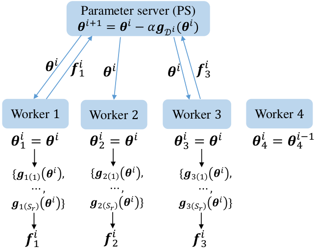
To elaborate on the communication and computation protocol, we define as the version of the model parameter that worker has available at iteration prior to computation. At each iteration , a subset of workers, denoted by , is selected to download the model parameter from the PS. As illustrated in Fig. 2, each selected worker sets , and computes the local partial gradients over all assigned data partitions. In contrast, each non-selected worker does not download the current model parameter from the PS, and it reuses the locally available parameter vector from the previous iteration by setting . As a result, the local parameter vector is different from global parameter vector for all workers .
The wall-clock time required to complete the computation of all local gradients at each worker is random, with mean , for some , proportional to the worker load, which is in turn proportional to the storage redundancy . Variables are assumed to be i.i.d. across the worker index and iteration index . This standard assumption is motivated by the fact that, in most deployments, the workers are similar machines that operate independently (see, e.g., [5, 8, 10, 12]). In this paper, we will consider as representative examples an exponential distribution with mean and a Pareto distribution with scale-shape parameter pair , where and are constants. The latter has a higher tail than the former, implying a larger probability of straggling workers.
In order to reduce the time per iteration, as illustrated in Fig. 2, the PS may only wait for a subset of active workers to complete their computations. Each worker uploads a function of the computed partial gradients at current iteration back to the PS. Based on the received functions , and possibly also previously received functions , with , the PS computes an estimate of the gradient. Note that each worker in subset downloads the model parameter but it does not upload a local update due to the excessive time elapsed for its computation. Similar to each worker in subset , the workers in subset also reuse the outdated gradients for the local parameter vector .
The PS then updates the model parameter via the rule in (2). The PS also keeps track of the workers’ parameter vectors . The next iteration then starts with the workers in subset downloading the updated model from the PS. The training continues until a convergence criterion is satisfied or a maximum number of iterations is reached.
Throughout this paper, by following [10, 38, 42], we make the following standard assumptions on the local loss functions for each data partition and on the overall loss function .
Assumption 1: The local loss functions are -smooth for , for some , that is, we have the inequalities
| (4) |
for all and ; and for , and the loss function is -smooth with . From (4), the smoothness parameters determine the rate of variability of the gradient of each local loss function . The parameters are assumed to be known, and they can be practically estimated using techniques such as those discussed in [43].
Assumption 2: is -strongly convex, or more generally, it satisfies the Polyak Łojasiewicz (PL) condition for some , i.e., it satisfies the inequality
| (5) |
for all , where is a minimum of . Note that the minimum is unique for strongly convex function. From (5), the norm of the gradient can be used as a measure of distance to the optimal value of the loss function.
II-A Performance Metrics
We are interested in studying the performance in terms of training accuracy, communication load, and computation load as a function of the wall-clock time. To this end, we start by defining the number of iterations of the SGD rule (2) carried out by time as
| (6) |
Note that is a random variable due to the randomness of the times and of the subsets . Furthermore, the quantity represents the time per iteration since the PS waits for all the workers in subset to finish their respective computations. For each iteration , the communication load is defined as the sum of the numbers of workers that download model parameters from the PS and of the numbers of workers that upload the computed gradients to the PS. It follows that the communication load as a function of time is given as
| (7) |
We also define the computation load as the total number of gradients per data point computed at the workers. The computation load at time is given by
| (8) |
since each worker in set computes local gradients. Note that the workers in may compute only partially the local gradients, but here we do not make this distinction since, in practice, this would require additional signaling from PS to the workers. Finally, the training loss optimality gap at time is given by
| (9) |
Beside the random tuple , we also consider the time complexity, the communication complexity, and the computation complexity, which are summary metrics that measure as the average time, communication load, and computation load needed to ensure an optimality gap equal to . Accordingly, defining as the (random) number of iterations needed to obtain an -optimality gap, also known as iteration complexity [10], , the wall clock time complexity is defined as
| (10) |
the communication complexity as
| (11) |
and the computation complexity as
| (12) |
We note that we have included in the wall-clock time only the durations of the computation steps, hence excluding the contribution of communications. This allows to more clearly highlight the trade-off between computing and communication. A compound wall-clock run-time metric that accounts for both computation and communication can be easily derived from the results in this paper.
III Background
III-A Gradient Coding (GC)
GC, introduced in [8], is an exact full-gradient descent approach, implementing rule (2) with , that aims at mitigating straggling workers by leveraging storage and computational redundancy. Prior to training, GC replicates each data partition times across the workers. To this end, dataset is first divided into partitions . Each partition is stored at workers, and we have partitions at each worker. Specifically, worker stores partition with , with and being the modulo- operation (see Fig. 3 for an example). At each iteration , all the workers download the model from the PS to execute the computations, i.e., we have (recall Fig. 2). Note that, for GC, we hence have the local parameter given as for all the workers. The PS waits only the fastest workers to finish their computations, yielding the subset , where is the th order statistic of the variables . To enable the recovery of the gradient at the PS, each of the worker in sends a designed linear combination of the computed partial gradients to the PS. The PS then computes a linear combination of the vectors so as to recover the full gradient . In order to guarantee the existence of linear encoding and decoding functions that enable the recovery of the full gradient for any set of workers, the inequality is necessary and sufficient [8].
As a special case of GC, if , the entire dataset can be stored at each worker. In this case, the PS can wait for the fastest worker only (), and no coding and decoding operations are needed.
Example: Consider workers, data partitions at each worker, and storage redundancy . GC allows the PS to wait only for the fastest workers since . As shown in Fig. 3, this is done by splitting dataset into partitions , and . Worker stores partitions and , while and worker 3 stores and . The three workers compute the linear functions indicated in Fig. 3. It can be easily seen that, by summing functions recevied from any two workers, the PS can recover the exact full gradient .
III-B Lazily Aggregated Gradient (LAG)
Lazily Aggregated Gradient (LAG), proposed in [10], is an approximate gradient descent scheme that judiciously selects the subset of active workers at each iteration in order to reduce communication and computation loads. Unlike GC, LAG does not require storage redundancy, and hence we have . We can also set without loss of generality and assign each worker a disjoint data partition , so that . The PS determines the subset of active workers at each iteration on the basis of the estimated change in the gradient for the local loss function corresponding to the data partition at worker as compared to the latest communicated gradient from the worker. Note that, since the subset is determined irrespective of the realization of the computation times, unlike GC, LAG is not tolerant to stragglers.
In the following, we provide a more detailed description of LAG. We specifically follow the LAG-PS strategy introduced in [10]. More precisely, in order to highlight the common elements with GC, the scheme described here is functionally equivalent to LAG-PS, but it differs from it in terms of the way operations are split between encoding functions computed at the workers and decoding functions evaluated at the PS (see Remark 1 below for details).
At each iteration , the PS first determines the subset by checking the following condition for each worker
| (13) |
where we recall that is the smoothness constant of the local function , while is some constant. By (4), the left-hand side of (13) represents a bound on the change in the gradient squared norm expected for the local loss at worker as compared to the last available gradient from the worker. The right-hand side of (13), by the rule (2), represents the per-server average contribution over the most recent iterations to the approximate gradient norm squared , scaled by a parameter . The PS selects the workers that satisfy condition (13), i.e., the workers that are expected to have a sizeable difference between the current local gradient and their more recently computed gradients, and hence may contribute more significantly to the model update (2). This yields the subset .
With the received parameter , each worker computes the local gradient in (3) and then sends the result to the PS. In contrast, for each unselected user in subset , which does not compute an update, the outdated partial gradients from iteration is reused. Note that we have . By combining both the computed gradients and the outdated gradients, the PS estimates the full gradient
| (14) |
The PS computes , and updates the variables and before moving to the next iteration.
Example: Consider again workers. As illustrated in Fig. 4, at each iteration , the PS checks condition (13) for each worker. Assume that only worker 1 satisfies it, and hence we have . Therefore, only worker 1 downloads the current model from the PS. It then computes the local gradient and uploads to the PS. Combining with the outdated partial gradients and of worker 2 and 3, the PS recovers the estimate . The PS then updates , as well as and for . The next iteration then continues with a check of condition (13) by the PS in the same way.
Remark 1
In the original LAG in [10], instead of uploading , each worker transmits to the PS the gradient change . The PS then estimates the full gradient by summing the vectors to the previous gradient estimate as [10, Eq. (6)]
| (15) |
The update (14) considered here yields by direct computation the equalities
| (16) |
where holds because we have for any at iteration . From (15) and (1), we can see that the described LAG and the original LAG in [10] are equivalent since they use the same gradient estimate in the update (2).
IV Lazily Aggregated Gradient Coding (LAGC)
In this section, we propose a strategy, named Lazily Aggregated Gradient Coding (LAGC), that aims at exploring the trade-off between the robustness to stragglers of GC and the computation and communication efficiency of LAG by generalizing both schemes. The idea is to cluster all the workers into groups; treat each group as a single worker in LAG; and, within each group, mitigate the effect of stragglers by applying computation redundancy as in GC. In a manner similar to LAG, the PS selects only groups of workers that have collectively large expected new contributions to the gradient. The trade-off between the robustness to stragglers of GC and the computation and communication efficiency of LAG can be controlled by selecting the size of the groups, with GC and LAG being two extreme special cases. In particular, increasing the size of the groups enhances the capability of LAGC to mitigate stragglers by utilizing storage redundancy within each group. Conversely, reducing the size of the groups gives the PS more flexibility on the selection of the subset of workers to activate at each iteration, hence potentially reducing the computation complexity.
To elaborate, LAGC divides all the workers into groups , each having workers, where design parameter is an integer divisor of . Dataset is split into partitions of equal size, with each partition assigned exclusively to group , for any . In each group, partition is assigned to the workers in by following GC. Accordingly, we further split into equal-size batches . Each partition is then stored at workers in each group. Specifically, the th worker stores partition for . Note that, when the design parameter is selected as , the workers’ storage redundancy is underused. Furthermore, if , all workers in a group can fully store the partition , and hence, as in LAG and as further discussed below, no coding is needed.
We denote as the model parameter available at all workers in group at iteration , i.e., we have . At each iteration , the PS determines the subset of groups to be activated first. To this end, the PS evaluates the condition
| (17) |
for all groups , where we write for the smoothness constant of the local function of each group . In a manner similar to (13), condition (17) is satisfied by groups that are expected to have a large new contribution to the model update (2). This is because, the right-hand side of (17), by the rule (2), represents the per-group average contribution over the most recent iterations to the approximate gradient norm squared ; while, by (4), the left-hand side of (17) represents a bound on the change in the gradient squared norm expected for the local loss at group as compared to the available gradient of the group at last iteration. The PS selects all the groups that satisfy condition (17), i.e., the subset of groups . All the workers in each group , with , download the parameter from the PS, and the subset of active workers is hence given as .
For each selected group with index , the PS only waits for the fastest workers to finish their computations. As in GC, in order to guarantee the recovery of the full local gradient for each group , the condition is necessary and sufficient [8]. As a result, we have the subset of workers uploading their gradients to the PS at iteration , where is the th order statistic of the variables . Note, in particular, that, if yielding , the PS can wait for the fastest worker in the group, i.e., . In fact, each worker can compute directly the gradient for the partition allocated to group . For the more general case that is not equal to , each of the non-straggling workers uploads a linear combination of the computed partial gradients and the PS decodes the local gradient by following GC.
Finally, by combining with the outdated gradients from the inactive groups, the PS estimates the full global gradient as
| (18) |
which is used in the update rule (2). The PS also updates the variables and . The full algorithm is summarized in Algorithm 1.
Remark 2
As discussed, LAGC generalizes both LAG and GC: when choosing and , LAGC reduces to GC, while setting recovers LAG. Intermediate values of yield novel schemes.
Remark 3
Setting the number of groups to be smaller or equal to the storage redundancy, i.e., , yields a novel scheme that does not require coding within each group, while still benefiting from both robustness to stragglers and reduced computation complexity. With this choice, each worker stores the entire data partition for group . Hence, for each selected group with , the PS only needs to wait for the fastest worker (i.e., ), since the latter can send the desired gradient directly to the PS. To highlight the fact that no coding is involved, we refer to this set of schemes as Grouped-LAG (G-LAG). We note that setting , and hence selecting all groups at all times, G-LAG reduces to Grouped-GD (G-GD) [9].
Example: Consider workers and storage redundancy . In this case, can take values or 3, apart from the cases and , corresponding to LAG and GC, respectively. For , we have the G-LAG scheme described in Remark 3, whereby each worker in each group can store the entire data partition of that group and no coding is necessary, as shown in Fig. 5(a). In the example of Fig. 5(a), the PS selects only group using condition (17), and the PS obtains directly from the fastest worker in . For , the workers are clustered into two groups and the partition for each group is divided into two parts, each stored at two workers with redundancy , as shown in Fig. 5(b). In the illustration of Fig. 5(b), only group 1 satisfies condition (17). Hence, worker and 3 in group download the model from the PS, and the PS waits for the fastest workers to finish their computations. GC is used to recover the gradient from group . By summing up the outdated partial , the PS estimates the global gradient as .
V Analysis
In this section, we analyze the time complexity (10), communication complexity (11), and computation complexity (12) of all the schemes considered above, which are summarized in Table II. Note that, as a reference, we also study standard Gradient Descent (GD), which is a special case of GC without data redundancy, i.e., with ; as well as G-GD, which, as seen, is an extreme case of G-LAG where all the groups are active at each iteration. The results of the analysis in this section are summarized in Section V-D via numerical illustrations.
In order to derive the mentioned metrics, we first discuss the iteration complexity in (6). A standard result is that GD has iteration complexity
| (19) |
with being the condition number for the training empirical loss (1) and being the difference between the loss at the initial iteration and the loss at the optimal point [44]. We note that this result is obtained by choosing a stepsize . By constructions, GC and G-GD have the same iteration complexity . For LAG, as shown in [10], by choosing the stepsize as , we have the iteration complexity
| (20) |
which shows the same scaling with and as GD. Finally, for LAGC, the iteration complexity is by construction equivalent to that of LAG with workers. In fact, since LAGC treats each group of workers as a single worker, its operation is equivalent to a system with a smaller number of workers. Given that the iteration complexity of LAG does not depend on the number of workers, we have .
| Coding | Adaptive selection | Grouping | |
|---|---|---|---|
| GD | |||
| GC [8] | |||
| LAG [10] | |||
| G-GD [9] | |||
| G-LAG [this paper] | |||
| LAGC [this paper] |
V-A Wall-clock Time Complexity
We proceed to analyze the average wall-clock time complexity (10). To elaborate, we define as the th order statistics of i.i.d. variables , that is, the th smallest value in the set , where and are two integers satisfying . The average can be written in closed form for the two representative distributions considered here. In particular, we have
| (21) |
for the case of exponential distribution with mean [45], where is the th harmonic number; and
| (22) |
for the case of Pareto distribution with scale-shape pair with , where is Gamma function given by [46]. Note that both averages (21) and (22) increase with the mean of each variable and with . To ease the notation, we also write in the following.
GD: The average run-time of each iteration for GD is given as , since the PS waits for all servers to complete their computations at each iteration and no computational redundancy is leveraged, i.e., . This yields the overall run-time
| (23) |
GC: With GC, at each iteration , the PS waits only for the set of the fastest workers to finish their computations, yielding the average run-time . As a result, the overall run-time is given as
| (24) |
Comparing with (23), GC can reduce the time complexity if .
LAG: At each iteration of the LAG scheme which assumes , all the selected workers in subset have to complete their computations, yielding the average run-time . From [10, Lemma 4], given an integer , a worker with smoothness parameter satisfying the inequalities
| (25) |
is selected in at most iterations. A larger smoothness constant, and hence a less sensitive gradient, cause a worker to be selected less frequently. Using this result, we can bound the average number of selected servers per iteration as
| (26) |
where we have defined the function with . Note that function indicates the fraction of the workers satisfying condition (25). Therefore, parameter increases when all smoothness constant decrease. From [10], we have that , i.e., . As proved in Appendix A, the bound (26) can be used in turn to bound the overall time as
| (27) |
Comparing with (23), we see that LAG can only decrease the time complexity as compared to GD if and the smoothness constant are large.
G-GD: Based on grouping, at each iteration , the PS waits for the fastest workers in each group to finish their computations. Hence, the run-time for each group is the th order statistic of the random times of the workers in group . In a manner similar to (21)-(22), we define to be the expectation of the th order statistics of the random variables , and we denote . Unlike (21)-(22), this expectation does not generally have a closed form, but it can be computed numerically as
| (28) |
where we have defined the Cumulative Distribution Function (CDF) of each variable [47]. With these definitions, the overall run-time of G-GD is given as
| (29) |
Based on (29), G-GD can reduce the time complexity if .
LAGC: At each iteration , LAGC selects a subset of groups with . Using the same approach discussed above from [10], the average group size can be upper bounded as
| (30) |
where we have defined the function , with and . This distribution has the same interpretation given above for function , with groups replacing workers. Similarly, we have that , i.e., . To allow all the selected groups in subset to complete the computations, the average run-time of each iteration is given as . As a result, the overall average run-time can be upper bounded as
| (31) |
Comparing with (23), LAGC can hence outperform GD in terms of time complexity if .
V-B Communication Complexity
We proceed to investigate the communication complexity.
GD: With the conventional GD, the overall communication load is given as
| (32) |
since all workers download and upload model parameters from the PS.
GC: At each iteration of GC, there are workers downloading the model parameter and workers uploading the computed results. Hence, the overall communication load is given as
| (33) |
Comparing (33) with (35), we observe that GC reduces the communication complexity by a factor , which can be as large as 2 if is small enough.
LAG: At each iteration of LAG, all the workers in subset download from the PS and also upload model parameters to the PS. Hence, the overall communication load is given as
| (34) |
with defined in (26). Since we have , LAG can reduce the communication complexity as long as is not too small.
G-GD: With G-GD, the overall communication load within iterations is given as
| (35) |
since all workers download the model parameters but only the fastest workers in each group upload the computed results. Hence, G-GD reduces the communication complexity as compared to GD by a factor that increases with the computation redundancy factor .
LAGC: At each iteration of LAGC, groups of workers are chosen to download the model parameter, which amount to . In each group, workers upload their computations, yielding . As a result, the overall communication complexity within iterations is given as
| (36) |
with defined in (30). Since the average number of selected workers for download and the number of selected workers for upload are both no larger than the total number of workers, LAGC can outperform GD in terms of communication complexity when is close to one.
V-C Computation Complexity
Finally, we evaluate the computation complexity (12).
GD: The overall computation complexity over iterations for GD is given as
| (37) |
since the gradient for each data point is computed as each iteration.
GC: With a data redundancy at the workers, the overall computation complexity of GC is given as
| (38) |
The computation load of GC is hence times that of GD.
LAG: The overall computation complexity of LAG is similarly bounded as
| (39) |
Therefore, LAG can reduce the computation complexity if is close to one.
G-GD: The overall computation complexity of G-GD is given as
| (40) |
yielding an increase equal to in computation complexity.
LAGC: Finally, the overall computation complexity of LAGC is bounded as
| (41) |
since we have the inequality due to adaptive selection, LAGC can reduce the computation complexity of GC when the average number of groups satisfies the inequality as long as .
V-D Numerical Illustration
We now provide an illustration of the relative performance of the considered schemes. To this end, we consider a linear regression model , where input is an input vector obtained by pre-processing a vectorized handwritten digit image from the MNIST dataset. Specifically, the MNIST training dataset of 60,000 examples is divided into partitions of equal size, each including images for each digit . Each partition , with is processed as in [10] such that the smoothness constant of the corresponding loss function is set to be equal . The loss function is given as , where is the input matrix for the th partition (with each input corresponding to a row of ) and the target vector is given as for a randomly generated ground-truth parameter vector with i.i.d. zero-mean unitary power Gaussian entries. We consider the most recent iterations to approximate the gradient norm square. Furthermore, for the computing times, the Pareto distribution has shape parameter and scale parameter , and the exponential distribution has mean parameter . We evaluate the complexity measures derived above — using the bounds (27), (31), (39), (41) for LAG and LAGC — for redundancy for GC and LAGC, as well as hyperparameters , , and . We also set for GC and for G-GD and LAGC with set to different values. Time, communication and computation complexities of GD, GC, LAC, G-GD, and LAGC for different values of with Pareto distribution and exponential distribution are shown in Fig. 6 and Fig. 7, respectively. As discussed, in both figures, when and , LAGC coincides with LAG and GC, respectively, while, when for , we have the (uncoded) G-LAG scheme in Remark 3.
We first consider computing times with Pareto distribution. The high tail of the Pareto distribution entails a high probability that some workers are significantly slower than the rest. As seen in Fig. 6, in this case, both G-GD and GC have a lower time complexity than both GD and LAG thanks to their robustness to stragglers (recall Table I): Although each active worker executes more computations, the reduced requirements on the number of workers that need to complete their computations offset the increased per-server computation load. However, this wall-clock time saving implies a trade-off with the computation complexity, which is increased. Furthermore, G-GD outperforms GC in all metrics, since more stragglers can be tolerated thanks to grouping for without increasing the computational redundancy. LAG has a larger wall-clock time complexity as compared to G-GD and GC, but it can significantly reduce both communication and computation complexities by selecting a reduced number of workers to be active. The proposed LAGC scheme is seen to be able to harness both the robustness to stragglers of GC and G-GD, which requires a larger , and the reduced communication and computation complexity of LAG, which requires a smaller . In fact, in line with the comparison between G-GD and GC, we observe that G-LAG — the special case of LAGC that only with grouping and adaptive selection — yields the best overall performance.
We now consider the performance under the exponential distribution for the workers’ computing times. This distribution has a lower tail and hence the workers have comparable computing times with a higher probability than for the Pareto distribution. In this case, in stark contrast to Fig. 6, Fig. 7 shows that GC does not improve the time complexity, since the cost resulting from computational redundancy does not offset the savings accrued thanks to the mitigation of stragglers. As compared to LAG, G-GD provides a reduction in wall-clock time due to its stronger ability to tolerate stragglers, implying a trade-off with the increasing computation complexity. LAG outperforms schemes based solely on grouping or coding in terms of communication and computation complexity. Finally, the proposed G-LAG outperforms all other schemes in terms of computation and time complexities while requiring a larger computation complexity than LAG.




VI Numerical Results
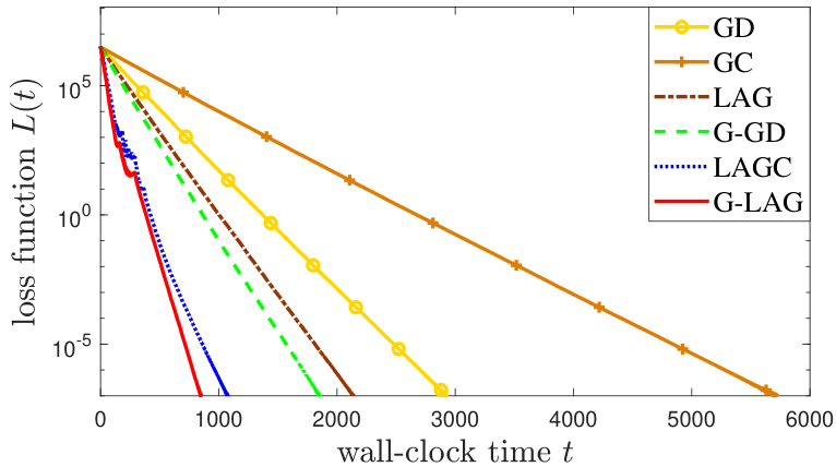
In this section, we present numerical examples in order to illustrate the loss function in (9), communication load in (7), and computation load in (8) as function of wall-clock time for the considered training strategies. We adopt the same linear regression set-up described in Section V-D with Pareto and exponential distributions for the random computing times of the workers. In Fig 8 and 9, we plot the mentioned metrics averaged over 100 random realization of the computing times for GD, GC, LAG, G-GD, LAGC with , and G-LAG with . We note that each curve terminates at the time when the -optimality is achieved.
Confirming the conclusion from the analysis in Section V-D, under Pareto computing times, the loss functions of GC, G-GD, LAGC, and G-LAG decrease significantly faster than GD and LAG thanks to their robustness to stragglers, as shown in Fig. 8, with G-LAG yielding the steepest descent. LAG is seen to be effective in reducing the communication and computation loads per unit of time. However, G-LAG yields a small overall communication complexity, at the cost of a large computation due to the smaller time for iteration afforded by its robustness to stragglers.
We now turn to considering exponential computing times. In this regard, Fig 9 verifies the conclusion based on the analysis in Section V-D that coding is not advantageous in terms of any performance metric with respect to GC. In contrast, G-GD can be significantly more time efficient due to its stronger robustness to stragglers. By using adaptive selection, the communication loads of LAG, LAGC and G-LAG increase with similar rates as a function of , but G-LAG has a smaller communication complexity due to the smaller time complexity. Finally, due to computational redundancy, G-LAG, GC, and LAGC have higher computation loads than the other schemes.
VII Conclusions
In this work, we explored the trade-off among wall-clock time, communication, and computation requirements for gradient-based distributed learning by leveraging coding, grouping, and adaptive selection. As summarized in Table I, both coding and grouping provide robustness to stragglers, while adaptive selection is beneficial to reduce communication and computation loads. We proposed two novel strategies that aim at integrating the benefits of both types of approaches. Through analysis and numerical results, we have concluded that, when the distribution of the computing times of the workers has a low tail, the advantage of straggler mitigation via coding does not compensate for the increased computation load even in terms of wall-clock run-time. In contrast, for both high- and low-tail distributions of the computing times, the proposed G-LAG was seen to strike a desirable balance in terms of wall-clock time and communication overhead, with only a limited increase in computation cost.
This work leaves open a number of research directions. First, it would be interesting to combine stochastic gradient coding [14, 15, 17] with grouping and adaptive selection. Second, the potential advantages of the techniques considered here should be reconsidered for asynchronous implementations, where any server can compute the gradient and send an update to the PS without waiting for the other servers [38]. Lastly, a related issue would be to introduce data privacy requirements [48].
Appendix A Proof of bounds (27) and (31)
Define as the Cumulative Distribution Function (CDF) of each variable . From [49, Lemma 2], we have the equality
| (42) |
From (42), since , the function has decreasing increments in , and hence it is discrete concave [50]. It follows that for any integers with , we have Jensen’s inequality
| (43) |
as long as is an integer. In order to apply (43), we define and . We then have the desired inequality in (27). Bound (31) follows from the same argument.
Acknowledgements
Jingjing Zhang and Osvaldo Simeone have received funding from the European Research Council (ERC) under the European Union’s Horizon 2020 Research and Innovation Programme (Grant Agreement No. 725731).
References
- [1] J. Dean, G. S. Corrado, R. Monga, and et al, “Large scale distributed deep networks,” in Proc. Advances in Neural Info. Process. Syst. (NeurIPS), Lake Tahoe, USA, Dec 2012, pp. 1223–1231.
- [2] M. Abadi, A. Agarwal, P. Barham, and et al, “Tensorflow: Large-scale machine learning on heterogeneous distributed systems,” 2015. [Online]. Available: http://download.tensorflow.org/paper/whitepaper2015.pdf
- [3] M. Zinkevich, M. Weimer, L. Li, and A. J. Smola, “Parallelized stochastic gradient descent,” in Proc. Advances in Neural Info. Process. Syst. (NeurIPS), Vancouver, Canada, 2010, pp. 2595–2603.
- [4] A. Smola and S. Narayanamurthy, “An architecture for parallel topic models,” The Proceedings of the VLDB Endowment (PVLDB), vol. 3, no. 1-2, pp. 703–710, Sep. 2010.
- [5] M. Li, D. G. Andersen, J. W. Park, and et al, “Scaling distributed machine learning with the parameter server,” in Proc. Symp. on Operating Systems Design and Implementation (OSDI), Denver, USA, 2014, pp. 583–598.
- [6] J. Dean and L. A. Barroso, “The tail at scale,” Communications of the ACM, vol. 56, no. 2, pp. 74–80, Feb 2013.
- [7] L. A. Barroso and U. Hoelzle, The Datacenter As a Computer: An Introduction to the Design of Warehouse-Scale Machines. Morgan and Claypool Publishers, 2009.
- [8] R. Tandon, Q. Lei, A. G. Dimakis, and N. Karampatziakis, “Gradient coding: Avoiding stragglers in distributed learning,” in Proc. Int. Conf. on Mach. Learn. (ICML), Australia, Sydney, Aug 2017, pp. 3368–3376.
- [9] E. Ozfatura, D. Gündüz, and S. Ulukus, “Gradient coding with clustering and multi-message communication.” [Online]. Available: http://arxiv.org/abs/1903.01974
- [10] T. Chen, G. Giannakis, T. Sun, and W. Yin, “LAG: Lazily aggregated gradient for communication-efficient distributed learning,” in Proc. Advances in Neural Info. Process. Syst. (NeurIPS), Montreal, Canada, Dec 2018, pp. 5050–5060.
- [11] J. Watt, R. Borhani, and A. K. Katsaggelos, Machine Learning Refined: Foundations, Algorithms, and Applications. New York, USA: Cambridge University Press, 2016.
- [12] M. Ye and E. Abbe, “Communication-computation efficient gradient coding,” in Proc. Int. Conf. on Machine Learning (ICML), Stockholm, Sweden, July 2018, pp. 5606–5615.
- [13] W. Halbawi, N. A. Ruhi, F. Salehi, and B. Hassibi, “Improving distributed gradient descent using Reed-Solomon codes,” Colorado, USA, June 2018, pp. 2027–2031.
- [14] N. Raviv, R. Tandon, A. Dimakis, and I. Tamo, “Gradient coding from cyclic MDS codes and expander graphs,” in Proc. Int. Conf. on Machine Learning (ICML), Stockholm, Sweden, July 2018, pp. 4302–4310.
- [15] Z. Charles, D. Papailiopoulos, and J. Ellenberg, “Approximate gradient coding via sparse random graphs.” [Online]. Available: https://arxiv.org/abs/1711.06771
- [16] S. Kadhe, O. O. Koyluoglu, and K. Ramchandran, “Gradient coding based on block designs for mitigating adversarial stragglers,” 2019. [Online]. Available: https://arxiv.org/abs/1904.13373
- [17] R. Bitar, M. Wootters, and S. E. Rouayheb, “Stochastic gradient coding for straggler mitigation in distributed learning,” 2019. [Online]. Available: https://arxiv.org/abs/1905.05383
- [18] H. Wang, Z. B. Charles, and D. S. Papailiopoulos, “Erasurehead: Distributed gradient descent without delays using approximate gradient coding,” 2019. [Online]. Available: https://arxiv.org/abs/1901.09671
- [19] R. K. Maity, A. S. Rawat, and A. Mazumdar, “Robust gradient descent via moment encoding with ldpc codes,” 2019. [Online]. Available: https://arxiv.org/abs/1805.08327
- [20] K. Lee, M. Lam, R. Pedarsani, D. Papailiopoulos, and K. Ramchandran, “Speeding up distributed machine learning using codes,” IEEE Trans. Inf. Theory, vol. 64, no. 3, pp. 1514–1529, March 2018.
- [21] K. Lee, C. Suh, and K. Ramchandran, “High-dimensional coded matrix multiplication,” in Proc. IEEE Int. Symp. Information Theory (ISIT), Aachen, Germany, June 2017, pp. 2418–2422.
- [22] Q. Yu, M. Maddah-Ali, and S. Avestimehr, “Polynomial codes: an optimal design for high-dimensional coded matrix multiplication,” in Proc. Advances in Neural Info. Process. Syst. (NeurIPS), Long Beach, US, 2017, pp. 4403–4413.
- [23] M. Fahim, H. Jeong, F. Haddadpour, S. Dutta, V. Cadambe, and P. Grover, “On the optimal recovery threshold of coded matrix multiplication,” in Proc. Allerton Conf. Communication, Control and Computing, Illinois, USA, Oct 2017, pp. 1264–1270.
- [24] S. Dutta, V. Cadambe, and P. Grover, “Short-dot: Computing large linear transforms distributedly using coded short dot products,” in Proc. Advances in Neural Info. Process. Syst. (NeurIPS), Barcelona, Spain, 2016, pp. 2100–2108.
- [25] H. Zhang, J. Li, K. Kara, D. Alistarh, J. Liu, and C. Zhang, “ZipML: Training linear models with end-to-end low precision, and a little bit of deep learning,” in Proc. of Int. Conf. on Machine Learning, Sydney, Australia, Aug 2017, pp. 4035–4043.
- [26] A. T. Suresh, F. X. Yu, S. Kumar, and H. B. McMahan, “Distributed mean estimation with limited communication,” in Proc. of Int. Conf. on Machine Learning, Sydney, Australia, Aug 2017, pp. 3329–3337.
- [27] J. Wangni, J. Wang, J. Liu, and T. Zhang, “Gradient sparsification for communication-efficient distributed optimization,” in Proc. Advances in Neural Info. Process. Syst. (NeurIPS) workshop, 2018, pp. 1306–1316.
- [28] M. Jaggi, V. Smith, M. Takac, J. Terhorst, S. Krishnan, T. Hofmann, and M. I. Jordan, “Communication-efficient distributed dual coordinate ascent,” in Proc. Advances in Neural Info. Process. Syst. (NeurIPS), Montreal, Canada, 2014, pp. 3068–3076.
- [29] C. Ma, J. Konečný, M. Jaggi, V. Smith, M. I. Jordan, P. Richtárik, and M. Takáč, “Distributed optimization with arbitrary local solvers,” Optimization Methods and Software, vol. 32, no. 4, pp. 813–848, 2017.
- [30] O. Shamir, N. Srebro, and T. Zhang, “Communication-efficient distributed optimization using an approximate newton-type method,” in Proc. of Int. Conf. on Machine Learning, Bejing, China, Jun 2014, pp. 1000–1008.
- [31] Y. Zhang and X. Lin, “DiSCO: Distributed optimization for self-concordant empirical loss,” in Proc. of Int. Conf. on Machine Learning, Lille, France, Jul 2015, pp. 362–370.
- [32] M. Jahani, X. He, C. Ma, A. Mokhtari, D. Mudigere, A. Ribeiro, and M. Takác, “Efficient distributed hessian free algorithm for large-scale empirical risk minimization via accumulating sample strategy,” 2018. [Online]. Available: http://arxiv.org/abs/1810.11507
- [33] L. Bottou, “Large-scale machine learning with stochastic gradient descent,” in Proc. of COMPSTAT’2010. Heidelberg, Germany: Physica-Verlag HD, 2010, pp. 177–186.
- [34] L. Bottou and O. Bousquet, “The tradeoffs of large scale learning,” in Proc. Advances in Neural Info. Process. Syst. (NeurIPS) workshop, 2007, pp. 161–168.
- [35] D. Alistarh, D. Grubic, J. Li, R. Tomioka, and M. Vojnovic, “QSGD: Communication-efficient sgd via gradient quantization and encoding,” in Proc. Advances in Neural Info. Process. Syst. (NeurIPS) workshop, Long Beach, USA, 2017, pp. 1709–1720.
- [36] J. Bernstein, Y.-X. Wang, K. Azizzadenesheli, and A. Anandkumar, “SIGNSGD: Compressed optimisation for non-convex problems,” in Proc. of the 35th Int. Conf. on Machine Learning (ICML), Stockholm, Sweden, 2018, pp. 1709–1720.
- [37] J. Tsitsiklis, D. Bertsekas, and M. Athans, “Distributed asynchronous deterministic and stochastic gradient optimization algorithms,” IEEE Trans. Automatic Control, vol. 31, no. 9, pp. 803–812, Sep 1986.
- [38] S. Dutta, G. Joshi, S. Ghosh, P. Dube, and P. Nagpurkar, “Slow and stale gradients can win the race: Error-runtime trade-offs in distributed SGD,” in Proc. Int. Conf. on Artificial Intelligence and Statistics (AISTATS), Lanzarote, Canary Islands, 2018, pp. 803–812.
- [39] B. Recht, C. Re, S. Wright, and F. Niu, “Hogwild: A lock-free approach to parallelizing stochastic gradient descent,” in Proc. Advances in Neural Info. Process. Syst. (NeurIPS) workshop, J. Shawe-Taylor, R. S. Zemel, P. L. Bartlett, F. Pereira, and K. Q. Weinberger, Eds., 2011, pp. 693–701.
- [40] J. Martens and R. Grosse, “Optimizing neural networks with kronecker-factored approximate curvature,” in Proc. of Int. Conf. on Machine Learning (ICML), Lille, France, 2015, pp. 2408–2417.
- [41] J. Ba, R. Grosse, and J. Martens, “Distributed second-order optimization using kronecker-factored approximations,” in Proc. of the Int. Conf. on Learning representations (ICLR), Toulon, France, 2017.
- [42] L. Bottou, F. E. Curtis, and J. Nocedal, “Optimization methods for large-scale machine learning,” 2016. [Online]. Available: https://arxiv.org/abs/1606.04838
- [43] G. R. Wood and B. P. Zhang, “Estimation of the lipschitz constant of a function,” Journal of Global Optimization, vol. 8, no. 1, pp. 91–103, Jan. 1996.
- [44] M. Schmidt, “Lecture slides: Rates of convergence.” [Online]. Available: https://www.cs.ubc.ca/ schmidtm/Courses/540-W18/L5.pdf
- [45] A. Mallick, M. Chaudhari, and G. Joshi, “Rateless codes for near-perfect load balancing in distributed matrix-vector multiplication.” [Online]. Available: http://arxiv.org/abs/1804.10331
- [46] K. Vännman, “Estimators based on order statistics from a pareto distribution,” Journal of the American Statistical Association, vol. 71, no. 355, pp. 704–708, 1976.
- [47] B. C. Arnold, N. Balakrishnan, and H. N. Nagaraja, A First Course in Order Statistics. SIAM, 2008.
- [48] K. Bonawitz, V. Ivanov, B. Kreuter, A. Marcedone, H. B. McMahan, S. Patel, D. Ramage, A. Segal, and K. Seth, “Practical secure aggregation for privacy-preserving machine learning,” in Proc. ACM SIGSAC Conference on Computer and Communications Security, Dallas, USA, 2017, pp. 1175–1191.
- [49] H. A. David, “Augmented order statistics and the biasing effect of outliers,” Statistics Probability Letters, vol. 36, no. 2, pp. 199–204, 1997.
- [50] K. Murota, Discrete Convex Analysis. SIAM, 2003.