High Throughput Polar Decoding Using Two-Staged Adaptive Successive Cancellation List Decoding

Polar codes [1] are a kind of linear block codes of length $N$. Without loss of generality, we assume $N$=$2^{n}$ in this work, where $n$ is an integer. Let $\textbf{u}_{N}$ and $\textbf{x}_{N}$ be the input source word and the output codeword of an $N$-bit binary frame, respectively, and the encoding process can be simply expressed by $\textbf{x}_{N}=\textbf{u}_{N}\cdot\text{{F}}^{\otimes n},$ in which $\text{{F}}^{\otimes n}$ is called the generator matrix that equals to the $n^{th}$ Kronecker power of the polarization matrix F=$\left[\begin{array}[]{cc}1&0\\ 1&1\end{array}\right]$. Due to the polarization effect, each bit in $\textbf{u}_{N}$ has a different reliability. An information set $\mathcal{A}$ is determined by finding the $K$ most reliable bits. These $K$ bits, called information bits, are used to transmit information. The complement of $\mathcal{A}$, $\mathcal{A}^{c}$, is defined as the frozen set, in which the bits are called the frozen bits and set to 0. If an $r$-bit CRC code is used, the last $r$ information bits are used to transmit the checksum generated from the other $K$-$r$ information bits, and the code rate of polar codes is $R=\frac{K-r}{N}$.

Successive cancellation decoding is a basic decoding algorithm of polar codes and has a low computational complexity of $\mathcal{O}(N\log N)$. Its decoding process is usually represented by a scheduling tree. An example for an $N$=4 polar code is shown in Fig. 2. It is a full binary tree with $n$+1 stages. The operands of SC decoding are the log-likelihood ratios (LLRs). The $i^{th}$ LLR at stage $s$ is denoted as $L_{i}^{s}$, where $i\in[0,N-1]$ and $s\in[0,n]$. Specifically, $L_{i}^{n}$s are the channel LLRs that are inputted to the tree from the root node at stage $n$. $L_{i}^{0}$s are LLRs corresponding to the $N$ leaf nodes and the hard decision of $u_{i}$, denoted as $\hat{u_{i}}$, is made according to

where $\Lambda_{i}$=$L_{i}^{0}$. To obtain these $\Lambda_{i}$s, the nodes in the scheduling tree are calculated as follows. A pair of sibling nodes at stage $s$ share $2^{s+1}$ LLR inputs from stage $s$+1 and both of them execute $2^{s}$ calculations in parallel. The left and right sibling nodes (denoted as F- and G-nodes) calculate the following F- and G-functions, respectively:

where $L_{a}$ and $L_{b}$ are the two input LLRs and $\hat{ps}$ for the G-function is a binary bit called partial-sum. (2) is a hardware-friendly version of F-function proposed in [3]. For a G-node at stage $s$, its partial-sums are obtained by

where $\hat{u}_{j}$ is the last decoded bit. According to (4), the partial-sums of a G-node has data dependancy on the $2^{s}$ decoded bits rooted at its sibling F-node. Thus, it can be seen that the decoding process of SC decoding follows a depth-first traversal of the scheduling tree.

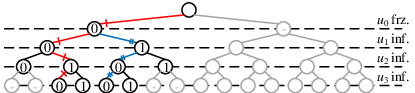
SCL decoding was proposed in [7, 9]. It has a significant performance gain over single SC decoding. Its decoding process can be regarded as a search problem on a binary decoding tree of depth-$N.$ Fig. 3a shows a decoding tree for a polar code of $N$=4. The $i^{th}$ source bit $u_{i}$, which corresponds to the $i^{th}$ leaf node in the scheduling tree, is mapped to the nodes at depth $i$+1 in the decoding tree. A path from the root node to a leaf node represents a candidate of decoded vector. For a parent node at depth $i$, its left and right children correspond to two different expansions of the partial decoded path with $u_{i}$=0 and 1, respectively. For example, the paths marked with single and double crosslines in Fig. 3a represent decoding vectors 0010 and 0100, respectively.

The decoding process begins from the root node. When the decoding process reaches a frozen bit $u_{i}$, such as $u_{0}$ in Fig. 3a, the sub-tree rooted at the right child is pruned (marked with light colour) as it does not contain any valid path, and the number of valid paths is unchanged. Otherwise, if $u_{i}$ is an information bit, the valid decoded paths are expanded to both sibling nodes and the number of valid paths in the list doubles. The number of the path candidates increases exponentially with respect to the number of decoded information bits. When a practical code length is used, the computational complexity will be too high to be implemented after a few bits are decoded. To limit the computational complexity, an LM operation is executed at each new depth to keep the number of survival paths to a predefined value $\mathcal{L}$ which is called the list size. In Fig. 3a, the lines with dark colours represent the paths that have been expanded during LM and those with crosslines represent the paths kept after LM.

The criterion of selecting survival paths during LM is their reliability measured by path metrics (PM). We denote the path metric of a path $l$ ($l\in[0,\mathcal{L}-1]$) after the decoding of bit $u_{i}$ as $\gamma_{i+1}^{k}$ where $k\in\{2l,2l$+1}. The PM is initialized as $\gamma_{0}^{0}$=0 and is updated based on bit-wise accumulation as [16]

Similar as (2), (5) is a hardware-friendly version of PM update. For a frozen bit, only one of (5) that satisfies $\hat{u_{i}}$=0 will be computed and the number of paths remains to be $\mathcal{L}$. As mentioned above, only the $\mathcal{L}$ left children nodes will be kept. Otherwise, both equations in (5) will be computed and the number of paths is doubled. After that, a list pruning operation will be executed, where all the $2\mathcal{L}$ PMs are sorted and the $\mathcal{L}$ paths with the smaller PMs will be kept in the list.

Recently, a variety of algorithms have been proposed to reduce the decoding latency of SCL by decoding multiple bits and executing their LM operation for only once. The algorithms in the literature can be divided into two different classes, multi-bit decoding (MBD) [22, 18, 19, 20] and special node decoding (SND) [27, 23, 26, 25, 24]. MBD decodes $M=2^{m}$ bits simultaneously, where $M$ is a fixed and predefined value. The decoding tree of MBD is modified to a full $2^{M}$-ary tree as shown in Fig. 3b, in which $M$=2. LM is still executed at each depth of this tree for each $M$ bits. SND, on the other hand, runs simplified LM algorithms for variable-length sub-codes that matches special code patterns. Fig. 3c shows the decoding tree modified for SND, in which rate-1 sub-code, a sub-code with only information bits, is used to simplify the decoding. Fewer paths are expanded from each survival path in SND and hence the computational complexity is reduced.

Adaptive SCL with CRC was proposed in [10] and the algorithm is summarised in Algorithm 1. Each time, a new codeword which contains $N$ LLRs is inputted for decoding. A-SCL starts with an SCL of $\mathcal{L}$=1, i.e., a single SC. If there are some decoded vectors that pass CRC at the end of decoding, the one with the highest reliability is chosen as output. Otherwise, the list size is doubled and the codeword is decoded again by an SCL with the new list size. Usually, a predefined $\mathcal{L}_{\text{max}}$ is used to limit the computational complexity, that is, after the decoding using an SCL with $\mathcal{L}_{\text{max}}$, the decoding terminates even when there is no valid candidate. From [10], the error correction performance of A-SCL is the same as that of an SCL with $\mathcal{L}_{\text{max}}$. At the same time, as most of the valid decoded vectors can be obtained using SCL with smaller list sizes, the average list size $\bar{\mathcal{L}}$ of A-SCL is much smaller than $\mathcal{L}_{\text{max}}$. An example for a polar code of $(N,K,r)$=$(1024,512,24)$ polar code is shown in Table I, in which $\bar{\mathcal{L}}\ll\mathcal{L}_{\text{max}}$=32 . As SCL with a smaller list size has a higher decoding speed, the average decoding speed of A-SCL is much higher than that of SCL.

However, if we directly implement the A-SCL algorithm in hardware, the following issues need to be addressed:

• •

  In an A-SCL decoding, different codewords may be decoded by SCL with different list sizes and SCL with a larger list size has a much larger latency. The decoding latency varies from frame to frame, so the system latency is not fixed. Because of that, a directly-mapped architecture may not be able to support applications that need to have a constant transmission data rate and latency, such as the channel coding blocks in communication systems.

• •

  A directly-mapped architecture is required to support multiple SCL decodings with list sizes $\mathcal{L}$ ranging from 1 to $\mathcal{L}_{\text{max}}$. This increases the design effort and also the hardware complexity. A simplified A-SCL decoding was proposed for accelerating software polar decoding [26], in which only one single SC and one SCL with $\mathcal{L_{\text{max}}}$ is used. However, as shown in Table I, its $\bar{\mathcal{L}}$ is larger than that of the original A-SCL, which means the achievable throughput gain is much less than that of the original A-SCL decoding. Moreover, simplified A-SCL does not support constant transmission data rate as well.

• •

  The throughput of A-SCL is not a constant under different channel conditions. As shown in Table I, the average list sizes of A-SCL decoding increase when the channel condition deteriorates as more frames need to be decoded multiple times, which indicates the throughput could be affected accordingly. It is also shown in [26] that a software-based simplified A-SCL decoder suffers from a 20x throughput reduction when the signal-to-noise ratio (SNR) is reduced by 1 dB. To adjust the data rate according to the channel condition, the transmitter side in a real system needs to know the channel SNR in real time, which increases the difficulty of system implementation.

To design a hardware-friendly A-SCL algorithm, we take reference from variable-iteration decoders for LDPC codes [31, 32, 33]. An additional buffer is employed at the input of the iterative decoder, in which the newly received codeword can be stored temporarily before the current decoding is finished. By doing so, the iterative decoder can use different decoding iterations to achieve decoding convergence and support constant transmission data rate at the same time. In the next section, we will propose a two-staged A-SCL decoding which solves the problems mentioned above with the help of some buffers and is hence suitable for hardware implementation.

As mentioned in Section II-D, the average list size and the error correction performance of A-SCL algorithm follows that of single SC and SCL with $\mathcal{L}_{\text{max}}$, respectively. Based on this observation, we propose a hardware-friendly TA-SCL whose algorithm is described as below.

The block diagram of TA-SCL and its timing schedule are shown in Fig. 4 and Fig. 5a, respectively. Basically, it includes two SCL decodings, which are an SCL decoding with small list size (not necessarily to be 1), denoted as $\mathbf{D}_{s}$, and an SCL decoding with large list size $\mathcal{L}_{\text{max}}$, denoted as $\mathbf{D}_{l}$. Each input codeword from the channel is first decoded by $\mathbf{D}_{s}$. If none of the candidates in the list passes CRC after this decoding, e.g. fr.1 in Fig. 5a, the current codeword will be decoded again by $\mathbf{D}_{l}$. This decoding usually takes longer time than decoding using $\mathbf{D}_{s}$. Nevertheless, $\mathbf{D}_{l}$ runs concurrently with $\mathbf{D}_{s}$ so that $\mathbf{D}_{s}$ starts decoding the next codeword immediately. Most of the time, $\mathbf{D}_{s}$ can decode the input codewords correctly and $\mathbf{D}_{l}$ becomes idle when the current decoding process finishes. However, if the channel is subject to burst errors, it is possible that a new codeword cannot be correctly decoded by $\mathbf{D}_{s}$ and the decoding in $\mathbf{D}_{l}$ has not finished yet. To deal with this, an LLR buffer is needed to store the LLRs of the codeword from $\mathbf{D}_{s}$ temporarily, such as fr.2, fr.3, fr.4 and fr.6 shown in Fig. 5a. An output buffer is also needed to re-order the decoded vectors as the codeword may be decoded out of order. For example, fr.7~fr.13 are stored in the output buffer until the decoding of fr.6 finishes.

The major difference between TA-SCL and A-SCL, either the original one or the simplified one, is that $\mathbf{D}_{s}$ can decode the next codeword from the channel input immediately instead of waiting for $\mathbf{D}_{l}$ to finish decoding the current codeword with the help of LLR buffer. The continuous running of $\mathbf{D}_{s}$ and LLR storage in the buffer permit the data to be transmitted at a constant data rate which is equal to the decoding throughput of $\mathbf{D}_{s}$ regardless of the SNR of the channel, while the decoding performance is guaranteed by $\mathbf{D}_{l}$. Also, TA-SCL benefits the hardware complexity as only two SCL decoders need to be implemented on hardware. The issues mentioned in Section II-D are hence solved.

If we have unlimited buffer resources, the decoding performance of TA-SCL will be the same as that of $\mathbf{D}_{l}$. However, in actual hardware implementation, the buffer size is limited and buffer overflow will happen, as shown in Fig. 5b. It happens when a new codeword needs to be stored in the LLR buffer but the buffer is full and decoding in $\mathbf{D}_{l}$ has not finished yet. To deal with buffer overflow, either the codeword in $\mathbf{D}_{s}$ or $\mathbf{D}_{l}$ would be thrown away and the incorrect decoding results from $\mathbf{D}_{s}$ will be used as the final output decoded vector of the corresponding codeword. Thus, the block error rate (BLER) of $\mathbf{D}_{\text{TA}}$, denoted as $\epsilon_{\mathbf{D}_{\text{TA}}}$, is bounded by

where the upper limit is the sum of the BLER of $\mathbf{D}_{l}$ and the probability of buffer overflow. Obviously, it is important to prevent buffer overflow in order to reduce performance loss which is defined as

In summary, the benefits of TA-SCL on hardware comes at the cost of error correction performance loss. To obtain the best tradeoff among performance, hardware usage and throughput, an analytical model of $\mathbf{D}_{\text{TA}}$ will be introduced next to obtain the relationship between Pr(Overflow) and the parameters of $\mathbf{D}_{\text{TA}}$ in the next sub-section. Before that, we define the design parameters of TA-SCL as follows.

• •

  $\mathcal{L}_{s}/\mathcal{L}_{l}$: list sizes of $\mathbf{D}_{s}$ /$\mathbf{D}_{l}$ .

• •

  $\epsilon_{s}/\epsilon_{l}$: BLERs of $\mathbf{D}_{s}$ /$\mathbf{D}_{l}$ .

• •

  $t_{s}/t_{l}$: decoding time of each codeword using $\mathbf{D}_{s}$ /$\mathbf{D}_{l}$ .

• •

  $\beta$: speed gain, i.e., $\frac{t_{l}}{t_{s}}$. In this work, $\beta$ is not limited to integer value and can be any rational number, which is given by $\beta=\frac{\beta_{n}}{\beta_{d}},$ where $\beta_{n},\beta_{d}\in\mathbb{Z}^{+}$ and $\beta_{n}\bot\beta_{d}$, i.e., $\beta_{n}$ and $\beta_{d}$ are co-prime.

• •

  $\zeta$: size of the LLR buffer, which equals to the number of codewords that can be stored in the buffer. In this work, we assume $\zeta\geq 1$ and $\zeta\in\mathbb{Z}^{+}$.

We also denote a TA-SCL decoding whose speed gain is $\beta$ and buffer size is $\zeta$ as $\mathbf{D}_{\text{TA}}(\beta,\zeta)$. The TA-SCL decoding in the example shown in Fig. 5a and 5b hence can be described as $\mathbf{D}_{\text{TA}}(3,\infty)$ and $\mathbf{D}_{\text{TA}}(3,1)$, respectively, and the corresponding $\mathbf{D}_{l}$ needs $3t_{s}$ to decode a codeword.

In this sub-section, we model the behavior of $\mathbf{D}_{\text{TA}}(\beta,\zeta)$ on B-DMC. Without loss of generality, we assume the channel is an additive white Gaussian noise (AWGN) channel. We first introduce the states that the decoder can operate at. We define the number of codewords currently stored in the LLR buffer as $i_{\zeta}$ and the remaining time required to finish the decoding of the current codeword in $\mathbf{D}_{l}$ as $i_{\beta}$ which is an integer multiple of $\frac{t_{s}}{\beta_{d}}$. Each codeword in the LLR buffer needs $\beta t_{s}$ to decode. Then, the state of TA-SCL is defined as

which is actually the total time required to clear the buffer in terms of $t_{s}$. For a $\mathbf{D}_{\text{TA}}(\beta,\zeta)$, there are $\mathcal{S}$=$\beta_{n}\zeta$+$\beta_{n}$+1 states in total. The $\mathcal{S}$ states can be categorized into the following groups according to whether buffer flow will happen.

• •

  Hazard states: The states that the LLR buffer is full and the current codeword decoded by $\mathbf{D}_{l}$ cannot be finished within $t_{s}$, which means $i_{\zeta}$=$\zeta$ and $i_{\beta}$>$\beta_{d}$. Buffer overflow will occur if $\mathbf{D}_{s}$ cannot decode the next codeword correctly. The codeword in $\mathbf{D}_{s}$ will be thrown away as this allows $\mathbf{D}_{l}$ to decode as many codewords as possible without any interruption.

• •

  Safe/Idle states: In contrast with the hazard states, these states do not have overflow hazard as the LLR buffer has enough space for a codeword that cannot be correctly decoded by $\mathbf{D}_{s}$. The transitions in idle states are a little different from those in safe states in the sense that $\mathbf{D}_{l}$ will finish its decoding and become idle during this $t_{s}$.

We show an example for $\mathbf{D}_{\text{TA}}(3,1)$ in Fig. 6a, where the black and white arrows represent the probabilities of $\epsilon_{s}$ and $\epsilon_{s}^{\prime}$=1-$\epsilon_{s}$, respectively. The first three columns show $i_{\beta}$, $i_{\zeta}$ and $X_{\tau}$, respectively. Typical transitions from hazard, safe and idle states are marked with “H”, “S” and “I” in the figure, respectively. The number of these states and their transitions are summarized in Fig. 6b. After defining these states, we introduce the modeling of TA-SCL by Proposition 1.

In this sub-section, we study the relationships between the error correction performance of TA-SCL decoding and its design parameters based on the proposed model. Simulation results are presented to verify the analysis numerically. A polar code of $(N,K,r)$=$(1024,512,24)$ is used for simulation over an AWGN channel, which is the same as that used in [22]. The low-latency hardware-friendly decoding algorithm proposed in [22], multi-bit DTS (MB-DTS), is used for $\textbf{D}_{l}$ with $\mathcal{L}_{l}$=32 as TA-SCL is targeting for hardware-based applications.

Instead of directly study the relationships of the design parameters with $\epsilon_{\mathbf{D}_{\text{TA}}}$, we first study their relationships with Pr(Overflow) with the help of the derived model.

The proposed architecture of TA-SCL decoder is shown in Fig. 9. It consists of four major sub-blocks: two constituent SCL decoders for $\mathbf{D}_{s}$ and $\mathbf{D}_{l}$, an LLR buffer and an output buffer. Data width of each connection is also marked in Fig. 9, where $P$ is called parallelism factor, i.e., the maximum number of F- or G-nodes that can be executed at the same time in $\mathbf{D}_{l}$, and $Q$ is the number of quantization bits for the LLR values. Details of each sub-block is introduced as below.

To support a high speed gain $\beta$, the architecture of $\mathbf{D}_{s}$ should have a very low decoding latency. Empirically, a $\mathbf{D}_{s}$ with $\mathcal{L}_{s}\leq 2$ provides error correction performance that is good enough to achieve a very low Pr(Overflow) and $\epsilon_{\textbf{D}_{\text{TA}}}$, and a larger $\mathcal{L}_{s}$ brings little performance gain but large overhead on timing and hardware complexity. Hence, a low-latency SCL decoding scheme targeting for $\mathcal{L}_{s}$=2 is used in the proposed TA-SCL architecture. It will be introduced in Section IV-C in detail. The memory usage of $\mathbf{D}_{s}$ is shown in Fig. 9. We only show the major memories which dominate the overall memory usage. The LLR memory stores both the channel LLRs and the calculated LLRs during decoding. The channel LLR memory have $NQ$ bits. It is also re-used for the storage of the calculated LLRs from the G-node at stage $n$-1. The calculated LLRs from the G-nodes at the other stages require about $\mathcal{L}_{s}\cdot 2\cdot\frac{NQ}{2}$ bits for storage in total [22]. The calculated LLRs of F-nodes at different stages can share a $\frac{NQ}{2}$-bit memory as they will be used only once in the next clock cycle directly and do not need to be stored afterwards [3, 22]. The partial-sum memory and path memory requires $\mathcal{L}_{s}\cdot\frac{N}{2}$ bits and $\mathcal{L}_{s}\cdot N$ bits, respectively. This architecture can also be configured for $\mathcal{L}_{s}$=1, and the corresponding memory usage is slightly larger than half of that of $\mathbf{D}_{s}$ with $\mathcal{L}_{s}$=2.

For $\mathbf{D}_{l}$, we use the architecture proposed in our previous work [22] and the details will not be discussed here. The sizes of LLR memory, partial-sum memory and path memory are $[(\mathcal{L}_{l}+1)N+3\mathcal{L}_{l}P]\cdot Q$ bits, $\mathcal{L}_{l}\cdot\frac{N}{2}$ bits and $\mathcal{L}_{l}\cdot N$ bits, respectively. The number of processing elements (PE) for each path in $\mathbf{D}_{l}$ equals to $P$.

The LLR buffer is implemented by a simple one-read one-write dual-port SRAM. The incoming channel LLR values will be written to the channel LLR memory in $\mathbf{D}_{s}$ and the LLR buffer at the same time. If $\mathbf{D}_{s}$ could not decode the frame correctly, this frame data will be kept in the LLR buffer for $\mathbf{D}_{l}$ decoding. Otherwise, it will be overwritten by the next frame. Thus the total size of the LLR buffer is $\zeta$+1 frame where $\zeta$ is the number of buffer required for storing the frame data for $\mathbf{D}_{l}$ as discussed in the analytical model and the additional buffer is holding the current frame data being decoded by $\mathbf{D}_{s}$. The size of LLR buffer is hence $NQ\cdot(\zeta$+1) bits. The width of each port is $2PQ$ bits. This parallelism matches with the I/O ports of $\mathbf{D}_{l}$ [22].

The output buffer is implemented by a true dual-port SRAM of which both ports can be used for reading or writing. It is used to align the output order to be the same as the input sequence because the decoding of the frames can be out of order. All the decoding results from $\mathbf{D}_{s}$ will be temporarily stored in this buffer. The results will be overwriten if the corresponding codeword is decoded by $\mathbf{D}_{l}$. Considering the worst case that a TA-SCL reaches the maximum state, the frame just stored into the LLR buffer and could not be decoded by $\mathbf{D}_{s}$ correctly will be decoded by $\mathbf{D}_{l}$ after $(\beta\zeta$+$\beta)\cdot\mathcal{C}_{s}$ clock cycles. All the decoding results of the codewords inputted after this frame need to be temporarily stored in the output buffer. So the output buffer needs to accommodate at most $\left\lceil\beta\zeta+\beta\right\rceil$ frames theoretically. In the real design, the output buffer needs to store $\left\lfloor\beta\zeta+\beta+1\right\rfloor$ frames, i.e, one more frame of the decoded vectors needs to be stored if $\beta\zeta$+$\beta$ is an integer, and the reason will be explained in Section IV-B. The size of the output buffer is hence $N\cdot\left\lfloor\beta\zeta+\beta+1\right\rfloor$ bits.

The memory usage of TA-SCL is summarized in Table II according to the analysis above. The hardware complexity overhead of TA-SCL over the traditional architecture for $\mathbf{D}_{l}$ comes from $\mathbf{D}_{s}$ and the two buffers, which is dominated by the memory overhead. As an example, the memory overhead of $\mathbf{D}_{\text{TA}}(3,3)$ (the one in Fig. 8a) is also shown in Table II and the overhead is around 20%. More accurate experimental results on hardware usage will be presented in Section V.

The timing schedule of TA-SCL architecture is illustrated in Fig. 10 with an example for $\mathbf{D}_{\text{TA}}(\frac{5}{2},1)$. Each line represents a decoding process or a data flow in Fig. 9, as marked with circled letters. The number shown in the waveforms represent the frame indices.

The first and third rows represent the decoding operations of $\mathbf{D}_{s}$ and $\mathbf{D}_{l}$, respectively, which are similar as the timing schedule shown in Fig. 5. The first $\mathcal{C}_{\text{rw}}\triangleq N/2P$ clock cycles are used to load the input channel LLRs. The periods filled with “//”, “\\” and “X” stripes represent the LLR loading time for $\mathbf{D}_{s}$, for $\mathbf{D}_{l}$ and for both, respectively. The second and fourth rows represent the operations of sending the decoding results from $\mathbf{D}_{s}$ and $\mathbf{D}_{l}$ to the output buffer, respectively. These two operations are executed concurrectly with the loading operations of the next codeword to be decoded. The fifth row shows when the final output results are generated from the output buffer. From the timing schedule, it can be seen that the final decoding results of any codeword will be available after $\mathcal{C}_{s}$+$\mathcal{C}_{s}$$\cdot(\beta\zeta$+$\beta$)+$\mathcal{C}_{\text{rw}}$ clock cycles when the corresponding LLRs are inputted to the decoder. The first term is caused by $\mathbf{D}_{s}$. The second term is dictated by the worst case discussed in Section IV-A. The third term is added to avoid potential memory collision as circled in Fig. 10: the decoded data is read out from the output buffer only after the two decoders send the decoded results to the output buffer. This is also the reason why we need space for one more frame as mentioned in Section IV-A. As an example, the system latency of $\mathbf{D}_{\text{TA}}(\frac{5}{2},1)$ in Fig. 9 is $6\mathcal{C}_{s}$+$\mathcal{C}_{\text{rw}}$ clock cycles.

In this section, we introduce a low-latency SCL (LL-SCL) decoding scheme customized for $\mathbf{D}_{s}$ with $\mathcal{L}_{s}\leq$2 such that $\mathbf{D}_{s}$ can support a large speed gain. It combines several state-of-the-art low-latency decoding schemes for SCL decoding, including G-node look-ahead scheme [6], multi-bit decoding (MBD) [19] and special node decoding (SND) [24, 25]. Specifically, LL-SCL can be divided into the following two parts.

• •

  SC calculations at stages not lower than stage $m$=$\log M_{s}$ ($M_{s}$ is the number of merged bits for MBD in $\mathbf{D}_{s}$) are calculated by normal SC algorithm with the full parallelism, i.e., $\frac{N}{2}$ PEs are used and any node in the scheduling tree takes only one clock cycle. Moreover, G-node look-ahead scheme [6] is used so that each pair of sibling nodes are calculated simultaneously and half of the latency is saved. Thus, the decoding latency of this part is $\frac{N}{M_{s}}$-1 clock cycles.

• •

  SC calculations at the low stages are replaced with MBD which decodes $M_{s}$ bits in the same sub-tree rooted at stage $m$ simultaneously. According to [19], given a certain number of frozen bit, there is only one code pattern for the $M_{s}$-bit sub-codes. So totally there are only $M_{s}$+1 different code patterns. To reduce the decoding latency, the decoding scheme for each code pattern is designed as follows. These $M_{s}$+1 code patterns are divided into multiple special nodes as shown in Table III where $T$ is the number of bits in each special node. The corresponding numbers of information bits and frozen bits are also listed. Rate-0, rate-1, repetition (Rep.) and single parity check (SPC) nodes are decoded according to the schemes presented in [26, 24, 25]. Rep2/SPC2 nodes can be divided into two Rep./SPC nodes with half of the lengths which can be decoded concurrently. Thus, each special node can be decoded by SND within one clock cycle. The number of paths is doubled after a special node is decoded. Different from the traditional SCL decoding, all the expanded paths are kept temporarily. List pruning is not executed until the end of each $M_{s}$-bit sub-code, which takes another clock cycle. Thus, an $M_{s}$-bit sub-code that can be divided into $M_{\text{SN}}$ special nodes requires $M_{\text{SN}}$+1 clock cycles to decode, except for $M_{s}$-bit rate-0 and rate-1 nodes which do not need a sorting operation and only take 1 clock cycle.

The total decoding latency of the LL-SCL decoding scheme is

where $\mathcal{C}_{\text{rw}}$ is the LLR loading latency and $\mathcal{F}_{i}$ is the number of frozen bits in the $i^{th}$ $M_{s}$-bit sub-code, $M_{\text{SN}}(\mathcal{F}_{i})$ and $\mathcal{C}_{\text{sort}}(\mathcal{F}_{i})$ are the decoding clock cycles for SND and sorting of the code pattern corresponding to $\mathcal{F}_{i}$, respectively. For $\mathcal{L}_{s}$=2,

For $\mathcal{L}_{s}$=1, the sorting operation for list pruning is unnecessary. Hence, $\mathcal{C}_{\text{sort}}(\mathcal{F}_{i})$=0 for $\mathcal{L}_{s}$=1, which indicates the throughput can be increased by using conventional SC decoding as $\mathbf{D}_{s}$.

The top level architecture of LL-SCL is shown in Fig. 11. For high stages, the SCL architecture [16] uses a PE array with $\frac{N}{4}$ PEs for each path. As the calculations at the highest stage $n$-1, which requires $\frac{N}{2}$ PEs to compute, are the same for both paths, they can use the two PE arrays from the two paths to accomplish. For low stages, $\text{max}(M_{\text{SN}})$ stages of SND blocks and a radix-$2^{\text{max}(M_{\text{SN}})+1}$ sorter are implemented in a feedforward manner, which are directly mapped from the decoding schemes introduced above. The architecture can be configured for $\mathcal{L}_{s}$=1 by simply disabling some of the blocks as shown in Fig. 11.

In this sub-section, we demonstrate the speed gain and the error correction performance of the proposed architectures. We apply TA-SCL decoding on several polar codes with different code lengths and code rates as shown in Table IV for illustration. These codes are similar to those chosen for the 5G eMBB control channel [8]. $\mathcal{P}_{1}$ is the same as the one used in [22] and similar to those presented in many existing works [24, 23]. $\mathcal{P}_{2}$ and $\mathcal{P}_{3}$ have different code rate and code length, respectively, and are used as examples to show the flexibility of TA-SCL decoding.

Table IV summarizes code characteristics and the number of cycles required for the corresponding $\mathbf{D}_{s}$ and $\mathbf{D}_{l}$. $|\mathcal{A}_{r}|$ is the number of reliable bits for the MB-DTS in the corresponding $\mathbf{D}_{l}$ [22]. For $\mathbf{D}_{s}$, MBD is applied to each 16-bit sub-codes, i.e., $M_{s}$=16, which means there are 17 code patterns in total. The number of special nodes in each code pattern and hence the number of cycles required for decoding is

As $\text{max}(M_{\text{SN}})$=3, the decoding latency of a sub-code varies from one to four clock cycles according to (19) and (20). As shown in part II of Table IV, these code patterns are divided into four different groups according to their decoding latency as shown in the brackets. The numbers of sub-codes in each group are then shown in the table, with which the decoding latency of $\mathbf{D}_{s}$ can be calculated according to (18) and presented in part III. For $\mathbf{D}_{l}$, MB-DTS is applied to sub-codes with a maximum length of $M_{l}$=4 and $P$=64 PEs are used for each path. Its total latency is calculated according to[22] and the results are shown in part IV. With the selected $M_{s}$ and $M_{l}$, the critical path delays of $\mathbf{D}_{s}$ and $\mathbf{D}_{l}$ are similar (both require 4~5 stages of adders delay) and the decoding latency can be minimized.

Based on the parameters shown in Table IV, we can design the TA-SCL decoders for $\mathcal{P}_{1}$~$\mathcal{P}_{3}$ to meet different requirements of error correction performance and speed gain. Some designs are listed in Table V. If we want to target for a TA-SCL decoder that has good decoding performance across a wide SNR range, as shown in Fig. 8, $\mathcal{L}_{s}$=2 should be used. $\mathbf{D}_{1}$, $\mathbf{D}_{2}$ and $\mathbf{D}_{3}$ shown in Table V are the designs for $\mathcal{P}_{1}$, $\mathcal{P}_{2}$ and $\mathcal{P}_{3}$, respectively, with $\mathcal{L}_{s}$=2 and $\mathcal{L}_{l}$=32. To determine the values of $\beta$ and $\zeta$ for each design, we set the maximum performance loss $\delta$ at a BLER of $10^{-2}$ to be 30%. $\beta$ is then calculated according to (16) and $\zeta$ is obtained by using the design flow presented in Section III-D. It can be observed from Table V that the speed gain is 3x~3.5x for these decoders. The error correction performance of these decoders on AWGN channel are simulated using both floating-point and fixed-point numbers and the results are shown in Fig. 12a-12c. The quantization schemes for $\mathbf{D}_{s}$ are $Q_{s,\text{LLR}}$=7 and $Q_{s,\text{PM}}$=8 so that the performance loss due to quantization error is reduced to the minimum and this is essential to avoid performance loss for the TA-SCL decoding as analysed in Section III. The quantization schemes for $\mathbf{D}_{l}$ are $Q_{l,\text{LLR}}$=6 and $Q_{l,\text{PM}}$=8 to achieve a balance between performance loss and hardware complexity. It can be seen that the fixed-point simulation results of TA-SCL decoding has negligible performance degradation (<0.05dB) compared with the floating-point results of $\mathbf{D}_{l}$ at the BLER of $10^{-2}$.

For some applications that only need to work at high SNR range but require a high throughput, we can use a $\mathbf{D}_{\text{TA}}$ with $\mathcal{L}_{s}$=1. We illustrate the performance of such a decoder with an example of $\mathbf{D}_{4}$ shown in Table V for $\mathcal{P}_{1}$. The decoding latency of $\mathbf{D}_{s}$ with $\mathcal{L}_{s}$=1 is 32 clock cycles fewer than that of $\mathbf{D}_{s}$ with $\mathcal{L}_{s}$=2. Consequently, $\mathbf{D}_{4}$ can achieve 0.6x more speed gain compared with $\mathbf{D}_{1}$. The error correction performance of $\mathbf{D}_{4}$ is shown in Fig. 12d. As $\epsilon_{s}$ and hence Pr(Overflow) is large at a lower SNR, we set the maximum performance loss $\delta$ at a lower BLER, i.e., a higher SNR. In this case, $\delta$ is set to be 30% at a BLER of $10^{-3}$ and the LLR buffer size $\zeta$ is equal to 6 to achieve this performance .

For some applications that can trade the error correction performance with lower decoding complexity, $\mathcal{L}_{l}$ can be smaller than 32 [22]. $\mathbf{D}_{5}$ shown in Table V is an example for $\mathcal{P}_{1}$. This design has the same design parameters, $\beta$ and $\zeta$, as those of $\mathbf{D}_{1}$. The hardware complexity of $\mathbf{D}_{5}$ is much smaller than that of $\mathbf{D}_{1}$ and the results will be shown later. The error correction performance of $\mathbf{D}_{5}$ is shown in Fig. 12e.

The simulation results show that by just using a smaller number of buffer, e.g. $\zeta$=2, the maximum speed gain $\beta$ can be achieved for all the designs. To show the actual throughput gain achieved by TA-SCL on hardware, we realize the design of the TA-SCL decoders $\mathbf{D}_{1}$, $\mathbf{D}_{4}$ and $\mathbf{D}_{5}$ for $\mathcal{P}_{1}$ and obtain their throughputs. The results will be presented in the next sub-section and compared with the results of the state-of-the-art polar decoders [22, 24, 23].

The proposed architecture is synthesized with a UMC 90nm CMOS process using Synopsys Design Compiler. The quantization schemes and the number of PEs for $\mathbf{D}_{l}$ are the same as those presented in [22, 24, 23] for a fair comparison. The reported throughputs are in terms of coded bits and the reported area includes both cell and net area.

Table VI summarizes the synthesis results of the TA-SCL decoder $\mathbf{D}_{1}$, $\mathbf{D}_{4}$ and $\mathbf{D}_{5}$ for the polar code $\mathcal{P}_{1}$. The results of [22, 24, 23] are also shown for comparison. When $\mathcal{L}_{l}$=32, the critical path delay of $\mathbf{D}_{l}$ is larger than that of $\mathbf{D}_{s}$ so the clock frequency is determined by $\mathbf{D}_{l}$. Hence, the clock frequency of $\mathbf{D}_{1}$ and $\mathbf{D}_{4}$ are the same and lower than that of $\mathbf{D}_{5}$. The decoding throughput of $\mathbf{D}_{4}$ is higher than that of $\mathbf{D}_{1}$ because $\mathcal{L}_{s}$=1 is used and fewer clock cycles are required for each frame in $\mathbf{D}_{4}$. When $\mathcal{L}_{l}$=8, the critical datapath of $\mathbf{D}_{l}$ is shorter so the clock frequency of $\mathbf{D}_{5}$ follows that of $\mathbf{D}_{s}$. The corresponding throughput is the highest due to the high clock frequency. It is noted that $M_{l}$=4, rather than $M_{l}$=8 which is used to maximize the throughputs as reported in [22], is used for all the $\mathbf{D}_{l}$. This is because the critical path delay for $M_{l}$=8 is larger than those for $M_{l}$=4 and also the one of $\mathbf{D}_{s}$. The clock frequency and hence the throughput of $\mathbf{D}_{\text{TA}}$ will be lower if $M_{l}$=8 is used.

From the area breakdown shown in Table VII, the area of the TA-SCL architecture is dominated by that of $\mathbf{D}_{l}$. Numerically, $\mathbf{D}_{l}$ contributes 85%, 88% and 58% of the total area for $\mathbf{D}_{1}$, $\mathbf{D}_{4}$ and $\mathbf{D}_{5}$, respectively. When $\mathcal{L}_{l}$ =32, the area overhead of $\mathbf{D}_{1}$ and $\mathbf{D}_{4}$ is 18% and 11% compared with the corresponding single $\mathbf{D}_{l}$, respectively. The area of $\mathbf{D}_{4}$ with $\mathcal{L}_{s}$=1 is similar with that of $\mathbf{D}_{1}$ with $\mathcal{L}_{s}$=2 as the area is dominated by that of $\mathbf{D}_{l}$. The area of $\mathbf{D}_{5}$ is much smaller than $\mathbf{D}_{1}$ and $\mathbf{D}_{4}$ because $\mathbf{D}_{l}$ with $\mathcal{L}_{l}$=8 has a much smaller area.

Table VI compares the synthesis results with state-of-the-art architectures for polar codes with $N$=1024 and $R\approx\frac{1}{2}$ [22, 24, 23]. Compared with the results in [22] in which $M_{l}$=8 is used, the throughput gains achieved by $\mathbf{D}_{1}$ and $\mathbf{D}_{5}$ are 2.83x and 2.72x for $\mathcal{L}_{l}$=32 and 8, respectively, which are slightly lower than the theoretical speed gains due to the clock rate issue as discussed above. For applications just targeting at high SNR range, $\mathbf{D}_{4}$ can achieve a throughput gain of up to 3.39x. Comparing $\mathbf{D}_{5}$ with the decoders in [24, 23] with $\mathcal{L}_{l}$=8, the area is similar while the throughput is nearly 4 times higher. The implementation results show that the proposed TA-SCL architecture can significantly improve the decoding throughput with a small hardware overhead and negligible error correction performance degradation at a wide SNR range.

References

- [1] E. Arıkan, “Channel polarization: A method for constructing capacity-achieving codes for symmetric binary-input memoryless channels,” IEEE Trans. Inf. Theory, vol. 55, no. 7, pp. 3051–3073, June 2009.
- [2] I. Tal and A. Vardy, “How to construct polar codes,” IEEE Trans. Inf. Theory, vol. 59, no. 10, pp. 6562–6582, Oct 2013.
- [3] C. Leroux et al., “A semi-parallel successive-cancellation decoder for polar codes,” IEEE Trans. Signal Process., vol. 61, no. 2, pp. 289–299, Jan 2013.
- [4] Y. Fan and C.-Y. Tsui, “An efficient partial-sum network architecture for semi-parallel polar codes decoder implementation,” IEEE Trans. Signal Process., vol. 62, no. 12, pp. 3165–3179, Jun 2014.
- [5] G. Sarkis et al., “Fast polar decoders: Algorithm and implementation,” IEEE J. Sel. Areas Commun., vol. 32, no. 5, pp. 946–957, May 2014.
- [6] C. Zhang, B. Yuan, and K. K. Parhi, “Reduced-latency SC polar decoder architectures,” in IEEE Int. Conf. Commun. (ICC), 2012, pp. 3471–3475.
- [7] I. Tal and A. Vardy, “List decoding of polar codes,” IEEE Trans. Inf. Theory, vol. 61, no. 5, pp. 2213–2226, May 2015.
- [8] 3rd Generation Partnership Project, “Draft Report of 3GPP TSG RAN WG1 #87 v0.1.0,” http://www.3gpp.org/ftp/tsg_ran/WG1_RL1/TSGR1_87/Report/Draft_Minutes_report_RAN1#87_v011.zip, p. 129, 2016, [Online; accessed 11-Jan-2017].
- [9] K. Chen, K. Niu, and J. R. Lin, “List successive cancellation decoding of polar codes,” IET Electron. Lett., vol. 48, no. 9, pp. 500–501, Apr 2012.
- [10] B. Li, H. Shen, and D. Tse, “An adaptive successive cancellation list decoder for polar codes with cyclic redundancy check,” IEEE Commun. Lett., vol. 16, no. 12, pp. 2044–2047, Dec 2012.
- [11] K. Niu and K. Chen, “CRC-aided decoding of polar codes,” IEEE Commun. Lett., vol. 16, no. 10, pp. 1668–1671, Oct 2012.
- [12] R. G. Gallager, Low-Density Parity-Check Codes. Cambridge, MA, USA: MIT Press, 1963.
- [13] C. Berrou, A. Glavieux, and P. Thitimajshima, “Near shannon limit error-correcting coding and decoding: Turbo-codes. 1,” in IEEE Int. Conf. Commun. (ICC), May 1993, pp. 1064–1070.
- [14] K. Niu, K. Chen, and J. R. Lin, “Beyond turbo codes: Rate-compatible punctured polar codes,” in Proc. IEEE Int. Conf. Commun.(ICC), 2013, pp. 3423–3427.
- [15] Y. Fan et al., “Low-latency list decoding of polar codes with double thresholding,” in IEEE Int. Conf. Acoust., Speech, Signal Process. (ICASSP), 2015, pp. 1042–1046.
- [16] A. Balatsoukas-Stimming, M. Bastani Parizi, and A. Burg, “LLR-based successive cancellation list decoding of polar codes,” IEEE Trans. Signal Process., vol. 63, no. 19, pp. 5165–5179, Oct 2015.
- [17] P. Giard et al., “POLARBEAR: A 28-nm FD-SOI ASIC for decoding of polar codes,” IEEE Trans. Emerg. Sel. Topics Circuits Syst., vol. PP, no. 99, pp. 1–14, 2017.
- [18] B. Yuan and K. K. Parhi, “Low-latency successive-cancellation list decoders for polar codes with multibit decision,” IEEE Trans. VLSI Syst., vol. 23, no. 10, pp. 2268–2280, Oct 2015.
- [19] C. Xiong, J. Lin, and Z. Yan, “A multimode area-efficient SCL polar decoder,” IEEE Trans. VLSI Syst., vol. 24, no. 12, pp. 3499–3512, Dec 2016.
- [20] ——, “Symbol-decision successive cancellation list decoder for polar codes,” IEEE Trans. Signal Process., vol. 64, no. 3, pp. 675–687, Feb 2016.
- [21] Y. Fan et al., “A low-latency list successive-cancellation decoding implementation for polar codes,” IEEE J. Sel. Areas Commun., vol. 34, no. 2, pp. 303–317, Feb. 2016.
- [22] C. Xia et al., “A high-throughput architecture of list successive cancellation polar codes decoder with large list size,” IEEE Trans. Signal Process., vol. 66, no. 14, pp. 3859 – 3874, Jul 2018.
- [23] J. Lin, C. Xiong, and Z. Yan, “A high throughput list decoder architecture for polar codes,” IEEE Trans. VLSI Syst., vol. 24, no. 6, pp. 2378–2391, June 2016.
- [24] S. A. Hashemi, C. Condo, and W. J. Gross, “Fast and flexible successive-cancellation list decoders for polar codes,” IEEE Trans. Signal Process., vol. 65, no. 21, pp. 5756 – 5769, Nov 2017.
- [25] ——, “A fast polar code list decoder architecture based on sphere decoding,” IEEE Trans. Circuits Syst. I, vol. 63, no. 12, pp. 2368–2380, Dec 2016.
- [26] G. Sarkis et al., “Fast list decoders for polar codes,” IEEE J. Sel. Areas Commun., vol. 34, no. 2, pp. 318–328, Feb. 2016.
- [27] J. Lin and Z. Yan, “An efficient list decoder architecture for polar codes,” IEEE Trans. VLSI Syst., vol. 23, no. 11, pp. 2508–2518, Nov 2015.
- [28] A. Balatsoukas-Stimming, M. Bastani Parizi, and A. Burg, “On metric sorting for successive cancellation list decoding of polar codes,” in IEEE Int. Symp. Circ. and Syst. (ISCAS), 2015, pp. 1993–1996.
- [29] B. Y. Kong, H. Yoo, and I. C. Park, “Efficient sorting architecture for successive-cancellation-list decoding of polar codes,” IEEE Trans. Circuits Syst. II, vol. 63, no. 7, pp. 673–677, July 2016.
- [30] V. Bioglio et al., “Two-step metric sorting for parallel successive cancellation list decoding of polar codes,” IEEE Commun. Lett., vol. 3, no. 21, pp. 456–459, March 2017.
- [31] G. Bosco, G. Montorsi, and S. Benedetto, “Decreasing the complexity of LDPC iterative decoders,” IEEE Commun. Lett., vol. 9, no. 7, pp. 634–635, July 2005.
- [32] M. Rovini and A. Martinez, “On the addition of an input buffer to an iterative decoder for LDPC codes,” in IEEE Vehicular Techn. Conf. - Spring (VETECS), 2007, pp. 1995–1998.
- [33] S. L. Sweatlock, S. Dolinar, and K. Andrews, “Buffering requirements for variable-iterations LDPC decoders,” in IEEE Inf. Theory and Appl. Workshops (ITA), 2008, pp. 1–8.
- [34] C. Xia, Y. Fan, and C. Tsui, “A two-staged adaptive successive cancellation list decoding for polar codes,” in IEEE Int. Symp. Circ. and Syst. (ISCAS), 2019, pp. 1–5.