Estimating ensemble flows on a hidden Markov chain

By $./$, $\odot$, $\log(\cdot)$, and $\exp(\cdot)$ we denote elementwise division, multiplication, logarithm, and exponential of matrices and vectors. Moreover, by $\rm supp(\cdot)$ we denote the support of a matrix, i.e., the non-zero elements.

In this work, we consider hidden Markov models for stochastic modeling of a group of indistinguishable agents/particles. For an introduction to HMMs, see, e.g., [29, 21]. An HMM is a structure that consists of two stochastic processes. The first part is a Markov chain that evolves over a hidden set of states $X=\left\{X_{1},X_{2},\dots,X_{n}\right\}$ and is used to model the unobserved, underlying state of the system. We denote the state at time $t$ by $q_{t}$. The stochastic state transitions are encoded in the state transition matrix $A=\left[a_{ij}\right]_{i,j=1}^{n}$, where $a_{ij}=P(q_{t+1}=X_{j}|q_{t}=X_{i})$. The second part is an observation process providing partial and noisy information of the underlying process; here we use the observation symbols $Y=\left\{Y_{1},Y_{2},\dots,Y_{m}\right\}$. Moreover, the observation process is also Markovian with respect to the underlying state in the hidden Markov chain, i.e., the observation probabilities can be summarized in a matrix $B\in{\mathbb{R}}^{n\times m}$ with elements $b_{jk}=P(Y_{k}\text{ at }t|q_{t}=X_{j})$.

In the early 1930s, Schrödinger discussed the problem of determining the evolution of particles between two observed distributions [31]. Assuming a cloud of independent Brownian particles is observed at time instance $t=0$, the expected distribution at $t=1$ would be described by

$$\rho_{1}(x_{1})=\int_{{\mathbb{R}}^{n}}q_{\epsilon}(0,x_{0},1,x_{1})\rho_{0}(x_{0})dx_{0},$$

(1)

where $q_{\varepsilon}$ is the Brownian transition probability kernel

$$q_{\epsilon}(s,x,t,y)=\frac{1}{\left(2\pi(t-s)\epsilon\right)^{n/2}}\exp\left(-\frac{\|x-y\|^{2}}{2(t-s)\epsilon}\right),$$

and where the parameter $\epsilon$ denotes a diffusion coefficient. Schrödinger studied the problem where the observed particle distribution differs from the expected distribution (1). The most likely particle evolution connecting, hence bridging, the two marginals is called the Schrödinger bridge.

The Schrödinger bridge problem was later formulated in the context of large deviation theory [19, Sec. II.1.3], the study of rare events in the sense of deviations from the law of large numbers [16, 15]. As the number of trials (or particles) goes to infinity, the probability of such rare events approaches zero. Large deviation theory studies the rate of this decay, which can often be characterized by the exponential of a so called rate function.

Modeling the particle evolutions as independent identically distributed random variables on path space, a Schrödinger bridge is a probability measure ${\mathcal{P}}$ on path space that is most likely to describe the rare event of observing the two particle distributions. Such a measure is obtained by minimizing the corresponding rate function, which turns out to be the relative entropy with respect to the underlying probability law of the Brownian motion. In other words, ${\mathcal{P}}$ is the measure that is “most similar” to the Wiener measure ${\mathcal{W}}$ in the sense that it minimizes the relative entropy [26]

$$H({\mathcal{P}}\mid{\mathcal{W}})=\int\log\left(\frac{d{\mathcal{P}}}{d{\mathcal{W}}}\right)d{\mathcal{P}}$$

(2)

over all probability measures that are absolutely continuous with respect to ${\mathcal{W}}$ and have the given particle distributions as marginals. The Schrödinger bridge can be constructed from the solution to a certain system of equations, called the Schrödinger system. A space and time discrete Schrödinger bridge problem for Markov chains is analysed in [28, 20, 8].

Another recently established connection of Schrödinger bridges is to the problem of optimal mass transport (OMT) [9, 7, 26, 27]. As the diffusion coefficient $\epsilon$ in (1) approaches $0$, the solution to the Schrödinger bridge problem tends to the solution to a corresponding optimal mass transport problem[26]. Moreover, the Schrödinger bridge formulation is a regularization of OMT, as it is strictly convex and therefore guarantees a unique solution.

We introduce a discretized formulation of the OMT problem. For an extensive discussion of OMT see, e.g., [33]. Consider a discretization $\left\{x_{1},\dots,x_{n}\right\}$ of a compact space $X$ and two distributions $\mu_{0},\mu_{1}\in{\mathbb{R}}^{n}$ defined on this discretization. Given a cost matrix $C=[c_{ij}]_{i,j=1}^{n}$, where $c_{ij}$ denotes the cost of transporting a unit mass from point $x_{i}$ to $x_{j}$, we seek a transport plan $M=[m_{ij}]_{i,j=1}^{n}$, where $m_{ij}$ denotes the amount of mass being transported from $x_{i}$ to $x_{j}$, that minimizes the total transportation cost $\text{tr}\left(C^{T}M\right)$ between the two distributions, i.e., the transport plan is required to satisfy $M{\bf 1}=\mu_{0}$ and $M^{T}{\bf 1}=\mu_{1}$, where ${\bf 1}$ denotes an $n\times 1$-vector of ones.

Solving this linear program is computationally expensive for large $n$. It was therefore proposed to regularize the problem by introducing a Kullback-Leibler divergence term (sometimes called entropy term) to the objective [12].

The discretized and regularized OMT problem then reads

	$\displaystyle\underset{M\in\mathbb{R}^{n\times n}}{\text{minimize }}$	$\displaystyle\textrm{trace}\left(C^{T}M\right)+\epsilon H(M|{\bf 1}_{n\times n})$		(3)
	$\displaystyle\text{subject to}$	$\displaystyle M\mathbf{1}=\mu_{0},\quad M^{T}\mathbf{1}=\mu_{1},$

where $\epsilon>0$ is a regularization parameter and ${\bf 1}_{n\times n}$ denotes an $n\times n$-matrix of ones. The solution to this problem may be found by Sinkhorn iterations, which correspond to the fixed point iteration for the Schrödinger system in [7].

We note that given the prior distribution $\mu_{0}$, the objective in (5) may be written as

$$H(M\mid A)-H(\mu_{0}\mid{\bf 1})$$

where the second term is constant. Hence, if we associate $A$ and $M$ with the measures $d{\mathcal{W}}$ and $d{\mathcal{P}}$ in (2), the problem in Proposition 1 relates to a discretized Schrödinger bridge. Our problem formulation indeed corresponds to the time and space discrete Schrödinger bridge from [28]. To see this, consider a Markov chain of length $T$. Using Proposition 1, knowing the marginals $\mu_{0}$ and $\mu_{T}$, we can find the most likely evolution of the particles between them as the solution to

	$\displaystyle\underset{M_{[1:T]},\mu_{[1:T-1]}}{\text{minimize }}$	$\displaystyle\sum_{t=1}^{T}H(M_{t}\,|\,{\rm diag}(\mu_{t-1})A)$		(6)
	$\displaystyle\text{subject to }$	$\displaystyle M_{t}\mathbf{1}=\mu_{t-1},\ \ M_{t}^{T}\mathbf{1}=\mu_{t},$
		$\displaystyle\text{for }\ t=1,\dots,T.$

Note that for a nonnegative matrix $M_{t}$ and strictly positive marginal $\mu_{t-1}$, the first constraint asserts that there is a row-stochastic matrix $\bar{M}_{t}$ such that $M_{t}={\rm diag}(\mu_{t-1})\bar{M}_{t}$. Plugging this expression for the matrices $M_{t}$ into (6) gives

	$\displaystyle\underset{\bar{M}_{[1:T]},\mu_{[1:T-1]}}{\text{minimize }}$	$\displaystyle\sum_{t=1}^{T}\sum_{i}(\mu_{t-1})_{i}H\left((\bar{M}_{t})_{i\cdot},A_{i\cdot}\right)$		(7)
	$\displaystyle\text{subject to }$	$\displaystyle\bar{M}_{t}\mathbf{1}={\bf 1},\ \ \mu_{t}=\bar{M}_{t}^{T}\mu_{t-1},$
		$\displaystyle\text{for }\ t=1,\dots,T.$

Here $A_{i\cdot}$ denotes the $i$-th row of $A$. This is precisely the formulation of a Schrödinger bridge over a Markov chain from [28, eq. (24)] with time invariant transition probabilities. In [28] it is shown that a unique solution to a corresponding Schrödinger system exists if $\mu_{T}$ is a strictly positive distribution and all elements are strictly positive in the matrix $A$ raised to the power $T$. The solution to the Schrödinger system may be obtained by a fixed point iteration [20], which is linked to the Sinkhorn iterations for entropy regularized OMT problems, cf. Section II-D.

We note that the optimization problem (7) is non-convex and will thus work with the formulation (6) in the remaining part of this article.

In this section we develop a numerical method to solve problem (10). To this end, recall from Remark 1 the connection between KL-minimization problems and entropy regularized OMT problems. The latter can be efficiently solved by Sinkhorn iterations[12], which in turn are equivalent to a block coordinate ascent in a dual problem[23]. Motivated by this, we choose to follow a similar approach.

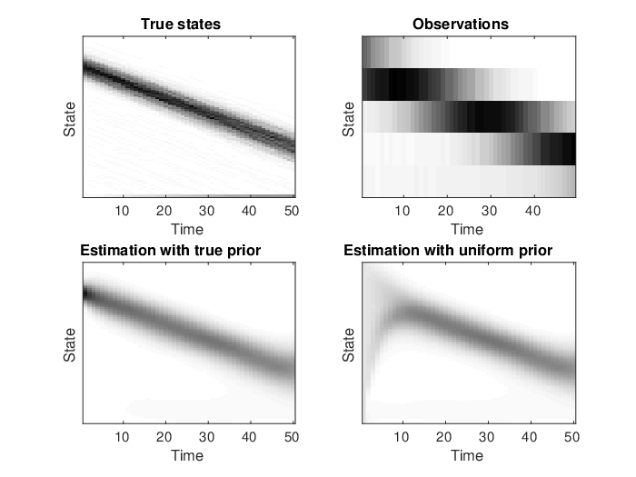
Consider a cloud of 1000 particles evolving from an initial distribution $\mu_{0}\in{\mathbb{R}}^{n}$ with $n=100$ states. The particles transition matrix is given by $\tilde{A}\in{\mathbb{R}}^{n\times n}$ with elements

$$\tilde{a}_{ij}\sim\exp\left(\frac{1}{2\sigma_{\tilde{a}}^{2}}(i-j-1)^{2}\right),\quad\mbox{ with }\sigma_{\tilde{a}}=0.5,$$

which corresponds to a discretization of a normal distribution ${\mathcal{N}}(1,0.5)$, and thus induces a drift on the dynamics of the cloud. The true dynamics of the particles are assumed to be unknown and instead modeled by a transition matrix $A\in{\mathbb{R}}^{n\times n}$ with elements

$$a_{ij}\sim\exp\left(\frac{1}{2\sigma_{a}^{2}}(i-j)^{2}\right),\quad\mbox{ with }\sigma_{a}=2.$$

At each time instance, the particles are observed in $m=5$ bins, where the observation probability matrix $B\in{\mathbb{R}}^{n\times m}$ has elements

$$b_{ij}\sim\exp\left(\frac{1}{2\sigma_{b}^{2}}\left(j-\frac{i+10}{20}\right)^{2}\right),\quad\mbox{ with }\sigma_{b}=0.5.$$

We estimate the flow of the particles and hidden particle distributions solving problem (10) for $T=50$ time instances with the method proposed in Proposition 2. One estimate is formed using the true initial distribution $\mu_{0}$ as a prior distribution, and for a second estimate we use a uniform prior.

Figure 2 shows the true hidden particle cloud, the corresponding observations, and the two estimates. With full information of the initial states available, the proposed method provides a good estimate of the hidden states despite discrepancies between the true and assumed transition matrices $\tilde{A}$ and $A$. In the case of no prior information, i.e., the prior distribution is set to be uniform, we see that the estimate converges to the estimate with true prior within a few time steps. This indicates that the proposed method is robust to modeling uncertainties and lack of information in the initial state.

In this example we consider the problem of tracking a number of indistinguishable agents over a network given measurements from sensors that are distributed around the network. This is inspired by [13], where an HMM is used to estimate the flow of a crowd in an urban environment based on observations generated when cell phones connect to Wi-Fi sensors. The environment is modeled as a network of nodes and arcs, where the arcs represent walking paths in the area and the nodes are the intersections between the paths.

For this application, the optimization problem (10) needs to be extended to allow for multiple measurements. To this end, let $\Phi_{st}$ be a set of observations from measurement unit $s$ at time point $t$, for $t=1,\dots,T$, and for $s=1,\dots,S$. We obtain the maximum likelihood solution as the optimal solution to¹¹ 1 This is a convex optimization problem which in principle can be solved with off-the-shelf solvers. In this example we use an efficient algorithm in the spirit of Proposition 2, but due to lack of space we defer the exact algorithm to a forthcoming paper.

	$\displaystyle\underset{M_{[1:T]},D_{[1:T],[1:S]},\mu_{[1:T]}}{\text{minimize }}\$	$\displaystyle\sum_{t=1}^{T}H(M_{t}\ |\ {\rm diag}(\mu_{t-1})A)$
		$\displaystyle+\sum_{t=1}^{T}\sum_{s=1}^{S}H(D_{st}\ |\ {\rm diag}(\mu_{t})B_{s})$
	subject to	$\displaystyle M_{t}{\bf 1}=\mu_{t-1},\quad M_{t}^{T}{\bf 1}=\mu_{t}$		(11)
		$\displaystyle D_{st}{\bf 1}=\mu_{t},\qquad D_{st}^{T}{\bf 1}=\Phi_{st}$
		$\displaystyle\text{for }t=1,\dots,T,\text{ and }s=1,\dots,S.$

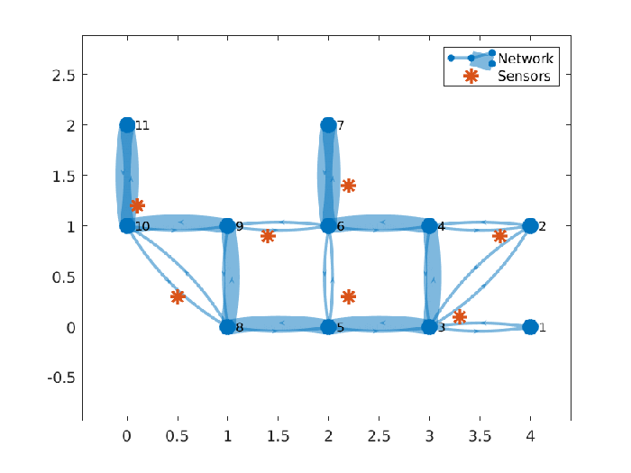
Consider a hidden Markov model where the states $X=\{X_{1},\ldots,X_{n}\}$ are the edges in the directed graph $\mathcal{G}=(V,X)$, and where the edge $X_{i}=(V^{\rm in}_{i},V^{\rm out}_{i})$ goes from $V^{\rm in}_{i}\in V$ to $V^{\rm out}_{i}\in V$. In this example we will use the graph illustrated in Figure 3, consisting of 11 nodes and $n=28$ edges. For the true model, transition probabilities are defined according to weights in the graph that represent which walking paths are preferred by the pedestrians. For the model used in the estimation we assume that this information is not known and use uniform weights. More specifically, the transition probabilities are given by

$$\tilde{a}_{ij}=\!\begin{cases}0.5,&\text{ if }j=i\\ \displaystyle{0.5\,w_{ij}\!\left(\sum_{\{k:V^{\rm in}_{k}=V^{\rm out}_{i}\}}w_{ik}\right)^{-1}}&\text{ if }V^{\rm in}_{j}=V^{\rm out}_{i}\\ 0,&\text{ else,}\end{cases}$$

where $\{w_{ij}\}$ is a set of weights. For the transition matrix $A$ used in the estimation we assign uniform weights $w_{ij}=1$, for all $(i,j)$ with $V^{\rm in}_{j}=V_{i}^{\rm out}$. For the true transitions the weights are defined as

$$w_{ij}=\begin{cases}20,&X_{j}\in\mathcal{W}$ and $V_{j}^{\rm out}\neq V_{i}^{\rm in}\\ 0,&V_{j}^{\rm out}=V_{i}^{\rm in}\\ 1,&\text{ else,}\end{cases}$$

for $(i,j)$ such that $V^{\rm in}_{j}=V_{i}^{\rm out}$, and where $\mathcal{W}$ is the set of edges highlighted in Figure 3. Note that the second case implies that agents do not transition to the reverse edge in the next time step.

The agents are observed by a set of $S=7$ sensors located at the positions indicated in Figure 3. The observation probability for an agent on edge $X_{i}$ to be detected by a given sensor $s$ is defined as $b^{s}_{i1}=\min(0.99,2e^{-5d})$, where $d$ denotes the Euclidean distance between the location of $s$ and the midpoint of $X_{i}$. Consequently the probability of not being detected is $b^{s}_{i2}=1-b^{s}_{i1}$.

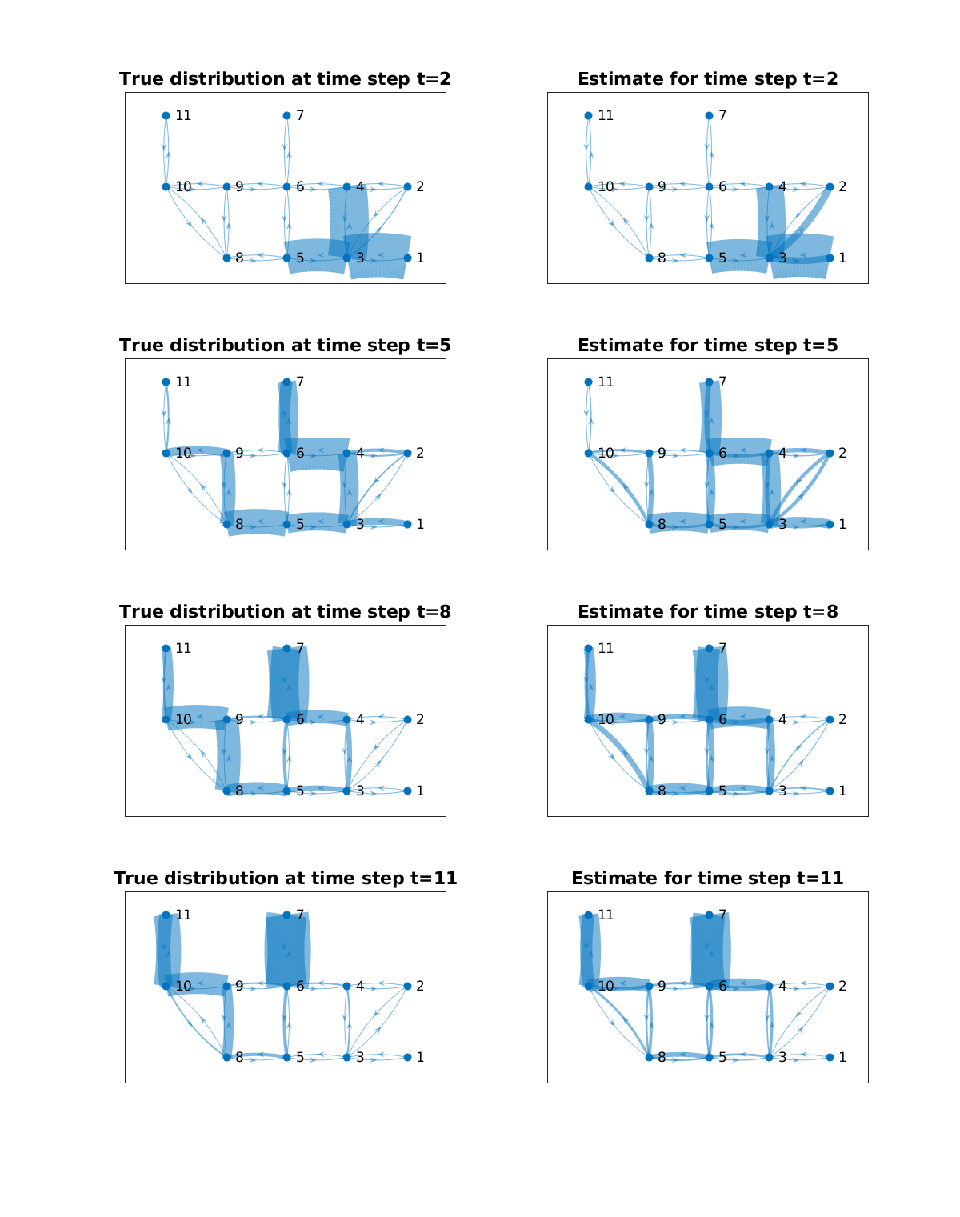
Given an initial distribution of 100 agents on the edge $(1,3)$, the flow and the measurements for the true ensemble are computed for $T=20$ time steps using the true transition and observation probabilities. Then we estimate the flow by solving the optimization problem (11). The true and estimated particle distributions are compared for some time steps in Figure 4, where the width of each edge is proportional to the number of agents on it. As can be seen in the figure the proposed method provides a good estimate also for this example.

Let $\mu_{0}^{(N)}$ and $M^{(N)}$ be as described in the statement of the proposition. Moreover, let $\mathcal{Z}^{(N)}=\{(i,j)\mid m^{(N)}_{ij}\neq 0\}$, which is non-empty, and let $\mathcal{Z}^{(N)}_{i}=\{j\mid(i,j)\in\mathcal{Z}^{(N)}\}$, which is non-empty if and only if $(\mu_{0}^{(N)})_{i}>0$. Furthermore, let $\mathcal{Y}^{(N)}=\{i\mid(\mu_{0}^{(N)})_{i}>0\}$. Then, using Stirling’s formula

$$\sqrt{2\pi}n^{n-1/2}e^{-n}\leq n!\leq en^{n-1/2}e^{-n},$$

see, e.g., [30], for $i\in\mathcal{Y}^{(N)}$ the multinomial coefficient in (4) can be bounded from above by

		$\displaystyle\binom{(\mu_{0}^{(N)})_{i}}{m_{i1}^{(N)},m_{i2}^{(N)},\dots,m_{in}^{(N)}}$
		$\displaystyle\leq e^{-(|\mathcal{Z}^{(N)}_{i}|-1)}\exp\bigg(\sum_{j\in\mathcal{Z}^{(N)}_{i}}m_{ij}^{(N)}-(\mu_{0}^{(N)})_{i}\bigg)$
		$\displaystyle\hskip 20.0pt\cdot(\mu_{0}^{(N)})_{i}^{(\mu_{0}^{(N)})_{i}+\frac{1}{2}}\prod_{j\in\mathcal{Z}^{(N)}_{i}}(m_{ij}^{(N)})^{-(m_{ij}^{(N)}+\frac{1}{2})}$
		$\displaystyle\leq(\mu_{0}^{(N)})_{i}^{(\mu_{0}^{(N)})_{i}+\frac{1}{2}}\prod_{j\in\mathcal{Z}^{(N)}_{i}}(m_{ij}^{(N)})^{-(m_{ij}^{(N)}+\frac{1}{2})},$

where $|\mathcal{Z}^{(N)}_{i}|$ denotes the cardinality of the set, and where the second inequality follows from the fact that $\sum_{j\in\mathcal{Z}^{(N)}_{i}}m_{ij}=\sum_{j=1}^{n}m_{ij}=(\mu_{0})_{i}$, and that $e^{-(|\mathcal{Z}^{(N)}_{i}|-1)}\leq 1$. Thus, the log-likelihood of the probability for a transfer plan $M^{(N)}$ can be upper-bounded as follows:

		$\displaystyle\log\left(P_{\mu_{0}^{(N)},A}(M^{(N)})\right)$
		$\displaystyle\leq\sum_{(i,j)\in\mathcal{Z}^{(N)}}\left(m_{ij}^{(N)}\log(a_{ij})-\left(m_{ij}^{(N)}+\frac{1}{2}\right)\log(m_{ij}^{(N)})\right)$
		$\displaystyle\quad+\sum_{i\in\mathcal{Y}^{(N)}}\left((\mu_{0}^{(N)})_{i}+\frac{1}{2}\right)\log((\mu_{0}^{(N)})_{i})$
		$\displaystyle=\sum_{(i,j)\in\mathcal{Z}^{(N)}}\left(m_{ij}^{(N)}\log\left(\frac{(\mu_{0}^{(N)})_{i}a_{ij}}{m_{ij}^{(N)}}\right)\right)$
		$\displaystyle\quad-\sum_{(i,j)\in\mathcal{Z}^{(N)}}\frac{1}{2}\log(m_{ij}^{(N)})+\sum_{i\in\mathcal{Y}^{(N)}}\frac{1}{2}\log((\mu_{0}^{(N)})_{i})$
		$\displaystyle\leq-H\left(M^{(N)},{\rm diag}(\mu_{0}^{(N)})A\right)+\frac{n}{2}\log(N),$

where the last inequality comes from the second-to-last expression by i) identifying the first term as the KL divergence, ii) noting that the second term is nonpositive, and iii) overestimating the third term by taking $(\mu_{0}^{(N)})_{i}=N$ for $i=1,\ldots,n$.

Similarly, underestimating the multinomial coefficients gives that the log-likelihood can be bounded from below by

		$\displaystyle\log\left(P_{\mu_{0}^{(N)},A}(M^{(N)})\right)$
		$\displaystyle\geq\sum_{(i,j)\in\mathcal{Z}^{(N)}}\left(m_{ij}^{(N)}\log\left(\frac{(\mu_{0}^{(N)})_{i}a_{ij}}{m_{ij}^{(N)}}\right)-\frac{1}{2}\log(m_{ij}^{(N)})\right)$
		$\displaystyle\quad+\sum_{i\in\mathcal{Y}^{(N)}}\frac{1}{2}\log((\mu_{0}^{(N)})_{i})-\frac{1}{2}n(n-1)\log(2\pi)$
		$\displaystyle\geq-H\left(M^{(N)},{\rm diag}(\mu_{0}^{(N)})A\right)$
		$\displaystyle\phantom{\geq}-\frac{1}{2}\left(n^{2}+\frac{n(n-1)\log(2\pi)}{\log(N)}\right)\log(N).$

By using the two inequalities, the result follows.

We solve (10) by a block coordinate ascent in the dual. First note that since $\mu_{0}$, $A$, $B$, and $\Phi_{t}$ are all elementwise nonnegative, so will the optimal solution $M_{[1:T]}^{*},D_{[1:T]}^{*},\mu_{[1:T]}^{*}$ also be. We can therefore add the constraint $\mu_{[1:T]}\geq 0$ to (10) without changing the optimal solution. For this problem, we relax the constraints in (10) with corresponding dual variables $\lambda_{M_{t}},\nu_{M_{t}},\lambda_{D_{t}},\nu_{D_{t}}$. Let $\mathfrak{M}:=M_{[1:T]}$, $\mathfrak{D}:=D_{[1:T]}$, and define the Lagrangian

		$\displaystyle L(\mathfrak{M},\mathfrak{D},\mu_{[1:T]},\lambda_{\mathfrak{M}},\nu_{\mathfrak{M}},\lambda_{\mathfrak{D}},\nu_{\mathfrak{D}})$
		$\displaystyle=\sum_{t=1}^{T}\Bigg(\sum_{ij}m^{t}_{ij}\log\big(\frac{m^{t}_{ij}}{\mu^{t-1}_{i}a_{ij}}\big)+\lambda_{M_{t}}^{T}(\mu_{t-1}-M_{t}{\bf 1})$
		$\displaystyle+\nu_{M_{t}}(\mu_{t}-M_{t}^{T}{\bf 1})+\sum_{ij}d^{t}_{ij}\log\big(\frac{d^{t}_{ij}}{\mu^{t}_{i}b_{ij}}\big)$
		$\displaystyle+\lambda_{D_{t}}^{T}(\mu_{t}-D_{t}{\bf 1})+\nu_{D_{t}}(\Phi_{t}-D_{t}^{T}{\bf 1})\Bigg).$

Minimizing this with respect to the matrices $M_{t}$ and $D_{t}$ gives explicit expressions for the optimal solution in terms of $\mu_{[0:T]}$ and the dual variables, i.e.,

	$\displaystyle M_{t}$	$\displaystyle=\frac{1}{e}{\rm diag}(\mu_{t-1}\odot u_{t})\,A\,{\rm diag}(w_{t}),$
	$\displaystyle D_{t}$	$\displaystyle=\frac{1}{e}{\rm diag}(\mu_{t}\odot x_{t})\,B\,{\rm diag}(v_{t}),$

where $u_{t}=\exp(\lambda_{M_{t}})$, $w_{t}=\exp(\nu_{M_{t}})$, $x_{t}=\exp(\lambda_{D_{t}})$ and $v_{t}=\exp(\nu_{D_{t}})$, for $t=1,\dots,T$. Plugging these into the Lagrangian, we get the modified Lagrangian

		$\displaystyle L(\mu_{[1:T]},u_{\mathfrak{M}},w_{\mathfrak{M}},x_{\mathfrak{D}},v_{\mathfrak{D}})=-\frac{1}{e}\sum_{t=1}^{T}(\mu_{t-1}\odot u_{t})^{T}Aw_{t}$
		$\displaystyle-\frac{1}{e}\sum_{t=1}^{T}(\mu_{t}\odot x_{t})^{T}Bv_{t}+\log(u_{1})^{T}\mu_{0}$
		$\displaystyle+\sum_{t=1}^{T-1}\mu_{t}^{T}\left(\log(u_{t+1})+\log(w_{t})+\log(x_{t})\right)$
		$\displaystyle+\mu_{T}^{T}(\log(w_{T})+\log(x_{T}))+\sum_{t=1}^{T}\log(v_{t})^{T}\Phi_{t}.$

Noting that since $\mu_{[1:T]}$ occurs linearly in $L$, for the modified dual functional $\inf_{\mu_{[1:T]}\geq 0}L(\mu_{[1:T]},\lambda_{\mathfrak{M}},\nu_{\mathfrak{M}},\lambda_{\mathfrak{D}},\nu_{\mathfrak{D}})$ to be bounded from below, the corresponding factors need to be elementwise nonnegative. In this case the corresponding terms will be zero when taking the infimum, and thus the dual problem is to maximize

$$-\frac{1}{e}(\mu_{0}\odot u_{1})^{T}Aw_{1}+\log(u_{1})^{T}\mu_{0}+\sum_{t=1}^{T}\log(v_{t})^{T}\Phi_{t}$$

(12)

subject to

$$\begin{split}-\frac{1}{e}{\rm diag}(u_{t+1})Aw_{t+1}-\frac{1}{e}{\rm diag}(x_{t})Bv_{t}&\\ +\log(u_{t+1})+\log(x_{t})+\log(w_{t})&\geq 0\end{split}$$

(13)

for $t=1,\dots,T-1$, and

$$-\frac{1}{e}{\rm diag}(x_{T})Bv_{T}+\log(x_{T})+\log(w_{T})\geq 0.$$

(14)

Note that neither the objective function (12), nor the first $T-1$ constraints (13) depend on $x_{T}$. Thus the optimal choice of $x_{T}$ is the one creating the most slack in the last constraint, i.e., the one maximizing the first two terms of (14). This is achieved by $x_{T}=e{\bf 1}./(Bv_{T})$, and for this choice of $x_{T}$ the constraint (14) can be replaced by

$$-\log(Bv_{T})+\log(w_{T})\geq 0.$$

(15)

Similarly, the slack in (13) is maximized by selecting

		$\displaystyle x_{t}=e{\bf 1}./\left(Bv_{t}\right),\quad t=1,\dots,T$
		$\displaystyle u_{t}=e{\bf 1}./\left(Aw_{t}\right),\quad t=2,\dots,T.$

and thus the constraints (13) can be replaced by

$$-\log(Aw_{t+1})-\log(Bv_{t})+\log(w_{t})\geq 0,$$

(16)

for $t=1,\ldots,T-1$. Next, note that if some of the constraints (15) and (16) are not fulfilled with equality, the objective function (12) can be improved by increasing the values of the corresponding $v_{t}$. Therefore, in an optimal point we must have that

	$\displaystyle w_{T}$	$\displaystyle=Bv_{T}$
	$\displaystyle w_{t}$	$\displaystyle=\left(Bv_{t}\right)\odot(Aw_{t+1})\quad\text{for }t=T-1,\dots,1.$

This gives an expression for $w_{1}$, that depends on $v_{t}$, $t=1,\ldots,T$. Inserting this into the objective (12) leads to an unconstrained problem that depends only on $u_{1}$ and $v_{t}$, $t=1,\dots,T$, which we solve using block coordinate ascent. To this end, the unconstrained objective is first maximized with respect to $u_{1}$, which gives

$$u_{1}=e{\bf 1}./(Aw_{1}).$$

Further, note that the gradient of the unconstrained objective with respect to $v_{t}$ is

$$-\frac{1}{e}\odot\left(B^{T}(y_{t}\odot Aw_{t+1})\right)+\Phi_{t}./v_{t},$$

where $y_{t}$ is defined by the recursion

	$\displaystyle y_{1}$	$\displaystyle=A^{T}(\mu_{0}\odot u_{1}),$
	$\displaystyle y_{t}$	$\displaystyle=A^{T}(y_{t-1}\odot(Bv_{t-1})),\quad t=2,\dots,T.$

Hence, maximization with respect to $v_{t}$ is achieved by

$$v_{t}=e\Phi_{t}./\left(B^{T}(y_{t}\odot Aw_{t+1})\right).$$

As the unconstrained problem is convex and the objective function continuously differentiable, the block coordinate ascent method converges [3, Prop. 2.7.1]. In the limit point, the hidden marginals can be reconstructed from

	$\displaystyle\mu_{t}=M_{t}^{T}{\bf 1}$	$\displaystyle=\frac{1}{e}{\rm diag}(w_{t})A^{T}(\mu_{t-1}\odot u_{t})$
		$\displaystyle={\rm diag}(w_{t})A^{T}(\mu_{t-1}./(Aw_{t})).$

References

- [1] J.-D. Benamou, G. Carlier, M. Cuturi, L. Nenna, and G. Peyré. Iterative bregman projections for regularized transportation problems. SIAM Journal on Scientific Computing, 37(2):A1111–A1138, 2015.
- [2] G. Bernstein and D. Sheldon. Consistently estimating Markov chains with noisy aggregate data. In Proceedings of the 19th International Conference on Artificial Intelligence and Statistics, pages 1142–1150. Society for Artificial Intelligence and Statistics, 2016.
- [3] D.P. Bertsekas. Nonlinear Programming. Athena Scientific, 1999.
- [4] S. Blackman and R. Popoli. Design and analysis of modern tracking systems. Artech House, Norwood, MA, 1999.
- [5] F. Carravetta and L.B. White. Modelling and estimation for finite state reciprocal processes. IEEE Transactions on Automatic Control, 57(9):2190–2202, 2012.
- [6] Y. Chen, G. Conforti, and T. T. Georgiou. Measure-valued spline curves: An optimal transport viewpoint. SIAM Journal on Mathematical Analysis, 50(6):5947–5968, 2018.
- [7] Y. Chen, T. Georgiou, and M. Pavon. Entropic and displacement interpolation: A computational approach using the Hilbert metric. SIAM Journal on Applied Mathematics, 76(6):2375–2396, 2016.
- [8] Y. Chen, T. Georgiou, M. Pavon, and A. Tannenbaum. Robust transport over networks. IEEE Transactions on Automatic Control, 62(9):4675–4682, 2017.
- [9] Y. Chen, T.T. Georgiou, and M. Pavon. On the relation between optimal transport and Schrödinger bridges: A stochastic control viewpoint. Journal of Optimization Theory and Applications, 169(2):671–691, 2016.
- [10] Y. Chen and J. Karlsson. State tracking of linear ensembles via optimal mass transport. IEEE Control Systems Letters, 2(2):260–265, 2018.
- [11] T.M. Cover and J.A. Thomas. Elements of information theory. John Wiley & Sons, Hoboken, NJ, 2006.
- [12] M. Cuturi. Sinkhorn distances: Lightspeed computation of optimal transport. In Advances in Neural Information Processing Systems (NIPS), pages 2292–2300. Neural Information Processing Systems Foundation, 2013.
- [13] S. Danielsson and J. Flygare. A multi-target graph-constrained HMM localisation approach using sparse wi-fi sensor data. Master thesis, KTH Royal Institute of Technology, 2018.
- [14] D. Dawson, L. Gorostiza, and A. Wakolbinger. Schrödinger processes and large deviations. Journal of mathematical physics, 31(10):2385–2388, 1990.
- [15] A. Dembo and O. Zeitouni. Large deviations techniques and applications. Springer-Verlag Berlin Heidelberg, 2009.
- [16] R. Ellis. Entropy, Large Deviations, and Statistical Mechanics. Springer-Verlag Berlin Heidelberg, 2006.
- [17] F. Elvander, I. Haasler, A. Jakobsson, and J. Karlsson. Tracking and sensor fusion in direction of arrival estimation using optimal mass transport. In 2018 26th European Signal Processing Conference (EUSIPCO), pages 1617–1621. IEEE, 2018.
- [18] M. Fanaswala, V. Krishnamurthy, and L.B. White. Destination-aware target tracking via syntactic signal processing. In 2011 IEEE International Conference on Acoustics, Speech and Signal Processing (ICASSP), pages 3692–3695, 2011.
- [19] H. Föllmer. Random fields and diffusion processes. In P.-L. Hennequin, editor, École d’Été de Probabilités de Saint-Flour XV–XVII, 1985–87, volume 1362 of Lecture Notes in Mathematics, pages 101–203. Springer, Berlin, Heidelberg, 1988.
- [20] T.T. Georgiou and M. Pavon. Positive contraction mappings for classical and quantum Schrödinger systems. Journal of Mathematical Physics, 56(3):033301, 2015.
- [21] Z. Ghahramani. An introduction to hidden Markov models and Bayesian networks. International journal of pattern recognition and artificial intelligence, 15(1):9–42, 2001.
- [22] B. Jamison. Reciprocal processes. Probability Theory and Related Fields, 30(1):65–86, 1974.
- [23] J. Karlsson and A. Ringh. Generalized Sinkhorn iterations for regularizing inverse problems using optimal mass transport. SIAM Journal on Imaging Sciences 10(4), 1935–1962, 2017.
- [24] G. King. A Solution to the Ecological Inference Problem: Reconstructing Individual Behavior from Aggregate Data. Princeton University Press, Princeton, NJ, 1997.
- [25] B.C. Levy, R. Frezza, and A.J. Krener. Modeling and estimation of discrete-time gaussian reciprocal processes. IEEE Transactions on Automatic Control, 35(9):1013–1023, 1990.
- [26] C. Léonard. A survey of the Schrödinger problem and some of its connections with optimal transport. Discrete & Continuous Dynamical Systems - A, 34(4):1533–1574, 2014.
- [27] T. Mikami. Monge’s problem with a quadratic cost by the zero-noise limit of -path processes. Probability Theory and Related Fields, 129(2):245–260, 2004.
- [28] M. Pavon and F. Ticozzi. Discrete-time classical and quantum Markovian evolutions: Maximum entropy problems on path space. Journal of Mathematical Physics, 51(4):042104, 2010.
- [29] L.R. Rabiner. A tutorial on hidden Markov models and selected applications in speech recognition. Proceedings of the IEEE, 77(2):257–286, 1989.
- [30] H. Robbins. A remark on Stirling’s formula. The American Mathematical Monthly, 62(1):26–29, 1955.
- [31] E. Schrödinger. Über die Umkehrung der Naturgesetze. Sitzungsberichte der Preussischen Akademie der Wissenschaften, Physikalisch-mathematische Klasse, pages 144–153, 1931.
- [32] G. Stamatescu, L.B. White, and R. Bruce-Doust. Track extraction with hidden reciprocal chains. IEEE Transactions on Automatic Control, 63(4):1097–1104, 2018.
- [33] C. Villani. Optimal transport: Old and new. Springer, Berlin Heidelberg, 2008.
- [34] L.B. White and H.X. Vu. Maximum likelihood sequence estimation for hidden reciprocal processes. IEEE Transactions on Automatic Control, 58(10):2670–2674, 2013.
- [35] S. Zeng, S. Waldherr, C. Ebenbauer, and F. Allgöwer. Ensemble observability of linear systems. IEEE Transactions on Automatic Control, 61(6):1452–1465, 2016.