Correlating Tauonic B Decays to the Neutron EDM via a Scalar LeptoquarkPreprint: PSI-PR-19-08, ZU-TH 25/19
Abstract
In this article we investigate the correlations between tauonic meson decays (e.g. , , ) and electric dipole moments (EDMs), in particular the one of the neutron, in the context of the scalar leptoquark. We perform the matching of this model on the effective field theory taking into account the leading renormalization group effect for the relevant observables. We find that one can explain the hints for new physics in transitions without violating bounds from other observables. Even more interesting, it can also give sizable effects in , to be tested at BELLE II, which are correlated to (chromo) electric dipole operators receiving enhanced contributions. Therefore, given a deviation from the Standard Model (SM) expectations in , this model predicts a sizable neutron EDM. In fact, even if new physics has CP conserving real couplings, the CKM matrix induces a complex phase and already a 10% change of the branching ratio (with respect to the SM) will lead to an effect observable with the n2EDM experiment at PSI.
I Introduction
In the past four decades, the Standard Model (SM) of particle physics has been extensively tested and its predictions were very successfully confirmed, both in high energy searches as well as in low energy precision experiments. However, it is well known that the SM cannot be the ultimate theory describing the fundamental constituents of matter and their interactions. For example, it cannot accommodate for the observed matter–antimatter asymmetry in the universe: For satisfying the Sakharov conditions Sakharov 1967 the amount of CP violation within the SM is far too small Cohen et al. 1993; Gavela et al. 1994a; Huet and Sather 1995; Gavela et al. 1994b; Gavela et al. 1994c; Riotto and Trodden 1999. Therefore, additional sources of CP violation are required and such models in general lead to nonvanishing electric dipole moments of neutral fermions. Thus, EDMs are very promising places to search for physics beyond the SM (see e.g. Ref. Chupp et al. 2019; Yamanaka et al. 2017 for a recent review). However, the effect of new physics (NP) in EDMs decouples with the NP scale which is a priori unknown, unless new particles, or at least deviations from the SM in other precision observables, are found.
In this respect, tauonic decays are very promising channels for the (indirect) search for NP, especially in the light of the observed tensions between the SM predictions and experiments above the 3 level Amhis et al. 2017. These decays involve both down-type quarks and charged leptons of the third generation (i.e. bottom quarks and tau leptons) which are, due to their mass, very special and distinct from the fermions of the first two generations.11 1 In group theory language, the SM possesses a global flavor symmetry which is broken by the thrid generation Yukawa couplings to Barbieri et al. 1996. In fact, to explain these anomalies, TeV scale NP with order one couplings to the third generation is required. Note that the tensions in transitions are supported by data (i.e. and ) and the forthcoming measurements of both and processes by LHCb and BELLE II will be able to confirm (or disprove) the presence of NP in these decays.
Therefore, it is very interesting to investigate the possible impact of models which can give sizable effects in tauonic decays and EDMs. In this paper we choose the scalar leptoquark singlet which couples to SM fermions via the Lagrangian
| (1) |
Here, () is the lepton (charge conjugated quark) doublet, () the charged lepton (charge conjugated up quark) singlet and are flavor indices. This model is theoretically well motivated since is present within the -parity violating MSSM in the form of right-handed down squarks Hall and Suzuki 1984; Ross and Valle 1985; Barger et al. 1989; Dreiner 1997; Barbier et al. 2005.22 2 Note that in the minimal R-parity violating MSSM the coupling to charged conjugated fields in Eq. (1) is absent. For an analysis of EDM constraints within this setup see Ref. Yamanaka et al. 2014.
This leptoquark (LQ) is a prime candidate for providing the desired correlations between tauonic decays and EDMs. It possesses couplings to left- and right-handed quarks which is a necessary requirement for generating EDMs at the one-loop level Fuyuto et al. 2019; Dekens et al. 2019. It also contributes to at tree level Fajfer et al. 2012; Deshpande and Menon 2013; Tanaka and Watanabe 2013; Sakaki et al. 2013; Freytsis et al. 2015; Hati et al. 2016; Bauer and Neubert 2016; Li et al. 2016; Zhu et al. 2016; Popov and White 2017; Deshpande and He 2017; Crivellin et al. 2017a; Altmannshofer et al. 2017; Kamali et al. 2018; Azatov et al. 2018; Zhu et al. 2018; Hu et al. 2019; Angelescu et al. 2018; Kim et al. 2018; Yan et al. 2019 and gives a very good fit to data (including polarization observables) Feruglio et al. 2018; Iguro et al. 2019; Blanke et al. 2019; Murgui et al. 2019 since it generates vector, scalar and tensor operators. Similarly, it contributes to transitions, in particular to , where the situation becomes especially interesting. As we will see, in this case the model leads to enhanced CP violating effects in (chromo) electric dipole operators (see Fig. 1) which are even present for real NP parameters due to the large phase contained in the CKM element .
II Observables and Contributions
In this section we discuss our setup, calculate the predictions for the relevant observables and discuss their current experimental situation and future prospects.
After electroweak symmetry breaking, the Lagrangian in Eq. (1) decomposes into components
Here, we work in the down basis, meaning that the CKM matrix appears in the couplings to left-handed up-type quarks. We denote the mass of the LQ by and neglect its couplings to the SM Higgs boson which have a negligible phenomenological impact. The most relevant classes of observables in our model are and transitions as well as EDMs, mixing and - as well as - couplings which we consider now in more detail.
II.1
For transitions we follow the conventions of Ref. Buras et al. 2015
| (2) |
and obtain, already at tree level, the contribution
| (3) |
Here the most relevant decays are for which and branching ratios, normalized by the corresponding SM predictions, read
| (4) |
This has to be compared to the current experimental limits and Grygier et al. 2017 (both at ). The future BELLE II sensitivity for is 30% of the SM branching ratio Abe et al. 2010.
II.2
For tauonic decays we define the effective Hamiltonian as
with the operators given by
| (5) |
In the SM and our NP matching contributions at tree level are given by
| (6) |
Taking into account the QCD effects of Ref. Aebischer et al. 2019 to the matching, the one-loop EW and two-loop QCD renormalization group equation (RGE) for the scalar and tensor operators Gracey 2000; González-Alonso et al. 2017 can be taken consistently into account. Numerically, this RGE evolution is given by
for a matching scale of . Finally, the, ratios with in terms of the Wilson coefficients at the scale are given by Blanke et al. 2019
| (13) |
Similarly, for transitions we have
| (14) |
The corresponding formula for can be found in Ref. Tanaka and Watanabe 2017. However, here the effect of scalar and tensor operators is much smaller, making the theoretically very clean decays the primary place to search for them.
Combining the experimental measurements of transitions from LHCb Aaij et al. 2015; Aaij et al. 2018a; Aaij et al. 2018b, Belle Huschle et al. 2015; Sato et al. 2016; Hirose et al. 2017; Hirose et al. 2018; Abdesselam et al. 2019 and Babar Lees et al. 2012; Lees et al. 2013, one finds a combined tension of in Amhis et al. 201733 3 In Ref. Ikeno et al. 2019 it was shown that uncertainties from meson exchanges between initial and final states might be bigger than the estimated SM uncertainty, which could alleviate the tension in . On the other hand, recent improvements in form factor calculations Bordone et al. 2019 lower the SM prediction and increase the tension. These two effects are not included in Ref. Amhis et al. 2017 but will not change the result significantly.. However, note that here the measurement of LHCb Aaij et al. 2018c, which also lies significantly above the SM prediction, is not included.44 4 See Ref. Watanabe 2018; Chauhan and Kindra 2017 for an analysis including before the latest BELLE update Abdesselam et al. 2019. In transitions, the theory prediction for crucially depends on . While previous lattice calculations resulted in rather small values of , recent calculations give a larger value (see Ref. Ricciardi 2017 for an overview). However, the measurement is still above the SM prediction by more than 1, as can be seen from the global fit Charles et al. 2005. In there is also a small disagreement between theory Bernlochner 2015 and experiment Hamer et al. 2016 which does not depend on , once more pointing towards an enhancement. Therefore, even though the results are not significant on their own, they point in the same direction as (i.e. towards an enhancement with respect to the SM) and thus strengthen the case for NP in tauonic decays.
II.3 EDMs
For EDMs the relevant Hamiltonian in our case is
| (15) |
with
| (16) |
At the high scale we find the matching contributions (depicted in Fig. 1)
| (17) |
Note that we only get up-quark contributions since we do not have (at the one-loop level) CP violating couplings to down-type quarks. Importantly, note that our effect in and is parametrically enhanced by , making a sizable effect in EDMs possible. This enhancement of the dipole operators also allows us to safely neglect the effects of charm quarks, four-fermion operators and of the Weinberg operator otherwise relevant for LQs Dekens et al. 2019.
Next, we use the one-loop RGE to evolve these Wilson coefficients of Eq. (17) down to the neutron scale. Here, combining and adjusting the results of Ref. Crivellin et al. 2017b and Ref. Borzumati and Greub 1998 to our case we obtain55 5 For the same RGE in a different operator basis see Ref. Hisano et al. 2012.
The solution to this differential equation can be written in terms of an evolution matrix in the form
| (18) |
with
| (22) | ||||
| and | ||||
| (23) | ||||
where is the number of active quark flavors. The final evolution matrix is obtained by running with the appropriate numbers of flavours from the LQ scale down to 1 GeV.
Finally, the effects in the neutron and proton EDMs are given by Cirigliano et al. 2016
in terms of the Wilson coefficients evaluated at 1 GeV. The neutron and proton EDMs then enter atomic ones, most importantly in mercury and deuteron (see Ref. Cirigliano et al. 2016 for details).
On the experimental side, Graner et al. 2016 gives currently slightly better bounds than the neutron EDM, while the one of the proton and the deuteron is not measured yet. However, and will be very precisely known from future experiments Pretz 2013; Eversmann et al. 2015 and concerning there will be soon an improvement of one order of magnitude in sensitivity compared to the current limit of Baker et al. 2006; Pendlebury et al. 2015 from the n2EDM experiment at PSI Abel et al. 2018. Therefore, we will focus on in our phenomenological analysis.
 |
II.4 mixing
To describe mixing we use the effective Hamiltonian
and find at the high scale
| (24) |
from the one-loop matching. The evolution of was calculated in Refs. Buras et al. 2000; Ciuchini et al. 1998 and yields approximately Golowich et al. 2007
| (25) |
The matrix element for the -meson mixing is given by
| (26) |
where at the scale Carrasco et al. 2014. The mass difference in the -meson system is given by
| (27) |
Further, we write
| (28) |
The averages of the experimental values read Bevan et al. 2014; Bazavov et al. 2018
| (29) |
at 95% C.L. At a high luminosity LHC (HL-LHC) the sensitivity to could be improved down to the SM expectation of Cerri et al. 2018.
II.5 and
Virtual corrections with top quarks and LQs modify couplings of gauge bosons to charged leptons, in particular to the tau. Parametrizing the interactions as
with
the LQ effects at (the contributions proportional to gauge boson mass are suppressed) are given by
| (30) |
with and . This leads to . Experimentally, the averaged modification of the - coupling extracted from and decays reads (averaging the central value but with unchanged error) Pich 2014; Tanabashi et al. 2018
| (31) |
which provides a better constraint than data of decays.
Concerning the axial vector coupling is much better constrained that the vectorial onePich 2014; Tanabashi et al. 2018
| (32) |
with .
III Phenomenology
Looking at the phenomenological consequences of our model, note that couplings to muons or electrons are obviously not necessary to obtain the desired effects in tauonic decays. Even though our model can in principle account for the anomalous magnetic moment of the muon Djouadi et al. 1990; Davidson et al. 1994; Couture and Konig 1996; Chakraverty et al. 2001; Cheung 2001; Mahanta 2001; Queiroz et al. 2015; Bauer and Neubert 2016; Das et al. 2016; Biggio et al. 2016; Crivellin et al. 2018 (or electron Crivellin et al. 2018) via a enhanced effect, this is not possible in the presence of large couplings to tau leptons since also here enhanced effects generate too large rates of . Similarly, our model cannot address the anomalies if one aims at a sizable effect in tauonic decays Bečirević et al. 2016. Therefore, we will disregard (i.e. set to zero) the couplings to muons and electrons. Couplings to top-quarks affect Feruglio et al. 2017 and Arnan et al. 2019. Here we see that and (for TeV) is compatible with experiments for . Note that we improve the agreement in data while slightly worsening data, which is already a bit away from the SM prediction.
Thus, we are left with , and as free parameters for studying the effect in tauonic decays and the correlations with EDMs. In the following we will set TeV which is also well compatible with the latest direct search results of CMS for third generation LQs Takahashi 2019; Sirunyan et al. 2018.66 6 More sophisticated analysis of LHC data can be found in Refs. Raj 2017; Bansal et al. 2018; Mandal et al. 2019. However, since for t-channel exchange the EFT limits are in general stronger than the ones in the UV complete model, we will use for simplicity the results of Ref. Greljo et al. 2019 in the following which show that 1 TeV is compatible with data.
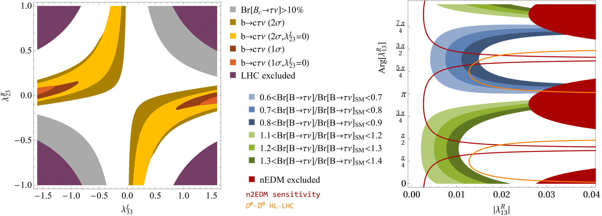
Let us now turn to processes, where effects of the order of 10% compared to the corresponding tree-level SM amplitude are required. Since our model can give (according to Eq. (3)) tree-level effects in decays (which are loop suppressed in the SM), these contributions must be suppressed. Since the bottom coupling to taus should be sizable, the coupling to strange quarks is tightly bound. We show the preferred regions, according to the updated global fit of Ref. Blanke et al. 2019, from processes in the left plot of Fig. 2. These regions are shown for but also the possible impact of , taking its maximally allowed values from , is depicted. Note that our model is not in conflict with the lifetime Celis et al. 2017; Alonso et al. 2017 (in fact, it is even compatible with the 10% limit of Ref. Akeroyd and Chen 2017) nor with direct LHC searches for monotaus Greljo et al. 2019. So far we worked with real parameters in order to maximize the effect in . However, even for complex couplings the effect in nuclear and atomic EDMs would be strongly suppressed since only up and down quarks contribute directly to these observables.
Therefore, let us now turn to where couplings to up quarks are obviously needed. Here, even for real couplings an effect in the neutron EDM is generated due to the large phase of . This effect could only be avoided for . However, since there is no (obvious) symmetry which could impose this relation, such a configuration would be fine-tuning. This can be seen from the right plot in Fig. 2, where we show the predictions for as a function of the absolute value and the phase of for (as preferred by data). The dark red contour lines denote the n2EDM sensitivity, showing that a 10% effect in with respect to the SM will lead to an observable effect in the neutron EDM within our model. Finally, taking , as preferred by (see left plot of Fig. 2), CP violation in mixing is generated. Here the red contour denotes the future HL-LHC sensitivity which is complementary to the region covered by EDM searches.
IV Conclusions
In this article we studied the interplay between tauonic meson decays and EDMs (in particular the one of the neutron) in a model with a scalar LQ singlet which can be identified with the right-handed down squark in the R-parity violating MSSM. We found that in order to explain the intriguing tensions in data, must be sizable and also a coupling to right-handed charm quarks and tau-leptons () is required. In this setup, the model gives a very good fit to data and is compatible with observables, LHC searches and lifetime constraints. Extending this analysis to transitions, in particular , again right-handed couplings to up quarks () are required to have a sizable effect. This leads to very important enhanced effects in (chromo) electric dipole operators generating in turn EDMs of nucleons and atoms. In particular, even for real couplings of the LQ to fermions, the large phase of generates a sizable contribution to the neutron EDM. In fact, this effect should already be observable in the n2EDM experiment at PSI, assuming that, within our model, is enhanced (or suppressed) by around 10% with respect to the SM.
Acknowledgments — The work of A.C. is supported by a Professorship Grant (PP00P2_176884) of the Swiss National Science Foundation. The work of F.S. is supported by the Swiss National Foundation under Grant No. 200020_175449/1. We thank Dario Müller for collaboration in the early stages of this article and Christoph Greub for useful comments on the manuscript. We are grateful to David Straub and Jason Aebischer for reminding us of the importance of - and - couplings.
References
- Sakharov (1967) A. D. Sakharov, Violation of CP Invariance, C asymmetry, and baryon asymmetry of the universe, Pisma Zh. Eksp. Teor. Fiz. 5, 32 (1967), [Usp. Fiz. Nauk161,no.5,61(1991)].
- Cohen et al. (1993) A. G. Cohen, D. B. Kaplan, and A. E. Nelson, Progress in electroweak baryogenesis, Ann. Rev. Nucl. Part. Sci. 43, 27 (1993), arXiv:hep-ph/9302210 [hep-ph] .
- Gavela et al. (1994a) M. B. Gavela, P. Hernandez, J. Orloff, and O. Pene, Standard model CP violation and baryon asymmetry, Mod. Phys. Lett. A9, 795 (1994a), arXiv:hep-ph/9312215 [hep-ph] .
- Huet and Sather (1995) P. Huet and E. Sather, Electroweak baryogenesis and standard model CP violation, Phys. Rev. D51, 379 (1995), arXiv:hep-ph/9404302 [hep-ph] .
- Gavela et al. (1994b) M. B. Gavela, M. Lozano, J. Orloff, and O. Pene, Standard model CP violation and baryon asymmetry. Part 1: Zero temperature, Nucl. Phys. B430, 345 (1994b), arXiv:hep-ph/9406288 [hep-ph] .
- Gavela et al. (1994c) M. B. Gavela, P. Hernandez, J. Orloff, O. Pene, and C. Quimbay, Standard model CP violation and baryon asymmetry. Part 2: Finite temperature, Nucl. Phys. B430, 382 (1994c), arXiv:hep-ph/9406289 [hep-ph] .
- Riotto and Trodden (1999) A. Riotto and M. Trodden, Recent progress in baryogenesis, Ann. Rev. Nucl. Part. Sci. 49, 35 (1999), arXiv:hep-ph/9901362 [hep-ph] .
- Chupp et al. (2019) T. Chupp, P. Fierlinger, M. Ramsey-Musolf, and J. Singh, Electric dipole moments of atoms, molecules, nuclei, and particles, Rev. Mod. Phys. 91, 015001 (2019), arXiv:1710.02504 [physics.atom-ph] .
- Yamanaka et al. (2017) N. Yamanaka, B. K. Sahoo, N. Yoshinaga, T. Sato, K. Asahi, and B. P. Das, Probing exotic phenomena at the interface of nuclear and particle physics with the electric dipole moments of diamagnetic atoms: A unique window to hadronic and semi-leptonic CP violation, Eur. Phys. J. A53, 54 (2017), arXiv:1703.01570 [hep-ph] .
- Amhis et al. (2017) Y. Amhis et al. (HFLAV), Averages of -hadron, -hadron, and -lepton properties as of summer 2016, Eur. Phys. J. C77, 895 (2017), arXiv:1612.07233 [hep-ex] .
- Barbieri et al. (1996) R. Barbieri, G. R. Dvali, and L. J. Hall, Predictions from a U(2) flavor symmetry in supersymmetric theories, Phys. Lett. B377, 76 (1996), arXiv:hep-ph/9512388 [hep-ph] .
- Hall and Suzuki (1984) L. J. Hall and M. Suzuki, Explicit R-Parity Breaking in Supersymmetric Models, Nucl. Phys. B231, 419 (1984).
- Ross and Valle (1985) G. G. Ross and J. W. F. Valle, Supersymmetric Models Without R-Parity, Phys. Lett. 151B, 375 (1985).
- Barger et al. (1989) V. D. Barger, G. F. Giudice, and T. Han, Some New Aspects of Supersymmetry R-Parity Violating Interactions, Phys. Rev. D40, 2987 (1989).
- Dreiner (1997) H. K. Dreiner, An Introduction to explicit R-parity violation, , 462 (1997), [Adv. Ser. Direct. High Energy Phys.21,565(2010)], arXiv:hep-ph/9707435 [hep-ph] .
- Barbier et al. (2005) R. Barbier et al., R-parity violating supersymmetry, Phys. Rept. 420, 1 (2005), arXiv:hep-ph/0406039 [hep-ph] .
- Yamanaka et al. (2014) N. Yamanaka, T. Sato, and T. Kubota, Linear programming analysis of the -parity violation within EDM-constraints, JHEP 12, 110, arXiv:1406.3713 [hep-ph] .
- Fuyuto et al. (2019) K. Fuyuto, M. Ramsey-Musolf, and T. Shen, Electric Dipole Moments from CP-Violating Scalar Leptoquark Interactions, Phys. Lett. B788, 52 (2019), arXiv:1804.01137 [hep-ph] .
- Dekens et al. (2019) W. Dekens, J. de Vries, M. Jung, and K. K. Vos, The phenomenology of electric dipole moments in models of scalar leptoquarks, JHEP 01, 069, arXiv:1809.09114 [hep-ph] .
- Fajfer et al. (2012) S. Fajfer, J. F. Kamenik, I. Nisandzic, and J. Zupan, Implications of Lepton Flavor Universality Violations in B Decays, Phys. Rev. Lett. 109, 161801 (2012), arXiv:1206.1872 [hep-ph] .
- Deshpande and Menon (2013) N. G. Deshpande and A. Menon, Hints of R-parity violation in B decays into , JHEP 01, 025, arXiv:1208.4134 [hep-ph] .
- Tanaka and Watanabe (2013) M. Tanaka and R. Watanabe, New physics in the weak interaction of , Phys. Rev. D87, 034028 (2013), arXiv:1212.1878 [hep-ph] .
- Sakaki et al. (2013) Y. Sakaki, M. Tanaka, A. Tayduganov, and R. Watanabe, Testing leptoquark models in , Phys. Rev. D88, 094012 (2013), arXiv:1309.0301 [hep-ph] .
- Freytsis et al. (2015) M. Freytsis, Z. Ligeti, and J. T. Ruderman, Flavor models for , Phys. Rev. D92, 054018 (2015), arXiv:1506.08896 [hep-ph] .
- Hati et al. (2016) C. Hati, G. Kumar, and N. Mahajan, excesses in ALRSM constrained from , decays and mixing, JHEP 01, 117, arXiv:1511.03290 [hep-ph] .
- Bauer and Neubert (2016) M. Bauer and M. Neubert, Minimal Leptoquark Explanation for the R , RK , and Anomalies, Phys. Rev. Lett. 116, 141802 (2016), arXiv:1511.01900 [hep-ph] .
- Li et al. (2016) X.-Q. Li, Y.-D. Yang, and X. Zhang, Revisiting the one leptoquark solution to the R(D(∗)) anomalies and its phenomenological implications, JHEP 08, 054, arXiv:1605.09308 [hep-ph] .
- Zhu et al. (2016) J. Zhu, H.-M. Gan, R.-M. Wang, Y.-Y. Fan, Q. Chang, and Y.-G. Xu, Probing the R-parity violating supersymmetric effects in the exclusive decays, Phys. Rev. D93, 094023 (2016), arXiv:1602.06491 [hep-ph] .
- Popov and White (2017) O. Popov and G. A. White, One Leptoquark to unify them? Neutrino masses and unification in the light of , and anomalies, Nucl. Phys. B923, 324 (2017), arXiv:1611.04566 [hep-ph] .
- Deshpande and He (2017) N. G. Deshpande and X.-G. He, Consequences of R-parity violating interactions for anomalies in and , Eur. Phys. J. C77, 134 (2017), arXiv:1608.04817 [hep-ph] .
- Crivellin et al. (2017a) A. Crivellin, D. Müller, and T. Ota, Simultaneous explanation of R(D(∗)) and : the last scalar leptoquarks standing, JHEP 09, 040, arXiv:1703.09226 [hep-ph] .
- Altmannshofer et al. (2017) W. Altmannshofer, P. S. Bhupal Dev, and A. Soni, anomaly: A possible hint for natural supersymmetry with -parity violation, Phys. Rev. D96, 095010 (2017), arXiv:1704.06659 [hep-ph] .
- Kamali et al. (2018) S. Kamali, A. Rashed, and A. Datta, New physics in inclusive decay in light of measurements, Phys. Rev. D97, 095034 (2018), arXiv:1801.08259 [hep-ph] .
- Azatov et al. (2018) A. Azatov, D. Bardhan, D. Ghosh, F. Sgarlata, and E. Venturini, Anatomy of anomalies, JHEP 11, 187, arXiv:1805.03209 [hep-ph] .
- Zhu et al. (2018) J. Zhu, B. Wei, J.-H. Sheng, R.-M. Wang, Y. Gao, and G.-R. Lu, Probing the R-parity violating supersymmetric effects in and decays, Nucl. Phys. B934, 380 (2018), arXiv:1801.00917 [hep-ph] .
- Hu et al. (2019) Q.-Y. Hu, X.-Q. Li, Y. Muramatsu, and Y.-D. Yang, R-parity violating solutions to the anomaly and their GUT-scale unifications, Phys. Rev. D99, 015008 (2019), arXiv:1808.01419 [hep-ph] .
- Angelescu et al. (2018) A. Angelescu, D. Bečirević, D. A. Faroughy, and O. Sumensari, Closing the window on single leptoquark solutions to the -physics anomalies, JHEP 10, 183, arXiv:1808.08179 [hep-ph] .
- Kim et al. (2018) T. J. Kim, P. Ko, J. Li, J. Park, and P. Wu, Correlation between and top quark FCNC decays in leptoquark models, (2018), arXiv:1812.08484 [hep-ph] .
- Yan et al. (2019) H. Yan, Y.-D. Yang, and X.-B. Yuan, Phenomenology of decays in a scalar leptoquark model, (2019), arXiv:1905.01795 [hep-ph] .
- Feruglio et al. (2018) F. Feruglio, P. Paradisi, and O. Sumensari, Implications of scalar and tensor explanations of , JHEP 11, 191, arXiv:1806.10155 [hep-ph] .
- Iguro et al. (2019) S. Iguro, T. Kitahara, Y. Omura, R. Watanabe, and K. Yamamoto, D∗ polarization vs. anomalies in the leptoquark models, JHEP 02, 194, arXiv:1811.08899 [hep-ph] .
- Blanke et al. (2019) M. Blanke, A. Crivellin, S. de Boer, M. Moscati, U. Nierste, I. Nišandžić, and T. Kitahara, Impact of polarization observables and on new physics explanations of the anomaly, Phys. Rev. D99, 075006 (2019), arXiv:1811.09603 [hep-ph] .
- Murgui et al. (2019) C. Murgui, A. Peñuelas, M. Jung, and A. Pich, Global fit to transitions, (2019), arXiv:1904.09311 [hep-ph] .
- Buras et al. (2015) A. J. Buras, J. Girrbach-Noe, C. Niehoff, and D. M. Straub, decays in the Standard Model and beyond, JHEP 02, 184, arXiv:1409.4557 [hep-ph] .
- Grygier et al. (2017) J. Grygier et al. (Belle), Search for decays with semileptonic tagging at Belle, Phys. Rev. D96, 091101 (2017), [Addendum: Phys. Rev.D97,no.9,099902(2018)], arXiv:1702.03224 [hep-ex] .
- Abe et al. (2010) T. Abe et al. (Belle-II), Belle II Technical Design Report, (2010), arXiv:1011.0352 [physics.ins-det] .
- Aebischer et al. (2019) J. Aebischer, A. Crivellin, and C. Greub, QCD improved matching for semileptonic B decays with leptoquarks, Phys. Rev. D99, 055002 (2019), arXiv:1811.08907 [hep-ph] .
- Gracey (2000) J. A. Gracey, Three loop MS-bar tensor current anomalous dimension in QCD, Phys. Lett. B488, 175 (2000), arXiv:hep-ph/0007171 [hep-ph] .
- González-Alonso et al. (2017) M. González-Alonso, J. Martin Camalich, and K. Mimouni, Renormalization-group evolution of new physics contributions to (semi)leptonic meson decays, Phys. Lett. B772, 777 (2017), arXiv:1706.00410 [hep-ph] .
- Tanaka and Watanabe (2017) M. Tanaka and R. Watanabe, New physics contributions in and , PTEP 2017, 013B05 (2017), arXiv:1608.05207 [hep-ph] .
- Aaij et al. (2015) R. Aaij et al. (LHCb), Measurement of the ratio of branching fractions , Phys. Rev. Lett. 115, 111803 (2015), [Erratum: Phys. Rev. Lett.115,no.15,159901(2015)], arXiv:1506.08614 [hep-ex] .
- Aaij et al. (2018a) R. Aaij et al. (LHCb), Measurement of the ratio of the and branching fractions using three-prong -lepton decays, Phys. Rev. Lett. 120, 171802 (2018a), arXiv:1708.08856 [hep-ex] .
- Aaij et al. (2018b) R. Aaij et al. (LHCb), Test of Lepton Flavor Universality by the measurement of the branching fraction using three-prong decays, Phys. Rev. D97, 072013 (2018b), arXiv:1711.02505 [hep-ex] .
- Huschle et al. (2015) M. Huschle et al. (Belle), Measurement of the branching ratio of relative to decays with hadronic tagging at Belle, Phys. Rev. D92, 072014 (2015), arXiv:1507.03233 [hep-ex] .
- Sato et al. (2016) Y. Sato et al. (Belle), Measurement of the branching ratio of relative to decays with a semileptonic tagging method, Phys. Rev. D94, 072007 (2016), arXiv:1607.07923 [hep-ex] .
- Hirose et al. (2017) S. Hirose et al. (Belle), Measurement of the lepton polarization and in the decay , Phys. Rev. Lett. 118, 211801 (2017), arXiv:1612.00529 [hep-ex] .
- Hirose et al. (2018) S. Hirose et al. (Belle), Measurement of the lepton polarization and in the decay with one-prong hadronic decays at Belle, Phys. Rev. D97, 012004 (2018), arXiv:1709.00129 [hep-ex] .
- Abdesselam et al. (2019) A. Abdesselam et al. (Belle), Measurement of and with a semileptonic tagging method, (2019), arXiv:1904.08794 [hep-ex] .
- Lees et al. (2012) J. P. Lees et al. (BaBar), Evidence for an excess of decays, Phys. Rev. Lett. 109, 101802 (2012), arXiv:1205.5442 [hep-ex] .
- Lees et al. (2013) J. P. Lees et al. (BaBar), Measurement of an Excess of Decays and Implications for Charged Higgs Bosons, Phys. Rev. D88, 072012 (2013), arXiv:1303.0571 [hep-ex] .
- Ikeno et al. (2019) N. Ikeno, L. Dai, and E. Oset, Meson exchange between initial and final state and the ratio in the reactions, (2019), arXiv:1907.11128 [hep-ph] .
- Bordone et al. (2019) M. Bordone, M. Jung, and D. van Dyk, Theory determination of form factors at , (2019), arXiv:1908.09398 [hep-ph] .
- Aaij et al. (2018c) R. Aaij et al. (LHCb), Measurement of the ratio of branching fractions /, Phys. Rev. Lett. 120, 121801 (2018c), arXiv:1711.05623 [hep-ex] .
- Watanabe (2018) R. Watanabe, New Physics effect on in relation to the anomaly, Phys. Lett. B776, 5 (2018), arXiv:1709.08644 [hep-ph] .
- Chauhan and Kindra (2017) B. Chauhan and B. Kindra, Invoking Chiral Vector Leptoquark to explain LFU violation in B Decays, (2017), arXiv:1709.09989 [hep-ph] .
- Ricciardi (2017) G. Ricciardi, Semileptonic and leptonic decays, circa 2016, Mod. Phys. Lett. A32, 1730005 (2017), arXiv:1610.04387 [hep-ph] .
- Charles et al. (2005) J. Charles, A. Hocker, H. Lacker, S. Laplace, F. R. Le Diberder, J. Malcles, J. Ocariz, M. Pivk, and L. Roos (CKMfitter Group), CP violation and the CKM matrix: Assessing the impact of the asymmetric factories, Eur. Phys. J. C41, 1 (2005), arXiv:hep-ph/0406184 [hep-ph] .
- Bernlochner (2015) F. U. Bernlochner, decay in the context of type II 2HDM, Phys. Rev. D92, 115019 (2015), arXiv:1509.06938 [hep-ph] .
- Hamer et al. (2016) P. Hamer et al. (Belle), Search for with hadronic tagging at Belle, Phys. Rev. D93, 032007 (2016), arXiv:1509.06521 [hep-ex] .
- Crivellin et al. (2017b) A. Crivellin, S. Davidson, G. M. Pruna, and A. Signer, Renormalisation-group improved analysis of processes in a systematic effective-field-theory approach, JHEP 05, 117, arXiv:1702.03020 [hep-ph] .
- Borzumati and Greub (1998) F. Borzumati and C. Greub, 2HDMs predictions for anti-B —¿ X(s) gamma in NLO QCD, Phys. Rev. D58, 074004 (1998), arXiv:hep-ph/9802391 [hep-ph] .
- Hisano et al. (2012) J. Hisano, K. Tsumura, and M. J. S. Yang, QCD Corrections to Neutron Electric Dipole Moment from Dimension-six Four-Quark Operators, Phys. Lett. B713, 473 (2012), arXiv:1205.2212 [hep-ph] .
- Cirigliano et al. (2016) V. Cirigliano, W. Dekens, J. de Vries, and E. Mereghetti, Constraining the top-Higgs sector of the Standard Model Effective Field Theory, Phys. Rev. D94, 034031 (2016), arXiv:1605.04311 [hep-ph] .
- Graner et al. (2016) B. Graner, Y. Chen, E. G. Lindahl, and B. R. Heckel, Reduced Limit on the Permanent Electric Dipole Moment of Hg199, Phys. Rev. Lett. 116, 161601 (2016), [Erratum: Phys. Rev. Lett.119,no.11,119901(2017)], arXiv:1601.04339 [physics.atom-ph] .
- Pretz (2013) J. Pretz (JEDI), Measurement of Permanent Electric Dipole Moments of Charged Hadrons in Storage Rings, Proceedings, 5th International Symposium on Symmetries in Subatomic Physics (SSP 2012): Groningen, The Netherlands, June 18-22, 2012, Hyperfine Interact. 214, 111 (2013), arXiv:1301.2937 [hep-ex] .
- Eversmann et al. (2015) D. Eversmann et al. (JEDI), New method for a continuous determination of the spin tune in storage rings and implications for precision experiments, Phys. Rev. Lett. 115, 094801 (2015), arXiv:1504.00635 [physics.acc-ph] .
- Baker et al. (2006) C. A. Baker et al., An Improved experimental limit on the electric dipole moment of the neutron, Phys. Rev. Lett. 97, 131801 (2006), arXiv:hep-ex/0602020 [hep-ex] .
- Pendlebury et al. (2015) J. M. Pendlebury et al., Revised experimental upper limit on the electric dipole moment of the neutron, Phys. Rev. D92, 092003 (2015), arXiv:1509.04411 [hep-ex] .
- Abel et al. (2018) C. Abel et al., The n2EDM experiment at the Paul Scherrer Institute, in International Workshop on Particle Physics at Neutron Sources 2018 (PPNS 2018) Grenoble, France, May 24-26, 2018 (2018) arXiv:1811.02340 [physics.ins-det] .
- Buras et al. (2000) A. J. Buras, M. Misiak, and J. Urban, Two loop QCD anomalous dimensions of flavor changing four quark operators within and beyond the standard model, Nucl. Phys. B586, 397 (2000), arXiv:hep-ph/0005183 [hep-ph] .
- Ciuchini et al. (1998) M. Ciuchini, E. Franco, V. Lubicz, G. Martinelli, I. Scimemi, and L. Silvestrini, Next-to-leading order QCD corrections to Delta F = 2 effective Hamiltonians, Nucl. Phys. B523, 501 (1998), arXiv:hep-ph/9711402 [hep-ph] .
- Golowich et al. (2007) E. Golowich, J. Hewett, S. Pakvasa, and A. A. Petrov, Implications of - Mixing for New Physics, Phys. Rev. D76, 095009 (2007), arXiv:0705.3650 [hep-ph] .
- Carrasco et al. (2014) N. Carrasco et al., mixing in the standard model and beyond from =2 twisted mass QCD, Phys. Rev. D90, 014502 (2014), arXiv:1403.7302 [hep-lat] .
- Bevan et al. (2014) A. J. Bevan et al. (UTfit), The UTfit collaboration average of D meson mixing data: Winter 2014, JHEP 03, 123, arXiv:1402.1664 [hep-ph] .
- Bazavov et al. (2018) A. Bazavov et al., - and -meson leptonic decay constants from four-flavor lattice QCD, Phys. Rev. D98, 074512 (2018), arXiv:1712.09262 [hep-lat] .
- Cerri et al. (2018) A. Cerri et al., Opportunities in Flavour Physics at the HL-LHC and HE-LHC, (2018), arXiv:1812.07638 [hep-ph] .
- Pich (2014) A. Pich, Precision Tau Physics, Prog. Part. Nucl. Phys. 75, 41 (2014), arXiv:1310.7922 [hep-ph] .
- Tanabashi et al. (2018) M. Tanabashi et al. (Particle Data Group), Review of Particle Physics, Phys. Rev. D98, 030001 (2018).
- Djouadi et al. (1990) A. Djouadi, T. Kohler, M. Spira, and J. Tutas, (e b), (e t) TYPE LEPTOQUARKS AT e p COLLIDERS, Z. Phys. C46, 679 (1990).
- Davidson et al. (1994) S. Davidson, D. C. Bailey, and B. A. Campbell, Model independent constraints on leptoquarks from rare processes, Z. Phys. C61, 613 (1994), arXiv:hep-ph/9309310 [hep-ph] .
- Couture and Konig (1996) G. Couture and H. Konig, Bounds on second generation scalar leptoquarks from the anomalous magnetic moment of the muon, Phys. Rev. D53, 555 (1996), arXiv:hep-ph/9507263 [hep-ph] .
- Chakraverty et al. (2001) D. Chakraverty, D. Choudhury, and A. Datta, A Nonsupersymmetric resolution of the anomalous muon magnetic moment, Phys. Lett. B506, 103 (2001), arXiv:hep-ph/0102180 [hep-ph] .
- Cheung (2001) K.-m. Cheung, Muon anomalous magnetic moment and leptoquark solutions, Phys. Rev. D64, 033001 (2001), arXiv:hep-ph/0102238 [hep-ph] .
- Mahanta (2001) U. Mahanta, Implications of BNL measurement of delta a(mu) on a class of scalar leptoquark interactions, Eur. Phys. J. C21, 171 (2001), arXiv:hep-ph/0102176 [hep-ph] .
- Queiroz et al. (2015) F. S. Queiroz, K. Sinha, and A. Strumia, Leptoquarks, Dark Matter, and Anomalous LHC Events, Phys. Rev. D91, 035006 (2015), arXiv:1409.6301 [hep-ph] .
- Das et al. (2016) D. Das, C. Hati, G. Kumar, and N. Mahajan, Towards a unified explanation of , and anomalies in a left-right model with leptoquarks, Phys. Rev. D94, 055034 (2016), arXiv:1605.06313 [hep-ph] .
- Biggio et al. (2016) C. Biggio, M. Bordone, L. Di Luzio, and G. Ridolfi, Massive vectors and loop observables: the case, JHEP 10, 002, arXiv:1607.07621 [hep-ph] .
- Crivellin et al. (2018) A. Crivellin, M. Hoferichter, and P. Schmidt-Wellenburg, Combined explanations of and implications for a large muon EDM, Phys. Rev. D98, 113002 (2018), arXiv:1807.11484 [hep-ph] .
- Bečirević et al. (2016) D. Bečirević, N. Košnik, O. Sumensari, and R. Zukanovich Funchal, Palatable Leptoquark Scenarios for Lepton Flavor Violation in Exclusive modes, JHEP 11, 035, arXiv:1608.07583 [hep-ph] .
- Feruglio et al. (2017) F. Feruglio, P. Paradisi, and A. Pattori, Revisiting Lepton Flavor Universality in B Decays, Phys. Rev. Lett. 118, 011801 (2017), arXiv:1606.00524 [hep-ph] .
- Arnan et al. (2019) P. Arnan, D. Becirevic, F. Mescia, and O. Sumensari, Probing low energy scalar leptoquarks by the leptonic and couplings, JHEP 02, 109, arXiv:1901.06315 [hep-ph] .
- Takahashi (2019) Y. Takahashi (CMS), Leptoquark searches in CMS, in 53rd Rencontres de Moriond on Electroweak Interactions and Unified Theories (Moriond EW 2018) La Thuile, Italy, March 10-17, 2018 (2019) arXiv:1901.03570 [hep-ex] .
- Sirunyan et al. (2018) A. M. Sirunyan et al. (CMS), Search for leptoquarks coupled to third-generation quarks in proton-proton collisions at 13 TeV, Phys. Rev. Lett. 121, 241802 (2018), arXiv:1809.05558 [hep-ex] .
- Raj (2017) N. Raj, Anticipating nonresonant new physics in dilepton angular spectra at the LHC, Phys. Rev. D95, 015011 (2017), arXiv:1610.03795 [hep-ph] .
- Bansal et al. (2018) S. Bansal, R. M. Capdevilla, A. Delgado, C. Kolda, A. Martin, and N. Raj, Hunting leptoquarks in monolepton searches, Phys. Rev. D98, 015037 (2018), arXiv:1806.02370 [hep-ph] .
- Mandal et al. (2019) T. Mandal, S. Mitra, and S. Raz, motivated leptoquark scenarios: Impact of interference on the exclusion limits from LHC data, Phys. Rev. D99, 055028 (2019), arXiv:1811.03561 [hep-ph] .
- Greljo et al. (2019) A. Greljo, J. Martin Camalich, and J. D. Ruiz-Álvarez, Mono- Signatures at the LHC Constrain Explanations of -decay Anomalies, Phys. Rev. Lett. 122, 131803 (2019), arXiv:1811.07920 [hep-ph] .
- Celis et al. (2017) A. Celis, M. Jung, X.-Q. Li, and A. Pich, Scalar contributions to transitions, Phys. Lett. B771, 168 (2017), arXiv:1612.07757 [hep-ph] .
- Alonso et al. (2017) R. Alonso, B. Grinstein, and J. Martin Camalich, Lifetime of Constrains Explanations for Anomalies in , Phys. Rev. Lett. 118, 081802 (2017), arXiv:1611.06676 [hep-ph] .
- Akeroyd and Chen (2017) A. G. Akeroyd and C.-H. Chen, Constraint on the branching ratio of from LEP1 and consequences for anomaly, Phys. Rev. D96, 075011 (2017), arXiv:1708.04072 [hep-ph] .