跳到论文正文
W Papers独立论文阅读器 arXiv:1905.07988 论文正文 计算阅读时间 · 0%
引用这篇论文根据当前论文元数据生成,正式投稿前建议核对。


License: arXiv.org perpetual non-exclusive license
arXiv:1905.07988v1 [math.MG] 20 May 2019

Sharp estimate on the inner distance
in planar domainsThanks: All authors partially supported by the Academy of Finland, projects 274372, 307333, 312488, and 314789.

Danka Lučić , Enrico Pasqualetto and Tapio Rajala Address: University of Jyvaskyla
Department of Mathematics and Statistics
P.O. Box 35 (MaD)
FI-40014 University of Jyvaskyla
Finland
Email address: danka.d.lucic@jyu.fi Email address: enrico.e.pasqualetto@jyu.fi Email address: tapio.m.rajala@jyu.fi
Date: August 11, 2026
Abstract.

We show that the inner distance inside a bounded planar domain is at most the one-dimensional Hausdorff measure of the boundary of the domain. We prove this sharp result by establishing an improved Painlevé length estimate for connected sets and by using the metric removability of totally disconnected sets, proven by Kalmykov, Kovalev, and Rajala. We also give a totally disconnected example showing that for general sets the Painlevé length bound κ⁡(E)≤π​ℋ1​(E)\kappa(E)\leq\pi\mathcal{H}^{1}(E) is sharp.

Key words and phrases: 
Inner distance, Painlevé length, accessible points
2000 Mathematics Subject Classification
Primary 28A75. Secondary 31A15

1. Introduction

In this paper we continue the study of the internal distance for planar domains. For a domain Ω⊂ℝ2\Omega\subset\mathbb{R}^{2}, the internal distance dΩ:Ω2→[0,∞)d_{\Omega}\colon\Omega^{2}\to[0,\infty) is defined as

dΩ​(x,y):=inf{ℓ⁡(γ):γ​ is a curve connecting ​x​ to ​y},d_{\Omega}(x,y):=\inf\left\{\ell(\gamma)\,:\,\gamma\text{ is a curve connecting }x\text{ to }y\right\},

where ℓ⁡(γ)\ell(\gamma) denotes the length of the curve γ\gamma. The internal distance is determined by how much the boundary blocks the curves γ\gamma. One result in this direction was proven in [6]: If the complement of the domain Ω\Omega is totally disconnected with finite ℋ1\mathcal{H}^{1}-measure, then dΩd_{\Omega} is the Euclidean distance. In other words, totally disconnected closed sets with finite ℋ1\mathcal{H}^{1}-measure are (metrically) removable. The proof of this result used the estimate

(1.1) dΩ​(x,y)≤|x−y|+π2​ℋ1​(∂Ω).d_{\Omega}(x,y)\leq|x-y|+\frac{\pi}{2}\,\mathcal{H}^{1}(\partial\Omega).

We improve (1.1) to the following sharp estimate:

Theorem 1.1.

Let Ω⊂ℝ2\Omega\subset\mathbb{R}^{2} be a domain satisfying ℋ1​(∂Ω)<∞\mathcal{H}^{1}(\partial\Omega)<\infty. Then the estimate

(1.2) dΩ​(x,y)≤|x−y|+ℋ1​(E)d_{\Omega}(x,y)\leq|x-y|+\mathcal{H}^{1}(E)

holds for every x,y∈Ωx,y\in\Omega, where E⊂∂ΩE\subset\partial\Omega is the union of all the connected components of ∂Ω\partial\Omega with positive length. In the case when Ω\Omega is bounded, the above estimate can be improved to

(1.3) dΩ​(x,y)≤ℋ1​(E).d_{\Omega}(x,y)\leq\mathcal{H}^{1}(E).

The assumption ℋ1​(∂Ω)<∞\mathcal{H}^{1}(\partial\Omega)<\infty in Theorem 1.1 is used for showing that the totally disconnected part of the boundary is removable. In view of the examples constructed in [5], it is at least necessary to assume that the Hausdorff dimension of ∂Ω\partial\Omega is at most one. However, it is not clear if the assumption ℋ1​(∂Ω)<∞\mathcal{H}^{1}(\partial\Omega)<\infty could be relaxed to ∂Ω\partial\Omega having σ\sigma-finite ℋ1\mathcal{H}^{1}-measure.

The sharpness of the estimate (1.2) in the unbounded case is seen simply by taking ∂Ω\partial\Omega to be a line-segment. In the bounded case, the sharpness is seen for example by considering

Ω=(0,1)2∖⋃i=1n({12​i}×[0,1−1/i])∪({12​i+1}×[1/i,1])\Omega=(0,1)^{2}\setminus\bigcup_{i=1}^{n}(\{\frac{1}{2i}\}\times[0,1-1/i])\cup(\{\frac{1}{2i+1}\}\times[1/i,1])

for nn larger and larger, and by scaling Ω\Omega.

As a consequence of Theorem 1.1, we obtain the following result:

Theorem 1.2.

Let Ω⊂ℝ2\Omega\subset\mathbb{R}^{2} be a bounded domain with ℋ1​(∂Ω)<∞\mathcal{H}^{1}(\partial\Omega)<\infty. Let x∈Ωx\in\Omega and y∈∂Ωy\in\partial\Omega be given. Then for every ε>0\varepsilon>0 there exists an injective Lipschitz curve γ:[0,1]→ℝ2\gamma\colon[0,1]\to\mathbb{R}^{2} joining xx to yy such that γ|(0,1)⊂Ω\gamma|_{(0,1)}\subset\Omega and ℓ⁡(γ)≤ℋ1​(∂Ω)+ε\ell(\gamma)\leq\mathcal{H}^{1}(\partial\Omega)+\varepsilon.

The previous result can be proven by arguing as in the proof of Theorem 2.6, but replacing the estimate (1.1) with (1.3).

Remark 1.3.

We point out that the curve γ\gamma in Theorem 1.2 can be chosen to be smooth in the open interval (0,1)(0,1), as follows from a standard approximation argument.

The paper is organized as follows. In Section 2 we recall, and prove, basic results in planar geometry; especially for planar domains whose boundary has finite length. In Section 3 we show an improved version of the Painlevé length estimate for connected sets and show the sharpness of the general Painlevé length estimate for disconnected sets. In the final Section 4 we prove our main theorem, Theorem 1.1.

2. Some auxiliary results

We collect in this section some standard results in planar geometry that will be needed in the remaining part of this paper. An open, connected subset of ℝ2\mathbb{R}^{2} is referred to as a (planar) domain. By Jordan loop we mean a closed simple curve σ:[0,1]→ℝ2\sigma\colon[0,1]\to\mathbb{R}^{2}.

Lemma 2.1.

Let C⊂ℝ2C\subset\mathbb{R}^{2} be a connected set. Then it holds that

ℋ1​(C)≥|x−y| for every ​x,y∈C.\mathcal{H}^{1}(C)\geq|x-y|\quad\text{ for every }x,y\in C.

In particular, we have that diam⁡(C)≤ℋ1​(C)\mathrm{diam}(C)\leq\mathcal{H}^{1}(C).

Proof.

Fix x∈Cx\in C and consider the function fx:ℝ2→ℝf_{x}\colon\mathbb{R}^{2}\to\mathbb{R} defined by fx​(y)≔|y−x|f_{x}(y)\coloneqq|y-x| for every y∈ℝ2y\in\mathbb{R}^{2}. Observe that the function fxf_{x} is 11-Lipschitz, so that ℋ1​(C)≥ℒ1​(fx​(C))\mathcal{H}^{1}(C)\geq\mathcal{L}^{1}\big(f_{x}(C)\big). Moreover, since CC is connected, we know that [0,|y−x|]=[fx​(x),fx​(y)]⊂fx​(C)\big[0,|y-x|\big]=\big[f_{x}(x),f_{x}(y)\big]\subset f_{x}(C) holds for every y∈Cy\in C. Consequently, we have that |y−x|≤ℒ1​(fx​(C))|y-x|\leq\mathcal{L}^{1}\big(f_{x}(C)\big) for every y∈Cy\in C. Therefore we conclude that

ℋ1​(C)≥ℒ1​(fx​(C))≥|x−y| for every ​x,y∈C,\mathcal{H}^{1}(C)\geq\mathcal{L}^{1}\big(f_{x}(C)\big)\geq|x-y|\quad\text{ for every }x,y\in C,

as required. Taking the supremum over x,y∈Cx,y\in C we also get that diam⁡(C)≤ℋ1​(C){\rm diam}(C)\leq\mathcal{H}^{1}(C). ∎

For a proof of the following fact we refer, e.g., to [5, Fact 3.1]:

Lemma 2.2.

Let Ω\Omega be a domain in ℝ2\mathbb{R}^{2}. Let FF be some connected component of ∂Ω\partial\Omega. Denote by BB the connected component of Ωc\Omega^{c} that contains FF. Then ∂B=F\partial B=F.

A domain Ω⊂ℝ2\Omega\subset\mathbb{R}^{2} is said to be locally connected along its boundary provided for every point x∈∂Ωx\in\partial\Omega and every radius r>0r>0 there exists t∈(0,r)t\in(0,r) such that Ω∩Bt​(x)\Omega\cap B_{t}(x) is contained in one connected component of Ω∩Br​(x)\Omega\cap B_{r}(x).

The following result has been stated and proved in [5, Corollary 3.3]:

Proposition 2.3.

Let Ω⊂ℝ2\Omega\subset\mathbb{R}^{2} be any domain such that ℝ2∖Ω\mathbb{R}^{2}\setminus\Omega is connected and not a singleton. Suppose that Ω\Omega is locally connected along its boundary and ∂Ω\partial\Omega is bounded. Then ∂Ω\partial\Omega is a Jordan loop.

As an immediate consequence, we can obtain the following result:

Theorem 2.4.

Let Ω\Omega be a bounded domain in ℝ2\mathbb{R}^{2} with ℋ1​(∂Ω)<+∞\mathcal{H}^{1}(\partial\Omega)<+\infty. Let UU be a connected component of ℝ2∖Ω¯\mathbb{R}^{2}\setminus\overline{\Omega}. Then ∂U\partial U is a Jordan loop (of finite length). Moreover, it holds that:

  • OPENi)\rm i)

    If UU is bounded, then Ω\Omega lies in the unbounded connected component of ℝ2∖∂U\mathbb{R}^{2}\setminus\partial U.

  • OPENii)\rm ii)

    If UU is unbounded, then Ω\Omega lies in the bounded connected component of ℝ2∖∂U\mathbb{R}^{2}\setminus\partial U.

Proof.

Consider a connected component UU of ℝ2∖Ω¯\mathbb{R}^{2}\setminus\overline{\Omega} and denote V≔ℝ2∖U¯V\coloneqq\mathbb{R}^{2}\setminus\overline{U}. In view of Proposition 2.3, it is sufficient to show that UU is locally connected along its boundary. Fix any x∈∂Ux\in\partial U and r>0r>0. We claim that:

(2.1) Only finitely many connected components of ​U∩B2​r​(x)​ intersect ​Br​(x).\text{Only finitely many connected components of }U\cap B_{2r}(x)\text{ intersect }B_{r}(x).

Call ℱ\mathcal{F} such family. Suppose by contradiction that ℱ\mathcal{F} is not a finite set and call {Ei}i∈I\{E_{i}\}_{i\in I} its elements. Notice that for any i∈Ii\in I we have that Ei∩∂B2​r​(x)≠∅E_{i}\cap\partial B_{2r}(x)\neq\emptyset (as UU is connected), thus also Ei∩∂Br​(x)≠∅E_{i}\cap\partial B_{r}(x)\neq\emptyset (as EiE_{i} intersects Br​(x)B_{r}(x) by definition of ℱ\mathcal{F}). In particular, one has Ei∩∂Bλ​(x)≠∅E_{i}\cap\partial B_{\lambda}(x)\neq\emptyset for all λ∈(r,2​r)\lambda\in(r,2r). Furthermore, it holds that V∩∂Bλ​(x)≠∅V\cap\partial B_{\lambda}(x)\neq\emptyset for every λ∈(r,2​r)\lambda\in(r,2r) (otherwise there would be just one element in ℱ\mathcal{F}). This implies that

(2.2) ∂Ei∩∂Bλ​(x)≠∅ for every ​i∈I​ and ​λ∈(r,2​r).\partial E_{i}\cap\partial B_{\lambda}(x)\neq\emptyset\quad\text{ for every }i\in I\text{ and }\lambda\in(r,2r).

Let us define Γi≔∂Ei∩B2​r​(x)\Gamma_{i}\coloneqq\partial E_{i}\cap B_{2r}(x) for every i∈Ii\in I. Then {Γi}i∈I\{\Gamma_{i}\}_{i\in I} are pairwise disjoint Borel subsets of ∂U\partial U, see Figure 1. We infer from the property (2.2) that ℋ1​(Γi)≥r\mathcal{H}^{1}(\Gamma_{i})\geq r for every i∈Ii\in I, whence accordingly it holds that ℋ1​(∂Ω)≥ℋ1​(∂U)≥∑i∈Iℋ1​(Γi)=+∞\mathcal{H}^{1}(\partial\Omega)\geq\mathcal{H}^{1}(\partial U)\geq\sum_{i\in I}\mathcal{H}^{1}(\Gamma_{i})=+\infty. This leads to a contradiction, thus proving the claim (2.1).

Refer to caption
Figure 1. Proofs of Theorem 2.4 and Lemma 2.5 rely on the finiteness of the length of the boundary of Ω\Omega to deduce that there are only finitely many components intersecting both the small ball and the complement of the large ball.

Since ℱ\mathcal{F} has finite cardinality, we can find t∈(0,r)t\in(0,r) so small that the element of ℱ\mathcal{F} containing xx is the only one that intersects Bt​(x)B_{t}(x). This forces U∩Bt​(x)U\cap B_{t}(x) to be contained in one connected component of U∩B2​r​(x)U\cap B_{2r}(x). Therefore UU is connected along its boundary, as required. The proof of items i) and ii) follows by a standard topological argument. ∎

Lemma 2.5.

Let Ω⊂ℝ2\Omega\subset\mathbb{R}^{2} be a bounded domain satisfying ℋ1​(∂Ω)<+∞\mathcal{H}^{1}(\partial\Omega)<+\infty. Fix any x∈∂Ωx\in\partial\Omega and ε>0\varepsilon>0. Then there exists a subdomain Ω′\Omega^{\prime} of Ω\Omega with ℋ1​(∂Ω′)≤ε\mathcal{H}^{1}(\partial\Omega^{\prime})\leq\varepsilon such that x∈∂Ω′x\in\partial\Omega^{\prime} and diam⁡(Ω′)≤ε\mathrm{diam}(\Omega^{\prime})\leq\varepsilon. Moreover, we can further require that ∂Ω′⊂∂Ω∪∂B⁡(x,r)\partial\Omega^{\prime}\subset\partial\Omega\cup\partial B(x,r) for some r>0r>0.

Proof.

Step 1. Given that ℋ1|∂Ω\mathcal{H}^{1}|_{\partial\Omega} is upper continuous, we can choose r∈(0,ε/(4​π))r\in\big(0,\varepsilon/(4\,\pi)\big) such that ℋ1​(∂Ω∩B⁡(x,r))≤ε/2\mathcal{H}^{1}\big(\partial\Omega\cap B(x,r)\big)\leq\varepsilon/2. If Ω⊂B¯​(x,r)\Omega\subset\overline{B}(x,r), then the set Ω′≔Ω\Omega^{\prime}\coloneqq\Omega does the job, thus let us assume that there exists a point y∈Ω∖B¯​(x,r)y\in\Omega\setminus\overline{B}(x,r). Let us denote by ℱ\mathcal{F} the family of all connected components of Ω∩B⁡(x,r)\Omega\cap B(x,r) that intersect ∂B⁡(x,r/2)\partial B(x,r/2). Given any V∈ℱV\in\mathcal{F}, it holds:

(2.3) There is a continuous curve ​α:[0,1]→ℝ2​ such thatα|(0,1]⊂V​, ​α0∈∂B⁡(x,r)∩Ω​ and ​α1∈∂B⁡(x,r/2).\begin{split}&\text{There is a continuous curve }\alpha\colon[0,1]\to\mathbb{R}^{2}\text{ such that}\\ &\alpha|_{(0,1]}\subset V\text{, }\alpha_{0}\in\partial B(x,r)\cap\Omega\text{ and }\alpha_{1}\in\partial B(x,r/2).\end{split}

Indeed, we can find a continuous curve α′:[0,1]→Ω\alpha^{\prime}\colon[0,1]\to\Omega joining yy to a point of ∂B⁡(x,r/2)∩V\partial B(x,r/2)\cap V. Calling t0≔max⁡{t∈[0,1]|αt′∈∂B⁡(x,r)}<1t_{0}\coloneqq\max\big\{t\in[0,1]\,\big|\,\alpha^{\prime}_{t}\in\partial B(x,r)\big\}<1, we see that the curve α\alpha obtained by restricting α′\alpha^{\prime} to [t0,1][t_{0},1] fulfills the requirements.
Step 2. Moreover, we claim that:

(2.4) ♯⁡(∂V1∩∂V2∩∂V3)≤2 if ​V1,V2,V3∈ℱ​ are distinct.\sharp(\partial V_{1}\cap\partial V_{2}\cap\partial V_{3})\leq 2\quad\text{ if }V_{1},V_{2},V_{3}\in\mathcal{F}\text{ are distinct.}

Call σ1,σ2,σ3\sigma_{1},\sigma_{2},\sigma_{3} those Jordan loops such that σi⊂∂Vi\sigma_{i}\subset\partial V_{i} and ViV_{i} is contained in the bounded connected component UiU_{i} of ℝ2∖σi\mathbb{R}^{2}\setminus\sigma_{i} for i=1,2,3i=1,2,3 (cf. Theorem 2.4). It follows from (2.3) that the sets U1,U2,U3U_{1},U_{2},U_{3} are pairwise disjoint. Suppose by contradiction that there exist at least three distinct points z1,z2,z3z_{1},z_{2},z_{3} in ∂V1∩∂V2∩∂V3\partial V_{1}\cap\partial V_{2}\cap\partial V_{3}. In particular, such points are forced to belong to σ1∩σ2∩σ3\sigma_{1}\cap\sigma_{2}\cap\sigma_{3}. Fix some other points aj∈Uja_{j}\in U_{j} for j=1,2,3j=1,2,3. We can build continuous curves γi​j:[0,1]→ℝ2\gamma^{ij}\colon[0,1]\to\mathbb{R}^{2} for i,j=1,2,3i,j=1,2,3 such that the following properties hold:

  • OPENi)\rm i)

    γi​j\gamma^{ij} joins ziz_{i} to aja_{j} for all i,j=1,2,3i,j=1,2,3.

  • OPENii)\rm ii)

    γi​j|(0,1)⊂Uj\gamma^{ij}|_{(0,1)}\subset U_{j} for all i,j=1,2,3i,j=1,2,3.

  • OPENiii)\rm iii)

    γ1​j|(0,1),γ2​j|(0,1),γ3​j|(0,1)\gamma^{1j}|_{(0,1)},\gamma^{2j}|_{(0,1)},\gamma^{3j}|_{(0,1)} are pairwise disjoint for all j=1,2,3j=1,2,3.

This would imply that the complete 3-by-3 bipartite graph K3,3K_{3,3} is planar, thus leading to a contradiction (cf. [3, Chapter I, Theorem 17]). Therefore, the claim (2.4) is proven.
Step 3. As a consequence, we can show that:

(2.5) ℱ​ is a finite family.\mathcal{F}\text{ is a finite family.}

In order to prove it, we argue by contradiction: suppose ℱ\mathcal{F} is infinite, say ℱ=(Vi)i∈ℕ\mathcal{F}=(V_{i})_{i\in\mathbb{N}}. Thanks to (2.3) we know that Vi∩∂B⁡(x,λ)≠∅V_{i}\cap\partial B(x,\lambda)\neq\emptyset for any i∈ℕi\in\mathbb{N} and λ∈(r/2,r)\lambda\in(r/2,r). Since ℱ\mathcal{F} contains more than one element, we infer that also ∂Vi∩∂B⁡(x,λ)≠∅\partial V_{i}\cap\partial B(x,\lambda)\neq\emptyset holds for any i∈ℕi\in\mathbb{N} and λ∈(r/2,r)\lambda\in(r/2,r). In particular, we have that ℋ1​(∂Vi)≥r/2\mathcal{H}^{1}(\partial V_{i})\geq r/2 for every i∈ℕi\in\mathbb{N}. On the other hand, (2.4) grants that ℋ1​(⋃i∈ℕ∂Vi)≥2​∑i∈ℕℋ1​(∂Vi)\mathcal{H}^{1}\big(\bigcup_{i\in\mathbb{N}}\partial V_{i}\big)\geq 2\sum_{i\in\mathbb{N}}\mathcal{H}^{1}(\partial V_{i}). This implies that ⋃i∈ℕ∂Vi\bigcup_{i\in\mathbb{N}}\partial V_{i} has infinite ℋ1\mathcal{H}^{1}-measure, which is in contradiction with the fact that ⋃i∈ℕ∂Vi⊂∂Ω∪∂B⁡(x,r)\bigcup_{i\in\mathbb{N}}\partial V_{i}\subset\partial\Omega\cup\partial B(x,r). Accordingly, property (2.5) is verified.
Step 4. We also claim that:

(2.6) Ω∩B⁡(x,r/2)⊂U≔⋃V∈ℱV.\Omega\cap B(x,r/2)\subset U\coloneqq\bigcup_{V\in\mathcal{F}}V.

Indeed, fix any z∈B⁡(x,r/2)∩Ωz\in B(x,r/2)\cap\Omega. Choose a continuous curve α:[0,1]→Ω\alpha\colon[0,1]\to\Omega such that α0=z\alpha_{0}=z and α1=y\alpha_{1}=y. Call t0≔min⁡{t∈[0,1]|αt∈∂B⁡(x,r)}>0t_{0}\coloneqq\min\big\{t\in[0,1]\,\big|\,\alpha_{t}\in\partial B(x,r)\big\}>0. Then α|[0,t0)\alpha|_{[0,t_{0})} is a connected subset of Ω∩Br​(x)\Omega\cap B_{r}(x) that intersects ∂B⁡(x,r/2)\partial B(x,r/2), whence it is contained in some element of ℱ\mathcal{F}. This shows that z∈⋃V∈ℱVz\in\bigcup_{V\in\mathcal{F}}V, which yields the claim (2.6).
Step 5. We can finally conclude the proof by combining (2.5) with (2.6): the latter ensures that x∈∂Ux\in\partial U, thus the former implies that x∈∂Ω′x\in\partial\Omega^{\prime} for some element Ω′∈ℱ\Omega^{\prime}\in\mathcal{F}. Given that we have Ω′⊂B⁡(x,r)⊂B⁡(x,ε/2)\Omega^{\prime}\subset B(x,r)\subset B(x,\varepsilon/2) (so that diam⁡(Ω′)≤ε\mathrm{diam}(\Omega^{\prime})\leq\varepsilon) and

ℋ1​(∂Ω′)≤ℋ1​(∂Ω∩B⁡(x,r))+ℋ1​(∂B⁡(x,r))≤ε2+2​π​r≤ε,\mathcal{H}^{1}(\partial\Omega^{\prime})\leq\mathcal{H}^{1}\big(\partial\Omega\cap B(x,r)\big)+\mathcal{H}^{1}\big(\partial B(x,r)\big)\leq\frac{\varepsilon}{2}+2\,\pi\,r\leq\varepsilon,

the statement is achieved. ∎

Theorem 2.6 (Accessible points).

Let Ω⊂ℝ2\Omega\subset\mathbb{R}^{2} be a bounded domain with ℋ1​(∂Ω)<∞\mathcal{H}^{1}(\partial\Omega)<\infty. Let x∈Ωx\in\Omega and y∈∂Ωy\in\partial\Omega be given. Then for every ε>0\varepsilon>0 there exists an injective Lipschitz curve γ:[0,1]→ℝ2\gamma\colon[0,1]\to\mathbb{R}^{2} joining xx to yy such that γ|(0,1)⊂Ω\gamma|_{(0,1)}\subset\Omega and ℓ⁡(γ)≤|x−y|+π2​ℋ1​(∂Ω)+ε\ell(\gamma)\leq|x-y|+\frac{\pi}{2}\,\mathcal{H}^{1}(\partial\Omega)+\varepsilon.

Proof.

Step 1. Fix ε∈(0,1)\varepsilon\in(0,1). Call x0≔xx_{0}\coloneqq x and Ω0≔Ω\Omega_{0}\coloneqq\Omega. By applying Lemma 2.5 in a recursive way, we build a decreasing sequence (Ωn)n≥1(\Omega_{n})_{n\geq 1} of subdomains of Ω∖{x0}\Omega\setminus\{x_{0}\} satisfying the following properties:

  • OPENi)\rm i)

    ℋ1​(∂Ωn)<ε/(2n+1​π)\mathcal{H}^{1}(\partial\Omega_{n})<\varepsilon/(2^{n+1}\,\pi) for all n≥1n\geq 1.

  • OPENii)\rm ii)

    y∈∂Ωny\in\partial\Omega_{n} for all n≥1n\geq 1.

  • OPENiii)\rm iii)

    diam⁡(Ωn)≤ε/2n+2\mathrm{diam}(\Omega_{n})\leq\varepsilon/2^{n+2} for all n≥1n\geq 1.

  • OPENiv)\rm iv)

    dist⁡(∂Ωn∩Ω,∂Ωn+1∩Ω)>0\mathrm{dist}(\partial\Omega_{n}\cap\Omega,\partial\Omega_{n+1}\cap\Omega)>0 for all n≥0n\geq 0.

See Figure 2 for an illustration of the sequence of subdomains.

Refer to caption
Figure 2. In the proof of Theorem 2.6 we use Lemma 2.5 to find a nested sequence of subdomains. The next step is to then connect points in subsequent subdomains by using the non-optimal inner distance estimate (1.1).

For brevity, let us set In≔[1−2−n,1−2−n−1]I_{n}\coloneqq[1-2^{-n},1-2^{-n-1}] for all n∈ℕn\in\mathbb{N}. We claim that we can build a sequence (xn)n≥1⊂Ω(x_{n})_{n\geq 1}\subset\Omega such that xn∈Ωn∖Ω¯n+1x_{n}\in\Omega_{n}\setminus\overline{\Omega}_{n+1} for all n≥1n\geq 1, and a sequence of injective Lipschitz curves (αn)n≥0(\alpha^{n})_{n\geq 0} such that each αn:In→Ωn∖Ω¯n+2\alpha^{n}\colon I_{n}\to\Omega_{n}\setminus\overline{\Omega}_{n+2} joins xnx_{n} to xn+1x_{n+1} and satisfies

(2.7) ℓ⁡(α0)≤|x−y|+π2​ℋ1​(∂Ω)+ε2,ℓ⁡(αn)≤ε2n+1 for every n≥1.\begin{split}\ell(\alpha^{0})&\leq|x-y|+\frac{\pi}{2}\,\mathcal{H}^{1}(\partial\Omega)+\frac{\varepsilon}{2},\\ \ell(\alpha^{n})&\leq\frac{\varepsilon}{2^{n+1}}\quad\text{ for every }n\geq 1.\end{split}

First, fix any sequence of points (xn′)n≥1⊂Ω(x^{\prime}_{n})_{n\geq 1}\subset\Omega that satisfies xn′∈Ωnx^{\prime}_{n}\in\Omega_{n} for all n≥1n\geq 1. By using (1.1), we can find an injective curve α~0:[0,1]→Ω0\tilde{\alpha}^{0}\colon[0,1]\to\Omega_{0} joining x0x_{0} to x1′x^{\prime}_{1} such that ℓ⁡(α~0)<|x0−x1′|+π2​ℋ1​(∂Ω)+ε/4\ell(\tilde{\alpha}^{0})<|x_{0}-x^{\prime}_{1}|+\frac{\pi}{2}\,\mathcal{H}^{1}(\partial\Omega)+\varepsilon/4. Given that |x0−x1′|≤|x−y|+|y−x1′|≤|x−y|+ε/4|x_{0}-x^{\prime}_{1}|\leq|x-y|+|y-x^{\prime}_{1}|\leq|x-y|+\varepsilon/4 is verified by items ii) and iii) above, we see that ℓ⁡(α~0)≤|x−y|+π2​ℋ1​(∂Ω)+ε2\ell(\tilde{\alpha}^{0})\leq|x-y|+\frac{\pi}{2}\,\mathcal{H}^{1}(\partial\Omega)+\frac{\varepsilon}{2}. Item iv) tells us that there exists t1∈(0,1]t_{1}\in(0,1] such that α~0|[0,t1]\tilde{\alpha}^{0}|_{[0,t_{1}]} lies in Ω0∖Ω¯2\Omega_{0}\setminus\overline{\Omega}_{2} and x1≔α~t10∈Ω1x_{1}\coloneqq\tilde{\alpha}^{0}_{t_{1}}\in\Omega_{1}. Therefore, the injective Lipschitz curve α0:I0→Ω0\alpha^{0}\colon I_{0}\to\Omega_{0} obtained by reparametrizing α~0|[0,t1]\tilde{\alpha}^{0}|_{[0,t_{1}]} satisfies the first line of (2.7). Now suppose to have already defined x0,…,xnx_{0},\ldots,x_{n} and α0,…,αn−1\alpha^{0},\ldots,\alpha^{n-1} with the required properties. We can use again property (1.1) and item i) to find an injective curve α~n:[0,1]→Ωn\tilde{\alpha}^{n}\colon[0,1]\to\Omega_{n} joining xnx_{n} to xn+1′x^{\prime}_{n+1} such that ℓ⁡(α~n)<|xn−xn+1′|+ε/2n+2\ell(\tilde{\alpha}^{n})<|x_{n}-x^{\prime}_{n+1}|+\varepsilon/2^{n+2}. Since the points xn,xn+1′x_{n},x^{\prime}_{n+1} are in Ωn\Omega_{n}, we infer from item iii) that |xn−xn+1′|≤ε/2n+2|x_{n}-x^{\prime}_{n+1}|\leq\varepsilon/2^{n+2} and accordingly we have ℓ⁡(α~n)≤ε/2n+1\ell(\tilde{\alpha}^{n})\leq\varepsilon/2^{n+1}. We can choose tn+1∈(0,1]t_{n+1}\in(0,1] so that α~n|[0,tn+1]\tilde{\alpha}^{n}|_{[0,t_{n+1}]} lies in Ωn∖Ω¯n+2\Omega_{n}\setminus\overline{\Omega}_{n+2} and xn+1≔α~tn+1n∈Ωn+1x_{n+1}\coloneqq\tilde{\alpha}^{n}_{t_{n+1}}\in\Omega_{n+1}. Therefore, the injective Lipschitz curve αn:In→Ωn\alpha^{n}\colon I_{n}\to\Omega_{n} obtained by reparametrizing α~n|[0,tn+1]\tilde{\alpha}^{n}|_{[0,t_{n+1}]} satisfies the second line of (2.7). This proves our claim.

Consider the unique continuous curve α:[0,1)→Ω\alpha\colon[0,1)\to\Omega satisfying α|In≔αn\alpha|_{I_{n}}\coloneqq\alpha^{n} for all n∈ℕn\in\mathbb{N}. Items ii) and iii) grant that |αt−y|≤2−n|\alpha_{t}-y|\leq 2^{-n} holds for all n∈ℕn\in\mathbb{N} and t∈⋃k≥nIkt\in\bigcup_{k\geq n}I_{k}. This ensures that limt↗1αt=y\lim_{t\nearrow 1}\alpha_{t}=y whence α\alpha can be extended to a continuous curve α:[0,1]→ℝ2\alpha\colon[0,1]\to\mathbb{R}^{2} joining xx to yy. By using (2.7) we also deduce that

(2.8) ℓ⁡(α)≤|x−y|+π2​ℋ1​(∂Ω)+ε2+∑n=1∞ε2n+1=|x−y|+π2​ℋ1​(∂Ω)+ε.\ell(\alpha)\leq|x-y|+\frac{\pi}{2}\,\mathcal{H}^{1}(\partial\Omega)+\frac{\varepsilon}{2}+\sum_{n=1}^{\infty}\frac{\varepsilon}{2^{n+1}}=|x-y|+\frac{\pi}{2}\,\mathcal{H}^{1}(\partial\Omega)+\varepsilon.

Step 2. Observe that the curve α\alpha might not be injective. We thus proceed as follows: we recursively build a sequence (γn)n≥1(\gamma^{n})_{n\geq 1} of curves defined on [0,1][0,1] such that

  • OPENa)\rm a)

    γn\gamma^{n} is a constant-speed, ℓ⁡(α)\ell(\alpha)-Lipschitz and injective curve for all n≥1n\geq 1,

  • OPENb)\rm b)

    γn\gamma^{n} joins xx to xnx_{n} for all n≥1n\geq 1,

  • OPENc)\rm c)

    the image of γn\gamma^{n} lies in α0∪…∪αn−1\alpha^{0}\cup\ldots\cup\alpha^{n-1} for all n≥1n\geq 1,

  • OPENd)\rm d)

    calling sn≔min⁡{t∈[0,1]|γtn∈∂Ωn}s_{n}\coloneqq\min\big\{t\in[0,1]\,\big|\,\gamma^{n}_{t}\in\partial\Omega_{n}\big\} it holds γn|[0,sn]⊂γn+1\gamma^{n}|_{[0,s_{n}]}\subset\gamma^{n+1} for all n≥1n\geq 1.

First, we take as γ1:[0,1]→Ω\gamma^{1}\colon[0,1]\to\Omega the constant-speed reparametrization of α0\alpha^{0}. Now suppose to have already defined γn\gamma^{n} for some n≥1n\geq 1. Let us define t′≔max⁡{t∈In:αtn∈γn}t^{\prime}\coloneqq\max\{t\in I_{n}\,:\,\alpha^{n}_{t}\in\gamma^{n}\} and choose that t′′∈[0,1]t^{\prime\prime}\in[0,1] for which γt′′n=αt′n\gamma^{n}_{t^{\prime\prime}}=\alpha^{n}_{t^{\prime}}. Therefore, we call γn+1:[0,1]→Ω\gamma^{n+1}\colon[0,1]\to\Omega the constant-speed reparametrization of the concatenation between γn|[0,t′′]\gamma^{n}|_{[0,t^{\prime\prime}]} and αn|[t′,+∞)∩In\alpha^{n}|_{[t^{\prime},+\infty)\cap I_{n}}. It follows from the very construction that γn+1\gamma^{n+1} satisfies items a), b), c) and d), as required.

The Ascoli-Arzelà theorem grants that (possibly passing to a not relabeled subsequence) the curves γn\gamma^{n} uniformly converge to some limit curve γ:[0,1]→ℝ2\gamma\colon[0,1]\to\mathbb{R}^{2} with γ0=x\gamma_{0}=x. By using item a) and the lower semicontinuity of the length functional, we deduce that ℓ⁡(γ)≤ℓ⁡(α)\ell(\gamma)\leq\ell(\alpha). By item b) we know that γ1=limnγ1n=limnxn=y\gamma_{1}=\lim_{n}\gamma^{n}_{1}=\lim_{n}x_{n}=y. Given n≥1n\geq 1, we set Sn≔γn​([0,sn])S_{n}\coloneqq\gamma^{n}\big([0,s_{n}]\big) and λn≔ℋ1​(Sn)\lambda_{n}\coloneqq\mathcal{H}^{1}(S_{n}). Item d) ensures that Sn⊂γkS_{n}\subset\gamma^{k} for all k≥nk\geq n, thus ℓ⁡(γk)≥λn\ell(\gamma^{k})\geq\lambda_{n}. Thanks to item c) we also see that γk⊂γ∪αk−1∪αk\gamma^{k}\subset\gamma\cup\alpha^{k-1}\cup\alpha^{k}, so that

ℓ⁡(γk)≤ℓ⁡(γ)+ℓ⁡(αk−1)+ℓ⁡(αk)≤ℓ⁡(γ)+ε2k+ε2k+1≤ℓ⁡(γ)+12n−1≕qn.\ell(\gamma^{k})\leq\ell(\gamma)+\ell(\alpha^{k-1})+\ell(\alpha^{k})\leq\ell(\gamma)+\frac{\varepsilon}{2^{k}}+\frac{\varepsilon}{2^{k+1}}\leq\ell(\gamma)+\frac{1}{2^{n-1}}\eqqcolon q_{n}.

Given that γk​([0,λn/ℓ⁡(γk)])⊂Sn\gamma^{k}\big(\big[0,\lambda_{n}/\ell(\gamma^{k})\big]\big)\subset S_{n} and λn/ℓ⁡(γk)≥λn/qn\lambda_{n}/\ell(\gamma^{k})\geq\lambda_{n}/q_{n}, we have γk​([0,λn/qn])⊂Sn\gamma^{k}\big([0,\lambda_{n}/q_{n}]\big)\subset S_{n}. Observe also that

(2.9) dSn​(γtk,γsk)=ℓ⁡(γk)​|t−s|≥λn​|t−s| for every ​k≥n​ and ​t,s∈[0,λn/qn].d_{S_{n}}(\gamma^{k}_{t},\gamma^{k}_{s})=\ell(\gamma^{k})\,|t-s|\geq\lambda_{n}\,|t-s|\quad\text{ for every }k\geq n\text{ and }t,s\in[0,\lambda_{n}/q_{n}].

Since γn|[0,sn]:[0,sn]→Sn\gamma^{n}|_{[0,s_{n}]}\colon[0,s_{n}]\to S_{n} is a homeomorphism, we conclude from (2.9) by letting k→∞k\to\infty that dSn​(γt,γs)≥λn​|t−s|d_{S_{n}}(\gamma_{t},\gamma_{s})\geq\lambda_{n}\,|t-s| for every t,s∈[0,λn/qn]t,s\in[0,\lambda_{n}/q_{n}]. In particular, one has that

(2.10) γ​ is injective on ​[0,λn/qn]​ for every ​n≥1.\gamma\text{ is injective on }[0,\lambda_{n}/q_{n}]\text{ for every }n\geq 1.

Notice that α0∪…∪αn−2⊂Sn\alpha^{0}\cup\ldots\cup\alpha^{n-2}\subset S_{n} for all n≥2n\geq 2 by construction, whence γn⊂Sn∪αn−1\gamma^{n}\subset S_{n}\cup\alpha^{n-1} by item c) and accordingly ℓ⁡(γn)≤λn+ℓ⁡(αn−1)\ell(\gamma^{n})\leq\lambda_{n}+\ell(\alpha^{n-1}). This implies that

1≥lim¯n→∞⁡λnqn=lim¯n⁡λnlimnqn≥lim¯n⁡ℓ⁡(γn)−limnℓ⁡(αn−1)ℓ⁡(γ)≥1.1\geq\varliminf_{n\to\infty}\frac{\lambda_{n}}{q_{n}}=\frac{\varliminf\nolimits_{n}\lambda_{n}}{\lim\nolimits_{n}q_{n}}\geq\frac{\varliminf\nolimits_{n}\ell(\gamma^{n})-\lim\nolimits_{n}\ell(\alpha^{n-1})}{\ell(\gamma)}\geq 1.

Therefore, we deduce that [0,1)=⋃n≥1[0,λn/qn][0,1)=\bigcup_{n\geq 1}[0,\lambda_{n}/q_{n}], so that (2.10) grants that γ\gamma is injective on [0,1)[0,1). Since γ⁡([0,λn/qn])⊂Sn⊂α∖{y}\gamma\big([0,\lambda_{n}/q_{n}]\big)\subset S_{n}\subset\alpha\setminus\{y\} for all n≥1n\geq 1, we see that γ|[0,1)⊂α∖{y}⊂Ω\gamma|_{[0,1)}\subset\alpha\setminus\{y\}\subset\Omega. Finally, the curve γ\gamma is ℓ⁡(α)\ell(\alpha)-Lipschitz and ℓ⁡(α)≤|x−y|+π2​ℋ1​(∂Ω)+ε\ell(\alpha)\leq|x-y|+\frac{\pi}{2}\,\mathcal{H}^{1}(\partial\Omega)+\varepsilon by (2.8), whence ℓ⁡(γ)≤|x−y|+π2​ℋ1​(∂Ω)+ε\ell(\gamma)\leq|x-y|+\frac{\pi}{2}\,\mathcal{H}^{1}(\partial\Omega)+\varepsilon as well. This completes the proof of the statement. ∎

Lemma 2.7.

Let K⊂ℝ2K\subset\mathbb{R}^{2} be a compact, connected set. Let Ω⊂ℝ2\Omega\subset\mathbb{R}^{2} be an open set such that K∖Ω¯≠∅K\setminus\bar{\Omega}\neq\emptyset. Then for any connected component EE of K∩Ω¯K\cap\bar{\Omega} it holds that E∩∂Ω≠∅E\cap\partial\Omega\neq\emptyset.

Proof.

It readily follows, e.g., from [1, Lemma 2.14]. ∎

For the sake of completeness, we report a proof of the ensuing standard fact:

Proposition 2.8.

Let K⊂ℝ2K\subset\mathbb{R}^{2} be a compact connected set such that ℋ1​(K)<∞\mathcal{H}^{1}(K)<\infty. Let us denote by CC the convex hull of KK. Then

(2.11) ℋ1​(∂C)≤2​ℋ1​(K).\mathcal{H}^{1}(\partial C)\leq 2\,\mathcal{H}^{1}(K).
Proof.

We subdivide the proof into several steps:
Step 1. If C̊=∅\mathring{C}=\emptyset then CC is a segment, thus ∂C=C=K\partial C=C=K and accordingly (2.11) is trivially verified. Now assume that C̊≠∅\mathring{C}\neq\emptyset, so that (by convexity of CC) we know that there exists a continuous curve γ:[0,1]→ℝ2\gamma\colon[0,1]\to\mathbb{R}^{2}, which is injective on [0,1)[0,1), such that γ0=γ1∈K\gamma_{0}=\gamma_{1}\in K and γ⁡[0,1]=∂C\gamma[0,1]=\partial C. We can write γ−1​(ℝ2∖K)=⋃i∈I(ai,bi)\gamma^{-1}(\mathbb{R}^{2}\setminus K)=\bigcup_{i\in I}(a_{i},b_{i}), where I⊂ℕI\subset\mathbb{N} and the sets (ai,bi)(a_{i},b_{i}) are pairwise disjoint subintervals of (0,1)(0,1). Since CC is the convex hull of KK, we have that the set Si≔γ⁡(ai,bi)⊂∂C∖KS_{i}\coloneqq\gamma(a_{i},b_{i})\subset\partial C\setminus K is a segment for all i∈Ii\in I.
Step 2. Given any i∈Ii\in I, let us call mim_{i} the midpoint of SiS_{i}, while vi∈ℝ2v_{i}\in\mathbb{R}^{2} stands for the unit vector perpendicular to SiS_{i} such that mi+ℝ>0​vim_{i}+\mathbb{R}^{>0}v_{i} intersects CC. Since KK is compact, there exists εi>0\varepsilon_{i}>0 such that (mi+[0,εi]​vi)∩K=∅(m_{i}+[0,\varepsilon_{i}]v_{i})\cap K=\emptyset. Then we denote by AiA_{i} the connected component of ℝ2∖(∂C∪K)\mathbb{R}^{2}\setminus(\partial C\cup K) containing mi+εi​vim_{i}+\varepsilon_{i}v_{i}. Observe that AiA_{i} is open (as ∂C∪K\partial C\cup K is compact) and that Si⊂∂AiS_{i}\subset\partial A_{i}. Moreover, we claim that

(2.12) Ai∩Aj=∅ for every ​i,j∈I​ with ​i≠j.A_{i}\cap A_{j}=\emptyset\quad\text{ for every }i,j\in I\text{ with }i\neq j.

We argue by contradiction: suppose that Ai∩Aj≠∅A_{i}\cap A_{j}\neq\emptyset, thus necessarily Ai=AjA_{i}=A_{j}. By Theorem 2.6 we know that there exists an injective continuous curve σ:[0,1]→ℝ2\sigma\colon[0,1]\to\mathbb{R}^{2} such that σ0=mi\sigma_{0}=m_{i}, σ1=mj\sigma_{1}=m_{j} and σ⁡(0,1)⊂Ai\sigma(0,1)\subset A_{i}. Possibly interchanging ii and jj, we can assume that bi<ajb_{i}<a_{j}. Choose t∈(bi,aj)t\in(b_{i},a_{j}) such that γt∈K\gamma_{t}\in K. Since we are supposing that the set of indexes II has cardinality at least 22, we know that K∩C̊≠∅K\cap\mathring{C}\neq\emptyset (otherwise KK would be contained in ∂C\partial C and accordingly disconnected). Pick any y∈K∩C̊y\in K\cap\mathring{C}. Either γ0\gamma_{0} or γt\gamma_{t} does not belong to the closure of the connected component of ℝ2∖(∂C∪σ⁡[0,1])\mathbb{R}^{2}\setminus(\partial C\cup\sigma[0,1]) containing yy. Since KK is connected, this forces KK to intersect σ⁡(0,1)\sigma(0,1), which leads to a contradiction. Therefore the claim (2.12) is proven.
Step 3. Given any i∈Ii\in I, we call RiR_{i} the strip Si+ℝ>0​viS_{i}+\mathbb{R}^{>0}v_{i}. We also define Bi≔Ri∩∂Ai∩∂CB_{i}\coloneqq R_{i}\cap\partial A_{i}\cap\partial C and Ci≔(Ri∩∂Ai)∖∂CC_{i}\coloneqq(R_{i}\cap\partial A_{i})\setminus\partial C, which are disjoint Borel subsets of KK by (2.12). We claim that

(2.13a) ℋ0​(Bi∩Bj)≤2\displaystyle\mathcal{H}^{0}(B_{i}\cap B_{j})\leq 2  for every ​i,j∈I​ with ​i≠j,\displaystyle\quad\text{ for every }i,j\in I\text{ with }i\neq j,
(2.13b) ℋ0​(Ci∩Cj∩Ck)≤1\displaystyle\mathcal{H}^{0}(C_{i}\cap C_{j}\cap C_{k})\leq 1  for every ​i,j,k∈I​ with ​i≠j≠k≠i.\displaystyle\quad\text{ for every }i,j,k\in I\text{ with }i\neq j\neq k\neq i.

We argue by contradiction. In order to prove (2.13a), suppose to have three distinct points y1,y2,y3y_{1},y_{2},y_{3} in Bi∩BjB_{i}\cap B_{j}. The set ∂C∖{y1,y2,y3}\partial C\setminus\{y_{1},y_{2},y_{3}\} is made of three arcs. By Theorem 2.6 we can find injective continuous curves σ,σ′:[0,1]→ℝ2\sigma,\sigma^{\prime}\colon[0,1]\to\mathbb{R}^{2} such that σ0=mi\sigma_{0}=m_{i}, σ1=y2\sigma_{1}=y_{2}, σ⁡(0,1)⊂Ai\sigma(0,1)\subset A_{i}, σ0′=mj\sigma^{\prime}_{0}=m_{j}, σ1′=y1\sigma^{\prime}_{1}=y_{1} and σ′​(0,1)⊂Aj\sigma^{\prime}(0,1)\subset A_{j}. We now distinguish two cases:

  • OPENi)\rm i)

    SiS_{i} and SjS_{j} lie in the same arc of ∂C∖{y1,y2,y3}\partial C\setminus\{y_{1},y_{2},y_{3}\}. Then (up to relabeling y1,y2,y3y_{1},y_{2},y_{3}) it holds that σ⁡[0,1]∩σ′​[0,1]≠∅\sigma[0,1]\cap\sigma^{\prime}[0,1]\neq\emptyset, thus contradicting (2.12).

  • OPENii)\rm ii)

    SiS_{i} and SjS_{j} lie in different arcs of ∂C∖{y1,y2,y3}\partial C\setminus\{y_{1},y_{2},y_{3}\}. Possibly relabeling y1,y2,y3y_{1},y_{2},y_{3}, we have that SiS_{i} is between y1y_{1} and y3y_{3}, while SjS_{j} is between y2y_{2} and y3y_{3}. Then it holds that σ⁡[0,1]∩σ′​[0,1]≠∅\sigma[0,1]\cap\sigma^{\prime}[0,1]\neq\emptyset, again contradicting (2.12).

Therefore (2.13a) is proven. In order to prove (2.13b), suppose that Ci∩Cj∩CkC_{i}\cap C_{j}\cap C_{k} contains at least two distinct points z1,z2z_{1},z_{2}. By using Theorem 2.6 we can build an injective continuous curve σ:[0,2]→ℝ2\sigma\colon[0,2]\to\mathbb{R}^{2} with σ0=mi\sigma_{0}=m_{i}, σ1=z1\sigma_{1}=z_{1}, σ2=mj\sigma_{2}=m_{j}, σ⁡(0,1)⊂Ai\sigma(0,1)\subset A_{i} and σ⁡(1,2)⊂Aj\sigma(1,2)\subset A_{j}. Possibly interchanging z1z_{1} and z2z_{2}, we can assume that z2z_{2} and mkm_{k} do not belong to the same connected component of C∖σ⁡(0,2)C\setminus\sigma(0,2). Hence (again by Theorem 2.6) we can pick an injective continuous curve σ′:[0,1]→ℝ2\sigma^{\prime}\colon[0,1]\to\mathbb{R}^{2} such that σ0′=mk\sigma^{\prime}_{0}=m_{k}, σ1′=z2\sigma^{\prime}_{1}=z_{2} and σ′​(0,1)⊂Ak\sigma^{\prime}(0,1)\subset A_{k}. This implies that σ⁡(0,2)∩σ′​(0,1)≠∅\sigma(0,2)\cap\sigma^{\prime}(0,1)\neq\emptyset, whence either Ai∩Ak≠∅A_{i}\cap A_{k}\neq\emptyset or Aj∩Ak≠∅A_{j}\cap A_{k}\neq\emptyset. In both cases property (2.12) is violated, thus even the claim (2.13b) is proven.
Step 4. Let i∈Ii\in I be fixed. For any x∈Six\in S_{i} there is tx>0t_{x}>0 such that px≔x+tx​vi∈Bi∪Cip_{x}\coloneqq x+t_{x}v_{i}\in B_{i}\cup C_{i} and (x+(0,tx)​vi)∩∂Ai=∅\big(x+(0,t_{x})v_{i}\big)\cap\partial A_{i}=\emptyset. Call πi:ℝ2→ℝ2\pi_{i}\colon\mathbb{R}^{2}\to\mathbb{R}^{2} the orthogonal projection onto the line containing SiS_{i}, which is a 11-Lipschitz map. Then one has that

ℋ1​(Si)=ℋ1​(πi​{px:x∈Si})≤ℋ1​({px:x∈Si})≤ℋ1​(Bi)+ℋ1​(Ci).\mathcal{H}^{1}(S_{i})=\mathcal{H}^{1}\big(\pi_{i}\{p_{x}\,:\,x\in S_{i}\}\big)\leq\mathcal{H}^{1}\big(\{p_{x}\,:\,x\in S_{i}\}\big)\leq\mathcal{H}^{1}(B_{i})+\mathcal{H}^{1}(C_{i}).

Therefore it holds that

(2.14) ℋ1​(∂C)=ℋ1​(∂C∩K)+∑i∈Iℋ1​(Si)≤ℋ1​(∂C∩K)+∑i∈Iℋ1​(Bi)+∑i∈Iℋ1​(Ci).\mathcal{H}^{1}(\partial C)=\mathcal{H}^{1}(\partial C\cap K)+\sum_{i\in I}\mathcal{H}^{1}(S_{i})\leq\mathcal{H}^{1}(\partial C\cap K)+\sum_{i\in I}\mathcal{H}^{1}(B_{i})+\sum_{i\in I}\mathcal{H}^{1}(C_{i}).

Finally, we easily deduce from (2.13a) and (2.13b) that ∑i∈Iℋ1​(Bi)≤ℋ1​(∂C∩K)\sum_{i\in I}\mathcal{H}^{1}(B_{i})\leq\mathcal{H}^{1}(\partial C\cap K) and ∑i∈Iℋ1​(Ci)≤2​ℋ1​(C̊∩K)\sum_{i\in I}\mathcal{H}^{1}(C_{i})\leq 2\,\mathcal{H}^{1}(\mathring{C}\cap K), respectively. By plugging these estimates into (2.14), we conclude that (2.11) is satisfied. This completes the proof of the statement. ∎

Proposition 2.9.

Let Γ⊂ℝ2\Gamma\subset\mathbb{R}^{2} be a Borel set satisfying ℋ1​(Γ)<+∞\mathcal{H}^{1}(\Gamma)<+\infty. Let v∈ℝ2∖{0}v\in\mathbb{R}^{2}\setminus\{0\} and x∈ℝ2x\in\mathbb{R}^{2} be given. Fix a point y∈ℝ2y\in\mathbb{R}^{2} that does not belong to the line x+ℝ​vx+\mathbb{R}v. Then

ℋ1​([x+t​v,y]∩Γ)=0 for a.e. ​t∈ℝ.\mathcal{H}^{1}\big([x+tv,y]\cap\Gamma\big)=0\quad\text{ for a.e.\ }t\in\mathbb{R}.
Proof.

Notice that the elements of {[x+tv,y)∩Γ}t∈ℝ\big\{[x+tv,y)\cap\Gamma\big\}_{t\in\mathbb{R}} are pairwise disjoint subsets of Γ\Gamma. Given that ℋ1|Γ\mathcal{H}^{1}|_{\Gamma} is a finite Borel measure on ℝ2\mathbb{R}^{2}, we conclude that ℋ1([x+tv,y)∩Γ)=0\mathcal{H}^{1}\big([x+tv,y)\cap\Gamma\big)=0 for all but countably many t∈ℝt\in\mathbb{R}, whence the statement follows. ∎

Remark 2.10.

Let Ω\Omega be an open, connected subset of ℝ2\mathbb{R}^{2}. Let KK be a compact subset of Ω\Omega. Then there exists an open, connected set U⊂ℝ2U\subset\mathbb{R}^{2} such that K⊂UK\subset U and U¯⊂Ω\overline{U}\subset\Omega.

Indeed, the compactness of KK ensures that we can find a finite family B1,…,BnB_{1},\ldots,B_{n} of open balls such that K⊂⋃i=1nBiK\subset\bigcup_{i=1}^{n}B_{i} and ⋃i=1nB¯i⊂Ω\bigcup_{i=1}^{n}\overline{B}_{i}\subset\Omega. Given any 1≤i<j≤n1\leq i<j\leq n, we can take a continuous curve γi​j\gamma_{ij} in Ω\Omega connecting a point of BiB_{i} to a point of BjB_{j}. Choose δ>0\delta>0 so small that B¯​(γi​j,δ)⊂Ω\overline{B}(\gamma_{ij},\delta)\subset\Omega for all i<ji<j. Therefore, the set U≔⋃i=1nBi∪⋃i<jB⁡(γi​j,δ)U\coloneqq\bigcup_{i=1}^{n}B_{i}\cup\bigcup_{i<j}B(\gamma_{ij},\delta) does the job, as it is a domain containing KK that is compactly contained in Ω\Omega.

Lemma 2.11.

Let σ⊂ℝ2\sigma\subset\mathbb{R}^{2} be a Jordan loop with ℓ⁡(σ)<+∞\ell(\sigma)<+\infty. Call UU the bounded connected component of ℝ2∖σ\mathbb{R}^{2}\setminus\sigma. Fix a point p∈σp\in\sigma and a compact set K⊂UK\subset U. Then for every ε>0\varepsilon>0 there exists a Jordan loop σ′\sigma^{\prime} in ℝ2\mathbb{R}^{2} such that p∉σ′p\notin\sigma^{\prime}, ℓ⁡(σ′)≤ℓ⁡(σ)+ε\ell(\sigma^{\prime})\leq\ell(\sigma)+\varepsilon and K⊂U′⊂UK\subset U^{\prime}\subset U, where U′U^{\prime} stands for the bounded connected component of ℝ2∖σ′\mathbb{R}^{2}\setminus\sigma^{\prime}.

Proof.

First of all, pick a radius r∈(0,ε/(2​π))r\in\big(0,\varepsilon/(2\,\pi)\big) such that the sets U∩∂B⁡(p,r)U\cap\partial B(p,r), σ∖B¯​(p,r)\sigma\setminus\overline{B}(p,r) and ∂B⁡(p,r)∖U¯\partial B(p,r)\setminus\overline{U} are non-empty. As observed in Remark 2.10, we can choose an open, connected set V⊂ℝ2V\subset\mathbb{R}^{2} such that K⊂V⊂V¯⊂UK\subset V\subset\overline{V}\subset U. Possibly shrinking rr, we can further assume that B¯​(p,r)∩V=∅\overline{B}(p,r)\cap V=\emptyset. Fix some points x∈U∩∂B⁡(p,r)x\in U\cap\partial B(p,r) and y∈σ∖B¯​(p,r)y\in\sigma\setminus\overline{B}(p,r). We denote by α\alpha the arc in ∂B⁡(p,r)\partial B(p,r) containing xx, whose interior lies in UU and whose extreme points a,ba,b belong to ∂B⁡(p,r)\partial B(p,r). Notice that a≠ba\neq b as ∂B⁡(p,r)∖U¯≠∅\partial B(p,r)\setminus\overline{U}\neq\emptyset. Call γ,γ′\gamma,\gamma^{\prime} the two arcs in σ\sigma joining aa to bb; say that γ\gamma is the one passing through yy. By construction p∈γ′p\in\gamma^{\prime}, thus the Jordan loop σ′\sigma^{\prime} obtained by concatenating γ\gamma and α\alpha does not contain pp. Given that α∖{a,b}⊂U\alpha\setminus\{a,b\}\subset U, we see that the bounded connected component U′U^{\prime} of the complement of σ′\sigma^{\prime} is contained in UU. Being B¯​(p,r)\overline{B}(p,r) and VV disjoint, we also have K⊂U′K\subset U^{\prime}. Finally, we conclude by pointing out that ℓ⁡(σ′)=ℓ⁡(γ)+ℓ⁡(α)≤ℓ⁡(σ)+2​π​r<ℓ⁡(σ)+ε\ell(\sigma^{\prime})=\ell(\gamma)+\ell(\alpha)\leq\ell(\sigma)+2\pi r<\ell(\sigma)+\varepsilon. ∎

Proposition 2.12 (Approximation by analytic loops).

Let σ\sigma be a Jordan loop in ℝ2\mathbb{R}^{2} such that ℓ⁡(σ)<+∞\ell(\sigma)<+\infty. Call UU the bounded connected component of ℝ2∖σ\mathbb{R}^{2}\setminus\sigma. Fix ε,δ>0\varepsilon,\delta>0 and any compact subset KK of UU. Then there exists an analytic Jordan loop σ′\sigma^{\prime} in ℝ2\mathbb{R}^{2} such that ℓ⁡(σ′)≤ℓ⁡(σ)+ε\ell(\sigma^{\prime})\leq\ell(\sigma)+\varepsilon and K⊂U′⊂B⁡(U,δ)K\subset U^{\prime}\subset B(U,\delta), where U′U^{\prime} stands for the bounded connected component of the complement of σ′\sigma^{\prime}.

Proof.

The argument is inspired by the proof of [2, Theorem 3.42].

Let ρ\rho be an analytic convolution kernel in ℝ2\mathbb{R}^{2} and denote by fε≔χU∗ρεf_{\varepsilon}\coloneqq\chi_{U}*\rho_{\varepsilon} the mollified function for all ε>0\varepsilon>0. It is well-known (cf. the discussion preceding [2, Proposition 3.7]) that

(2.15) ℓ⁡(σ)=ℋ1​(∂U)=limε↘0∫ℝ2|∇fε​(x)|​𝑑x.\ell(\sigma)=\mathcal{H}^{1}(\partial U)=\lim_{\varepsilon\searrow 0}\int_{\mathbb{R}^{2}}\big|\nabla f_{\varepsilon}(x)\big|\,{\rm d}x.

Fix any open, connected set V⊂ℝ2V\subset\mathbb{R}^{2} with K⊂VK\subset V and V¯⊂U\overline{V}\subset U, whose existence is proven in Remark 2.10. Set δ′≔dist⁡(V¯,ℝ2∖U)>0\delta^{\prime}\coloneqq\mathrm{dist}(\overline{V},\mathbb{R}^{2}\setminus U)>0 and choose a sequence (εn)n⊂(0,min⁡{δ,δ′})(\varepsilon_{n})_{n}\subset\big(0,\min\{\delta,\delta^{\prime}\}\big) converging to 00. The superlevel sets StnS^{n}_{t} are defined as Stn≔{x∈ℝ2|fεn​(x)>t}S^{n}_{t}\coloneqq\big\{x\in\mathbb{R}^{2}\,\big|\,f_{\varepsilon_{n}}(x)>t\} for every n∈ℕn\in\mathbb{N} and t∈(0,1)t\in(0,1). By combining the Morse-Sard theorem with the analytic implicit function theorem we know that there exists a negligible set N⊂(0,1)N\subset(0,1) such that StnS^{n}_{t} is an analytic domain for all n∈ℕn\in\mathbb{N} and t∈(0,1)∖Nt\in(0,1)\setminus N. Notice that

ℓ⁡(σ)​=(2.15)​limn→∞∫ℝ2|∇fεn​(x)|​𝑑x=limn→∞∫01ℋ1​(∂Stn)​𝑑t≥∫01lim¯n→∞⁡ℋ1​(∂Stn)​𝑑t\ell(\sigma)\overset{\eqref{eq:approx_smooth_loops_aux}}{=}\lim_{n\to\infty}\int_{\mathbb{R}^{2}}\big|\nabla f_{\varepsilon_{n}}(x)\big|\,{\rm d}x=\lim_{n\to\infty}\int_{0}^{1}\mathcal{H}^{1}(\partial S^{n}_{t})\,{\rm d}t\geq\int_{0}^{1}\varliminf_{n\to\infty}\mathcal{H}^{1}(\partial S^{n}_{t})\,{\rm d}t

by coarea formula and Fatou lemma. Then there exists t∈(0,1)∖Nt\in(0,1)\setminus N for which it holds that lim¯n⁡ℋ1​(∂Stn)≤ℓ⁡(σ)\varliminf_{n}\mathcal{H}^{1}(\partial S^{n}_{t})\leq\ell(\sigma). Let us choose n∈ℕn\in\mathbb{N} so that ℋ1​(∂Stn)≤ℓ⁡(σ)+ε\mathcal{H}^{1}(\partial S^{n}_{t})\leq\ell(\sigma)+\varepsilon. Given that fεn≡0f_{\varepsilon_{n}}\equiv 0 on ℝ2∖B⁡(U,δ)\mathbb{R}^{2}\setminus B(U,\delta) and fεn≡1f_{\varepsilon_{n}}\equiv 1 on VV, one has that V⊂Stn⊂B⁡(U,δ)V\subset S^{n}_{t}\subset B(U,\delta). Being VV a connected set, it is entirely contained in one connected component U′U^{\prime} of StnS^{n}_{t}. Calling σ′\sigma^{\prime} the boundary of U′U^{\prime}, we see that σ′\sigma^{\prime} is an analytic Jordan loop and ℓ⁡(σ′)≤ℋ1​(∂Stn)≤ℓ⁡(σ)+ε\ell(\sigma^{\prime})\leq\mathcal{H}^{1}(\partial S^{n}_{t})\leq\ell(\sigma)+\varepsilon. Since K⊂V⊂U′⊂Stn⊂B⁡(U,δ)K\subset V\subset U^{\prime}\subset S^{n}_{t}\subset B(U,\delta), the statement is finally achieved. ∎

Remark 2.13.

Let Ω⊂ℝ2\Omega\subset\mathbb{R}^{2} be a bounded domain with ℋ1​(∂Ω)<+∞\mathcal{H}^{1}(\partial\Omega)<+\infty. Let U,U′U,U^{\prime} be two distinct connected components of ℝ2∖Ω¯\mathbb{R}^{2}\setminus\overline{\Omega}. Call σ\sigma (resp. σ′\sigma^{\prime}) the boundary of UU (resp. U′U^{\prime}), which is a Jordan loop by Theorem 2.4. Then it can be readily checked that σ∩σ′\sigma\cap\sigma^{\prime} contains at most one point.

Proposition 2.14.

Let Ω⊂ℝ2\Omega\subset\mathbb{R}^{2} be a bounded domain with ℋ1​(∂Ω)<+∞\mathcal{H}^{1}(\partial\Omega)<+\infty. Let K⊂ℝ2K\subset\mathbb{R}^{2} be a compact set such that K⊂ΩK\subset\Omega. Let U⊂ℝ2U\subset\mathbb{R}^{2} be an open set satisfying Ω¯⊂U\overline{\Omega}\subset U. Then for every ε>0\varepsilon>0 there exists a bounded domain Ω′⊂ℝ2\Omega^{\prime}\subset\mathbb{R}^{2} with the following properties:

  • OPENi)\rm i)

    K⊂Ω′⊂Ω′¯⊂UK\subset\Omega^{\prime}\subset\overline{\Omega^{\prime}}\subset U,

  • OPENii)\rm ii)

    ℋ1​(∂Ω′)<ℋ1​(∂Ω)+ε\mathcal{H}^{1}(\partial\Omega^{\prime})<\mathcal{H}^{1}(\partial\Omega)+\varepsilon,

  • OPENiii)\rm iii)

    ∂Ω′\partial\Omega^{\prime} is the union of finitely many pairwise disjoint analytic Jordan loops.

Proof.

We denote by {Hi}i∈I\{H_{i}\}_{i\in I} the bounded connected components of ℝ2∖Ω¯\mathbb{R}^{2}\setminus\overline{\Omega}, while WW stands for the unbounded one. We set σi≔∂Hi\sigma_{i}\coloneqq\partial H_{i} for all i∈Ii\in I and σ≔∂W\sigma\coloneqq\partial W, which are Jordan loops by Theorem 2.4. Since {Hi}i∈I\{H_{i}\}_{i\in I} is an open covering of the compact set ℝ2∖(U∪W)\mathbb{R}^{2}\setminus(U\cup W), we can select a finite subfamily FF of II such that ℝ2∖(U∪W)⊂⋃i∈FHi\mathbb{R}^{2}\setminus(U\cup W)\subset\bigcup_{i\in F}H_{i}. Equivalently, we have that (ℝ2∖W)∖⋃i∈FHi⊂U(\mathbb{R}^{2}\setminus W)\setminus\bigcup_{i\in F}H_{i}\subset U. As observed in Remark 2.13, any two of the curves σ\sigma and σi\sigma_{i} can intersect in at most one point, thus in particular ℓ⁡(σ)+∑i∈Fℓ⁡(σi)≤ℋ1​(∂Ω)\ell(\sigma)+\sum_{i\in F}\ell(\sigma_{i})\leq\mathcal{H}^{1}(\partial\Omega). By repeatedly applying Lemma 2.11, we can replace the curves σ,σi\sigma,\sigma_{i} with some pairwise disjoint Jordan loops σ′,σi′\sigma^{\prime},\sigma^{\prime}_{i} satisfying the following conditions:

  • OPENa)\rm a)

    ℓ⁡(σ′)<ℓ⁡(σ)+ε/(♯​F+1)\ell(\sigma^{\prime})<\ell(\sigma)+\varepsilon/(\sharp F+1) and ℓ⁡(σi′)<ℓ⁡(σi)+ε/(♯​F+1)\ell(\sigma^{\prime}_{i})<\ell(\sigma_{i})+\varepsilon/(\sharp F+1) for all i∈Fi\in F.

  • OPENb)\rm b)

    (ℝ2∖U)∩Hi(\mathbb{R}^{2}\setminus U)\cap H_{i} lies in the bounded connected component Hi′H^{\prime}_{i} of ℝ2∖σi′\mathbb{R}^{2}\setminus\sigma^{\prime}_{i} for all i∈Fi\in F, while (ℝ2∖U)∩W(\mathbb{R}^{2}\setminus U)\cap W lies in the unbounded connected component W′W^{\prime} of ℝ2∖σ′\mathbb{R}^{2}\setminus\sigma^{\prime}.

  • OPENc)\rm c)

    K∩Hi′¯=∅K\cap\overline{H^{\prime}_{i}}=\emptyset for all i∈Fi\in F and K∩W′¯=∅K\cap\overline{W^{\prime}}=\emptyset.

Thanks to Proposition 2.12, we can even assume that the Jordan loops σ′\sigma^{\prime} and σi′\sigma^{\prime}_{i} are analytic. Let us set Ω′≔(ℝ2∖W′¯)∖⋃i∈FHi′¯\Omega^{\prime}\coloneqq(\mathbb{R}^{2}\setminus\overline{W^{\prime}})\setminus\bigcup_{i\in F}\overline{H^{\prime}_{i}}. The fact that Ω′\Omega^{\prime} is a bounded domain and item iii) follow from the very construction of Ω′\Omega^{\prime}. Moreover, i) is granted by b) and c). Finally, we deduce from a) that

ℋ1​(∂Ω′)=ℓ⁡(σ′)+∑i∈Fℓ⁡(σi′)<ℓ⁡(σ)+∑i∈Fℓ⁡(σi)+ε≤ℋ1​(∂Ω)+ε,\mathcal{H}^{1}(\partial\Omega^{\prime})=\ell(\sigma^{\prime})+\sum_{i\in F}\ell(\sigma^{\prime}_{i})<\ell(\sigma)+\sum_{i\in F}\ell(\sigma_{i})+\varepsilon\leq\mathcal{H}^{1}(\partial\Omega)+\varepsilon,

thus proving item ii). This concludes the proof of the statement. ∎

3. Painlevé length estimates

Let us first recall the definition of Painlevé length.

Definition 3.1.

The Painlevé length of a compact set K⊂ℝ2K\subset\mathbb{R}^{2}, denoted κ⁡(K)\kappa(K), is the infimum of numbers ℓ\ell with the following property: for every open set UU containing KK there exists an open set VV such that K⊂V⊂UK\subset V\subset U and ∂V\partial V is a finite union of disjoint analytic Jordan curves of total length at most ℓ\ell.

In [4, p. 25] the following estimate was stated.

Proposition 3.2.

For every compact set K⊂ℝ2K\subset\mathbb{R}^{2} the following inequality holds:

(3.1) κ⁡(K)≤π​ℋ1​(K).\kappa(K)\leq\pi\,\mathcal{H}^{1}(K).

In [4] it was also noted that the estimate (3.1) is the best possible one for general compact sets, when the Hausdorff measure ℋ1\mathcal{H}^{1} is replaced by the (possibly smaller) Hausdorff content ℋ∞1\mathcal{H}_{\infty}^{1}. In what follows we prove that the Painlevé length estimate (3.1) can be improved for connected sets.

Theorem 3.3 (Painlevé estimate for connected sets).

For every compact, connected set K⊂ℝ2K\subset\mathbb{R}^{2} the following inequality holds:

(3.2) κ⁡(K)≤2​ℋ1​(K).\kappa(K)\leq 2\,\mathcal{H}^{1}(K).
Proof.

The case ℋ1​(K)=+∞\mathcal{H}^{1}(K)=+\infty is trivial, thus let us suppose that ℋ1​(K)<+∞\mathcal{H}^{1}(K)<+\infty. Fix an open neighbourhood U⊂ℝ2U\subset\mathbb{R}^{2} of KK and any ε>0\varepsilon>0. We aim to prove that there exists an open set V⊂UV\subset U containing KK, whose boundary is a disjoint union of finitely many analytic Jordan loops, such that

(3.3) ℋ1​(∂V)<2​ℋ1​(K)+ε.\mathcal{H}^{1}(\partial V)<2\,\mathcal{H}^{1}(K)+\varepsilon.

Fix any positive radius r<dist⁡(K,ℝ2∖U)r<\mathrm{dist}(K,\mathbb{R}^{2}\setminus U). For any x∈Kx\in K we can choose rx>0r_{x}>0 such that r<rx<dist⁡(K,ℝ2∖U)r<r_{x}<\mathrm{dist}(K,\mathbb{R}^{2}\setminus U) and ℋ0​(K∩∂Brx​(x))<+∞\mathcal{H}^{0}\big(K\cap\partial B_{r_{x}}(x)\big)<+\infty. We claim that:

(3.4) There exist ​x0,…,xn∈K​ and compact connected sets ​xi∈Ki⊂B¯rxi​(xi)such that ​K=K0∪…∪Kn​ and ​ℋ1​(Ki∩Kj)=0​ whenever ​0≤i<j≤n.\begin{split}&\text{There exist }x_{0},\ldots,x_{n}\in K\text{ and compact connected sets }x_{i}\in K_{i}\subset\bar{B}_{r_{x_{i}}}(x_{i})\\ &\text{such that }K=K_{0}\cup\ldots\cup K_{n}\text{ and }\mathcal{H}^{1}(K_{i}\cap K_{j})=0\text{ whenever }0\leq i<j\leq n.\end{split}

In order to show the validity of the claim (3.4), we need the following property that can be readily obtained as a consequence of Lemmata 2.1 and 2.7:
Fact. If EE is a compact connected subset of KK and x∈Ex\in E satisfies E∖B¯rx​(x)≠∅E\setminus\bar{B}_{r_{x}}(x)\neq\emptyset, then the connected component FF of E∩B¯rx​(x)E\cap\bar{B}_{r_{x}}(x) containing xx has the following properties:

  • OPENi)\rm i)

    ℋ1​(F)≥rx>r\mathcal{H}^{1}(F)\geq r_{x}>r.

  • OPENii)\rm ii)

    G≔E∖(F∩Brx​(x))G\coloneqq E\setminus\big(F\cap B_{r_{x}}(x)\big) is compact and has finitely many connected components (which accordingly are compact as well). More precisely, the number of connected components of GG cannot exceed ℋ0​(K∩∂Brx​(x))\mathcal{H}^{0}\big(K\cap\partial B_{r_{x}}(x)\big).

  • OPENiii)\rm iii)

    ℋ0​(F∩G)<+∞\mathcal{H}^{0}(F\cap G)<+\infty.

We now recursively apply the above Fact. First of all, fix any x0∈Kx_{0}\in K. If K⊂B¯rx0​(x0)K\subset\bar{B}_{r_{x_{0}}}(x_{0}) then we define K0≔KK_{0}\coloneqq K. Otherwise, we call K0K_{0} the connected component of K∩B¯rx0​(x0)K\cap\bar{B}_{r_{x_{0}}}(x_{0}) containing x0x_{0}. In the latter case, let us denote by E1,…,EkE_{1},\ldots,E_{k} the connected components of the set K∖(K0∩Brx0​(x0))K\setminus\big(K_{0}\cap B_{r_{x_{0}}}(x_{0})\big). Given any i=1,…,ki=1,\ldots,k, we pick a point xi∈Eix_{i}\in E_{i} and proceed as before: if Ei⊂B¯rxi​(xi)E_{i}\subset\bar{B}_{r_{x_{i}}}(x_{i}) then we set Ki≔EiK_{i}\coloneqq E_{i}; otherwise, we call KiK_{i} the connected component of Ei∩B¯rxi​(xi)E_{i}\cap\bar{B}_{r_{x_{i}}}(x_{i}) containing xix_{i} and Ei,1,…,Ei,kiE_{i,1},\ldots,E_{i,k_{i}} the connected components of the set Ei∖(Ki∩Brxi​(xi))E_{i}\setminus\big(K_{i}\cap B_{r_{x_{i}}}(x_{i})\big). We can repeat the same argument on each Ei,jE_{i,j}, and so on. This iterated procedure must stop after finitely many passages thanks to item i) of Fact (recall that ℋ1​(K)<+∞\mathcal{H}^{1}(K)<+\infty and that the intersection Ki∩KjK_{i}\cap K_{j} has null ℋ1\mathcal{H}^{1}-measure if i≠ji\neq j). Therefore the previous argument provides us with a family K0,…,KnK_{0},\ldots,K_{n} as in claim (3.4).

Let us now denote by C~i\tilde{C}_{i} the convex hull of KiK_{i} for every i=0,…,ni=0,\ldots,n. We know from Proposition 2.8 that ℋ1​(∂C~i)≤2​ℋ1​(Ki)\mathcal{H}^{1}(\partial\tilde{C}_{i})\leq 2\,\mathcal{H}^{1}(K_{i}). Moreover, recall that the open δ\delta-neighbourhood C~iδ\tilde{C}_{i}^{\delta} of C~i\tilde{C}_{i} is convex for all δ>0\delta>0 and satisfies ℋ1​(∂C~iδ)→ℋ1​(∂C~i)\mathcal{H}^{1}(\partial\tilde{C}_{i}^{\delta})\to\mathcal{H}^{1}(\partial\tilde{C}_{i}) as δ→0\delta\to 0. Furthermore, given any i=0,…,ni=0,\ldots,n and any Borel set F⊂ℝ2F\subset\mathbb{R}^{2} with ℋ1​(F)<+∞\mathcal{H}^{1}(F)<+\infty, it holds that

ℋ0​(∂C~iδ∩F)<+∞ for a.e. ​δ>0.\mathcal{H}^{0}(\partial\tilde{C}_{i}^{\delta}\cap F)<+\infty\quad\text{ for a.e.\ }\delta>0.

By (3.4) we have that each KiK_{i} is contained in the convex set B¯rxi​(xi)\bar{B}_{r_{x_{i}}}(x_{i}), whence accordingly the inclusions C~i⊂B¯rxi​(xi)⊂U\tilde{C}_{i}\subset\bar{B}_{r_{x_{i}}}(x_{i})\subset U hold for every i=0,…,ni=0,\ldots,n. Hence we can recursively choose δ0,…,δn>0\delta_{0},\ldots,\delta_{n}>0 so that (calling Ci≔C~iδiC_{i}\coloneqq\tilde{C}_{i}^{\delta_{i}}) the following properties are verified:

  • OPENa)\rm a)

    Ci⊂UC_{i}\subset U for every i=0,…,ni=0,\ldots,n,

  • OPENb)\rm b)

    ℋ1​(∂Ci)≤2​ℋ1​(Ki)+ε/(n+1)\mathcal{H}^{1}(\partial C_{i})\leq 2\,\mathcal{H}^{1}(K_{i})+\varepsilon/(n+1) for every i=0,…,ni=0,\ldots,n.

Let us now define V≔C0∪…∪CnV\coloneqq C_{0}\cup\ldots\cup C_{n}. Then VV is an open set such that K⊂V⊂UK\subset V\subset U and ∂V⊂∂C0∪…∪∂Cn\partial V\subset\partial C_{0}\cup\ldots\cup\partial C_{n}, thus it holds that

ℋ1​(∂V)≤∑i=0nℋ1​(∂Ci)​≤OPENb)​2​∑i=0nℋ1​(Ki)+ε=2​ℋ1​(K)+ε,\mathcal{H}^{1}(\partial V)\leq\sum_{i=0}^{n}\mathcal{H}^{1}(\partial C_{i})\overset{\rm b)}{\leq}2\sum_{i=0}^{n}\mathcal{H}^{1}(K_{i})+\varepsilon=2\,\mathcal{H}^{1}(K)+\varepsilon,

proving (3.3). The fact that the boundary of VV can be supposed to be made of finitely many disjoint analytic Jordan loops is due to Proposition 2.14. This completes the proof. ∎

The estimate (3.2) is easily seen to be sharp simply by taking KK to be a line-segment. What is less trivial, is that also the estimate (3.1) is sharp for general compact sets. This is shown in the next example.

Example 3.4.

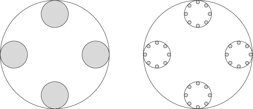
We define a compact fractal set K⊂ℝ2K\subset\mathbb{R}^{2} with κ⁡(K)=π​ℋ1​(K)\kappa(K)=\pi\mathcal{H}^{1}(K) using an iteration procedure. We start with K1=B¯​((0,0),1)K_{1}=\overline{B}((0,0),1) and continue by contracting and copying K1K_{1} as follows. For each integers kk and jj with k≥2k\geq 2 and 1≤j≤2k1\leq j\leq 2^{k} we define, using complex notation, a contractive similitude

fk,j​(x):=2−k​x+(1−2−k)​ej​21−k​π​i.f_{k,j}(x):=2^{-k}x+(1-2^{-k})e^{j2^{1-k}\pi i}.

Using these functions we set

Kk:=⋃(j2,…,jk)f2,j2∘f3,j3∘⋯∘fk,jk(K1),K_{k}:=\bigcup_{(j_{2},\dots,j_{k})}f_{2,j_{2}}\circ f_{3,j_{3}}\circ\cdots\circ f_{k,j_{k}}(K_{1}),

where the union runs over all (k−1)(k-1)-tuples of indices with 1≤ji≤2k1\leq j_{i}\leq 2^{k}, i=2,…,ki=2,\dots,k. We call the balls in this union the construction balls of level kk. Notice that Kk+1⊂KkK_{k+1}\subset K_{k} for every k∈ℕk\in\mathbb{N}. Finally, we set

K:=⋂k=1∞Kk.K:=\bigcap_{k=1}^{\infty}K_{k}.

See Figure 3 for an illustration of the construction.
Refer to caption
Figure 3. Here are approximations of the set KK defined in Example 3.4. On the left is K2K_{2} and on the right one step further refinement, the set K3K_{3}.

We claim that ℋ1​(K)=2\mathcal{H}^{1}(K)=2 and κ⁡(K)=2​π\kappa(K)=2\pi. Taking into account (3.1), it suffices to show that ℋ1​(K)≤2\mathcal{H}^{1}(K)\leq 2 and κ⁡(K)≥2​π\kappa(K)\geq 2\pi.

The inequality ℋ1​(K)≤2\mathcal{H}^{1}(K)\leq 2 follows directly by using the construction balls of level kk as the cover for KK in the definition of the Hausdorff measure and by letting k→∞k\to\infty. Thus, it only remains to show that κ⁡(K)≥2​π\kappa(K)\geq 2\pi.

Let ε>0\varepsilon>0. We show that

(3.5) κ⁡(K)≥(1−ε)​2​π.\kappa(K)\geq(1-\varepsilon)2\pi.

By letting U⊂ℝ2U\subset\mathbb{R}^{2} be an open set containing KK such that each connected component of UU contains only one construction ball of level kk, we may restrict ourselves to estimating κ⁡(K∩B)\kappa(K\cap B) for a construction ball BB of level kk with kk arbitrarily large. Let V⊂UV\subset U be open such that K∩B⊂VK\cap B\subset V. It suffices to show that for each connected component V′V^{\prime} of VV we have ℋ1​(∂V′)≥(1−ε)​π​ℋ1​(V′∩K)\mathcal{H}^{1}(\partial V^{\prime})\geq(1-\varepsilon)\pi\mathcal{H}^{1}(V^{\prime}\cap K). Since ℋ1​(∂V′)≥ℋ1​(∂W)\mathcal{H}^{1}(\partial V^{\prime})\geq\mathcal{H}^{1}(\partial W) for W=conv⁡(V′∩K)W=\mathrm{conv}(V^{\prime}\cap K), it is enough to show that ℋ1​(∂W)≥(1−ε)​π​ℋ1​(V′∩K)\mathcal{H}^{1}(\partial W)\geq(1-\varepsilon)\pi\mathcal{H}^{1}(V^{\prime}\cap K).

Let k0k_{0} be the smallest integer so that WW intersects at least 22 of the level k0k_{0} construction balls. By our assumption on UU we have that k0>kk_{0}>k. The set WW is then contained in a level k0−1k_{0}-1 ball B⁡(x,r)B(x,r). We separate the rest of the proof into two cases:

  • OPENi)\rm i)

    WW intersects exactly 22 level k0k_{0} construction balls.

  • OPENii)\rm ii)

    WW intersects at least 33 level k0k_{0} construction balls.

Let us first consider the case OPENi)\rm i). Since the distance between two level k0k_{0} construction balls is at least

(1−21−k0)​sin⁡(2−k0​π)​r≥(1−22−k0)​2−k0​π​r,(1-2^{1-k_{0}})\sin(2^{-k_{0}}\pi)r\geq(1-2^{2-k_{0}})2^{-k_{0}}\pi r,

we may assume that ℋ1​(V′∩K)≥2−k0​r\mathcal{H}^{1}(V^{\prime}\cap K)\geq 2^{-k_{0}}r. Then, one of the construction balls contains a point of ∂W\partial W that has distance at least 32​(1−22−k0)​2−k0​π​r\frac{3}{2}(1-2^{2-k_{0}})2^{-k_{0}}\pi r to the other construction ball. Thus, we may assume that ℋ1​(V′∩K)≥32​2−k0​r\mathcal{H}^{1}(V^{\prime}\cap K)\geq\frac{3}{2}2^{-k_{0}}r. But then, there exist two points in ∂W\partial W with distance at least 2​(1−22−k0)​2−k0​π​r2(1-2^{2-k_{0}})2^{-k_{0}}\pi r, which then yields

ℋ1​(∂W)≥(1−22−k0)​2​π​r​22−k0≥(1−22−k0)​π​ℋ1​(V′∩K).\mathcal{H}^{1}(\partial W)\geq(1-2^{2-k_{0}})2\pi r2^{2-k_{0}}\geq(1-2^{2-k_{0}})\pi\mathcal{H}^{1}(V^{\prime}\cap K).

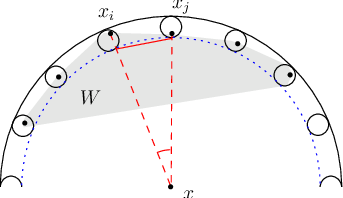
Let us then consider the case OPENii)\rm ii). For each construction level k0k_{0} ball BiB_{i} intersecting WW there exists a point xi∈∂W∩Bix_{i}\in\partial W\cap B_{i}, since none of the balls BiB_{i} is in the convex hull of the other balls. Let us then estimate ℋ1​(∂W)\mathcal{H}^{1}(\partial W) using the angle around the center xx. If xix_{i} and xjx_{j} are contained in adjacent construction balls, the boundary of WW from xix_{i} to xjx_{j} has length at least

(1−21−k0)​sin⁡(αi,j)​r≥(1−22−k0)​αi,j​r,(1-2^{1-k_{0}})\sin(\alpha_{i,j})r\geq(1-2^{2-k_{0}})\alpha_{i,j}r,

where αi,j:=∡⁡(xi,x,xj)\alpha_{i,j}:=\measuredangle(x_{i},x,x_{j}). See Figure 4 for an illustration for the estimate. If xix_{i} and xjx_{j} are not contained in adjacent construction balls, the length of the boundary of WW from xix_{i} to xjx_{j} is at least 21−k0​π2^{1-k_{0}}\pi. All in all, denoting by NN the total number of the construction balls BiB_{i} intersecting WW, we have

ℋ1​(∂W)≥(1−22−k0)​2​π​r​N​2−k0≥(1−22−k0)​π​ℋ1​(V′∩K).\mathcal{H}^{1}(\partial W)\geq(1-2^{2-k_{0}})2\pi rN2^{-k_{0}}\geq(1-2^{2-k_{0}})\pi\mathcal{H}^{1}(V^{\prime}\cap K).
Refer to caption
Figure 4. In the case OPENii)\rm ii), the length of ∂W\partial W is estimated by summing up lengths of projections (red line) of parts connecting points in consecutive balls (here between xix_{i} and xjx_{j}).

4. Proof of the main result

This section is entirely devoted to the proof of Theorem 1.1:

Step 1. Let us denote by {Ei}i=1N\{E_{i}\}_{i=1}^{N} the connected components of ∂Ω\partial\Omega with positive length, where N∈ℕ∪{∞}N\in\mathbb{N}\cup\{\infty\}. We can clearly suppose without loss of generality that N=∞N=\infty. In the case in which Ω\Omega is bounded, we also assume that E1E_{1} is the element containing the boundary of the unbounded connected component of ℝ2∖Ω¯\mathbb{R}^{2}\setminus\overline{\Omega}, which is connected as it is a Jordan loop by Theorem 2.4. Set C≔∂Ω∖⋃i=1∞EiC\coloneqq\partial\Omega\setminus\bigcup_{i=1}^{\infty}E_{i}. Notice that CC can be a Cantor-type set, thus in particular it can have positive ℋ1\mathcal{H}^{1}-measure. Lemma 2.1 grants that

(4.1) ∑i=1∞diam⁡(Ei)≤∑i=1∞ℋ1​(Ei)≤ℋ1​(∂Ω)<+∞.\sum_{i=1}^{\infty}\mathrm{diam}(E_{i})\leq\sum_{i=1}^{\infty}\mathcal{H}^{1}(E_{i})\leq\mathcal{H}^{1}(\partial\Omega)<+\infty.

Consequently, we can relabel the sets {Ei}i≥2\{E_{i}\}_{i\geq 2} so that diam⁡(Ei)≥diam⁡(Ej)\mathrm{diam}(E_{i})\geq\mathrm{diam}(E_{j}) if 2≤i≤j2\leq i\leq j.

Let us fix ε>0\varepsilon>0. For each i∈ℕi\in\mathbb{N}, we select a point zi∈Eiz_{i}\in E_{i}. Observe that

∑i=1∞ℋ∞1​(B⁡(zi,4​diam​(Ei)))≤8​∑i=1∞diam⁡(Ei)≤8​∑i=1∞ℋ1​(Ei)≤8​ℋ1​(∂Ω)<+∞.\sum_{i=1}^{\infty}\mathcal{H}^{1}_{\infty}\big(B(z_{i},4\,\mathrm{diam}(E_{i}))\big)\leq 8\sum_{i=1}^{\infty}\mathrm{diam}(E_{i})\leq 8\sum_{i=1}^{\infty}\mathcal{H}^{1}(E_{i})\leq 8\,\mathcal{H}^{1}(\partial\Omega)<+\infty.

By using the Borel-Cantelli lemma we deduce that ℋ∞1​(⋂k=1∞⋃i=k∞B⁡(zi,4​diam​(Ei)))=0\mathcal{H}^{1}_{\infty}\big(\bigcap_{k=1}^{\infty}\bigcup_{i=k}^{\infty}B(z_{i},4\,\mathrm{diam}(E_{i}))\big)=0. Since ℋ1≪ℋ∞1\mathcal{H}^{1}\ll\mathcal{H}^{1}_{\infty} and the measure ℋ1|∂Ω\mathcal{H}^{1}|_{\partial\Omega} is continuous from above, we see that

limk→∞ℋ1​(∂Ω∩⋃i=k∞B⁡(zi,4​diam​(Ei)))=ℋ1​(∂Ω∩⋂k=1∞⋃i=k∞B⁡(zi,4​diam​(Ei)))=0.\lim_{k\to\infty}\mathcal{H}^{1}\Big(\partial\Omega\cap\bigcup\nolimits_{i=k}^{\infty}B\big(z_{i},4\,\mathrm{diam}(E_{i})\big)\Big)=\mathcal{H}^{1}\Big(\partial\Omega\cap\bigcap\nolimits_{k=1}^{\infty}\bigcup\nolimits_{i=k}^{\infty}B\big(z_{i},4\,\mathrm{diam}(E_{i})\big)\Big)=0.

Therefore, there exists k∈ℕk\in\mathbb{N} such that

(4.2) ℋ1​(∂Ω∩⋃i=k∞B⁡(zi,4​diam​(Ei)))<2​ε5​π,∑i=k∞diam⁡(Ei)<ε10​π.\begin{split}\mathcal{H}^{1}\Big(\partial\Omega\cap\bigcup\nolimits_{i=k}^{\infty}B\big(z_{i},4\,\mathrm{diam}(E_{i})\big)\Big)&<\frac{2\,\varepsilon}{5\,\pi},\\ \sum_{i=k}^{\infty}\mathrm{diam}(E_{i})&<\frac{\varepsilon}{10\,\pi}.\end{split}

Step 2. Choose any continuous curve γ1⊂Ω\gamma_{1}\subset\Omega joining xx to yy. Theorem 3.3 grants that for any i=1,…,k−1i=1,\ldots,k-1 we can choose an open neighbourhood ViV_{i} of EiE_{i} in such a way that

V¯i∩V¯j=∅ for every ​1≤i<j≤k−1,V¯i∩γ1=∅ for every ​i=1,…,k−1,ℋ1​(∂Vi)≤2​ℋ1​(Ei)+2​ε5​(k−1) for every ​i=1,…,k−1.\begin{split}\overline{V}_{i}\cap\overline{V}_{j}=\emptyset&\quad\text{ for every }1\leq i<j\leq k-1,\\ \overline{V}_{i}\cap\gamma_{1}=\emptyset&\quad\text{ for every }i=1,\ldots,k-1,\\ \mathcal{H}^{1}(\partial V_{i})\leq 2\,\mathcal{H}^{1}(E_{i})+\frac{2\,\varepsilon}{5\,(k-1)}&\quad\text{ for every }i=1,\ldots,k-1.\end{split}

We can also assume that the boundary of each set ViV_{i} consists of finitely many pairwise disjoint Jordan loops. Notice that x,yx,y lie in the same connected component of ℝ2∖⋃i=1k−1Vi\mathbb{R}^{2}\setminus\bigcup_{i=1}^{k-1}V_{i}, thanks to the fact that the curve γ1\gamma_{1} does not intersect ⋃i=1k−1Vi\bigcup_{i=1}^{k-1}V_{i}. We distinguish two cases:

  • •

    Ω\Omega is bounded. Let us call Ω′\Omega^{\prime} the (bounded) connected component of ℝ2∖V¯1\mathbb{R}^{2}\setminus\overline{V}_{1} that contains γ1\gamma_{1} (thus also x,yx,y). The boundary of Ω′\Omega^{\prime} is a Jordan loop σ:[0,1]→ℝ2\sigma\colon[0,1]\to\mathbb{R}^{2} with ℓ⁡(σ)≤ℋ1​(∂V1)≤2​ℋ1​(E1)+2​ε5​(k−1)\ell(\sigma)\leq\mathcal{H}^{1}(\partial V_{1})\leq 2\,\mathcal{H}^{1}(E_{1})+\frac{2\,\varepsilon}{5(k-1)} (cf. Theorem 2.4). Possibly reparametrizing σ\sigma, we can suppose to have 0<t1<t2<t3<t4<t5<10<t_{1}<t_{2}<t_{3}<t_{4}<t_{5}<1 such that

    x,y∈(σ0,σt3)⊂Ω′,x∈(σt1,σt5)⊂Ω′,y∈(σt2,σt4)⊂Ω′x,y\in(\sigma_{0},\sigma_{t_{3}})\subset\Omega^{\prime},\quad x\in(\sigma_{t_{1}},\sigma_{t_{5}})\subset\Omega^{\prime},\quad y\in(\sigma_{t_{2}},\sigma_{t_{4}})\subset\Omega^{\prime}

    and the segments [σt1,σt5],[σt2,σt4][\sigma_{t_{1}},\sigma_{t_{5}}],[\sigma_{t_{2}},\sigma_{t_{4}}] are perpendicular to [x,y][x,y]. It readily follows from Lemma 2.1 that |x−σt1|≤ℓ⁡(σ|[0,t1])|x-\sigma_{t_{1}}|\leq\ell(\sigma|_{[0,t_{1}]}), |y−σt2|≤ℓ⁡(σ|[t2,t3])|y-\sigma_{t_{2}}|\leq\ell(\sigma|_{[t_{2},t_{3}]}), |y−σt4|≤ℓ⁡(σ|[t3,t4])|y-\sigma_{t_{4}}|\leq\ell(\sigma|_{[t_{3},t_{4}]}) and |x−σt5|≤ℓ⁡(σ|[t5,0])|x-\sigma_{t_{5}}|\leq\ell(\sigma|_{[t_{5},0]}). Calling ∗* the concatenation of curves, we thus see that

    ℓ⁡([x,σt1]∗σ|[t1,t2]∗[σt2,y])+ℓ⁡([x,σt5]∗σ|[t5,t4]∗[σt4,y])≤ℓ⁡(σ).\ell\big([x,\sigma_{t_{1}}]*\sigma|_{[t_{1},t_{2}]}*[\sigma_{t_{2}},y]\big)+\ell\big([x,\sigma_{t_{5}}]*\sigma|_{[t_{5},t_{4}]}*[\sigma_{t_{4}},y]\big)\leq\ell(\sigma).

    Then we define s:[0,1]→ℝ2s\colon[0,1]\to\mathbb{R}^{2} as the shortest curve between [x,σt1]∗σ|[t1,t2]∗[σt2,y][x,\sigma_{t_{1}}]*\sigma|_{[t_{1},t_{2}]}*[\sigma_{t_{2}},y] and [x,σt5]∗σ|[t5,t4]∗[σt4,y][x,\sigma_{t_{5}}]*\sigma|_{[t_{5},t_{4}]}*[\sigma_{t_{4}},y], so that ℓ⁡(s)≤ℋ1​(E1)+ε5​(k−1)\ell(s)\leq\mathcal{H}^{1}(E_{1})+\frac{\varepsilon}{5(k-1)}. See Figure 5 for the curve ss.

    Refer to caption
    Figure 5. The first approximation ss of the curve is obtained in the bounded case by going near the outer boundary. In the unbounded case, the initial curve is just the line-segment connecting the points.
  • •

    Ω\Omega is unbounded. Then we define s:[0,1]→ℝ2s\colon[0,1]\to\mathbb{R}^{2} as st≔x+t⁡(y−x)s_{t}\coloneqq x+t(y-x) for all t∈[0,1]t\in[0,1].

For the sake of simplicity, let us define the quantity q>0q>0 as

(4.3) q≔{0|x−y| if ​Ω​ is bounded, if ​Ω​ is unbounded.q\coloneqq\left\{\begin{array}[]{ll}0\\ |x-y|\end{array}\quad\begin{array}[]{ll}\text{ if }\Omega\text{ is bounded,}\\ \text{ if }\Omega\text{ is unbounded.}\end{array}\right.
Refer to caption
Figure 6. In the second approximation, the curve is constructed so that it avoids a finite number of the largest boundary components. Next, it is slightly perturbed so that it does not intersect the (remaining) boundary points in a positive ℋ1\mathcal{H}^{1}-measure set.

We proceed in a recursive way: choose that i1∈{1,…,k−1}i_{1}\in\{1,\ldots,k-1\} such that Vi1V_{i_{1}} is the first element of {Vi}i=1k−1\{V_{i}\}_{i=1}^{k-1} that is encountered by the curve ss (note that i1≥2i_{1}\geq 2 if Ω\Omega is bounded). Put a1≔min⁡{t∈(0,1)|st∈∂Vi1}a_{1}\coloneqq\min\big\{t\in(0,1)\,\big|\,s_{t}\in\partial V_{i_{1}}\big\}. The connected component of ∂Vi1\partial V_{i_{1}} containing sa1s_{a_{1}} is the image of a Jordan loop σ1\sigma_{1}. Now let us call b1≔max⁡{t∈(a1,1)|st∈σ1}b_{1}\coloneqq\max\big\{t\in(a_{1},1)\,\big|\,s_{t}\in\sigma_{1}\big\}. Observe that s|(b1,1)∩∂Vi1=∅s|_{(b_{1},1)}\cap\partial V_{i_{1}}=\emptyset. We can write the image of σ1\sigma_{1} as the union of two injective curves α1,α~1\alpha^{1},\tilde{\alpha}^{1} joining sa1s_{a_{1}} to sb1s_{b_{1}}. Given that the length of σ1\sigma_{1} does not exceed ℋ1​(∂Vi1)\mathcal{H}^{1}(\partial V_{i_{1}}), which in turn is smaller than 2​ℋ1​(Ei1)+2​ε5​(k−1)2\,\mathcal{H}^{1}(E_{i_{1}})+\frac{2\,\varepsilon}{5(k-1)}, we can assume without loss of generality that the length of α1\alpha^{1} is smaller than ℋ1​(Ei1)+ε5​(k−1)\mathcal{H}^{1}(E_{i_{1}})+\frac{\varepsilon}{5(k-1)}.

We can now argue in the same way starting from sb1s_{b_{1}}. Take i2∈{1,…,k−1}∖{i1}i_{2}\in\{1,\ldots,k-1\}\setminus\{i_{1}\} such that the first of the sets ViV_{i} that we meet while going from sb1s_{b_{1}} to yy is Vi2V_{i_{2}} (again, i2≠1i_{2}\neq 1 if Ω\Omega is bounded). We denote by a2a_{2} the smallest t∈(b1,1)t\in(b_{1},1) for which st∈∂Vi2s_{t}\in\partial V_{i_{2}}; the connected component of ∂Vi2\partial V_{i_{2}} containing sa2s_{a_{2}} is the image of a Jordan loop σ2\sigma_{2}, and b2b_{2} stands for the biggest t∈(a2,1)t\in(a_{2},1) such that st∈σ2s_{t}\in\sigma_{2}. Then we can find a curve α2\alpha^{2} in σ2\sigma_{2} joining sa2s_{a_{2}} to sb2s_{b_{2}}, which is shorther than ℋ1​(Ei2)+ε5​(k−1)\mathcal{H}^{1}(E_{i_{2}})+\frac{\varepsilon}{5(k-1)}. By repeating this procedure finitely many times (see Figure 6), we obtain a curve γ2\gamma_{2} of the form

γ2≔s|[0,a1]∗α1∗s|[b1,a2]∗α2∗…∗s|[bℓ−1,aℓ]∗αℓ∗s|[bℓ,1]\gamma_{2}\coloneqq s|_{[0,a_{1}]}*\alpha^{1}*s|_{[b_{1},a_{2}]}*\alpha^{2}*\ldots*s|_{[b_{\ell-1},a_{\ell}]}*\alpha^{\ell}*s|_{[b_{\ell},1]}

for some ℓ≤k−1\ell\leq k-1. Notice that γ2\gamma_{2} is contained in ℝ2∖⋃i=1k−1Ei\mathbb{R}^{2}\setminus\bigcup_{i=1}^{k-1}E_{i} and connects xx to yy. By combining the previous estimates, we also deduce that

(4.4) ℓ⁡(γ2)<q+∑i=1k−1ℋ1​(Ei)+ε5.\ell(\gamma_{2})<q+\sum_{i=1}^{k-1}\mathcal{H}^{1}(E_{i})+\frac{\varepsilon}{5}.

Step 3. In light of (4.4), we can choose some points p1,…,p2​h−1∈γ2∖{x,y}p_{1},\ldots,p_{2h-1}\in\gamma_{2}\setminus\{x,y\} having the following property: the curve γ3≔[x,p1]∗[p1,p2]∗…∗[p2​h−2,p2​h−1]∗[p2​h−1,y]\gamma_{3}\coloneqq[x,p_{1}]*[p_{1},p_{2}]*\ldots*[p_{2h-2},p_{2h-1}]*[p_{2h-1},y] is contained in ℝ2∖⋃i=1k−1Ei\mathbb{R}^{2}\setminus\bigcup_{i=1}^{k-1}E_{i} and satisfies

ℓ⁡(γ3)<q+∑i=1k−1ℋ1​(Ei)+ε5.\ell(\gamma_{3})<q+\sum_{i=1}^{k-1}\mathcal{H}^{1}(E_{i})+\frac{\varepsilon}{5}.

Now let us apply Proposition 2.9: we can find some points q1,q3,…,q2​h−1q_{1},q_{3},\ldots,q_{2h-1} (sufficiently near to p1,p3,…,p2​h−1p_{1},p_{3},\ldots,p_{2h-1}, respectively) for which the following conditions are verified:

  • •

    The curve γ4≔[x,q1]∗[q1,p2]∗…∗[p2​h−2,q2​h−1]∗[q2​h−1,y]\gamma_{4}\coloneqq[x,q_{1}]*[q_{1},p_{2}]*\ldots*[p_{2h-2},q_{2h-1}]*[q_{2h-1},y] satisfies

    (4.5) ℓ⁡(γ4)<q+∑i=1k−1ℋ1​(Ei)+ε5,\ell(\gamma_{4})<q+\sum_{i=1}^{k-1}\mathcal{H}^{1}(E_{i})+\frac{\varepsilon}{5},
  • •

    γ4\gamma_{4} is contained in ℝ2∖⋃i=1k−1Ei\mathbb{R}^{2}\setminus\bigcup_{i=1}^{k-1}E_{i},

  • •

    the set γ4∩∂Ω\gamma_{4}\cap\partial\Omega has null ℋ1\mathcal{H}^{1}-measure.

By upper continuity of ℋ1|∂Ω\mathcal{H}^{1}|_{\partial\Omega}, we can find δ>0\delta>0 such that B⁡(γ4,2​δ)⊂ℝ2∖⋃i=1k−1EiB(\gamma_{4},2\,\delta)\subset\mathbb{R}^{2}\setminus\bigcup_{i=1}^{k-1}E_{i} and

(4.6) ℋ1​(∂Ω∩B⁡(γ4,2​δ))<2​ε5​π.\mathcal{H}^{1}\big(\partial\Omega\cap B(\gamma_{4},2\,\delta)\big)<\frac{2\,\varepsilon}{5\,\pi}.

Theorem 3.3 provides an open neighbourhood U′⊂B⁡(γ4,δ)∖⋃i=1k−1EiU^{\prime}\subset B(\gamma_{4},\delta)\setminus\bigcup_{i=1}^{k-1}E_{i} of γ4\gamma_{4} such that

(4.7) ℋ1​(∂U′)≤2​ℓ​(γ4)+2​ε5≤2​q+2​∑i=1k−1ℋ1​(Ei)+4​ε5,\mathcal{H}^{1}(\partial U^{\prime})\leq 2\,\ell(\gamma_{4})+\frac{2\,\varepsilon}{5}\leq 2\,q+2\sum_{i=1}^{k-1}\mathcal{H}^{1}(E_{i})+\frac{4\,\varepsilon}{5},

where the second inequality stems from (4.5). Moreover, let us fix any index m≥km\geq k for which diam⁡(Em)<dist⁡(γ4,∂U′)\mathrm{diam}(E_{m})<\mathrm{dist}(\gamma_{4},\partial U^{\prime}). Since i↦diam⁡(Ei)i\mapsto\mathrm{diam}(E_{i}) is non-increasing for i≥ki\geq k, one has

(4.8) diam⁡(Ei)<dist⁡(γ4,∂U′) for every ​i≥m.\mathrm{diam}(E_{i})<\mathrm{dist}(\gamma_{4},\partial U^{\prime})\quad\text{ for every }i\geq m.

Let us define

U≔U′∪⋃i=kmB⁡(zi,2​diam​(Ei)).U\coloneqq U^{\prime}\cup\bigcup_{i=k}^{m}B\big(z_{i},2\,\mathrm{diam}(E_{i})\big).

See Figure 7 for an illustration of the set UU.

Refer to caption
Figure 7. The final curve is found inside a set UU that is obtained as the union of a neighbourhood of the curve γ4\gamma_{4} and suitable collection of balls. The neighbourhood of γ4\gamma_{4} allows us to avoid the largest pieces of the boundary, which the curve γ4\gamma_{4} avoided. By taking balls around the remaining boundary parts that have so large diameter that they could block inside the previous neighbourhood, we are guaranteed to be able to connect xx to yy inside UU.

Given that U¯⊂B⁡(γ4,2​δ)∪⋃i=kmB⁡(zi,4​diam​(Ei))\overline{U}\subset B(\gamma_{4},2\,\delta)\cup\bigcup_{i=k}^{m}B\big(z_{i},4\,\mathrm{diam}(E_{i})\big), we deduce from the first line of (4.2) and from (4.6) that

(4.9) ℋ1​(∂Ω∩U¯)<4​ε5​π.\mathcal{H}^{1}(\partial\Omega\cap\overline{U})<\frac{4\,\varepsilon}{5\,\pi}.

Step 4. We claim that

(4.10) x,y​ belong to the same connected component of ​U∖∂Ω.x,y\text{ belong to the same connected component of }U\setminus\partial\Omega.

We argue by contradiction: suppose that yy does not belong to the connected component AA of U∖∂ΩU\setminus\partial\Omega containing xx. Call BB the connected component of ℝ2∖A\mathbb{R}^{2}\setminus A that contains yy (notice that yy lies in the interior of BB). Call FF the connected component of ∂A\partial A that is included in BB. Hence, Lemma 2.2 yields F=∂BF=\partial B. Given that γ4\gamma_{4} joins x∉Bx\notin B to y∈By\in B, we deduce that γ4∩∂B≠∅\gamma_{4}\cap\partial B\neq\emptyset. Choose any z∈γ4∩∂Bz\in\gamma_{4}\cap\partial B. Observe that ∂B⊂∂A⊂∂U∪∂Ω\partial B\subset\partial A\subset\partial U\cup\partial\Omega, thus the fact that γ4⊂U\gamma_{4}\subset U gives z∈∂Ωz\in\partial\Omega. Call EE the connected component of ∂Ω\partial\Omega containing zz. Given that γ4⊂ℝ2∖⋃i=1k−1Ei\gamma_{4}\subset\mathbb{R}^{2}\setminus\bigcup_{i=1}^{k-1}E_{i}, we have that either E=EiE=E_{i} for some i≥ki\geq k or E⊂CE\subset C. To prove that E∩∂U=∅E\cap\partial U=\emptyset we distinguish the following three cases:

  • OPENi)\rm i)

    E=EiE=E_{i} for some i=k,…,mi=k,\ldots,m. Then it holds E⊂B⁡(zi,2​diam​(Ei))⊂UE\subset B\big(z_{i},2\,\mathrm{diam}(E_{i})\big)\subset U, whence accordingly E∩∂U=∅E\cap\partial U=\emptyset.

  • OPENii)\rm ii)

    E=EiE=E_{i} for some i>mi>m. Since diam⁡(E)<dist⁡(γ4,∂U′)\mathrm{diam}(E)<\mathrm{dist}(\gamma_{4},\partial U^{\prime}) by (4.8) and γ4∩E≠∅\gamma_{4}\cap E\neq\emptyset, we see that E⊂U′⊂UE\subset U^{\prime}\subset U and thus E∩∂U=∅E\cap\partial U=\emptyset.

  • OPENiii)\rm iii)

    E⊂CE\subset C. Then EE is a non-empty connected set with null diameter, namely a singleton, so that clearly E∩∂U=∅E\cap\partial U=\emptyset.

Therefore, EE is also a connected component of ∂U∪∂Ω\partial U\cup\partial\Omega and accordingly ∂B⊂E\partial B\subset E. The set ℝ2∖∂B\mathbb{R}^{2}\setminus\partial B cannot be connected, otherwise we would have B̊=ℝ2∖∂B\mathring{B}=\mathbb{R}^{2}\setminus\partial B and thus B=ℝ2B=\mathbb{R}^{2}. Therefore, ℝ2∖∂B\mathbb{R}^{2}\setminus\partial B has at least two connected components: one coincides with B̊\mathring{B} (thus contains yy), while another one contains the point xx. Then any curve joining xx to yy must intersect ∂B⊂∂Ω\partial B\subset\partial\Omega, which is in contradiction with the assumption that Ω\Omega is connected. Consequently, the claim (4.10) is proven.
Step 5. Thanks to (4.10), we can find a continuous curve γ5⊂U∖∂Ω\gamma_{5}\subset U\setminus\partial\Omega joining xx to yy. The Painlevé estimate (for general compact sets), namely Proposition 3.2, provides us with an open neighbourhood VV of ∂Ω∩U¯\partial\Omega\cap\overline{U} such that V¯∩γ5=∅\overline{V}\cap\gamma_{5}=\emptyset and

(4.11) ℋ1​(∂V)≤π​ℋ1​(∂Ω∩U¯)<4​ε5,\mathcal{H}^{1}(\partial V)\leq\pi\,\mathcal{H}^{1}(\partial\Omega\cap\overline{U})<\frac{4\,\varepsilon}{5},

where the second inequality is a consequence of (4.9). Let us denote by W′W^{\prime} the connected component of U∖V¯U\setminus\overline{V} containing γ5\gamma_{5}. Note that ∂W′⊂∂U′∪∂V∪⋃i=km∂B⁡(zi,2​diam​(Ei))\partial W^{\prime}\subset\partial U^{\prime}\cup\partial V\cup\bigcup_{i=k}^{m}\partial B\big(z_{i},2\,\mathrm{diam}(E_{i})\big). Therefore, by combining the estimates in (4.7), in (4.11) and in the second line of (4.2), we conclude that ℋ1​(∂W′)<2​(q+∑i=1k−1ℋ1​(Ei)+ε)\mathcal{H}^{1}(\partial W^{\prime})<2\big(q+\sum_{i=1}^{k-1}\mathcal{H}^{1}(E_{i})+\varepsilon\big). Since γ5⊂W′⊂W′¯⊂ℝ2∖∂Ω\gamma_{5}\subset W^{\prime}\subset\overline{W^{\prime}}\subset\mathbb{R}^{2}\setminus\partial\Omega, we can apply Proposition 2.14 to obtain a bounded domain W⊂ℝ2W\subset\mathbb{R}^{2} with γ5⊂W⊂Ω\gamma_{5}\subset W\subset\Omega, whose boundary is the disjoint union of finitely many smooth Jordan loops and such that

(4.12) ℋ1​(∂W)<2​(q+∑i=1k−1ℋ1​(Ei)+ε).\mathcal{H}^{1}(\partial W)<2\Big(q+\sum\nolimits_{i=1}^{k-1}\mathcal{H}^{1}(E_{i})+\varepsilon\Big).

We call λ\lambda the boundary of the unbounded connected component of ℝ2∖W¯\mathbb{R}^{2}\setminus\overline{W}, while by {λj}j∈J\{\lambda_{j}\}_{j\in J} (for some finite family of indices JJ) we denote the boundaries of the bounded connected components of ℝ2∖W¯\mathbb{R}^{2}\setminus\overline{W}. Let us also define Λ≔⋃j∈Jλj\Lambda\coloneqq\bigcup_{j\in J}\lambda_{j}.
Step 6. Call LxL_{x} and LyL_{y} the lines orthogonal to [x,y][x,y] that pass through xx and yy, respectively. Take those points u1,u2,u3,u4∈λu_{1},u_{2},u_{3},u_{4}\in\lambda such that x∈[u1,u3]⊂Lxx\in[u_{1},u_{3}]\subset L_{x}, y∈[u2,u4]⊂Lyy\in[u_{2},u_{4}]\subset L_{y}, and (u1,u3)∩λ,(u2,u4)∩λ=∅(u_{1},u_{3})\cap\lambda,(u_{2},u_{4})\cap\lambda=\emptyset. We can suppose that u1,u2u_{1},u_{2} lie in the same connected component of ℝ2∖ℝ⁡(y−x)\mathbb{R}^{2}\setminus\mathbb{R}(y-x) (thus u3,u4u_{3},u_{4} are contained in the other one). By u1​u2wideparen\wideparen{u_{1}u_{2}} we mean the arc in λ\lambda joining u1u_{1} to u2u_{2} that does not contain any other point uiu_{i}, similarly for u3​u4wideparen\wideparen{u_{3}u_{4}} and so on. The set ℝ⁡(y−x)∖[x,y]\mathbb{R}(y-x)\setminus[x,y] is the union of two half-lines; both of them intersect the curve λ\lambda, say at some points u5∈u1​u3wideparenu_{5}\in\wideparen{u_{1}u_{3}} and u6∈u2​u4wideparenu_{6}\in\wideparen{u_{2}u_{4}}. By Lemma 2.1 we see that

(4.13) |x−u1|≤ℋ1​(u1​u5wideparen),|y−u2|≤ℋ1(u2​u6wideparen),|x−u3|≤ℋ1​(u3​u5wideparen),|y−u4|≤ℋ1​(u4​u6wideparen).\begin{split}|x-u_{1}|\leq\mathcal{H}^{1}(\wideparen{u_{1}u_{5}}),\quad&|y-u_{2}|\leq\mathcal{H}^{1}(\wideparen{u_{2}u_{6}}),\quad\\ |x-u_{3}|\leq\mathcal{H}^{1}(\wideparen{u_{3}u_{5}}),\quad&|y-u_{4}|\leq\mathcal{H}^{1}(\wideparen{u_{4}u_{6}}).\end{split}

Let us define the curves γ6,γ7\gamma_{6},\gamma_{7} as

γ6≔[x,u1]∗u1​u2wideparen∗[u2,y],γ7≔[x,u3]∗u3​u4wideparen∗[u4,y].\gamma_{6}\coloneqq[x,u_{1}]*\wideparen{u_{1}u_{2}}*[u_{2},y],\qquad\gamma_{7}\coloneqq[x,u_{3}]*\wideparen{u_{3}u_{4}}*[u_{4},y].

Therefore, (4.13) ensures that ℓ⁡(γ6)+ℓ⁡(γ7)≤ℓ⁡(λ)\ell(\gamma_{6})+\ell(\gamma_{7})\leq\ell(\lambda), whence (possibly relabeling γ6\gamma_{6} and γ7\gamma_{7}) it holds that ℓ⁡(γ6)≤ℓ⁡(λ)/2\ell(\gamma_{6})\leq\ell(\lambda)/2. Finally, it can be readily checked that it is possible to find a curve γ⊂γ6∪Λ\gamma\subset\gamma_{6}\cup\Lambda joining xx to yy such that γ∩∂Ω=∅\gamma\cap\partial\Omega=\emptyset (thus γ⊂Ω\gamma\subset\Omega) and ℋ1​(γ∩Λ)≤ℋ1​(Λ)/2\mathcal{H}^{1}(\gamma\cap\Lambda)\leq\mathcal{H}^{1}(\Lambda)/2. Consequently, we deduce that ℓ⁡(γ)≤ℓ⁡(γ6)+ℋ1​(γ∩Λ)≤(ℓ⁡(λ)+ℋ1​(Λ))/2=ℋ1​(∂W)/2\ell(\gamma)\leq\ell(\gamma_{6})+\mathcal{H}^{1}(\gamma\cap\Lambda)\leq\big(\ell(\lambda)+\mathcal{H}^{1}(\Lambda)\big)/2=\mathcal{H}^{1}(\partial W)/2. By recalling the inequality (4.12), we conclude that ℓ⁡(γ)≤q+∑i=1k−1ℋ1​(Ei)+ε\ell(\gamma)\leq q+\sum_{i=1}^{k-1}\mathcal{H}^{1}(E_{i})+\varepsilon. In view of (4.3), this explicitly means that

ℓ⁡(γ)≤{∑i=1k−1ℋ1​(Ei)+ε|x−y|+∑i=1k−1ℋ1​(Ei)+ε if ​Ω​ is bounded, if ​Ω​ is unbounded.\ell(\gamma)\leq\left\{\begin{array}[]{ll}\sum_{i=1}^{k-1}\mathcal{H}^{1}(E_{i})+\varepsilon\\ |x-y|+\sum_{i=1}^{k-1}\mathcal{H}^{1}(E_{i})+\varepsilon\end{array}\quad\begin{array}[]{ll}\text{ if }\Omega\text{ is bounded,}\\ \text{ if }\Omega\text{ is unbounded.}\end{array}\right.

By arbitrariness of ε>0\varepsilon>0, this completes the proof of Theorem 1.1.

References

  • [1] Giovanni Alberti and Martino Ottolini, On the structure of continua with finite length and Gołąb’s semicontinuity theorem, Nonlinear Analysis 153 (2017), 35–55.
  • [2] L. Ambrosio, N. Fusco, and D. Pallara, Functions of bounded variation and free discontinuity problems, Oxford Science Publications, Clarendon Press, 2000.
  • [3] B. Bollobás, Modern graph theory, Graduate texts in mathematics, Springer, 1998.
  • [4] James J. Dudziak, Vitushkin’s conjecture for removable sets, Universitext, Springer, New York, 2010. MR 2676222
  • [5] Hrant Hakobyan and David A. Herron, Euclidean quasiconvexity., Annales Academiae Scientiarum Fennicae. Mathematica 33 (2008), no. 1, 205–230 (eng).
  • [6] Sergei Kalmykov, Leonid V. Kovalev, and Tapio Rajala, Removable sets for intrinsic metric and for holomorphic functions, J. Anal. Math., to appear, arXiv:1707.07363 (2017).