A Distributionally Robust Boosting Algorithm

Distributional robustness in decision making under uncertainty is an important topic with a long and successful history in the Operations Research literature [2, 22, 3, 13]. In recent years, this topic has been further fueled by distributionally robust optimization (DRO) formulations applied to machine learning and statistical analysis. These formulations have been shown to produce powerful insights in terms of interpretability, parameter tuning, implementation of computational procedures and the ability to enforce performance guarantees.

For instance, the work of [28] studied connections between the statistical theory of Empirical Likelihood and distributionally robust decision making formulations. These connections have been helpful in order to obtain statistical guarantees in a large and important class of data-driven DRO problems.

The work of [15] showed how DRO can be used to establish a connection to regularized logistic regression, therefore explaining the role of regularization in the context of improving out-of-sample performance and data-driven decision-making.

The works of [6, 4] further show that square-root Lasso, support vector machines, and other estimators such as group-Lasso can be recovered exactly from DRO formulations. In turn, in [6], it is shown that exploiting the DRO formulation leads to an optimality criterion for choosing the associated regularization parameter in regularized estimators which is both by robustness and statistical principles. Importantly, such criterion is closely aligned with a well-developed theory of high-dimensional statistics, but the criterion can be used even in the context of non-linear decision making problems.

The work of [12] shows that variance regularization estimation can be cast in terms of a DRO formulation which renders the implementation of such estimator both practical and amenable to rigorous statistical and computational guarantees.

The list of recent papers that exploit DRO for the design of statistical estimators, revisiting classical ideas to improve parameter tuning, interpretation or implementation task is rapidly growing (see in [6, 4, 5, 8, 7, 14, 37, 21, 12]).

This paper contributes to these rapidly-expanding research activities by showing that DRO can naturally be used in the context of boosting statistical procedures. In particular, we are able to show that Adaptive Boosting (AdaBoost) can be viewed as a particular example of DRO-Boosting with a suitable loss function and size of uncertainty, see Corollary 2.

These connections, as indicated earlier, are useful to enhance interpretability. Further, as we explain, DRO provides a systematic and disciplined approach for designing boosting methods. Also, the DRO formulation can be naturally used to fit tuning parameters (such as the strength used to weight one model versus another in the face of statistical evidence) in a statistically principled way.

Finally, we provide easy-to-implement algorithms which can be used to apply our boosting methods, which we refer to as DRO-Boosting procedures.

As an application of our proposed family of procedures, we consider a classification problem in the context of a credit card default payment prediction problem. We find that our approach compares favorably to alternative boosting methods which are widely used in practice.

The rest of this paper is organized as follows. In Section 2 we provide a general discussion about boosting algorithms. This section also introduces various notations which are useful to formulate our problem. Section 3 contains a precise description of the algorithm and the results validating the correctness of the algorithms. We discuss in this section also a connection to AdaBoost. Section 4 contains statistical analysis for the optimal selection of tuning parameters (such as the weight assigned to different models in the presence of available evidence). In Section 5, we show the result of our algorithms in the context of an application to credit card default payments. In Section 6, we summarize the proofs of technical results.

We first start by describing a wide class of boosting algorithms. For concreteness, the reader may focus on a standard supervised classification framework. The ultimate goal is to predict the label $Y$ associated with a predictive variable $X$. We then discuss our DRO problem formulation.

In this section, we propose an algorithm based on functional gradient descent to solve the DRO-Boosting (2). As we shall see, similar to the AdaBoost algorithm as in [20], fitting the DRO-Boosting algorithm exhibits a procedure that alternates between reweighting the worst case probability distribution and updating the predicting function $F(\cdot)$. Therefore, the connection between DRO-Boosting and AdaBoost will be naturally established. Moreover, since choosing different types of distributional uncertainty sets, $\mathcal{U}_{\delta}(P_{N})$, potentially based on different notions of discrepancies between $P_{N}$ and alternative distributions results in different reweighting regimes, it can be speculated that our proposed DRO-Boosting framework is more flexible than AdaBoost.

For ease of notation and introduction of our functional gradient descent method, in the rest of this paper, we define two functionals. For any index $i=\overline{1,N}$, the empirical loss functional $\mathcal{L}_{i}:\mathrm{Lin}(\mathcal{F})\rightarrow\mathbb{R}$ is defined as $\mathcal{L}_{i}(F)=L\left(F\left(X_{i}\right),Y_{i}\right).$ The robust loss functional $\mathcal{L}_{rob}:\mathrm{Lin}(\mathcal{F})\rightarrow\mathbb{R}$ is defined as $\mathcal{L}_{rob}(F)=\max_{P\in\mathcal{U}(P_{N})}\mathbb{E}_{P}\left[L\left(F\left(X\right),Y\right)\right].$

Due to the fact that any finitely supported distribution, $P$, is characterized by its associated weights, $\bm{\omega}_{P}$, we can introduce the weight uncertainty set $\Omega_{\delta}(P_{N})$ defined as

as an isomorphic counterpart of the distributional uncertainty set $\mathcal{U}_{\delta}(P_{N})$.

Thus, using the right hand side weight vector $\bm{\omega}_{P}$ and the weight uncertainty set $\Omega_{\delta}(P_{N})$, the functional $\mathcal{L}_{rob}$ can be rewritten as

We denote by $\Omega_{rob}^{\star}(F)$ the set of all maximizers to the above optimization problem, i.e.

Using these definitions, the DRO-Boosting formulation (2) admits an alternative expression, namely,

consequently it suffices to find a best predicting function $F$ that minimizes $\mathcal{L}_{rob}(F)$. In order to guarantee that the optimization problem (4) has optimal solution, we impose the following assumption.

Next, to simplify the exposition, we impose an assumption which guarantees that the data is rich enough relative to the class $\mathrm{Lin}(\mathcal{F})$. We will discuss how can one proceed if this assumption is violated.

Observation 1: There are natural situations in which the Separation Assumption may fail to hold. For example, if $f_{r}\in\mathcal{F}$ is a regression tree, namely, $f_{t}\left(x\right)=\sum_{j=1}^{m_{t}}I_{A_{j}}\left(x\right),$ where the $A_{j}$’s are disjoint sets forming a partition on the domain of $x$, then when considering $\mathrm{Lin}(\mathcal{F})$ we may violate the Separation Assumption may not hold. Nevertheless, we can define an equivalence relationship “$\sim$” defined via $F\sim G$ if and only if $F(X)=G(X)$ for all $X\in\mathcal{D}_{N}$, and then work with equivalence classes instead. Moreover, since the dimension of the quotient space is at most $N$, we may assume that $\mathrm{Lin}(\mathcal{F})$ is a finite dimensional space without loss of generality. To ease the exposition, we will state the assumption $\mathrm{Lin}(\mathcal{F})$ is finite dimensional next.

If the dimension of $\mathrm{Lin}(\mathcal{F})$ is infinite, then $T$ will grow with $N$ and this will have consequences for the rate of convergence of the algorithm and the statistical analysis of the uncertainty set selection. But this is not important to implement and run the algorithms that we will present below.

We now are ready to summarize some properties of $\mathcal{L}_{rob}$ in Lemma 1 and thereafter develop a subgradient descent algorithm to find the optimal robust decision rule by solving (2).

The predicting function controls the value of $\mathcal{L}_{rob}(F)$ solely via $F(X_{i})$. Thus, to derive the functional gradient descent algorithm, one needs to construct a metric on $\mathcal{F}$ where the structure is determined only by $F(X_{i})$ as well. To this end, we consider the inner product $\langle\cdot,\cdot\rangle_{\mathcal{D}_{N}}$, where

Due to the Assumption 2, $\langle\cdot,\cdot\rangle_{\mathcal{D}_{N}}$ is a well defined inner product on space $\mathrm{Lin}(\mathcal{F})$, and we denote by $\|\cdot\|_{\mathcal{D}_{N}}$ the induced norm of $\langle\cdot,\cdot\rangle_{\mathcal{D}_{N}}$ on $\mathrm{Lin}(\mathcal{F})$. As the dimension of space $\mathrm{Lin}(\mathcal{F})$ can be assumed to be finite due to Observation 1, the space $\mathrm{Lin}(\mathcal{F})$ endowed with inner product $\langle\cdot,\cdot\rangle_{\mathcal{D}_{N}}$ is a Hilbert space. Note that the topology induced by $\langle\cdot,\cdot\rangle_{\mathcal{D}_{N}}$ is isomorphic to the Euclidean topology in $\mathbb{R}^{N}$.

In order to formalize the functional subgradient algorithm, we first introduce the definition of functional subgradient and functional sub-differential.

Using Proposition 1 and Corollary 1, we can make sense of the functional sub-differential $\partial\mathcal{L}_{rob}(F)$ or even the functional gradient $\nabla\mathcal{L}_{rob}(F)$. However, in order to ensure the trajectory of functional gradient descent lies in the space $\mathrm{Lin}(\mathcal{F})$, one wants to find a weak linear in $\mathcal{F}$ to approximate the functional gradient $\mathcal{G}$. This simply means finding a best approximation in $\Pi_{\mathcal{F}}(\mathcal{G})$ such that $\Pi_{\mathcal{F}}(\mathcal{G})=\arg\min_{F\in\mathcal{F}}\|F-\mathcal{G}\|_{\mathcal{D}_{N}}.$

Using these observation, the functional subgradient descent algorithm for solving the DRO-Boosting problem (2) is given in Algorithm 1.

Note that in Algorithm 1, we have to compute a worst case probability weight $\bm{\omega}^{\star}\in\Omega_{rob}^{\star}(F)$ for some functional $F$. If $\mathcal{L}_{1}(F)=\cdots=\mathcal{L}_{N}(F)$, we can simply pick $\bm{\omega}^{\star}=\bm{\omega}_{P_{N}}=(1/N,\ldots,1/N)$. Otherwise, the worst case probability can be computed using the Lemma 2.

Corollary 2 shows that Algorithm 1 exactly recovers the AdaBoost algorithm proposed in [19]. The proof of Corollary 2 is elementary.

Now, note that Algorithm 1 requires supplying the parameter $\delta$. This parameter is typically chosen using cross-validation. However, when $\ \mathrm{Lin}(\mathcal{F})=\mathrm{Lin}\{f_{1},...,f_{T}\}$, with $T$ fixed, we can use the work of [12, 28], which establishes a connection to Empirical Likelihood to obtain $\delta$. This will be discussed in Section 4.

We now explain how to choose $\delta$ using statistical principles and avoiding cross-validation. The strategy is to invoke the theory of Empirical Likelihood, following the approach in [28, 5], as we shall explain. We assume that the data $\mathcal{D}_{N}=\{\left(X_{i},Y_{i}\right)_{i=1}^{N}\}$ is i.i.d. from an underlying distribution $P_{\ast}$, which is unknown. We use $P_{\ast}^{\infty}$ to denote the product measure $P_{\ast}\times P_{\ast}\times...$ governing the distribution of the whole sequence $\{\left(X_{n},Y_{n}\right):n\geq 1\}$. Moreover, in this section we will assume, in Assumption 3, that $\mathrm{Lin}(\mathcal{F})=\mathrm{Lin}\{f_{1},...,f_{T}\}$ where $T$ is fixed and independent of $N$.

For each probability measure $P$, there is an associated optimal predicting function $F$ as the minimizer to the risk minimization problem $F^{P}=\arg\min_{F\in\mathrm{Lin}(\mathcal{F})}\mathbb{E}_{P}\left[L\left(F\left(X\right),Y\right)\right].$ We assume the convexity and smoothness for the loss function as discussed previously in Section 3. Following the criterion discussed in [5], we define $\Lambda_{\delta}\left(P_{N}\right)=\{F^{P}:P\in\mathcal{U}_{\delta}(P_{N})\}.$ The set $\Lambda_{\delta}\left(P_{N}\right)$ can be interpreted as a confidence region for the functional parameter $F^{P_{\ast}}$ and we are interested in minimizing the size of the confidence region, $\delta$, while guaranteeing a desired level of coverage for the confidence region $\Lambda_{\delta}\left(P_{N}\right)$. In other words, we want to choose $\delta$ as the solution to the problem

where $1-\alpha$ is a desired confidence level, say 95%, which implies choosing $\alpha=.05$. This problem is challenging to solve, but we will provide an asymptotic approximation to it as $N\rightarrow\infty$.

We make the following assumptions to proceed the discussion.

By the definition of the functional gradient in Definition 1, we know $\nabla_{F}L\left(F^{P}\left(X\right),Y\right)\in\mathbb{R}^{T}$.

The derivation of the asymptotic results relies on central limitation theorem, and we assume the existence of the second moment for the functional gradient.

In order to compute $\delta$ according to (7) we will provide a more convenient representation for the set $\{F^{P_{\ast}}\in\Lambda_{\delta}\left(P_{N}\right)\}$. For any $F$, we can define a set of probability measures $M\left(F\right)$ for which $F$ is an optimal boosting learner, that is, $P\in M\left(F\right)$ if $\mathbb{E}_{P}\left[\nabla_{F}L\left(F\left(X\right),Y\right)\right]=0$. Consequently,

Define the smallest Kullback-Leibler discrepancy between $P_{N}$ and any element of $M\left(F\right)$ via

It is immediate to see that $F^{P_{\ast}}\in\Lambda_{\delta}\left(P_{N}\right)$ if and only if there exists an element in $P\in M\left(F^{P_{\ast}}\right)$ such that $D(P\|P_{N})\leq\delta$. Consequently, we have

The asymptotic analysis of the object $R_{N}\left(F^{P_{\ast}}\right)$, known as the Empirical Profile Likelihood (EPL) has been studied extensively. From (9) we have that the solution to (7) is precisely the $1-\alpha$ quantile of $R_{N}\left(F^{P_{\ast}}\right)$. Therefore, to approximate $\delta$, it suffices to estimate the asymptotic distribution of $R_{N}\left(F^{P_{\ast}}\right)$.

We apply the techniques in [28] to derive the asymptotic distribution of $R_{N}\left(F\right)$ as $n\rightarrow\infty$, and pick the $1-\alpha$ quantile of the asymptotic distribution as our uncertainty size.

Figure 1 gives an illustration of the equivalence in (9). The emphasized line corresponds to the Kullback-Leibler divergence between the empirical distribution and the manifold $M\left(F^{P_{\ast}}\right)$.

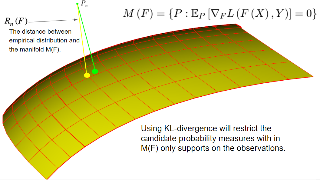
The asymptotic results for (8) is similar as introduced in the literature for the empirical likelihood theorem as in [32, 34, 33]. There show that the asymptotic distribution is chi-square and the degree of freedom depends on the estimating equation. We state the results in Theorem 1 below.

We can notice the rate of convergence is free of the data dimension and the dimension of the dimension of the functional space. Theorem 1 is a generalization of the empirical likelihood theorem for general estimating equation introduced in [34].

In this section, we apply our DRO-Boosting algorithm to predict default in credit card payment. We take the credit-card default payment data of Taiwan from UCI machine learning database [29]. The data has 23 predictors and the response is binary stands for non-default and default. There are 30000 observations in the data set with 6636 defaults and 23364 non-defaults.

We take the binary classification tree as the weak learner as the basis function, and we consider exponential loss function for model fitting. We compare our model with the AdaBoost algorithm, which is the state-of-art boosting algorithm for practical consideration.

Every time, we randomly split the data into a training set, with 3000 observations, and a testing set, with the rest 27000 data points. We train the model on the training set as we illustrated in Algorithm 1. We consider the basis function as 5-layer classification tree, and we assume the dimension (or effective degree of freedom) of the functional space is roughly 30. To pick the uncertainty set, we apply the method introduced in Section 4, where we pick the level of uncertainty to be $90\%$. We consider a more complex basis model, a 5-layer classification tree, as the weak learner, which is mainly due to we try to explore a case where the AdaBoost model is more likely to overfit the data.

We report the accuracy, true positive rate, false negative rate, and the exponential loss in Table 1, where we can observe superior performance for the DRO-Boosting model on the testing set.

We can observe from our numerical experiment that the DRO formalization helps improve the performance on the testing set. The worst-case expected loss function tires to mimic the testing error and avoid overemphasis on the training set. Thus we observe higher training error using DRO, while the advantage is reflected in the testing error.

References

- Bayraksan and Love, [2015] Bayraksan, G. and Love, D. K. (2015). Data-driven stochastic programming using phi-divergences. In The Operations Research Revolution, pages 1–19. INFORMS.
- Ben-Tal and Nemirovski, [2000] Ben-Tal, A. and Nemirovski, A. (2000). Robust solutions of linear programming problems contaminated with uncertain data. Mathematical programming, 88(3):411–424.
- Bertsimas and Sim, [2004] Bertsimas, D. and Sim, M. (2004). The price of robustness. Operations research, 52(1):35–53.
- [4] Blanchet, J. and Kang, Y. (2017a). Distributionally robust groupwise regularization estimator. Manuscript.
- [5] Blanchet, J. and Kang, Y. (2017b). Distributionally robust semi-supervised learning. arXiv preprint arXiv:1702.08848.
- Blanchet et al., [2016] Blanchet, J., Kang, Y., and Murthy, K. (2016). Robust wasserstein profile inference and applications to machine learning. arXiv preprint arXiv:1610.05627.
- [7] Blanchet, J., Kang, Y., Zhang, F., He, F., and Hu, Z. (2017a). Doubly robust data-driven distributionally robust optimization. arXiv preprint arXiv:1705.07168.
- [8] Blanchet, J., Kang, Y., Zhang, F., and Murthy, K. (2017b). Data-driven optimal transport cost selection for distributionally robust optimizatio. arXiv preprint arXiv:1705.07152.
- Blanchet and Murthy, [2016] Blanchet, J. and Murthy, K. (2016). Quantifying distributional model risk via optimal transport.
- Delage and Ye, [2010] Delage, E. and Ye, Y. (2010). Distributionally robust optimization under moment uncertainty with application to data-driven problems. Operations research, 58(3):595–612.
- Drucker, [1997] Drucker, H. (1997). Improving regressors using boosting techniques. In Proceedings of the Fourteenth International Conference on Machine Learning, pages 107–115. Morgan Kaufmann Publishers Inc.
- Duchi et al., [2016] Duchi, J., Glynn, P., and Namkoong, H. (2016). Statistics of robust optimization: A generalized empirical likelihood approach. arXiv preprint arXiv:1610.03425.
- Erdoğan and Iyengar, [2006] Erdoğan, E. and Iyengar, G. (2006). Ambiguous chance constrained problems and robust optimization. Mathematical Programming, 107(1-2):37–61.
- Esfahani and Kuhn, [2015] Esfahani, P. M. and Kuhn, D. (2015). Data-driven distributionally robust optimization using the wasserstein metric: Performance guarantees and tractable reformulations. arXiv preprint arXiv:1505.05116.
- Esfahani and Kuhn, [2018] Esfahani, P. M. and Kuhn, D. (2018). Data-driven distributionally robust optimization using the wasserstein metric: Performance guarantees and tractable reformulations. Mathematical Programming, 171(1-2):115–166.
- Fathony et al., [2018] Fathony, R., Rezaei, A., Bashiri, M. A., Zhang, X., and Ziebart, B. (2018). Distributionally robust graphical models. In Advances in Neural Information Processing Systems, pages 8354–8365.
- Freund, [1995] Freund, Y. (1995). Boosting a weak learning algorithm by majority. Information and computation, 121(2):256–285.
- Freund, [2009] Freund, Y. (2009). A more robust boosting algorithm. arXiv preprint arXiv:0905.2138.
- Freund and Schapire, [1997] Freund, Y. and Schapire, R. E. (1997). A decision-theoretic generalization of on-line learning and an application to boosting. Journal of computer and system sciences, 55(1):119–139.
- Friedman, [2001] Friedman, J. H. (2001). Greedy function approximation: a gradient boosting machine. Annals of statistics, pages 1189–1232.
- Gao and Kleywegt, [2016] Gao, R. and Kleywegt, A. J. (2016). Distributionally robust stochastic optimization with wasserstein distance. arXiv preprint arXiv:1604.02199.
- Ghaoui et al., [2003] Ghaoui, L. E., Oks, M., and Oustry, F. (2003). Worst-case value-at-risk and robust portfolio optimization: A conic programming approach. Operations research, 51(4):543–556.
- Ghosh and Lam, [2019] Ghosh, S. and Lam, H. (2019). Robust analysis in stochastic simulation: Computation and performance guarantees. Operations Research.
- Goh and Sim, [2010] Goh, J. and Sim, M. (2010). Distributionally robust optimization and its tractable approximations. Operations research, 58(4-part-1):902–917.
- Hiriart-Urruty and Lemaréchal, [2012] Hiriart-Urruty, J.-B. and Lemaréchal, C. (2012). Fundamentals of convex analysis. Springer Science & Business Media.
- Huber, [1971] Huber, P. J. (1971). Robust statistics. Technical report, PRINCETON UNIV NJ.
- Lam, [2016] Lam, H. (2016). Recovering best statistical guarantees via the empirical divergence-based distributionally robust optimization. arXiv preprint arXiv:1605.09349.
- Lam and Zhou, [2017] Lam, H. and Zhou, E. (2017). The empirical likelihood approach to quantifying uncertainty in sample average approximation. Operations Research Letters, 45(4):301–307.
- Lichman, [2013] Lichman, M. (2013). UCI machine learning repository.
- Mason et al., [2000] Mason, L., Baxter, J., Bartlett, P. L., and Frean, M. R. (2000). Boosting algorithms as gradient descent. In Advances in neural information processing systems, pages 512–518.
- Namkoong and Duchi, [2016] Namkoong, H. and Duchi, J. C. (2016). Stochastic gradient methods for distributionally robust optimization with f-divergences. In Advances in Neural Information Processing Systems, pages 2208–2216.
- Owen, [1988] Owen, A. B. (1988). Empirical likelihood ratio confidence intervals for a single functional. Biometrika, 75(2):237–249.
- Owen, [2001] Owen, A. B. (2001). Empirical likelihood. Chapman and Hall/CRC.
- Qin and Lawless, [1994] Qin, J. and Lawless, J. (1994). Empirical likelihood and general estimating equations. The Annals of Statistics, pages 300–325.
- Rosset, [2005] Rosset, S. (2005). Robust boosting and its relation to bagging. In Proceedings of the eleventh ACM SIGKDD international conference on Knowledge discovery in data mining, pages 249–255. ACM.
- Schapire, [1990] Schapire, R. E. (1990). The strength of weak learnability. Machine learning, 5(2):197–227.
- Shafieezadeh-Abadeh et al., [2015] Shafieezadeh-Abadeh, S., Esfahani, P. M., and Kuhn, D. (2015). Distributionally robust logistic regression. In Advances in Neural Information Processing Systems, pages 1576–1584.
- Shapiro, [2017] Shapiro, A. (2017). Distributionally robust stochastic programming. SIAM Journal on Optimization, 27(4):2258–2275.
- Sinha et al., [2017] Sinha, A., Namkoong, H., and Duchi, J. (2017). Certifying some distributional robustness with principled adversarial training. arXiv preprint arXiv:1710.10571.
- Smirnova et al., [2019] Smirnova, E., Dohmatob, E., and Mary, J. (2019). Distributionally robust reinforcement learning. arXiv preprint arXiv:1902.08708.
- Valiant, [1984] Valiant, L. G. (1984). A theory of the learnable. In Proceedings of the sixteenth annual ACM symposium on Theory of computing, pages 436–445. ACM.
- Zhao and Guan, [2018] Zhao, C. and Guan, Y. (2018). Data-driven risk-averse stochastic optimization with wasserstein metric. Operations Research Letters, 46(2):262–267.