Taking Care of The Discretization ProblemDOI: 10.1145/1122445.1122456CCS: Software and its engineering Empirical software validationCCS: Security and privacy Software security engineeringCCS: Computing methodologies Neural networks
Abstract.
Numerous adversarial attacks on neural network based classifiers have been proposed recently with high success rate. Neural network based image classifiers usually normalize valid images into some real continuous domain and make classification decisions on the normalized images using the neural networks. However, existing attacks often craft adversarial examples in such domain, which may become benign once denormalized back into the discrete integer domain, known as the discretization problem. This problem has been mentioned in some work, but has received relatively little attention.
To understand the impacts of the discretization problem, in this work, we report the first comprehensive study of existing works on adversarial attacks against neural network based image classification systems. We theoretically analyze 35 representative methods and empirically study 20 representative open source tools for crafting adversarial images. We found 29/35 (theoretically) and 14/20 (empirically), are affected, e.g., the success rate could dramatically drop from 100% to 10%. This reveals that the discretization problem is far more serious than originally thought and suggests that it should be taken into account seriously when crafting adversarial examples and measuring attack success rate.
As a first step towards addressing this problem in black-box scenario, we propose a novel method which directly crafts adversarial examples in discrete integer domains. Our method reduces adversarial attack problem to a derivative-free optimization (DFO) problem for which we propose a classification model-based DFO algorithm. Experimental results show that our method achieves close to 100% attack success rates for both targeted and untargeted attacks, comparable to the most popular white-box methods (FGSM, BIM and C&W), and significantly outperforms representative black-box methods (ZOO, AutoZOOM, NES-PGD, Bandits, FD, FD-PSO and GenAttack). Moreover, our method successfully breaks the winner of NIPS 2017 competition on defense with 100% success rate. Our results suggest that discrete optimization algorithms open up a promising area of research into effective black-box attacks.
Keywords:
Adversarial examples, deep neural networks, discretization, black-box attacks, derivative-free optimization1. Introduction
In the past 10 years, machine learning algorithms, fueled by massive amounts of data, achieve human-level performance or better on a number of tasks. Models produced by machine learning algorithms, especially deep neural networks, are increasingly being deployed in a variety of applications such as autonomous driving (Holley 2018; Apollo 2018; Waymo 2009), medical diagnostics (Ciresan et al. 2012; Shen et al. 2017; Parag et al. 2015), speech processing (Hinton et al. 2012), computer vision (Karpathy et al. 2014; Krizhevsky et al. 2017), robotics (Zhang et al. 2015; Levine et al. 2018), natural language processing (Pennington et al. 2014; Andor et al. 2016), and cyber-security (Shin et al. 2015; Song et al. 2018; Rosa et al. 2018).
In the early stage of machine learning, people pay more attention to the basic theory and application research, although it is known in 2004 that machine learning models are often vulnerable to adversarial manipulation of their input intended to cause misclassification (Dalvi et al. 2004). In 2014, Szegedy et al. proposed the concept of adversarial examples for the first time in deep neural network setting (Szegedy et al. 2014). By adding a subtle perturbation to the input of the deep neural network, it results in a misclassification. Moreover, a relatively large fraction of adversarial examples can be used to attack models that have different architectures and training data. Since these findings, a plethora of studies have shown that the state-of-the-art deep neural networks suffer from the adversarial example attacks which can lead to severe consequences when applied to real-world applications (Li and Vorobeychik 2014; Goodfellow et al. 2014; Nguyen et al. 2015; Carlini and Wagner 2017a; Carlini and Wagner 2017b; Papernot et al. 2016b; Sharif et al. 2016; Moosavi-Dezfooli et al. 2017; Pei et al. 2017; Kurakin et al. 2017a; Brendel et al. 2018; Xiao et al. 2018; Zhao et al. 2018; Kos et al. 2018; Eykholt et al. 2018b; Athalye et al. 2018; Chen et al. 2017; Ilyas et al. 2017; Papernot et al. 2017; Bhagoji et al. 2017; Tu et al. 2019; Cheng et al. 2018; Wicker et al. 2018; Ilyas et al. 2018). In the literature, there are mainly two types of complementary techniques: testing based (Szegedy et al. 2014; Nguyen et al. 2015; Pei et al. 2017; Moosavi-Dezfooli et al. 2017; Eykholt et al. 2018b; Ma et al. 2018; Athalye et al. 2018; Papernot et al. 2017; Ilyas et al. 2018; Ilyas et al. 2017; Wicker et al. 2018; Cheng et al. 2018; Tu et al. 2019; Bhagoji et al. 2017; Kurakin et al. 2017a; Brendel et al. 2018) and verification based (Katz et al. 2017; Pulina and Tacchella 2010; Gehr et al. 2018; Wicker et al. 2018; Gopinath et al. 2018; Singh et al. 2018; Singh et al. 2019) methods for crafting adversarial examples. According to the adversary’s knowledge and capabilities, these techniques also can be categorized into both white-box (Szegedy et al. 2014; Nguyen et al. 2015; Pei et al. 2017; Moosavi-Dezfooli et al. 2017; Eykholt et al. 2018b; Ma et al. 2018; Athalye et al. 2018; Katz et al. 2017; Pei et al. 2017; Pulina and Tacchella 2010; Gehr et al. 2018; Gopinath et al. 2018; Singh et al. 2018) and black-box (Papernot et al. 2017; Ilyas et al. 2018; Ilyas et al. 2017; Wicker et al. 2018; Cheng et al. 2018; Tu et al. 2019; Bhagoji et al. 2017; Kurakin et al. 2017a; Brendel et al. 2018; Wicker et al. 2018), where white-box attacks require full white-box access to the target model, which is not always feasible in practice.
However, almost all existing adversarial example attacks target neural networks rather than neural network based classifiers, while neural network based classifiers differ from neural networks. As a matter of fact, in image classification setting, valid images in computer systems are stored in some format (e.g., png and jpeg) formed as a discrete integer domain (e.g., ), but will be normalized into some continuous real domain (e.g., ) for training and testing neural network models (Goodfellow et al. 2016). Therefore, a neural network based image classifier consists of a pre-processor for normalization and a neural network model. As a result, adversarial examples crafted by existing attacks against neural networks are in the continuous real domain. Such adversarial examples do fool the target neural network, but once denormalized back into the discrete integer domain as valid images, may become benign for the neural network based image classifier. This gap was initially considered by Goodfellow et al. (Goodfellow et al. 2014) and Papernot et al. (Papernot et al. 2016b), and latter formally presented by Carlini and Wagner, called the discretization problem (Carlini and Wagner 2017b). Carlini and Wagner stated that “This rounding will slightly degrade the quality of the adversarial example” according to their experimental results on MNIST images. Later on, this problem has received relatively little attention. We believe, there lacks a comprehensive study on the impacts of the discretization problem: e.g., which methods/tools may be affected, to what extent does this problem affect the attack success rate and can it be avoided or alleviated?
To understand the impacts of the discretization problem, in this work, we report the first comprehensive study of existing works for crafting adversarial examples in image classification domain which has a plethora of studies. In the rest of this work, adversarial examples in a continuous real domain will be called real adversarial examples and adversarial examples in a discrete integer domain will be called integer adversarial examples.
We first discuss the difference between adversarial examples in the continuous domain and in the discrete domain, Then, we theoretically analyze 35 representative methods for crafting adversarial examples. We find that:
- •
Almost all of them craft real adversarial examples;
- •
29 methods are affected by the discretization problem;
- •
23 works do not provide hyper-parameters so that the discretization problem could not be easily and directly avoided.
To understand the impacts of the discretization problem in practice, we carry out an empirical evaluation of representative open source tools. We evaluate the gap between the attack success rates of crafted real adversarial examples and their corresponding integer adversarial examples. Our empirical study shows that:
- •
Most of the tools are affected by the discretization problem. In our experiments, there are 8 tools whose gap exceeds 50%, 6 tools whose gap exceeds 70%, and only 6 tools do not have any gaps.
- •
Among the 14 tools that are affected by the discretization problem, only 1 tool (FGSM) can avoid the discretization problem by tuning input parameters, 3 tools can alleviate the discretization problem by tuning input parameters at the cost of attack efficiency or imperceptibility of adversarial examples, and 10 tools can neither avoid nor alleviate the discretization problem by tuning input parameters.
Our study reveals that the discretization problem is far more serious than originally thought and suggests to take it into account seriously when crafting digital adversarial examples and measuring attack success rate.
According to our comprehensive study, we found there lacks an effective and efficient integer adversarial example attack in black-box scenario. As the second main contribution of this work, we propose a black-box algorithm that directly crafts adversarial examples in discrete integer domains for both targeted and untargeted attacks. Our method only requires access to the probability distribution of classes for each test input. We formalize the computation of integer adversarial examples as a black-box discrete optimization problem constrained with a distance, where is defined in the discrete domain as well. However, this discrete optimization problem cannot be solved using gradient-based methods, as the model is non-continuous. To solve this problem, we propose a novel classification model-based derivative-free discrete optimization method that does not rely on the gradient of the objective function, but instead, learns from samples of the search space and refines the search space into small sub-spaces. It is suitable for optimizing functions that are non-differentiable, with many local minima, or even unknown but only testable.
We demonstrate the effectiveness and efficiency of our method on the MNIST dataset (LeCun et al. 1998) using the LeNet-1 model (Lecun et al. 1998); and the ImageNet dataset (Deng et al. 2009) using Inception-v3 (Szegedy et al. 2016) model. Our method achieves close to 100% attack success rates for both targeted and untargeted attacks, comparable to the state-of-the-art white-box attacks: FGSM (Goodfellow et al. 2014), BIM (Kurakin et al. 2017a) and C&W (Carlini and Wagner 2017b), and significantly outperforms representative black-box methods: ZOO (Chen et al. 2017), AutoZOOM (Tu et al. 2019), NES-PGD (Ilyas et al. 2018), Bandits (Ilyas et al. 2019), GenAttack (Alzantot et al. 2019), substitute model based black-box attacks with FGSM and C&W methods, FD and FD-PSO (Bhagoji et al. 2018). In terms of query efficiency, our attack is comparable to (or better than) the black-box attacks: NES-PGD, Bandits, AutoZOOM, and GenAttack, which are specially designed for query-limited scenarios. Moreover, our method is able to break the HGD defense (Liao et al. 2018), which won the first place of NIPS 2017 competition on defense against adversarial attacks, with 100% success rate, and also achieves the so-far best success rate of white-box attacks in the online MNIST Adversarial Examples Challenge (Lab 2019).
Our contributions in this paper include:
- •
We report the first comprehensive study of existing works on the discretization problem, including 35 representative methods and 20 representative open source tools.
- •
Our study sheds light on the impacts of the discretization problem, which is useful to the community.
- •
We propose a black-box algorithm for crafting integer adversarial examples for targeted/untargeted attacks by designing a derivative-free discrete optimization method.
- •
Our attack achieves close to 100% attack success rate, comparable to several recent popular white-box attacks, and outperforms several recent popular black-box tools (e.g., ZOO, Bandits, AutoZOOM, GenAttack and NES-PGD) in terms of integer adversarial examples.
- •
Our attack is able to break the HGD defense (Liao et al. 2018) with 100% success rate, and also achieves the same result as the best white-box attack in MNIST Challenge (Lab 2019).
To the best of our knowledge, this is the first comprehensive study of the impacts of the discretization problem on adversarial examples and the first black-box attack that directly crafts adversarial examples in discrete integer domain.
2. Related Work
Digital adversarial attacks in white-box scenario have been widely studied in the literature, to cite a few (Szegedy et al. 2014; Nguyen et al. 2015; Pei et al. 2017; Moosavi-Dezfooli et al. 2017; Eykholt et al. 2018b; Ma et al. 2018; Athalye et al. 2018; Katz et al. 2017; Pei et al. 2017; Pulina and Tacchella 2010; Gehr et al. 2018; Gopinath et al. 2018; Singh et al. 2018). In white-box scenario, the adversary has access to details (e.g., architecture, parameters, training dataset) of the system under attack. This setting is clearly impractical in real-world cases, when the adversary cannot get access to the details. Therefore, in this work, we propose black-box adversarial attacks. In the rest of this section, we mainly discuss existing works on black-box adversarial attacks .
2.1. Digital Adversarial Attack
We classify existing attack methods along three dimensions: substitute model, gradient estimation and heuristic search.
Substitute Model. Papernot et al. (Papernot et al. 2017) proposed the first black-box method by leveraging transferability property of adversarial examples. It first trains a local substitute model with a synthetic dataset and then crafts adversarial examples from the local substitute model. (Papernot et al. 2016a) generalized this idea to attack other machine learning classifiers. However, transferability is not always reliable, other methods such as gradient estimation are explored as alternatives to substitute networks.
Gradient Estimation. Gradient plays an important role in white-box adversarial attacks. Therefore, estimating the gradient to guide the search of adversarial examples is a popular research direction in black-box adversarial attacks. Narodytska and Kasiviswanathan (Narodytska and Kasiviswanathan 2017) proposed a greedy local search based method to construct numerical approximation to the network gradient, which is then used to construct a small set of pixels in an image to perturb. Chen et al. (Chen et al. 2017) proposed a black-box attack method (named ZOO) with zeroth order optimization. Following ZOO, Tu et al. (Tu et al. 2019) proposed an autoencoder-based method (named AutoZOOM) to improve query efficiency. Similarly, Bhagoji et al. (Bhagoji et al. 2018) proposed a class of black-box attacks (called FD) that approximate FGSM and BIM via gradient estimation. Independently, Ilyas et al. (Ilyas et al. 2018) proposed an alternative gradient estimation method by leveraging natural evolution strategy (NES) (Salimans et al. 2017; Wierstra et al. 2014) and employing white-box PGD attack with estimated gradient (named NES-PGD). Based on NES-PGS, Ilyas et al. (Ilyas et al. 2019) proposed a bandit optimization-based method aimed at enhancing query efficiency. Recently, Zhao et al. (Zhao et al. 2019) proposed a method to leverage an alternating direction method of multipliers (ADMM) algorithm for gradient estimation.
Heuristic Search. Instead of gradient estimation, heuristic search-based derivative-free optimization (DFO) methods have been proposed. Hosseini et al. (Hosseini et al. 2017) proposed a method by iteratively adding Gaussian noise. Liu et al. (Liu et al. 2017) proposed ensemble-based approaches to generating transferable adversarial examples. Brendel et al. (Brendel et al. 2018) proposed a decision-based attack (named DBA) with label-only setting, which starts from the target image, moves a small step to raw image every time and checks the perturbation cross the decision boundary or not. Su et al. (Su et al. 2019) proposed a black-box attack for generating one-pixel adversarial images based on differential evolution. Bhagoji et al. (Bhagoji et al. 2018) also proposed a particle swarm optimization (PSO) based DFO method, named FD-PSO. PSO previously was used to find adversarial examples to fool face recognition systems (Sharif et al. 2016). In a concurrent work, Alzantot et al. (Alzantot et al. 2019) proposed a genetic algorithm based DFO method (named GenAttack) for generating adversarial images. Genetic algorithm was previously used to find adversarial examples to fool PDF malware classifiers in EvadeML (Xu et al. 2016). Co et al. (Co et al. 2019) proposed a method for generating universal adversarial perturbations (UAPs) in the black-box attack scenario by leveraging Bayesian optimization, it is a new interesting area to generate procedural noise perturbations.
Comparison. Our method does not rely on substitute model or gradient estimation. Different from the above heuristic search based methods, we present a classification model-based DFO method, to distinguish “good” samples with “bad” samples. By learning from the evaluation of the samples, our algorithm iteratively refines large search space into small-subspaces, finally converges to the best solution. To the best of our knowledge, our method is the first one which iteratively refines large search space into small-subspaces during searching adversarial examples. Experimental results show that our method achieves significantly higher success rate in terms of the integer adversarial examples than the state-of-the-art tools from all the above classes, with comparable query times (cf. Section 6).
Although, some of these works (e.g., (Hosseini et al. 2017; Liu et al. 2017; Brendel et al. 2018)) for crafting digital adversarial samples add noises onto integer images and clip the value of each pixel into the range of 0 and 255, the noise added to each coordinate could be real numbers and the value of each coordinate is not clipped in the discrete integer domain . Therefore, their methods may craft many useless invalid integer images, reducing efficiency. While our method directly crafts adversarial samples the discrete integer domain, hence avoids to craft useless invalid integer images.
2.2. Physical Adversarial Attack
Thanks to the success of adversarial example attacks in the digital domain, recently, researchers started to study the feasibility of adversarial examples in the physical world. We now discuss recent efforts on physical adversarial examples.
Kurakin showed that printed adversarial examples crafted in the digital domain can be misclassified when viewed through a smartphone camera (Kurakin et al. 2017a). Follow-up works proposed methods to improve robustness of physical adversarial examples by synthesizing the digital images to simulate the effect of rotation, brightness and scaling, and digital-to-physical transformation (Lu et al. 2017a; Eykholt et al. 2018b; Athalye et al. 2018; Jan et al. 2019), or manually taking physical photos from different viewpoints and distances (Eykholt et al. 2017; Eykholt et al. 2018b), or adding scene-independent patch (Brown et al. 2017). Furthermore, adversarial example attacks have been applied on road sign images (Lu et al. 2017b; Sitawarin et al. 2018), face recognition systems (Sharif et al. 2016) and object detectors (Chen et al. 2018a; Eykholt et al. 2018a). Physical adversarial examples that are printed or showed by devices will not be affected by the discretization problem.
Although, these works demonstrated that physical adversarial examples are possible, and integer adversarial images may be damaged by image transformations (e.g., photo, brightness, contrast, and etc.) in the physical world (Kurakin et al. 2017a), it is still very useful to generate effective integer adversarial images.
- •
First, it can be used in many practical scenarios, e.g., attacking the online image classification systems.
- •
Second, an attacker who cannot fool a classifier successfully in the digital domain will also struggle to do so physically in practice (Sharif et al. 2016).
- •
Third, it usually requires relatively expensive manual efforts to directly craft physical adversarial examples. On the other hand, robust digital adversarial examples can survive in physical world (Jan et al. 2019).
It is interesting to study the impacts of the discretization problem on the difficulty of finding physical adversarial examples. To apply our classification model-based derivative free optimization method on physical attack is also an interesting topic. We leave these topics to future work.
2.3. Other Attacks
Adversarial example attacks against other machine learning based classifiers also have been exhibited, such as malicious PDF files (Maiorca et al. 2013; Srndic and Laskov 2014; Xu et al. 2016), malware (Grosse et al. 2017; Demontis et al. 2017), malicious websites (Xu et al. 2014), spam emails (Lowd and Meek 2005), and speech recognition (Yuan et al. 2018; Carlini et al. 2016). Since each type of machine learning based classifiers has unique characteristics, in general, these existing attacks are orthogonal to our work.
3. Background
In this section, we introduce deep learning based image classifications, adversarial attacks and distance metrics. For convenient reference, we summarize the notations in Table 1.
| Notation | Description | ||
|---|---|---|---|
| , , |
| ||
| the set of coordinates | |||
| |||
| |||
| continuous real (adversarial) image | |||
| discrete integer (adversarial) image | |||
| entity at coordinate of a real image | |||
| entity at coordinate of an integer image | |||
| |||
| |||
|
3.1. Deep Learning based Image Classification
Valid images are represented as integer images in computer systems. To train a practical image classifier , valid images should first be normalized so that their pixels all lie in the same reasonable range, as integer images come in a form that is difficult for many deep learning architectures to represent (Goodfellow et al. 2016). Therefore, as shown in Figure 1, the classifier is constructed by training an image classifier in continuous (real) domain aided by a normalizer , which leads to the classifier .
3.2. Adversarial Attacks
In this work, we consider adversarial attacks using digital adversarial examples instead of physical adversarial examples. We categorize digital adversarial examples into real and integer ones according to their domains and .
Real and integer adversarial examples. A real adversarial example crafted from a real image is an image such that the real image classifier misclassifies , i.e.,
Likewise, an integer adversarial example crafted from an integer image is an image such that the integer image classifier misclassifies , i.e.,
Untargeted and targeted attacks. In the literature, there are two types of adversarial attacks: targeted and untargeted attacks. Untargeted attack aims at crafting an adversarial example that misleads the system being attacked, i.e., for real adversarial examples and for integer adversarial examples. A more powerful but difficult attack, targeted attack, aims at crafting an adversarial example such that the system classifies the adversarial example as the given class , i.e., for real adversarial examples and for integer adversarial examples. It is easy to see that targeted attack can be used to launch untargeted attack by choosing an arbitrary target class.
White-box and black-box scenarios. Targeted and untargeted attacks have been studied in both white-box and black-box scenarios, according to the knowledge of the target system. In white-box scenario, the adversary has access to details (e.g., architecture, parameters and training dataset) of the system under attack. This setting is clearly impractical in real-world cases, when the adversary cannot get access to the details. In a more realistic black-box scenario, it is usually assumed that the adversary can only query the system and obtain confidences or probabilities of classes for each input by limited queries.
In black-box scenario, we emphasize that the adversary has no access to the normalization of the target classification system, otherwise the attack would be a gray-box one. It is also non-trivial to infer the normalization by the adversary in black-box scenario due to the diversity of normalization. Indeed, there is no standard normalization in literature and they may differ in tools, neural network models and datasets. For instance, let denote the integer value of a coordinate,
- •
the Inception-v3 model on ImageNet dataset in ZOO (Chen et al. 2017) uses the normalization:
- •
the Inception-v3 model on ImageNet dataset in Keras (Chollet et al. 2015) uses the normalization:
- •
the VGG and ResNet models on ImageNet dataset in Keras (Chollet et al. 2015) use the normalization:
where denotes the mean value of images in training dataset.
To the best of our knowledge, there is no work on inferring normalization of classifiers. More details refer to Appendix .1.
3.3. Distance Metrics
The distortion of adversarial examples should be visually indistinguishable from their normal counterparts by humans. However, it is hard to model human perception, hence several distance metrics were proposed to approximate human’s perception of visual difference. In the literature, there are four common distance metrics , , and which are defined over samples in some continuous domain . All of them are norm defined as
where . In more detail, counts the number of different coordinates, i.e., ; denotes the sum of absolute differences of each coordinate value, i.e., ; denotes Euclidean or root-mean-square distance; and measures the largest change introduced. Remark that
However, it seems not reasonable to approximate human’s perception of visual difference using distance metrics defined between real images. Instead, it is much better to measure the distance between integer images. For this purpose, we revise distance metrics and introduce norm which is defined between integer images. Formally, is defined as follows:
where . Accordingly, we define: , , and . Obviously, differs from for any .
4. The Discretization Problem
Recall that we categorize digital adversarial examples into real and integer ones according to their domains. There is a gap between adversarial examples in continuous and in discrete domains. In this section, we first formalize the gap as the discretization problem and then report the comprehensively study of the impacts of the discretization problem.
4.1. Formulation of The Discretization Problem
Recall that a practical image classification system is an integer image classifier that consists of both the real image classifier and the normalizer . Therefore, to attack the system using a real adversarial image that is crafted by querying , it is necessary to denormalize the real image back into a valid image (i.e, an integer image) , so that it can be fed to the target system . To denormalize , a denormalizer should be implemented according to the knowledge of the normalizer such that for any integer image , .
However, after applying the denormalization, may be classified as a class that differs from the one of , i.e.,
This is so-called the discretization problem 11 1 The term “discretization” comes from Carlini and Wagner(Carlini and Wagner 2017b) which expresses the rounding problem from real numbers to integer numbers. Our definition is more general than theirs., which comes from the non-equivalent transformation between continuous real and discrete integer domains, i.e., , resulting in
In the rest of this work, the maximum error when transforming a real adversarial image back into the discrete domain is called discretization error.
The discretization problem may result in failure of untargeted and targeted attacks, i.e.,
where denotes a real adversarial image crafted from and denotes the target class.
As stated by Carlini and Wanger (Carlini and Wagner 2017b), the discretization problem slightly degrades the quality of the adversarial example. However, there lacks a comprehensive study of the impacts of the discretization problem. In the rest of this section, we report the first comprehensive study including theoretically analysis of 35 representative methods and empirically study of 20 representative open source tools, in an attempt to understand the impacts of the discretization problem.
4.2. Theoretical Study
| Reference | (Un)targeted | Domain | Considered | B2G | Avoidable | ||
| Testing-based methods | White-box | L-BFGS (Szegedy et al. 2014) | Targeted | Continuous | ✗ | - | ✗ |
| FGSM (Goodfellow et al. 2014) | Untargeted | Continuous | ✓ | - | ✓ | ||
| BIM(ILLC) (Kurakin et al. 2017a) | Targeted | Discrete | - | - | - | ||
| PGD (Madry et al. 2018) | Untargeted | Continuous | ✗ | - | ✗ | ||
| MBIM (Dong et al. 2018) | Targeted | Continuous | ✗ | - | ✓ | ||
| JSMA (Papernot et al. 2016b) | Targeted | Continuous | ✗ | - | ✓ | ||
| C&W (Carlini and Wagner 2017b) | Targeted | Continuous | ✓ | - | ✗ | ||
| OptMargin (He et al. 2018) | Untargeted | Continuous | ✗ | - | ✗ | ||
| EAD (Chen et al. 2018b) | Targeted | Continuous | ✗ | - | ✗ | ||
| DeepFool (Moosavi-Dezfooli et al. 2016) | Untargeted | Continuous | ✗ | - | ✗ | ||
| UAP (Moosavi-Dezfooli et al. 2017) | Untargeted | Continuous | ✗ | - | ✗ | ||
| DeepXplore (Pei et al. 2017) | Untargeted | Continuous | ✗ | - | ✗ | ||
| DeepCover (Sun et al. 2018a) | Untargeted | Continuous | ✗ | - | ✗ | ||
| DeepGauge (Ma et al. 2018) | Untargeted | Continuous | ✗ | - | - | ||
| DeepConcolic (Sun et al. 2018b) | Untargeted | Continuous | ✓ | - | ✗ | ||
| Black-box | SModel (Papernot et al. 2017) | Targeted | Continuous | ✗ | ✗ | - | |
| PMG (Papernot et al. 2016a) | Untargeted | Continuous | ✗ | ✗ | - | ||
| One-pixel (Su et al. 2019) | Targeted | Continuous | ✗ | ✗ | ✗ | ||
| ZOO (Chen et al. 2017) | Targeted | Continuous | ✗ | ✓ | ✗ | ||
| FD (Bhagoji et al. 2018) | Targeted | Continuous | ✗ | ✗ | - | ||
| NES-PGD (Ilyas et al. 2018) | Targeted | Continuous | ✗ | ✗ | ✗ | ||
| DBA (Brendel et al. 2018) | Targeted | Continuous | ✗ | ✗ | ✗ | ||
| Bandits (Ilyas et al. 2019) | Untargeted | Continuous | ✗ | ✗ | ✗ | ||
| AutoZOOM (Tu et al. 2019) | Targeted | Continuous | ✗ | ✓ | ✗ | ||
| GenAttack (Alzantot et al. 2019) | Targeted | Continuous | ✗ | ✓ | ✗ | ||
| Reference | Complete | Domain | Considered | B2G | Avoidable | ||
| Verification methods | White-box | BILVNC (Bastani et al. 2016) | ✓ ✗ | Continuous | ✗ | - | ✗ |
| DLV (Huang et al. 2017a) | ✗ | Continuous | ✓ | - | ✓ | ||
| Planet (Ehlers 2017) | ✓ ✗ | Continuous | ✗ | - | ✗ | ||
| MIPVerify (Tjeng et al. 2019) | ✓ ✗ | Continuous | ✗ | - | ✗ | ||
| DeepZ (Singh et al. 2018) | ✗ | Continuous | ✗ | - | ✗ | ||
| DeepPoly (Singh et al. 2019) | ✗ | Continuous | ✗ | - | ✗ | ||
| DeepGo (Ruan et al. 2018) | ✗ | Continuous | ✗ | - | ✗ | ||
| ReluVal (Wang et al. 2018) | ✓ ✗ | Continuous | ✗ | - | ✗ | ||
| DSGMK (Dvijotham et al. 2018) | ✓ ✗ | Continuous | ✗ | - | ✗ | ||
|
B |
SafeCV (Wicker et al. 2018) | ✗ | Continuous | ✓ | ✓ | ✓ |
We theoretically analyze 35 existing works including 25 testing methods (15 white-box and 10 black-box) and 10 verification methods (9 white-box and 1 black-box), to determine: 1) whether they generate adversarial examples in discrete or continuous domain? 2) if they use some continuous domain, do they consider the discretization problem and how do they deal with? and 3) if they do not consider, could the discretization problem be avoided by tuning input parameters? The summary of results is given in Table 2 according to raw papers (primarily) and source code.
Discrete or continuous. After examining the domain of all the 35 works, we found only BIM defines the adversarial example searching problem in discrete domains and uses the integer perturbation step sizes. While the other 34 works craft adversarial examples in continuous domains, hence they may be affected by the discretization problem.
Considered or not. Among 34 works that craft adversarial example in continuous domains, we found only five works (i.e., FGSM, C&W, DeepConcolic, DLV and SafeCV) do consider the discretization problem, while the other 29 works do not, indicating that 29 out of 35 works are affected by the discretization problem.
Specifically, FGSM uses perturbation step sizes that correspond to the magnitude of the smallest bit of an image so that the transformation between continuous and discrete domains are almost equivalent, i.e., the discretization errors are nearly zero. DLV verifies classifiers by means of discretization such that the crafted real adversarial examples are still adversarial after denormalization. SafeCV limits the perturbation of each pixel to the minimum or maximum values of coordinates. Therefore, the discretization problem in FGSM, DLV and SafeCV are (almost) avoided.
In contrast, C&W and DeepConcolic perform denormalization post-processing before checking crafted real images, and C&W also proposes a greedy algorithm that searches integer adversarial examples on a lattice defined by the discrete solutions by changing one pixel value at a time. However, discrete solutions are computed by rounding real numbers of coordinates in real adversarial examples to the nearest integers. Therefore, DeepConcolic and C&W either evade or alleviate the discretization problem, but they cannot essentially avoid it in theory, as they may craft many useless real adversarial examples.
Avoidable or not. We further conduct an in-depth analysis of 29 works that craft adversarial example in continuous domains, but do not consider the discretization problem. We investigate whether the discretization problem in these works can be easily and directly avoided by tuning hyper-parameters. We found that only MBIM and JSMA could control the perturbation step sizes directly by hyper-parameters so that the discretization problem could be (almost) avoided by choosing proper perturbation step sizes.
In contrast, 23 out of 29 works do not provide such hyper-parameters so that the discretization problem could not be easily and directly avoided. This is because that
- •
PGD, DeepXplore, One-pixel, NES-PGD, DBA, Bandits and GenAttack introduce random perturbation step size or random noise, making perturbation step size uncontrollable;
- •
L-BFGS, OptMargin, EAD, DeepFool, DeepCover, UAP, ZOO and AutoZOOM directly craft perturbations (e.g., from optimizers) in continuous domain;
- •
BILVNC, Planet, MIPVerify, DeepZ, DeepPoly, DeepGo, ReluVal, and DSGMK do not provide any parameters to constrain real adversarial examples so that the discretization error cannot be minimized.
The remaining 4 methods DeepGauge, SModel, PMG and FD actually leverage other attack methods such as (FGSM, BIM, JSMA, and C&W). Therefore, the impacts of the discretization problem on their methods rely upon other attacks.
Discussion. After an in-depth analysis of 35 existing works, we found that 34 works craft adversarial example in continuous domains, 29 works are affected by the discretization problem, and 23 works do not provide hyper-parameters to avoid the discretization problem. As aforementioned, real adversarial examples may be damaged when transform them back into valid images, due to the discretization problem, hence fail to launch attacks. Besides this, there are other severe consequences: (1) the black-box methods such as ZOO, AutoZOOM, GenAttack and SafeCV downgrade to gray-box ones, as they directly invoke the normalization of the integer classification systems; (2) the verification methods such as BILVNC, MIPVerify, Planet and ReluVal that are claimed complete are only limited to real image classifiers, and become incomplete on practical image classification systems that are indeed integer image classifiers; and (3) the verification methods such as BILVNC, MIPVerify, Planet, ReluVal, DeepZ, DeepPoly, DeepGo and DSGMK may craft spurious adversarial examples and fail to prove robustness of integer image classifiers.
Moreover, during our study, we found there are lots of Github issues, e.g., (iss 2019a; iss 2019b; iss 2019c), asking why adversarial examples are damaged after saving. Users might doubt whether implementations are correct or images are saved in a correct way. According to our findings, it is due to the discretization problem.
4.3. Empirical Study
We conduct an empirical study on 20 representative methods in Table 3 whose source code is publicly available, in an attempt to understand the impacts of the discretization problem in practice.
| Method | SR | TSR | GAP | Dataset | Model | Default | Note |
|---|---|---|---|---|---|---|---|
| FGSM (Goodfellow et al. 2014) | 98.61% | 98.58% | 0.03% | MNIST | LeNet-1♯ | ✓ | 10000 images |
| BIM (Kurakin et al. 2017a) | 100% | 100% | 0% | ImageNet | Inception-v3♯ | ✓ | - |
| MBIM (Dong et al. 2018) | 100% | 100% | 0% | ImageNet | Inception-v3♯ | ✓ | - |
| JSMA (Papernot et al. 2016b) | 96% | 96% | 0% | ImageNet | VGG19♯ | ✓ | - |
| L-BFGS (Tabacof and Valle 2016) | 100% | 77% | 23% | ImageNet | Inception-v3♯ | ✓ | - |
| C&W- (Carlini and Wagner 2017b) | 100% | 10% | 90% | ImageNet | Inception-v3∗ | ✓ | - |
| DeepFool (Moosavi-Dezfooli et al. 2016) | 100% | 23% | 77% | ImageNet | ResNet34∗ | ✓ | - |
| DeepXplore (Pei et al. 2017) | 65% | 28% | 56.92% | ImageNet | ResNet50, VGG16&19∗ | ✓ | Generate examples with 100 seeds |
| DeepConcolic (Sun et al. 2018b) | 2% | 2% | 0% | MNIST | mnist_complicated.h5∗ | ✓ | 10000 images with criterion=‘nc’ |
| ZOO (Chen et al. 2017) | 58% | 6% | 89.66% | ImageNet | Inception-v3∗ | ✓ | - |
| DBA (Brendel et al. 2018) | 100% | 28% | 72% | ImageNet | VGG19♯ | ✓ | - |
| NES-PGD (Ilyas et al. 2018) | 100% | 53% | 47% | ImageNet | Inception-v3∗ | ✓ | - |
| Bandits (Ilyas et al. 2019) | 94% | 11% | 88.3% | ImageNet | Inception-v3∗ | ✓ | - |
| GenAttack (Alzantot et al. 2019) | 100% | 91% | 9% | ImageNet | Inception-v3∗ | ✓ | - |
| DLV (Huang et al. 2017a) | 90% | 90% | 0% | MNIST | NoName∗ | ✓ | 20 images |
| Planet (Ehlers 2017) | 100% | 46% | 54% | MNIST | testNetworkB.rlv∗ | ✓ | Use ‘GIVE’ model obtain 20 images |
| MIPVerify (Tjeng et al. 2019) | 42% | 0% | 100% | MNIST | MNIST.n1∗ | ✓ | Quickstart demo with 100 images |
| DeepPoly (Singh et al. 2019) | 45% | 44% | 2.22% | MNIST | convBigRELU_DiffAI∗ | ✓ | Gap between and |
| DeepGo (Ruan et al. 2018) | 25.4% | 25.2% | 0.78% | MNIST | NoName∗ | ✓ | Crafted 1000 images from 1 image |
| SafeCV (Wicker et al. 2018) | 100% | 100% | 0% | MNIST | NoName∗ | ✓ | 100 images |
We consider the following two research questions:
- RQ1::
-
To what extent does the discretization problem affect the attack success rate?
- RQ2::
-
Can the discretization problem be avoided or alleviated by tuning input parameters?
Setting. In our experiments, we use the official implementations of the authors. Due to the diversity of these tools, the dataset and setting may be different. We manage to be consistent with the original environments in their raw papers, attack the target models provided by the tools, and conduct targeted attacks unless the tools are designated for untargeted attacks. For verification tools that cannot directly attack the model, we evaluate them by analyzing the generated counterexamples. Although, we do not change their settings deliberately to get exaggerative results, we should emphasize that the comparison between these tools may be unfair, our main goal is to understand their own tools.
Dataset. We use two popular image datasets: MNIST (LeCun et al. 1998) and ImageNet (Deng et al. 2009). ImageNet contains over images with classes. We randomly choose 100 classes from which we randomly choose 1 image per class that can be correctly classified by four classifiers in Keras: ResNet50, Inception-v3, VGG16 and VGG19. For MNIST images, the numbers of used images are shown in the last column in Table 3, which depends on the efficiency of the tool under test.
Metrics. We introduce three metrics to evaluate the impacts of the discretization problem. Let denote the number of input images under test, denote the number of successfully crafted real adversarial examples, and denote the number of integer adversarial examples after the denormalization post-processing,
- •
Success Rate (SR) is calculated as ,
- •
True Success Rate (TSR) is calculated as ,
- •
GAP between SR and TSR is calculated as .
To compute , we use the denormalizer provided by the corresponding tools.
4.3.1. RQ1
To answer this research question, we conduct experiments using default input parameters in their raw papers or tools, which have been fine-turned for effectiveness by corresponding authors and widely used by existing works. The results are shown in Table 3.
We can observe that 14 out of 20 tools are affected by the discretization problem. Their gaps range from 0.03% to 100%. In more detail, 8 tools have gaps exceeding 50% including white-box testing tools (C&W-, DeepFool, DeepXplore), black-box testing tools (ZOO, DBA and Bandits) and verification tools (Planet and MIPVerify). Among them, 6 tools have gaps exceeding 70%. This demonstrates that if attackers do not pay attention on the discretization problem, they will be likely to generate real adversarial examples which will be damaged after transforming them back into the discrete domain.
There are only 6 out of 20 tools that do not have any gaps including BIM, MBIM, JSMA, DeepConcolic, DLV and SafeCV. These results are largely consistent with our theoretical study.
4.3.2. RQ2
To answer this research question, we propose different strategies to tune input parameters for these tools whose gap is not in RQ1. According to our findings in theoretical study, we distinguish these tools by whether the discretization problem can be easily and directly avoided by tuning input parameters. Remark that we do not investigate how to modify their implementations and methods by taking the discretization problem into account. First, it is a tedious and error-prone process. Second, modifying their implementations may greatly under-estimate their effectiveness and efficiency, as pointed out by Carlini (Carlini 2019), hence less convincing.
In theoretical study, the discretization problem can be easily and directly avoided by tuning input parameters. Based on the results in Table 3, we can observe that only FGSM has non-zero gap and its discretization problem can be easily and directly avoided by tuning input parameters. The default perturbation step size used in Table 3 is . Therefore, we revise to in order to avoid the discretization problem. Then, the gap is decreased to with TSR . This confirms our theoretical findings.
To illustrate the importance of controllable perturbation step sizes, we also test the implementations of BIM and MBIM in other toolkits, such as Foolbox (Rauber et al. 2017). Different from the raw implementation of these tools, Foolbox provides a binary search by default. The binary search is performed between the original clean input and the crafted adversarial image, intending to find adversarial boundary. It has been adopted in recent attacks, e.g., (Brendel et al. 2019; Shi et al. 2019). However, if the binary search is implemented without taking into the discretization problem account such as BIM and MBIM in Foolbox, the perturbation step size will become uncontrollable. We use the same input parameters of BIM and MBIM as in RQ1, exception that the binary search is enabled (default in Foolbox). Compared to the results in Table 3, the gaps of both BIM and MBIM increase from 0% to 90%. This shows that attackers should pay more attention on input parameters even the discretization problem is avoidable.
In theoretical study, the discretization problem cannot be easily and directly avoided by tuning input parameters. Based on the results in Table 3, there remain 13 tools whose gaps are non-zero, and the discretization problem cannot be easily and directly avoided by tuning input parameters. We do our best to fine-turn input parameters of those tools aimed at increasing TSR and decreasing gap.
First of all, as discussed in theoretical study, the verification tools (i.e., Planet, MIPVerify, DeepPoly and DeepGo) do not provide any parameters to constrain real adversarial examples so that the discretization error could be minimized, we cannot tune input parameters of those tools. For the other 9 test-based tools (i.e., white-box attacks L-BFGS, C&W, DeepFool and DeepXplore, and black-box attacks ZOO, DBA, NES-PGD, Bandits and GenAttack), we adopt the following three strategies to alleviate the discretization problem:
- S1:
forbidding adaptive perturbation step size: aims at controlling perturbation step sizes. NES-PGD, DBA, Bandits and GenAttack provide such adaptive mechanism.
- S2:
increasing overall perturbations: aims at minimizing the ratio of discretization error against the overall perturbations. L-BFGS, DeepFool, DeepXplore and DBA provide input parameters related to this strategy.
- S3:
enhancing strength/confidence of adversarial examples: aims at enhancing the robustness of real adversarial sample. C&W and ZOO provide input parameter related to confidence.
After tuning input parameters, none of them is able to eliminate the discretization errors absolutely.
In terms of TSR, we found that:
- •
By applying S1, the TSR of NES-PGD and DBA can increase, but the TSR of Bandits and GenAttack cannot;
- •
By applying S2, the TSR of DBA can increase, but the TSR of DeepXplore, L-BFGS and DeepFool cannot;
- •
By applying S3, the TSR of C&W- can increase, but the TSR of ZOO cannot.
This demonstrates that our strategies are able to increase TSR for 3 tools, but fail to increase TSR for the other 6 tools. However, these strategies also bring some side effects, namely, increasing either overall perturbations in terms of Mean Square Error (MSE) or the number of query times, hence sacrificing attack efficiency and imperceptibility of adversarial samples. Due to limited space, detailed statistic is given in Appendix .2.
Discussion. Our empirical study reveals that the discretization problem is more severe than originally thought in practice, in conformance with the results of our theoretical study. According to our experimental results, the attack results in published works may not be as good as those reported in raw papers. For instance, DeepFool assumed that the classifier in continuous domain is the same as the classifier in the concrete domain which contradicts to our empirical result, e.g. it has gap in Table 3. We believe it is important to highlight the potential impacts of the discretization problem, and by no means invalidate existing methods or their importance and contributions.
It is worth to note that Carlini and Wagner (Carlini and Wagner 2017b) proposed a greedy search based algorithm to alleviate the discretization problem. We conduct an experiment on the greedy search based version of C&W- which are obtained from Carlini. In our experiment, we use input parameters recommended by Carlini for MNIST images. We found that the greedy search based algorithm significantly improves TSR and reduces gaps without increasing distortions of crafted adversarial examples. This demonstrates that the greedy search based algorithm is a solution to alleviate the discretization problem when one cannot precisely control perturbation step sizes by adjusting input parameters. However, due to the fact that the greedy search based algorithm leverages gradients of targeted networks frequently, it is difficult to integrate it into black-box attacks.
According to our findings, we suggest that: (1) attack success rate should be measured using integer adversarial examples instead of real adversarial examples; (2) it is vital to pay more attention to perturbation step sizes that can be controlled by input parameters; and (3) it is better to revise the implementations of the tools that cannot easily avoid the discretization problem by tuning input parameters if one wants to achieve higher TSR but do not sacrifice the attack efficiency and imperceptibility of adversarial samples.
5. An Approach for Black-box Attack
According to our study in Section 4, there lacks an effective and efficient integer adversarial example attack in black-box scenario. As a first step towards addressing this problem, we propose a novel black-box algorithm for both targeted and untargeted attacks by presenting a classification model-based derivative-free discrete optimization (DFO) method. This type of DFO methods has been widely used to solve complex optimization tasks in a sampling-feedback-style. It does not rely on the gradient of the objective function, but instead, learns from samples of the search space. Therefore, it is suitable for optimizing functions that are non-differentiable, or even unknown but only testable. Furthermore, it was shown by Yu et al. (Yu et al. 2016) that it is not only superior to many state-of-the-art DFO methods (e.g., genetic algorithm, Bayesian optimization and cross-entropy method), but also stable. We refer readers to (Yu et al. 2016) for the advantages of classification model-based DFO methods.
In the rest of this section, we first introduce our approach framework, then present the formulation and our algorithm.
Threat model. In our black-box scenario, we assume that the adversary does not have any access to any details (e.g., normalization, architecture, parameters and training data) of the target classifier, but he/she knows the input format of the target classifier and has access to the probabilities (or confidences) of all classes for each input image which is a widely used assumption even in black-box scenario (Srndic and Laskov 2014; Xu et al. 2016; Papernot et al. 2017; Ilyas et al. 2017; Bhagoji et al. 2018). The distortion of adversarial examples is measured by the distance metric.
5.1. Framework of DFA
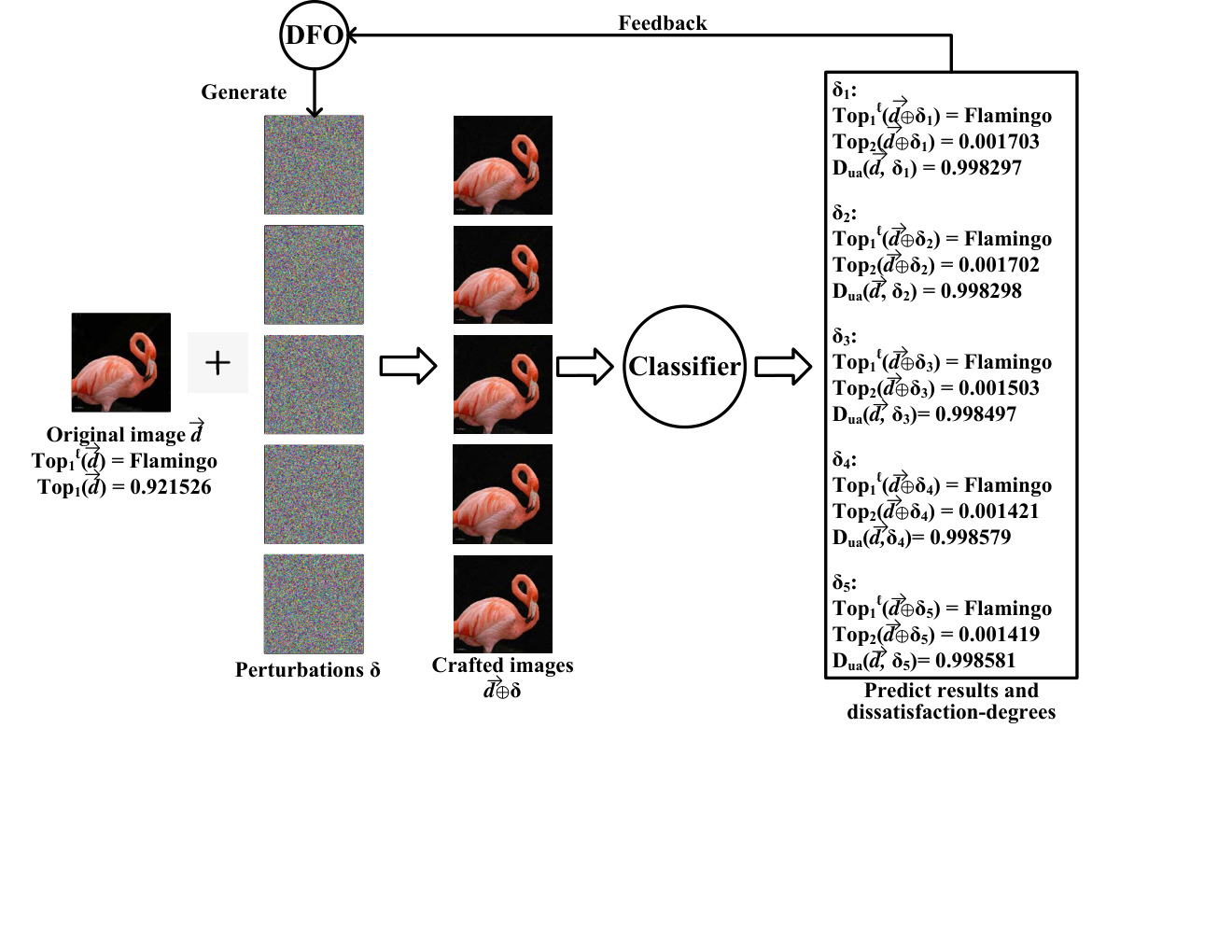
Figure 2 shows the framework of our approach named DFA, standing for Derivative-Free Attack. Given an integer image, DFA directly searches an adversarial image in a (discrete integer) search space specified by the maximum distance.
In principle, DFA first samples some perturbations from the search space and then repeats the following procedure until an integer adversarial example is found. During each iteration, DFA queries the target classifier to measure the images (perturbations added onto the input image) via a given dissatisfaction degree function which predicates how far is an image from a success attack. The perturbations is partitioned into two parts w.r.t. dissatisfaction degrees: perturbations yielding high dissatisfaction degrees and perturbations yielding low dissatisfaction degrees. The search space is refined into a small sub-space according to the partitions of perturbations. New perturbations are sampled from the refined sub-space. Together with old perturbations, a set of best-so-far perturbations is selected according to their dissatisfaction degrees. Finally, the procedure is repeated on the best-so-far perturbations which will be used to refine the sub-space again.
5.2. Formulation
We formalize the integer adversarial example searching problem as a derivative-free discrete optimization problem by defining the dissatisfaction degree functions. We first introduce some notations.
Let us fix a classifier for some image classification task and an integer number denoting the maximum distance. We denote by the vector of probabilities on the image and by the probability that the image is classified to the class . For a given integer such taht , we denote by the -th largest probability in and the class whose probability is . Obviously, .
We define the initial search space of perturbations as a discrete integer domain . Specifically, the discrete domain is a two-dimensional array such that for each coordinate , and (such that ) are integer numbers respectively denoting the lower and upper bound of the value at the coordinate . Therefore, denotes a set of perturbations such that if and only if for all coordinates . The search space will be refined into small sub-spaces by increasing lower bound or decreasing upper bound for choosing coordinates in our algorithm.
Given a perturbation , we denote by , the valid image after adding the perturbation onto the image , namely, for every coordinate :
The integer adversarial example searching problem with respect to the maximum distance is to find some perturbation such that:
- •
for untargeted attack;
- •
for targeted attack with a target class .
We solve the integer adversarial example searching problem by reduction to a derivative-free discrete optimization problem. The reduction is given by defining an optimization goal which is characterized by dissatisfaction-degree functions. We first consider the untargeted case.
The goal of untargeted attack is to find some perturbation such that . To do this, we maximize the current probability of the image being classified as the class (i.e., the current class with second largest probability, which may change w.r.t. different ) until the image is able to successfully mislead the classifier. Therefore, we define the dissatisfaction-degree function for untargeted attack, denoted by , as follows:
- •
, if ;
- •
, otherwise.
In this function, if the attack has succeeded, the perturbation is “satisfying”, then the value of the dissatisfaction-degree becomes . Otherwise, we return the distance between and the currently reported second largest probability, which is in the range of , indicating how far it is from 1. Clearly, in this case, the distance is definitely positive. To this end, our goal is to find a perturbation such that the dissatisfaction-degree is .
For targeted attack with the target class , instead of maximizing the probability of being classified as the class , we maximize the probability of the image being classified as . Hence, the dissatisfaction-degree function, denoted by , is defined as follows:
- •
, if ;
- •
, otherwise.
Now, the integer adversarial example searching problem is reduced to the minimization problem of the dissatisfaction-degree functions.
5.3. Algorithm
Instead of using heuristic search methods, e.g. genetic programming, particle swarm optimization, simulated annealing, to solve the minimization problem of the dissatisfaction-degree functions, we propose a classification model-based DFO method (shown in Algorithm 1). Different from heuristic search based methods, our method maintains a classification model during the search to distinguish “good” samples from “bad” samples. Then, the search space will be refined by learning from the samples to help to converge to the best solution.
In detail, Algorithm 1 first initializes the search space according to the given maximum distance (Line 1). Then, it randomly selects perturbations (stored as the set ) from the search space (Line 2), where denotes the sample size during each iteration and denotes the ranking threshold. Next, it computes valid images by adding the perturbations onto the source integer image and evaluates the dissatisfaction-degree (d.d.) of the these images using the dissatisfaction-degree function (Line 3). The perturbation with the smallest dissatisfaction-degree is selected from the set (Line 4). After that, Algorithm 1 repeats the following procedure.
For each iteration , if the perturbation suffices to craft an integer adversarial example, return (Lines 6-7). Otherwise, the set of perturbations is partitioned into two sets: “positive” set and “negative” set , where consists of the smallest- perturbations in terms of the dissatisfaction-degree (Lines 8-9).
Based on and , Algorithm 1 refines the search space into a small sub-space (Lines 11-34) as follows. It first randomly selects a sample from the positive set (Line 13) and randomly selects coordinates to refine (Lines 15-27). For each selected coordinate , it compares the number of perturbations in whose value is larger than the value of at the coordinate against the number of perturbations in whose value is smaller than the value of at the coordinate . If the majority of perturbations in are larger than at the coordinate , we decrease the upper bound of the search space (Lines 20-23), otherwise increase the lower bound (Lines 25-27), at the coordinate . Once coordinates have been processed, we craft a new image from by reassigning the value of each coordinate with the random integer from to (Lines 29-33). The new perturbation is added into the set . Then, the search space is reset to the original size. We remark that the refining procedure for the next sample will be conducted on the original search space to avoid over fitting.
When the search space has been refined times, we get new perturbations (i.e., set ), resulting in perturbations in the set . From them, we choose the smallest- perturbations in terms of the dissatisfaction-degree (Line 37). Algorithm 1 continues the above procedure on until an integer adversarial example is found or the number of iterations is reached.
Dimensionality reduction. Algorithm 1 depicts the main workflow of our approach which solves the integer adversarial example searching problem by a classification model-based DFO method. It can be further optimized by a dimensionality reduction technique, which reduces the search space into a lower dimensional space, to improve query efficiency. Dimensionality reduction has been adopted in recent attacks, e.g., AutoZOOM (Tu et al. 2019) and GenAttack (Alzantot et al. 2019). Instead of searching in the large search space , we can first search a perturbation in a small search space for and , and scale up to with the same size as input (i.e. the search space ) by applying resizing methods (e.g., bilinear resizing), resulting in the valid image in the original size. (Please refer to (Tu et al. 2019) and (Alzantot et al. 2019) for the more details of dimensionality reduction.) By doing so, the query efficiency of our method can be improved while maintaining the attack success rate under the constraint.
5.4. Illustrative Example
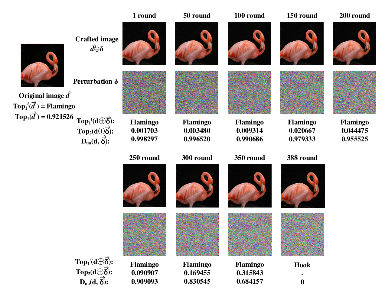
We illustrate Algorithm 1 through an example, as shown in Figure 3. The original integer image is an image from the ImageNet dataset and it is classified as the class flamingo by the target classifier Inception-v3. To launch untargeted attack using this image, we set the sample size as and the ranking threshold as . Consider the first iteration, Algorithm 1 samples perturbations from and adds them onto the original image, resulting in five new images (shown in Figure 3). Then, it computes the dissatisfaction degrees of these five new images by querying the classifier and the dissatisfaction-degree function . Among these perturbations, has the smallest dissatisfaction degree, hence is the best-so-far perturbation. After more iterations, the results are shown in Figure 4. We can see that after the -th iteration, the image with smallest dissatisfaction degree is classified as the class hook, but is visually indistinguishable from the original one.
5.5. Scenario Extension
Our framework is very reflexible and could be potentially adapted to other scenarios such as: (1) target classifiers that only output top-1 class and its probability, and (2) target classifiers that are integrated with defenses, by restricting the search space or modifying dissatisfaction-degree functions.
For instance, if the adversary only have access to the top-1 class and its probability, the dissatisfaction-degree function for untargeted attack can be adapted as follows:
- •
, if ;
- •
, otherwise.
The dissatisfaction-degree function for targeted attack could be adapted accordingly. Remark that it is different from label-only attacks in which the adversary has access to the top-1 class, but not its probability. We leave this to future work.
6. Implementation and Evaluation
We implement our classification model-based DFO method in DFA based on the framework of RACOS (Yu et al. 2016), for which we implement our new algorithm and manage to engineer to significantly improve its efficiency and scalability with lots of domain-specific optimizations. Hereafter, we report experimental results compared with state-of-the-art white-box and black-box attacks.
6.1. Dataset & Setting
Dataset. We use two standard datasets MNIST (LeCun et al. 1998) and ImageNet (Deng et al. 2009). MNIST is a dataset of handwritten digits with classes (0-9). We choose the first 200 images out of validation images of MNIST as our subjects.
We use the same 100 ImageNet images as in Section 4.3. (Recall that we randomly choose 100 classes from which we randomly choose 1 image per class that can be correctly classified by four classifiers in Keras: ResNet50, Inception-v3, VGG16 and VGG19.)
Target model. For MNIST images, we use a DNN classifier LeNet-1 from the LeNet family (Lecun et al. 1998). LeNet-1 is a popular target model for MNIST images, e.g., (Pei et al. 2017; Ma et al. 2018; Sekhon and Fleming 2019; Guo et al. 2018; Xie et al. 2019). For ImageNet images, we use a pre-trained DNN classifier Inception-v3 (Szegedy et al. 2016) which is a widely used target model for ImageNet images, e.g., (Carlini and Wagner 2017b; Chen et al. 2017; Tu et al. 2019; Ilyas et al. 2018; Alzantot et al. 2019).
| Parameter | Setting | |||||
|---|---|---|---|---|---|---|
| Max. distance | for MNIST and for ImageNet. | |||||
|
| |||||
|
| |||||
|
| |||||
|
| |||||
| Iteration Threshold |
| |||||
| Timeout Threshold |
| |||||
| Resized Space |
|
Setting. As shown in Section 4.3, the discretization problem can be avoided or alleviated by tuning input parameters for some tools, at the cost of attack efficiency or quality of adversarial examples, except for FGSM and C&W+GS. Therefore, to maximize their TSRs as done in Section 4.3, we choose proper step sizes for FGSM and enable greedy search for C&W+GS with parameters recommended by Carlini on MNIST images. For other tools, we use the parameters as in their raw papers which are already fine-tuned by the authors for effectiveness and efficiency. A discussion on turning input parameters refers to Section 4.3.2. Furthermore, some tools only provide implementations for attacking under some specific settings. If this issue happens, we may not modify their implementations as it may greatly under-estimate their effectiveness and efficiency, as pointed out by Carlini (Carlini 2019), hence some attacks are not evaluated in all settings.
We conduct both untargeted attack and targeted attack on a Linux PC running UBUNTU 16.04 LTS with Intel Xeon(R) W-2123 CPU, TITAN Xp COLLECTORS GPU and 64G RAM. Table 4 lists the other experiment settings.
| Dataset & DNN | Method | SR | TSR | GAP |
|---|---|---|---|---|
| MNIST LeNet-1 | FGSM | 97% | 97% | 0% |
| BIM | 100% | 100% | 0% | |
| C&W | 100% | 88% | 12% | |
| C&W+GS | 100% | 100% | 0% | |
| DFA | 100% | 100% | 0% | |
| ImageNet Inception-v3 | FGSM | 79% | 79% | 0% |
| BIM | 100% | 100% | 0% | |
| C&W | 100% | 68% | 32% | |
| DFA | 99% | 99% | 0% |
| Dataset & DNN | Method | SR | TSR | GAP |
| MNIST LeNet-1 | FGSM-1 | 84% | 84% | 0% |
| BIM | 100% | 100% | 0% | |
| C&W | 100% | 75% | 25% | |
| C&W+GS | 100% | 100% | 0% | |
| DFA | 100% | 100% | 0% | |
| ImageNet Inception-v3 | FGSM-1 | 9% | 9% | 0% |
| BIM | 99% | 99% | 0% | |
| C&W | 100% | 24% | 76% | |
| DFA | 96% | 96% | 0% |
6.2. Comparison with White-Box Methods
Although our method is a black-box one, we compare the performance with four well-known white-box tools: FGSM, BIM, C&W and C&W+GS, where the implementations are by their authors. Since FGSM has nearly no ability to handle targeted attack, we use one-step target class method (denoted by FGSM-1) of (Kurakin et al. 2017b), which can be regarded as the targeted version of FGSM. The maximum distances are transformed into their maximum distances accordingly.
The results are shown in Table 5 and Table 6 for untargeted and targeted attacks, respectively. Notice that C&W+GS only implements attacks for MNIST images, hence is not applied to ImageNet images.
Overall, our attack DFA achieves close to 100% attack success rates for both targeted and untargeted attacks. In terms of SR, our tool DFA outperforms FGSM/FGSM-1 and is comparable to the other tools. In terms of TSR, DFA is comparable to BIM and outperforms FGSM, FGSM-1 and C&W in most cases.
Specifically, FGSM, FGSM-1, BIM and C&W+GS do not have any gap due to the tuning of step sizes and the greedy search based algorithm. It is easy to observe that C&W has a relatively larger gap in targeted attacks on Inception-v3 in norm setting, as its TSR is only compared with SR. Thus, although C&W outperforms DFA in terms of SR, DFA outperforms C&W in most cases in terms of TSR. We remark that the gap of C&W is slightly different from the one given in Table 3, as C&W- has an input parameter which can control the confidence. By increasing , the confidence of real adversarial examples as well as the TSR of C&W- increase, and the gap can be minimized. Whereas C&W- does not have this parameter.
6.3. Comparison with Black-Box Methods
We compare DFA with well-known recent black-box methods: substitute model based attacks, ZOO, NES-PGD, FD, FD-PSO, and also three concurrent works Bandits, AutoZOOM and GenAttack, representing all the classes of existing black-box attacks (cf. Section 2), where the implementations are by their authors.
Recall that it is very difficult to tune input parameters for those tools without loss of attack efficiency or quality of adversarial examples, hence we use the parameters as in their raw papers which are already fine-tuned by the authors. When evaluating substitute model, we use FGSM/FGSM-1 and C&W methods, and use ResNet50 (He et al. 2016) as the substitute model for Inception-v3, the model in ZOO as the substitute model for LeNet-1. Since ZOO and AutoZOOM use distance, we map our maximum distances into maximum distances by considering the worst case of , namely, all the pixels are modified by the maximum distance. For instance, the distance 10 is approximated by distance for images. Remark that this is not a rigorous mapping, ZOO and AutoZOOM under would be easier to find an adversarial example, as the corresponding distances are less restricted.
The results of untargeted and targeted attacks are given in Table 7 and Table 8. We can see that our attack DFA achieves close to 100% attack success rates for both targeted and untargeted attacks and outperforms all the other tools in terms of TSR no matter targeted or untargeted attacks. In terms of SR, our tool is also comparable (or better) to the other tools. One may notice that substitute models perform poorly. This may due to the difference between training data and architectures of the substitute model and the target model, as the larger gap between the substitute model and the target model is, the less effective of transferability of adversarial samples is.
| Dataset & DNN | Method | SR | TSR | GAP |
| MNIST LeNet-1 | SModel+C&W | 2.5% | 2.5% | 0% |
| SModel+FGSM | 20% | 20% | 0% | |
| FD | 94.5% | 94.5% | 0% | |
| FD-PSO | 46.5% | 46.5% | 0% | |
| DFA | 100% | 100% | 0% | |
| ImageNet Inception-v3 | SModel+C&W | 6% | 6% | 0% |
| SModel+FGSM | 38% | 38% | 0% | |
| ZOO | 89% | 5% | 94.3% | |
| AutoZOOM | 100% | 57% | 43% | |
| NES-PGD | 100% | 77% | 23% | |
| Bandits | 100% | 12% | 88% | |
| GenAttack | 100% | 93% | 7% | |
| DFA | 99% | 99% | 0% |
| Dataset & DNN | Method | SR | TSR | GAP |
| MNIST LeNet-1 | SModel+C&W | 1.5% | 1.5% | 0% |
| SModel+FGSM-1 | 5% | 5% | 0% | |
| FD | 72% | 72% | 0% | |
| FD-PSO | 6.5% | 6.5% | 0% | |
| DFA | 100% | 100% | 0% | |
| ImageNet Inception-v3 | SModel+C&W | 1% | 1% | 0% |
| SModel+FGSM-1 | 2% | 2% | 0% | |
| ZOO | 69% | 5% | 92.7% | |
| AutoZOOM | 95% | 43% | 54.7% | |
| NES-PGD | 100% | 47% | 53% | |
| GenAttack | 100% | 84% | 16% | |
| DFA | 96% | 96% | 0% |
| Dataset & DNN | Method | Untargeted | Targeted | ||
| Query | MSE | Query | MSE | ||
| MNIST LeNet-1 | FD | 1568 | 3.4e-2 | 1568 | 3.5e-2 |
| FD-PSO | 10000 | 2.5e-2 | 10000 | 2.5e-2 | |
| DFA | 817 | 3.7e-2 | 1593 | 5.1e-2 | |
| ImageNet Inception-v3 | ZOO | 85368 | 1.7e-5 | 203683 | 3.6e-5 |
| AutoZOOM | 2224 | 9.2e-4 | 14322 | 1.2e-3 | |
| NES-PGD | 4741 | 8.4e-4 | 13421 | 9.0e-4 | |
| Bandits | 4595 | 1.4e-3 | - | - | |
| GenAttack | 4008 | 6.3e-4 | 12369 | 9.2e-4 | |
| DFA | 4746 | 2.6e-4 | 12740 | 3.4e-4 | |
6.4. Query Comparison.
In many black-box scenarios, the attacker has a limited number of queries to the classifier. Therefore, we report the average number of queries of the black-box attacks in Table 9, where substitute model based attack is excluded due to its low SR. We remark that ZOO is regarded as baseline, the others are state-of-the-art query-efficient tools.
On attack against Inception-v3, our tool DFA outperforms all the other tools for targeted attacks, except for GenAttack, which is slightly better than DFA. For untargeted attacks, our tool DFA outperforms the baseline tool ZOO and comparable to other tools. Recall that our tool DFA outperforms all these tools in terms of TSR.
We remark that ZOO and AutoZOOM are tested under the distance 20, which is less restricted than the distance 10 used for the other tools. Indeed, in untargeted attack setting, the average distance of our tool is 8.33. Whereas the average query times of AutoZOOM becomes 4971 (worse than ours) if .
On attack against LeNet-1, our tool DFA outperforms both of them in almost all cases, exception that FD uses less query times than DFA for targeted attacks. Note that our tool DFA achieves higher attack success attack rate than FD and FD-PSO in terms of both SR/TSR. One may notice that the query times of FD and FD-PSO are same between untargeted and targeted attacks. This is due to the implementations of FD and FD-PSO (confirmed by some authors of (Bhagoji et al. 2018)).
Furthermore, we also report the average Mean Square Error (MSE) of the adversarial examples in Table 9. We can observe that our tool DFA outperforms most of the other tools on attacks against Inception-v3. FD and FD-PSO are slightly better than DFA on attacks against LeNet-1, at the same order of magnitude. ZOO outperforms all the other tools in terms of MSE against Inception-v3, but at the cost of huge number of query times.
6.5. Attack Classifiers with Defense
To show the effectiveness of our approach, we use our tool to attack the HGD defense (Liao et al. 2018), which won the first place of NIPS 2017 competition on defense against adversarial attacks. HGD defense is a typical denoising based defensing methods for image classification. The whole classification system is an ensemble of 4 independent models and their denoiser (ResNet, ResNext, InceptionV3, inceptionResNetV2). We conduct untargeted attacks against this model using the same 100 ImageNet images and parameters as previously, exception that the distance is according to the NIPS 2017 competition. Our tool achieves TSR in the experiments, indicating the effectiveness of DFA. This benefits from the advantage of our classification model-based derivative-free optimization method, which does not rely on the gradient of the objective function, but instead, learns from samples of the search space, hence suitable for attack systems that are non-differentiable or even unknown but only testable.
MNIST Adversarial Examples Challenge (Lab 2019) is another widely recognized attack problem. It uses adversarial training for defensing. We use the same 200 MNIST images as previously on the attack of this problem. Our tool DFA achieves TSR, the same as the current best white-box attack “interval attacks”, which is publicly reported on the webpage of the challenge. The images on which the attacks succeed by both methods are exactly same, and the time costs of both tools are also similar.
7. Conclusion and Future Work
We conducted the first comprehensive study of 35 methods and 20 open source tools for crafting adversarial examples, in an attempt to understand the impacts of the discretization problem. Our study revealed that most of these methods and tools are affected by this problem and researchers should pay more attention when designing adversarial example attacks and measuring attack success rate. We also proposed strategies to avoid or alleviate the discretization problem, which can improve TSR of some tools, at the cost of attack efficiency or imperceptibility of adversarial examples.
We proposed a black-box method by designing a classification model-based derivative-free optimization method. Our method directly crafts adversarial examples in discrete integer domains, hence does not have the discretization problem and is able to attack a wide range of classifiers including non-differentiable ones. Our attack method requires access to the probability distribution of classes for each test input and does not rely on the gradient of the objective function, but instead, learns from samples of the search space. We implemented our method into tool DFA, and conducted an intensive set of experiments on MNIST and ImageNet in both untargeted and targeted scenarios. The experimental results show that our method achieved close to 100% attack success rate, comparable to the white-box methods (FGSM, BIM and C&W) and outperformed the state-of-the-art black-box methods. Moreover, our method achieved success rate on the winner of NIPS 2017 competition on defense, and achieved the same result as the best white-box attack in MNIST Challenge. Our results suggest that classification model-based derivative-free discrete optimization opens up a promising research direction into effective black-box attacks. Our method could serve as a test for designing robust networks.
In future, we plan to lift our generic method to other neural network based systems such as face recognition systems (Sharif et al. 2016) and speech recognition (Yuan et al. 2018; Carlini et al. 2016). It is also worth investigating how to intergrade gradient estimation techniques into our sampling. This may improves query efficiency of our method.
Acknowledgements.
This work is supported by the National Natural Science Foundation of China (NSFC) Grants (Nos. 61532019, 61761136011 and 61572249),References
- (1)
- iss (2019a) 2019a. https://github.com/peikexin9/deepxplore/issues/20.
- iss (2019b) 2019b. https://github.com/bethgelab/foolbox/issues/264.
- iss (2019c) 2019c. https://github.com/tensorflow/cleverhans/issues/265.
- Alzantot et al. (2019) Moustafa Alzantot, Yash Sharma, Supriyo Chakraborty, Huan Zhang, Cho-Jui Hsieh, and Mani B. Srivastava. 2019. GenAttack: practical black-box attacks with gradient-free optimization. In Proceedings of the Genetic and Evolutionary Computation Conference. 1111–1119.
- Andor et al. (2016) Daniel Andor, Chris Alberti, David Weiss, Aliaksei Severyn, Alessandro Presta, Kuzman Ganchev, Slav Petrov, and Michael Collins. 2016. Globally Normalized Transition-Based Neural Networks. In Proceedings of the 54th Annual Meeting of the Association for Computational Linguistics.
- Apollo (2018) Apollo. 2018. An open, reliable and secure software platform for autonomous driving systems. http://apollo.auto.
- Athalye et al. (2018) Anish Athalye, Logan Engstrom, Andrew Ilyas, and Kevin Kwok. 2018. Synthesizing Robust Adversarial Examples. In Proceedings of the 35th International Conference on Machine Learning. 284–293.
- Bastani et al. (2016) Osbert Bastani, Yani Ioannou, Leonidas Lampropoulos, Dimitrios Vytiniotis, Aditya V. Nori, and Antonio Criminisi. 2016. Measuring Neural Net Robustness with Constraints. In NIPS. 2613–2621.
- Bhagoji et al. (2017) Arjun Nitin Bhagoji, Warren He, Bo Li, and Dawn Song. 2017. Exploring the Space of Black-box Attacks on Deep Neural Networks. CoRR abs/1712.09491 (2017).
- Bhagoji et al. (2018) Arjun Nitin Bhagoji, Warren He, Bo Li, and Dawn Song. 2018. Practical Black-Box Attacks on Deep Neural Networks Using Efficient Query Mechanisms. In Proceedings of the 15th European Conference on Computer Vision (ECCV). 158–174.
- Brendel et al. (2018) Wieland Brendel, Jonas Rauber, and Matthias Bethge. 2018. Decision-Based Adversarial Attacks: Reliable Attacks Against Black-Box Machine Learning Models. In International Conference on Learning Representations.
- Brendel et al. (2019) Wieland Brendel, Jonas Rauber, Matthias Kümmerer, Ivan Ustyuzhaninov, and Matthias Bethge. 2019. Accurate, reliable and fast robustness evaluation. CoRR abs/1907.01003 (2019).
- Brown et al. (2017) Tom B. Brown, Dandelion Mané, Aurko Roy, Martín Abadi, and Justin Gilmer. 2017. Adversarial Patch. CoRR abs/1712.09665 (2017).
- Carlini (2019) Nicholas Carlini. 2019. A critique of the DeepSec Platform for Security Analysis of Deep Learning Models. CoRR abs/1905.07112 (2019).
- Carlini et al. (2016) Nicholas Carlini, Pratyush Mishra, Tavish Vaidya, Yuankai Zhang, Micah Sherr, Clay Shields, David A. Wagner, and Wenchao Zhou. 2016. Hidden Voice Commands. In 25th USENIX Security Symposium. 513–530.
- Carlini and Wagner (2017a) Nicholas Carlini and David A. Wagner. 2017a. Adversarial Examples Are Not Easily Detected: Bypassing Ten Detection Methods. In Proceedings of the 10th ACM Workshop on Artificial Intelligence and Security. 3–14.
- Carlini and Wagner (2017b) Nicholas Carlini and David A. Wagner. 2017b. Towards Evaluating the Robustness of Neural Networks. In 2017 IEEE Symposium on Security and Privacy. 39–57.
- Chen et al. (2018b) Pin-Yu Chen, Yash Sharma, Huan Zhang, Jinfeng Yi, and Cho-Jui Hsieh. 2018b. EAD: Elastic-Net Attacks to Deep Neural Networks via Adversarial Examples. In Proceedings of the Thirty-Second AAAI Conference on Artificial Intelligence (AAAI). 10–17.
- Chen et al. (2017) Pin-Yu Chen, Huan Zhang, Yash Sharma, Jinfeng Yi, and Cho-Jui Hsieh. 2017. ZOO: Zeroth Order Optimization Based Black-box Attacks to Deep Neural Networks without Training Substitute Models. In Proceedings of the 10th ACM Workshop on Artificial Intelligence and Security. 15–26.
- Chen et al. (2018a) Shang-Tse Chen, Cory Cornelius, Jason Martin, and Duen Horng Chau. 2018a. ShapeShifter: Robust Physical Adversarial Attack on Faster R-CNN Object Detector. ArXiv abs/1804.05810 (2018).
- Cheng et al. (2018) Minhao Cheng, Thong Le, Pin-Yu Chen, Jinfeng Yi, Huan Zhang, and Cho-Jui Hsieh. 2018. Query-Efficient Hard-label Black-box Attack: An Optimization-based Approach. CoRR abs/1807.04457 (2018).
- Chollet et al. (2015) François Chollet et al. 2015. Keras. https://keras.io.
- Ciresan et al. (2012) Dan C. Ciresan, Alessandro Giusti, Luca Maria Gambardella, and Jürgen Schmidhuber. 2012. Deep Neural Networks Segment Neuronal Membranes in Electron Microscopy Images. In Proceedings of the 26th Annual Conference on Neural Information Processing Systems. 2852–2860.
- Co et al. (2019) Kenneth T Co, Luis Muñoz-González, Sixte de Maupeou, and Emil C Lupu. 2019. Procedural Noise Adversarial Examples for Black-Box Attacks on Deep Convolutional Networks. In CCS 2019 (accepted).
- Coates et al. (2011) Adam Coates, Andrew Y. Ng, and Honglak Lee. 2011. An Analysis of Single-Layer Networks in Unsupervised Feature Learning. In Proceedings of the Fourteenth International Conference on Artificial Intelligence and Statistics. 215–223.
- Dalvi et al. (2004) Nilesh N. Dalvi, Pedro M. Domingos, Mausam, Sumit K. Sanghai, and Deepak Verma. 2004. Adversarial classification. In Proceedings of the Tenth ACM SIGKDD International Conference on Knowledge Discovery and Data Mining. 99–108.
- Demontis et al. (2017) Ambra Demontis, Marco Melis, Battista Biggio, Davide Maiorca, Daniel Arp, Konrad Rieck, Igino Corona, Giorgio Giacinto, and Fabio Roli. 2017. Yes, machine learning can be more secure! a case study on android malware detection. IEEE Transactions on Dependable and Secure Computing (2017).
- Deng et al. (2009) Jia Deng, Wei Dong, Richard Socher, Li-Jia Li, Kai Li, and Fei-Fei Li. 2009. ImageNet: A large-scale hierarchical image database. In 2009 IEEE Computer Society Conference on Computer Vision and Pattern Recognition (CVPR). 248–255.
- Dong et al. (2018) Yinpeng Dong, Fangzhou Liao, Tianyu Pang, Hang Su, Jun Zhu, Xiaolin Hu, and Jianguo Li. 2018. Boosting Adversarial Attacks With Momentum. In Proceedings of 2018 IEEE Conference on Computer Vision and Pattern Recognition. 9185–9193.
- Dvijotham et al. (2018) Krishnamurthy Dvijotham, Robert Stanforth, Sven Gowal, Timothy A. Mann, and Pushmeet Kohli. 2018. A Dual Approach to Scalable Verification of Deep Networks. CoRR abs/1803.06567 (2018).
- Ehlers (2017) Rüdiger Ehlers. 2017. Formal Verification of Piece-Wise Linear Feed-Forward Neural Networks. In Proceedings of the 15th International Symposium on Automated Technology for Verification and Analysis. 269–286.
- Eykholt et al. (2018a) Kevin Eykholt, Ivan Evtimov, Earlence Fernandes, Bo Li, Amir Rahmati, Florian Tramèr, Atul Prakash, Tadayoshi Kohno, and Dawn Song. 2018a. Physical Adversarial Examples for Object Detectors. In 12th USENIX Workshop on Offensive Technologies.
- Eykholt et al. (2018b) Kevin Eykholt, Ivan Evtimov, Earlence Fernandes, Bo Li, Amir Rahmati, Chaowei Xiao, Atul Prakash, Tadayoshi Kohno, and Dawn Song. 2018b. Robust Physical-World Attacks on Deep Learning Visual Classification. In Proceedings of 2018 IEEE Conference on Computer Vision and Pattern Recognition. 1625–1634.
- Eykholt et al. (2017) Kevin Eykholt, Ivan Evtimov, Earlence Fernandes, Bo Li, Dawn Song, Tadayoshi Kohno, Amir Rahmati, Atul Prakash, and Florian Tramèr. 2017. Note on Attacking Object Detectors with Adversarial Stickers. CoRR abs/1712.08062 (2017).
- Gehr et al. (2018) Timon Gehr, Matthew Mirman, Dana Drachsler-Cohen, Petar Tsankov, Swarat Chaudhuri, and Martin T. Vechev. 2018. AI2: Safety and Robustness Certification of Neural Networks with Abstract Interpretation. In Proceedings of the 2018 IEEE Symposium on Security and Privacy. 3–18.
- Goodfellow et al. (2014) Ian Goodfellow, Jonathon Shlens, and Christian Szegedy. 2014. Explaining and harnessing adversarial examples. In International Conference on Learning Representations.
- Goodfellow et al. (2016) Ian J. Goodfellow, Yoshua Bengio, and Aaron C. Courville. 2016. Deep Learning. MIT Press.
- Goodfellow et al. (2013) Ian J. Goodfellow, David Warde-Farley, Mehdi Mirza, Aaron C. Courville, and Yoshua Bengio. 2013. Maxout Networks. In Proceedings of the 30th International Conference on Machine Learning. 1319–1327.
- Gopinath et al. (2018) Divya Gopinath, Guy Katz, Corina S. Pasareanu, and Clark Barrett. 2018. DeepSafe: A Data-Driven Approach for Assessing Robustness of Neural Networks. In Proceedings of the 16th International Symposium on Automated Technology for Verification and Analysis. 3–19.
- Grosse et al. (2017) Kathrin Grosse, Nicolas Papernot, Praveen Manoharan, Michael Backes, and Patrick McDaniel. 2017. Adversarial examples for malware detection. In European Symposium on Research in Computer Security. Springer, 62–79.
- Guo et al. (2018) Jianmin Guo, Yu Jiang, Yue Zhao, Quan Chen, and Jiaguang Sun. 2018. DLFuzz: differential fuzzing testing of deep learning systems. In Proceedings of the 2018 ACM Joint Meeting on European Software Engineering Conference and Symposium on the Foundations of Software Engineering (ESEC/SIGSOFT). 739–743.
- He et al. (2016) Kaiming He, Xiangyu Zhang, Shaoqing Ren, and Jian Sun. 2016. Deep Residual Learning for Image Recognition. In 2016 IEEE Conference on Computer Vision and Pattern Recognition (CVPR). 770–778.
- He et al. (2018) Warren He, Bo Li, and Dawn Song. 2018. Decision boundary analysis of adversarial examples. In Proceedings of International Conference on Learning Representations.
- Hinton et al. (2012) G. Hinton, L. Deng, D. Yu, G. E. Dahl, A. Mohamed, N. Jaitly, A. Senior, V. Vanhoucke, P. Nguyen, T. N. Sainath, and B. Kingsbury. 2012. Deep Neural Networks for Acoustic Modeling in Speech Recognition: The Shared Views of Four Research Groups. IEEE Signal Process. Mag. 29, 6 (2012), 82–97.
- Holley (2018) Peter Holley. 2018. Texas becomes the latest state to get a self-driving car service. https://www.washingtonpost.com/news/innovations/wp/2018/05/07/texas-becomes-the-latest-state-to-get-a-self-driving-car-service.
- Hosseini et al. (2017) Hossein Hosseini, Baicen Xiao, and Radha Poovendran. 2017. Google’s Cloud Vision API is Not Robust to Noise. In Proceedings of the 16th IEEE International Conference on Machine Learning and Applications. 101–105.
- Huang et al. (2017b) Gao Huang, Zhuang Liu, Laurens van der Maaten, and Kilian Q. Weinberger. 2017b. Densely Connected Convolutional Networks. In 2017 IEEE Conference on Computer Vision and Pattern Recognition. 2261–2269.
- Huang et al. (2017a) Xiaowei Huang, Marta Kwiatkowska, Sen Wang, and Min Wu. 2017a. Safety Verification of Deep Neural Networks. In Proceedings of the 29th International Conference on Computer Aided Verification. 3–29.
- Ilyas et al. (2017) Andrew Ilyas, Logan Engstrom, Anish Athalye, and Jessy Lin. 2017. Query-Efficient Black-box Adversarial Examples. arXiv preprint arXiv:1712.07113 (2017).
- Ilyas et al. (2018) Andrew Ilyas, Logan Engstrom, Anish Athalye, and Jessy Lin. 2018. Black-box Adversarial Attacks with Limited Queries and Information. In Proceedings of the 35th International Conference on Machine Learning. 2142–2151.
- Ilyas et al. (2019) Andrew Ilyas, Logan Engstrom, and Aleksander Madry. 2019. Prior Convictions: Black-box Adversarial Attacks with Bandits and Priors. In 7th International Conference on Learning Representations (ICLR).
- Jan et al. (2019) Steve T. K. Jan, Joseph Messou, Yen-Chen Lin, Jia-Bin Huang, and Gang Wang. 2019. Connecting the Digital and Physical World: Improving the Robustness of Adversarial Attacks. In The Thirty-Third AAAI Conference on Artificial Intelligence. 962–969.
- Karpathy et al. (2014) Andrej Karpathy, George Toderici, Sanketh Shetty, Thomas Leung, Rahul Sukthankar, and Fei-Fei Li. 2014. Large-Scale Video Classification with Convolutional Neural Networks. In Proceedings of 2014 IEEE Conference on Computer Vision and Pattern Recognition. 1725–1732.
- Katz et al. (2017) Guy Katz, Clark W. Barrett, David L. Dill, Kyle Julian, and Mykel J. Kochenderfer. 2017. Reluplex: An Efficient SMT Solver for Verifying Deep Neural Networks. In Proceedings of the 29th International Conference on Computer Aided Verification. 97–117.
- Kos et al. (2018) Jernej Kos, Ian Fischer, and Dawn Song. 2018. Adversarial Examples for Generative Models. In Proceedings of 2018 IEEE Security and Privacy Workshops. 36–42.
- Krizhevsky et al. (2017) Alex Krizhevsky, Ilya Sutskever, and Geoffrey E. Hinton. 2017. ImageNet classification with deep convolutional neural networks. Commun. ACM 60, 6 (2017), 84–90.
- Kurakin et al. (2017a) Alexey Kurakin, Ian Goodfellow, and Samy Bengio. 2017a. Adversarial examples in the physical world. In Proceedings of International Conference on Learning Representations.
- Kurakin et al. (2017b) Alexey Kurakin, Ian J. Goodfellow, and Samy Bengio. 2017b. Adversarial Machine Learning at Scale. In Proceedings of the 5th International Conference on Learning Representations (ICLR).
- Lab (2019) Madry Lab. 2019. MNIST Adversarial Examples Challenge. https://github.com/MadryLab/mnist_challenge.
- Lecun et al. (1998) Y. Lecun, L. Bottou, Y. Bengio, and P. Haffner. 1998. Gradient-based learning applied to document recognition. Proc. IEEE 86, 11 (1998), 2278–2324.
- LeCun et al. (1998) Yann LeCun, Corinna Cortes, and Christopher JC Burges. 1998. The mnist database of handwritten digits.
- Levine et al. (2018) Sergey Levine, Peter Pastor, Alex Krizhevsky, Julian Ibarz, and Deirdre Quillen. 2018. Learning hand-eye coordination for robotic grasping with deep learning and large-scale data collection. I. J. Robotics Res. 37, 4-5 (2018), 421–436.
- Li and Vorobeychik (2014) Bo Li and Yevgeniy Vorobeychik. 2014. Feature Cross-Substitution in Adversarial Classification. In Proceedings of Advances in Neural Information Processing Systems. 2087–2095.
- Liao et al. (2018) Fangzhou Liao, Ming Liang, Yinpeng Dong, Tianyu Pang, Xiaolin Hu, and Jun Zhu. 2018. Defense Against Adversarial Attacks Using High-Level Representation Guided Denoiser. In 2018 IEEE Conference on Computer Vision and Pattern Recognition, CVPR. 1778–1787.
- Liu et al. (2017) Yanpei Liu, Xinyun Chen, Chang Liu, and Dawn Song. 2017. Delving into Transferable Adversarial Examples and Black-box Attacks. In Proceedings of the 5th International Conference on Learning Representations.
- Lowd and Meek (2005) Daniel Lowd and Christopher Meek. 2005. Good Word Attacks on Statistical Spam Filters.. In CEAS, Vol. 2005.
- Lu et al. (2017a) Jiajun Lu, Hussein Sibai, and Evan Fabry. 2017a. Adversarial Examples that Fool Detectors. CoRR abs/1712.02494 (2017).
- Lu et al. (2017b) Jiajun Lu, Hussein Sibai, Evan Fabry, and David A. Forsyth. 2017b. NO Need to Worry about Adversarial Examples in Object Detection in Autonomous Vehicles. CoRR abs/1707.03501 (2017).
- Ma et al. (2018) Lei Ma, Felix Juefei-Xu, Fuyuan Zhang, Jiyuan Sun, Minhui Xue, Bo Li, Chunyang Chen, Ting Su, Li Li, Yang Liu, Jianjun Zhao, and Yadong Wang. 2018. DeepGauge: multi-granularity testing criteria for deep learning systems. In Proceedings of the 33rd ACM/IEEE International Conference on Automated Software Engineering. 120–131.
- Madry et al. (2018) Aleksander Madry, Aleksandar Makelov, Ludwig Schmidt, Dimitris Tsipras, and Adrian Vladu. 2018. Towards Deep Learning Models Resistant to Adversarial Attacks. In Proceedings of International Conference on Learning Representations.
- Maiorca et al. (2013) Davide Maiorca, Igino Corona, and Giorgio Giacinto. 2013. Looking at the bag is not enough to find the bomb: an evasion of structural methods for malicious pdf files detection. In Proceedings of the 8th ACM SIGSAC symposium on Information, computer and communications security. ACM, 119–130.
- Moosavi-Dezfooli et al. (2016) Seyed-Mohsen Moosavi-Dezfooli, Alhussein Fawzi, and Pascal Frossard. 2016. DeepFool: A Simple and Accurate Method to Fool Deep Neural Networks. In Proceedings of 2016 IEEE Conference on Computer Vision and Pattern Recognition. 2574–2582.
- Moosavi-Dezfooli et al. (2017) Seyed-Mohsen Moosavi-Dezfooli, Alhussein Fawzi, Omar Fawzi, and Pascal Frossard. 2017. Universal Adversarial Perturbations. In Proceedings of 2017 IEEE Conference on Computer Vision and Pattern Recognition. 86–94.
- Narodytska and Kasiviswanathan (2017) Nina Narodytska and Shiva Prasad Kasiviswanathan. 2017. Simple Black-Box Adversarial Attacks on Deep Neural Networks. In Proceedings of the 2017 IEEE Conference on Computer Vision and Pattern Recognition Workshops. 1310–1318.
- Nguyen et al. (2015) Anh Mai Nguyen, Jason Yosinski, and Jeff Clune. 2015. Deep neural networks are easily fooled: High confidence predictions for unrecognizable images. In Proceedings of 2015 IEEE Conference on Computer Vision and Pattern Recognition. 427–436.
- Papernot et al. (2016a) Nicolas Papernot, Patrick D. McDaniel, and Ian J. Goodfellow. 2016a. Transferability in Machine Learning: from Phenomena to Black-Box Attacks using Adversarial Samples. CoRR abs/1605.07277 (2016).
- Papernot et al. (2017) Nicolas Papernot, Patrick D. McDaniel, Ian J. Goodfellow, Somesh Jha, Z. Berkay Celik, and Ananthram Swami. 2017. Practical Black-Box Attacks against Machine Learning. In Proceedings of the 2017 ACM on Asia Conference on Computer and Communications Security. 506–519.
- Papernot et al. (2016b) Nicolas Papernot, Patrick D. McDaniel, Somesh Jha, Matt Fredrikson, Z. Berkay Celik, and Ananthram Swami. 2016b. The Limitations of Deep Learning in Adversarial Settings. In Proceedings of IEEE European Symposium on Security and Privacy. 372–387.
- Parag et al. (2015) Toufiq Parag, Dan C. Ciresan, and Alessandro Giusti. 2015. Efficient Classifier Training to Minimize False Merges in Electron Microscopy Segmentation. In Proceedings of 2015 IEEE International Conference on Computer Vision. 657–665.
- Pei et al. (2017) Kexin Pei, Yinzhi Cao, Junfeng Yang, and Suman Jana. 2017. DeepXplore: Automated Whitebox Testing of Deep Learning Systems. In Proceedings of the 26th Symposium on Operating Systems Principles. 1–18.
- Pennington et al. (2014) Jeffrey Pennington, Richard Socher, and Christopher D. Manning. 2014. Glove: Global Vectors for Word Representation. In Proceedings of the 2014 Conference on Empirical Methods in Natural Language Processing. 1532–1543.
- Pulina and Tacchella (2010) Luca Pulina and Armando Tacchella. 2010. An Abstraction-Refinement Approach to Verification of Artificial Neural Networks. In Proceedings of the 22nd International Conference on Computer Aided Verification (CAV). 243–257.
- Rauber et al. (2017) Jonas Rauber, Wieland Brendel, and Matthias Bethge. 2017. Foolbox: A Python toolbox to benchmark the robustness of machine learning models. arXiv preprint arXiv:1707.04131 (2017).
- Rosa et al. (2018) L. D. L. Rosa, S. Kilgallon, T. Vanderbruggen, and J. Cavazos. 2018. Efficient Characterization and Classification of Malware Using Deep Learning. In 2018 Resilience Week (RWS). 77–83.
- Ruan et al. (2018) Wenjie Ruan, Xiaowei Huang, and Marta Kwiatkowska. 2018. Reachability Analysis of Deep Neural Networks with Provable Guarantees. In Proceedings of the Twenty-Seventh International Joint Conference on Artificial Intelligence. 2651–2659.
- Salimans et al. (2017) Tim Salimans, Jonathan Ho, Xi Chen, and Ilya Sutskever. 2017. Evolution Strategies as a Scalable Alternative to Reinforcement Learning. CoRR abs/1703.03864 (2017). arXiv:1703.03864 http://arxiv.org/abs/1703.03864
- Sekhon and Fleming (2019) Jasmine Sekhon and Cody Fleming. 2019. Towards improved testing for deep learning. In Proceedings of the 41st International Conference on Software Engineering: New Ideas and Emerging Results (ICSE). 85–88.
- Sharif et al. (2016) Mahmood Sharif, Sruti Bhagavatula, Lujo Bauer, and Michael K. Reiter. 2016. Accessorize to a Crime: Real and Stealthy Attacks on State-of-the-Art Face Recognition. In Proceedings of the 2016 ACM SIGSAC Conference on Computer and Communications Security. 1528–1540.
- Shen et al. (2017) Dinggang Shen, Guorong Wu, , and Heung-Il Suk. 2017. Deep learning in medical image analysis. Annual Review of Biomedical Engineering 19 (2017), 221–248.
- Shi et al. (2019) Yucheng Shi, Siyu Wang, and Yahong Han. 2019. Curls & Whey: Boosting Black-Box Adversarial Attacks. In Computer Vision and Pattern Recognition (CVPR), 2019.
- Shin et al. (2015) Eui Chul Richard Shin, Dawn Song, and Reza Moazzezi. 2015. Recognizing Functions in Binaries with Neural Networks. In Proceedings of the 24th USENIX Security Symposium, USENIX Security. 611–626.
- Singh et al. (2018) Gagandeep Singh, Timon Gehr, Matthew Mirman, Markus Püschel, and Martin T. Vechev. 2018. Fast and Effective Robustness Certification. In Advances in Neural Information Processing Systems. 10825–10836.
- Singh et al. (2019) Gagandeep Singh, Timon Gehr, Markus Püschel, and Martin Vechev. 2019. An Abstract Domain for Certifying Neural Networks. In POPL.
- Sitawarin et al. (2018) Chawin Sitawarin, Arjun Nitin Bhagoji, Arsalan Mosenia, Mung Chiang, and Prateek Mittal. 2018. DARTS: Deceiving Autonomous Cars with Toxic Signs. CoRR abs/1802.06430 (2018).
- Song et al. (2018) Wei Song, Heng Yin, Chang Liu, and Dawn Song. 2018. DeepMem: Learning Graph Neural Network Models for Fast and Robust Memory Forensic Analysis. In Proceedings of the 2018 ACM SIGSAC Conference on Computer and Communications Security. 606–618.
- Srndic and Laskov (2014) Nedim Srndic and Pavel Laskov. 2014. Practical Evasion of a Learning-Based Classifier: A Case Study. In 2014 IEEE Symposium on Security and Privacy. 197–211.
- Su et al. (2019) J. Su, D. V. Vargas, and K. Sakurai. 2019. One Pixel Attack for Fooling Deep Neural Networks. IEEE Transactions on Evolutionary Computation (2019).
- Sun et al. (2018a) Youcheng Sun, Xiaowei Huang, and Daniel Kroening. 2018a. Testing Deep Neural Networks. CoRR abs/1803.04792 (2018).
- Sun et al. (2018b) Youcheng Sun, Min Wu, Wenjie Ruan, Xiaowei Huang, Marta Kwiatkowska, and Daniel Kroening. 2018b. Concolic testing for deep neural networks. In Proceedings of the 33rd ACM/IEEE International Conference on Automated Software Engineerin. 109–119.
- Szegedy et al. (2016) Christian Szegedy, Vincent Vanhoucke, Sergey Ioffe, Jonathon Shlens, and Zbigniew Wojna. 2016. Rethinking the Inception Architecture for Computer Vision. In 2016 IEEE Conference on Computer Vision and Pattern Recognition, (CVPR). 2818–2826.
- Szegedy et al. (2014) Christian Szegedy, Wojciech Zaremba, Ilya Sutskever, Joan Bruna, Dumitru Erhan, Ian Goodfellow, and Rob Fergus. 2014. Intriguing properties of neural networks. In Proceedings of International Conference on Learning Representations.
- Tabacof and Valle (2016) Pedro Tabacof and Eduardo Valle. 2016. Exploring the space of adversarial images. In 2016 International Joint Conference on Neural Networks, IJCNN 2016, Vancouver, BC, Canada, July 24-29, 2016. IEEE, 426–433. https://doi.org/10.1109/IJCNN.2016.7727230
- Tjeng et al. (2019) Vincent Tjeng, Kai Xiao, and Russ Tedrake. 2019. Evaluating Robustness Of Neural Networks With Mixed Integer Programming. ICLR.
- Tu et al. (2019) Chun-Chen Tu, Pai-Shun Ting, Pin-Yu Chen, Sijia Liu, Huan Zhang, Jinfeng Yi, Cho-Jui Hsieh, and Shin-Ming Cheng. 2019. AutoZOOM: Autoencoder-Based Zeroth Order Optimization Method for Attacking Black-Box Neural Networks. In The Thirty-Third AAAI Conference on Artificial Intelligence. 742–749.
- Wang et al. (2018) Shiqi Wang, Kexin Pei, Justin Whitehouse, Junfeng Yang, and Suman Jana. 2018. Formal Security Analysis of Neural Networks using Symbolic Intervals. In Proceedings of the 27th USENIX Security Symposium on Security. 1599–1614.
- Waymo (2009) Waymo. 2009. A self-driving technology development company. https://waymo.com/.
- Wicker et al. (2018) Matthew Wicker, Xiaowei Huang, and Marta Kwiatkowska. 2018. Feature-Guided Black-Box Safety Testing of Deep Neural Networks. In Proceedings of the 24th International Conference on Tools and Algorithms for the Construction and Analysis of Systems. 408–426.
- Wierstra et al. (2014) Daan Wierstra, Tom Schaul, Tobias Glasmachers, Yi Sun, Jan Peters, and Jürgen Schmidhuber. 2014. Natural evolution strategies. Journal of Machine Learning Research 15, 1 (2014), 949–980.
- Xiao et al. (2018) Chaowei Xiao, Jun-Yan Zhu, Bo Li, Warren He, Mingyan Liu, and Dawn Song. 2018. Spatially Transformed Adversarial Examples. In International Conference on Learning Representations.
- Xie et al. (2019) Xiaofei Xie, Lei Ma, Felix Juefei-Xu, Minhui Xue, Hongxu Chen, Yang Liu, Jianjun Zhao, Bo Li, Jianxiong Yin, and Simon See. 2019. DeepHunter: a coverage-guided fuzz testing framework for deep neural networks. In Proceedings of the 28th ACM SIGSOFT International Symposium on Software Testing and Analysis (ISSTA). 146–157.
- Xu et al. (2014) Li Xu, Zhenxin Zhan, Shouhuai Xu, and Keying Ye. 2014. An evasion and counter-evasion study in malicious websites detection. In IEEE Conference on Communications and Network Security. IEEE, 265–273.
- Xu et al. (2016) Weilin Xu, Yanjun Qi, and David Evans. 2016. Automatically evading classifiers: A Case Study on PDF Malware Classifiers. In Proceedings of the 2016 Network and Distributed Systems Symposium. 21–24.
- Yu et al. (2016) Yang Yu, Hong Qian, and Yi-Qi Hu. 2016. Derivative-free optimization via classification. In Thirtieth AAAI Conference on Artificial Intelligence.
- Yuan et al. (2018) Xuejing Yuan, Yuxuan Chen, Yue Zhao, Yunhui Long, Xiaokang Liu, Kai Chen, Shengzhi Zhang, Heqing Huang, Xiaofeng Wang, and Carl A. Gunter. 2018. CommanderSong: A Systematic Approach for Practical Adversarial Voice Recognition. In 27th USENIX Security Symposium, USENIX Security. 49–64.
- Zhang et al. (2015) Fangyi Zhang, Jürgen Leitner, Michael Milford, Ben Upcroft, and Peter I. Corke. 2015. Towards Vision-Based Deep Reinforcement Learning for Robotic Motion Control. CoRR abs/1511.03791 (2015).
- Zhao et al. (2019) Pu Zhao, Sijia Liu, Pin-Yu Chen, Nghia Hoang, Kaidi Xu, Bhavya Kailkhura, and Xue Lin. 2019. On the Design of Black-box Adversarial Examples by Leveraging Gradient-free Optimization and Operator Splitting Method. In ICCV 2019 (accepted).
- Zhao et al. (2018) Zhengli Zhao, Dheeru Dua, and Sameer Singh. 2018. Generating Natural Adversarial Examples. In International Conference on Learning Representations.
.1. Discussion on Normalization
In this section, we first survey several typical normalization and then discuss why it is non-trivial to infer the normalization in black-box scenario.
Computer vision usually require some normalization (also known as preprocessing) because the original input comes in a form that is difficult for many deep learning architectures to represent. The images should be normalized so that their pixels all lie in the same, reasonable range, like or or . Mixing images that lie different ranges will usually result in failure (Goodfellow et al. 2016).
Dataset augmentation is a kind of preprocessing for the training set only. Other kinds of normalization are applied to both the train and the test sets with the goal of putting each example into a more canonical form in order to reduce the amount of variation that the model needs to account for. Therefore, in this section, we only discuss normalization for test set. We do not consider size-normalization, i.e., normalizing images into same size, which would make inference more difficult. Specifically, we will present several widely used approaches for normalizing images into some range.
.1.1. Normalization for MNIST Images
The original MNIST images are black and white images and the resulting images are grayscale images as a result of the anti-aliasing technique used by the normalization algorithm. Each pixel of a grayscale image has only one channel whose value is an integer ranging from 0 to 255, where 0 means background (white), 255 means foreground (black). For classification of handwritten digits, the value of each pixel is usually normalized into the range by dividing .
.1.2. Normalization for ImageNet Images
The ImageNet images are represented in red, green and blue colors, then, each pixel of an ImageNet image has three channels. The value of each channel is an integer ranging from 0 to 255. We list three different normalization below.
- •
The Inception-v3 model in ZOO (Chen et al. 2017): the integer value of each channel is normalized into a real value as follows:
Obviously, the range of is .
- •
The Inception-v3 model in Keras (Chollet et al. 2015): the integer value of each channel is normalized into a real value as follows:
Obviously, the range of is .
- •
The VGG and ResNet models in Keras (Chollet et al. 2015): the integer value of each channel () is normalized into a real value as follows:
where , and denotes the training dataset. Recall that denotes the set of coordinates. Obviously, the range of is and depends on the training dataset.
- •
The DenseNet model in (Huang et al. 2017b) and ResNet model in torch 22 2 https://github.com/facebook/fb.resnet.torch: the integer value of each channel is normalized into a real value as follows:
where is defined the same as above, the standard deviation is defined as follows:
Obviously, the range of is and depends on the training dataset.
.1.3. Normalization for CIFAR-10 Images
- •
The DenseNet model in (Huang et al. 2017b): the integer value of each channel is normalized into a real value as follows:
where and are defined the same as above. Then, the range of is and depends on the training dataset.
- •
The maxout model in (Goodfellow et al. 2013) (cf. (Goodfellow et al. 2016, Page 472)): the integer value of each channel is normalized into a real value as follows:
where and are defined the same as above. The extremely low value is introduced to avoid division by 0. The scale parameter is chosen to make each individual pixel have standard deviation across examples close to 1. The range of depends on and dataset.
- •
The model in (Coates et al. 2011) (cf. (Goodfellow et al. 2016, Page 472)): the integer value of each channel is normalized into a real value as follows:
where is defined the same as above and is defined as follows:
The range of is and depends on the training dataset. Note that is introduced to avoid division by 0
.1.4. Discussion
As shown above, we can observe that: (1) the same network model on the same dataset (e.g., Inception-v3 and ResNet models on ImageNet images) in different tools may use different normalization; (2) the same tool may use different normalization for different models even on the same dataset (e.g., Inception-v3 and ResNet in Keras on ImageNet); and (3) there are several kinds of normalization and the parameters of normalization may depend on training dataset. Once the normalization is known, its corresponding denormalization can be implemented by choosing a rounding mechanism, e.g., round up, round down, round to the nearest integer. In black-box scenario, the adversary can only query discrete integer images to the oracle classifier and get the output, without the knowledge of training dataset, architecture, parameters and normalization of the classifier. To our knowledge, in general, it is non-trivial to infer how the normalization is implemented by a classifier.
.2. Results of Parameter Tuning
Strategy S1 aims at controlling perturbation step sizes. Among 9 tools, NES-PGD, DBA, Bandits and GenAttack provide such adaptive mechanism. We limit the distance at discrete domain firstly, then constraint the perturbation step sizes as integer numbers. e.g., the parameters in NES-PGD, ‘step adaption’ in DBA and ‘adaptive’ in GenAttack. Using this strategy, the TSR of NES-PGD and DBA increases, but the TSR of Bandits and GenAttack does not increases (cf. Section 4.2 for reasons). The results are shown in Table 10. We can observe that the TSR of NES-PGD increases at the cost of higher query times, due to the fact that limiting of the dynamic adjustment of step size or learning rate, will affect the attack efficiency of this method.
| NES-PGD (Ilyas et al. 2018) attack on ImageNet+InceptionV3 | |||||
| Version1 (default): | |||||
| Version2: | |||||
| Version3: | |||||
| Version | SR | TSR | MSE | Discr. Error | Avg. Queries |
| 1 | 100% | 53% | 8.77e-04 | 12470 | |
| 2 | 100% | 47% | 5.46e-04 | 16168 | |
| 3 | 74% | 73% | 5.14e-04 | 0.16 | 214552 |
| DBA (Brendel et al. 2018) attack on ImageNet+VGG19 | |||||
| Version1 (baseline): iteration = 1000, , step adaptation = 1.5 | |||||
| Version2: iteration = 1000, , step adaptation = 1 | |||||
| Version | SR | TSR | MSE | Discr. Error | |
| 1 | 100% | 51% | 3.56e-04 | ||
| 2 | 100% | 62% | 0.016 | ||
| Bandits (Ilyas et al. 2019) attack on ImageNet+InceptionV3 | |||||
| Version1 (default): = 0.05, | |||||
| Version2: = 10/255, | |||||
| Version3: = 10/255, | |||||
| Version | SR | TSR | MSE | Discr. Error | Avg. Queries |
| 1 | 94% | 11% | 2.08e-03 | 2715 | |
| 2 | 92% | 12% | 1.4e-03 | 2923 | |
| 3 | 92% | 11% | 1.23e-03 | 2950 | |
| GenAttack (Alzantot et al. 2019) attack on ImageNet+InceptionV3 | |||||
| Version1 (default): , adaptive=True | |||||
| Version2: , adaptive=True | |||||
| Version3: , adaptive=False | |||||
| Version | SR | TSR | MSE | Discr. Error | Avg. Queries |
| 1 | 100% | 91% | 1.61e-03 | 24728 | |
| 2 | 97% | 56% | 1.05e-03 | 33273 | |
| 3 | 99% | 46% | 4.39e-04 | 45576 | |
Strategy S2 aims at minimizing the ratio of discretization error against the overall perturbations. L-BFGS, DeepFool, DeepXplore and DBA provide input parameters related to this strategy. For L-BFGS, we increase ‘initial const’, which could relax the distance constraint, and reduce the binary search which could also avoid constraint enhancement. For DeepFool, ‘overshot’ controls the distance cross polyhedral boundary, as same as DeepXplore, ‘step’ multiplies with gradient to get the perturbation. For DBA, since adversarial examples are starting from target images, if we reduce ‘iteration’, the distance between adversarial and original image will be reduced. Experimental results show that the TSR of DBA can increase at the cost of higher overall perturbations, but the TSR of L-BFGS, DeepFool and DeepXplore does not increase obviously.
| L-BFGS (Szegedy et al. 2014) attack on ImageNet+Inception-v3 | ||||
| Version1 (default): initial const = 1e-2, binary search steps = 5 | ||||
| Version2: initial const = 1e-2, binary search steps = 3 | ||||
| Version3: initial const = 5e-2, binary search steps = 3 | ||||
| Version | SR | TSR | MSE | Discr. Error |
| 1 | 100% | 77% | 2.27e-05 | |
| 2 | 100% | 76% | 2.29e-05 | |
| 3 | 100% | 79% | 4.29e-05 | |
| DeepFool (Moosavi-Dezfooli et al. 2016) attack on ImageNet+ResNet34 | ||||
| Overshoot | SR | TSR | MSE | Discr. Error |
| 1.02 | 100% | 23% | 2.27e-05 | |
| 1.5 | 100% | 23% | 3.79e-05 | |
| 2 | 100% | 24% | 6.16e-05 | |
| DeepXplore (Pei et al. 2017) attack on ImageNet+ResNet50&VGG16&19 | ||||
| Version1 (default): weight diff=1, step=10 | ||||
| Version2: weight diff=1, step=20 | ||||
| Version3: weight diff=2, step=10 | ||||
| Version | SR | TSR | MSE | Discr. Error |
| 1 | 65% | 28% | 2.14e-02 | |
| 2 | 64% | 25% | 2.25e-02 | |
| 3 | 65% | 29% | 2.22e-02 | |
| DBA (Brendel et al. 2018) attack on ImageNet+VGG19 | ||||
| Version1 (default): iteration = 5000, , step adaptation = 1.5 | ||||
| Version2: iteration = 1000, , step adaptation = 1.5 | ||||
| Version | SR | TSR | MSE | Discr. Error |
| 1 | 100% | 28% | 1.91e-05 | |
| 2 | 100% | 51% | 3.56e-04 | |
Strategy S3 aims at enhancing the robustness of real adversarial samples against the discretization problem. Both C&W and ZOO provide such input parameters (i.e., ). The results are shown in Table 12. We can observe that the TSR of C&W increase at the cost of higher overall perturbations (cf. mean-square error (MSE) in Table 12). However, it does not work for ZOO, although ZOO is a black box version of C&W by leveraging gradient estimation. This is because that ZOO fails to find adversarial samples when the confidence constraint increasing.
| C&W- (Carlini and Wagner 2017b) attack on ImageNet+InceptionV3 | ||||
| SR | TSR | MSE | Discr. Error | |
| 0 | 100% | 10% | 1.51e-06 | |
| 15 | 100% | 99% | 5.88e-06 | |
| 30 | 100% | 100% | 1.27e-05 | |
| ZOO (Chen et al. 2017) attack on ImageNet+Inception-v3 | ||||
| SR | TSR | MSE | Discr. Error | |
| 0 | 58% | 6% | 1.07e-05 | |
| 15 | 0% | - | - | - |
| 30 | 0% | - | - | - |
For greedy search based version of C&W, the problem of searching adversarial examples is reduced to the solving of the following optimization problem:
where is an input parameter, is a loss function, is the original image, and is the perturbation. We tune the input parameter (i.e., init const in their implementation) and the number of iterations of the binary search which is used to minimize distortion once an adversarial example is found. These fine-tuned parameters could improve TSR well after combining with greedy search,.
| C&W- (Carlini and Wagner 2017b) attack on MNIST+original model | ||||
| Version1 (default): init const=1e-3, binary search=9, no greedy search | ||||
| Version2: init const=1e-3, binary search=9, greedy search | ||||
| Version3: init const=1, binary search=3, no greedy search | ||||
| Version4: init const=1, binary search=3, greedy search | ||||
| Version | SR | TSR | MSE | Search steps |
| 1 | 100% | 22.89% | 4.57e-03 | N/A |
| 2 | 100% | 99.67% | 4.6e-03 | (200000) |
| 3 | 100% | 60% | 4.54e-03 | N/A |
| 4 | 100% | 100% | 4.56e-03 | 237 |