Distribution Electricity Pricing under Uncertainty

Nomenclature

I Introduction

II Model Formulation

III DLMPs with Chance-Constrained Limits

IV Case Study

V Conclusion

References

Appendix A Deterministic Reformulations

II-A Uncertainty Model and Real-Time Balancing Regulation

II-B CC AC-OPF Formulation

II-C Deterministic Equivalent of the CC AC-OPF

II-D Extension with Loss Factors

III-A DLMPs with Chance-Constrained Generation Limits

III-B DLMPs with Chance-Constrained Voltage Limits

III-C DLMPs with losses

IV-A Effect of uncertainty on DLMPs

IV-B Price Decomposition

IV-C Impact of Losses

A-A Expected Generation Cost

A-B Voltage Variance

II-C1 Expected generation cost

II-C2 Generation Chance Constraints

II-C3 Voltage Chance Constraints

II-C4 Apparent power flow chance constraints

II-C5 Deterministic CC AC-OPF Equivalent

Abstract

Proposition 1.

Proof.

Remark 1.

Proposition 2.

Proof.

Remark 2.

Theorem 1.

Proof.

Remark 3.

Proposition 3.

Proof.

Proposition 4.

Proof.

Robert Mieth Student Member, IEEE Yury Dvorkin Member, IEEE Thanks: This work was supported by the NSF Award CMMI-1825212 and ECCS-1847285 and the Alfred P. Sloan Foundation grant G-2019-12363. Thanks: R, Mieth and Y. Dvorkin are with the Department of Electrical and Computer Engineering, Tandon School of Engineering, New York University, New York, NY 10012 USA (e-mail: robert.mieth@nyu.edu, dvorkin@nyu.edu) Thanks: R. Mieth is also with the Fakultät IV Elektrotechnik und Informatik, Technische Universität Berlin, 10587 Berlin, Germany.

Distribution locational marginal prices (DLMPs) facilitate the efficient operation of low-voltage electric power distribution systems. We propose an approach to internalize the stochasticity of renewable distributed energy resources (DERs) and risk tolerance of the distribution system operator in DLMP computations. This is achieved by means of applying conic duality to a chance-constrained AC optimal power flow. We show that the resulting DLMPs consist of the terms that allow to itemize the prices for the active and reactive power production, balancing regulation, network power losses, and voltage support provided. Finally, we prove the proposed DLMP constitute a competitive equilibrium, which can be leveraged for designing a distribution electricity market, and show that imposing chance constraints on voltage limits distorts the equilibrium.

Sets:

$\mathcal{A}_{i}$

Set of ancestor nodes of node $i$
$\mathcal{C}_{i}$

Set of children nodes of node $i$
$\mathcal{D}_{i}$

Set of downstream nodes of node $i$ (including $i$ )
$\mathcal{G}$

Set of controllable DERs, $\mathcal{G}\subseteq\mathcal{N}$
$\mathcal{L}$

Set of edges/lines indexed by $i\in\mathcal{N}^{+}$
$\mathcal{N}$

Set of nodes, indexed by $i=\{0,1,\ldots,n\}$
$\mathcal{N}^{+}$

Set of nodes without the root node, i.e. $\mathcal{N}^{+}=\{\mathcal{N}\backslash 0\}$

Variables and Parameters:

$a_{1-3,c}$

Polygonal approximation coefficients, $c=1,...,12$
$a_{i}$

Generator cost function parameter (first-order)
$b_{i}$

Generator cost function parameter (second-order)
$c_{0-2,i}$

Generator cost function parameters (standard form)
$d_{i}^{P}$

Active net power demand at node $i$
$d_{i}^{Q}$

Reactive net power demand at node $i$
$e$

Vector of ones of appropriate dimensions
$f_{i}^{P}$

Active power flow on edge $i$
$\bar{f}_{i}^{P}$

Active power flow at a forecasted operating point
$f_{i}^{Q}$

Reactive power flow on edge $i$
$\bar{f}_{i}^{P}$

Reactive power flow at a forecasted operating point
$g_{i}^{P}$

Active power production at node $i$
$g_{i}^{Q}$

Reactive power production at node $i$
$g_{i}^{P,\max}$

Maximum active power production of generator $i$
$g_{i}^{P,\min}$

Minimum active power production of generator $i$
$g_{i}^{Q,\max}$

Maximum reactive power production of generator $i$
$g_{i}^{Q,\min}$

Minimum reactive power production of generator $i$
$l_{i}$

Squared current magnitude on edge $i$
$\bar{l}_{i}$

Squared current at a forecasted operating point
$r_{i}$

Resistance of edge $i$
$s^{2}$

Total sum over the covariance matrix ( $s^{2}=e\Sigma e^{\!\top}$ )
$t^{v}_{i}$

Auxiliary variable for voltage standard deviation
$t^{f}_{i}$

Auxiliary variable for power flow standard deviation
$u_{i}$

Squared voltage magnitude at node $i$ ( $u_{i}=v_{i}^{2}$ )
$\bar{u}_{i}$

Squared voltage at a forecasted operating point
$u_{i}^{\max}$

Upper voltage limit at node $i$
$u_{i}^{\min}$

Lower voltage limit at node $i$
$v_{i}$

Voltage magnitude at node $i$
$x_{i}$

Reactance of edge $i$
$z_{\epsilon}$

$(1-\epsilon)$ -quantile of the cumulative distribution function
$A$

Flow sensitivity matrix
$\check{A}$

Inverse of $A$ ( $\check{A}=A^{-1}$ )
$A^{L}$

Loss-aware extension of $A$
$\LP_{ij}^{P}$

Relative active power losses allocated to node $i$ by changes in active power injection at node $j$
$\LP_{ij}^{Q}$

Relative active power losses allocated to node $i$ by changes in reactive power injection at node $j$
$\LQ_{ij}^{P}$

Relative reactive power losses allocated to node $i$ by changes in active power injection at node $j$
$\LQ_{ij}^{Q}$

Relative reactive power losses allocated to node $i$ by changes in reactive power injection at node $j$
$R$

Matrix mapping nodal active power injections into voltage magnitudes
$\check{R}$

Inverse of $R$ ( $\check{R}=R^{-1}$ )
$R^{L}$

Loss-aware extension of $R$
$\check{R}^{L}$

Inverse of $R^{L}$ ( $\check{R}^{L}=(R^{L})^{-1}$ )
$S_{i}^{\max}$

Apparent power flow limit of edge $i$
$X$

Matrix mapping reactive power injections to voltage magnitudes
$\alpha_{i}$

Balancing participation factor of generation at node $i$
$\gamma$

Price for balancing regulation
$\epsilon_{v}$

Probability of voltage constraint violations
$\epsilon_{g}$

Probability of generation constraint violations
$\epsilon_{f}$

Probability of flow limit constraint violations
$\lambda^{P}_{i}$

DLMP for active power at node $i$
$\lambda^{Q}_{i}$

DLMP for reactive power at node $i$
$\rho^{f}_{i}$

Auxiliary variable for flow chance constraints
$\rho^{v}_{i}$

Auxiliary variable for voltage chance constraints
$\sigma^{2}_{i}$

Variance at node $i$
$\bm{\omega}$

Vector of random nodal forecast errors ${[\bm{\omega}_{i},i\in\mathcal{N}]}$
$\Sigma$

Covariance matrix of $\bm{\omega}$ ( $\Sigma=\Var[\bm{\omega}]$ )
$\bm{\Omega}$

Sum of random nodal forecast errors ( $\bm{\Omega}=e^{\!\top}\bm{\omega}$ )

Nodal electricity pricing has been shown to support the efficient scheduling and dispatch of energy resources at the transmission (wholesale) level [1]. However, the proliferation of distributed energy resources (DERs) in low-voltage distribution systems and the subsequent growth of independent, small-scale energy producers has weakened a correlation between wholesale electricity prices and distribution electricity rates (tariffs), thus distorting economic signals experienced by end-users [2]. To overcome these distortions, distribution locational marginal prices (DLMPs) have been proposed to incentivize optimal operation and DER investments in low-voltage distribution systems, [3, 4, 5, 6, 7, 8], and to facilitate the coordination between the transmission and distribution systems, [9, 10, 11, 12]. However, implementing DLMPs in practice is obstructed by the inability to accurately capture stochasticity of renewable generation resources (e.g. solar or wind) in the price formation process, [13, 14, 15, 16, 17, 18, 19, 20]. As a result, prospective distribution market designs lack completeness, i.e. do not offer customized financial instruments to deal with each source of uncertainty, which may result in market inefficiencies and welfare losses, [21, 22]. Motivated by the need to complete distribution market designs with uncertainty and risk information on renewable generation resources, this paper proposes a new approach to obtain DLMPs that explicitly incorporate the stochasticity of renewable generation resources and analyzes the effect of risk and uncertainty parameters on the price formation process.

Previously, DLMPs have been considered for numerous applications. Similarly to wholesale markets, [6, 7] propose a distribution day-ahead market to alleviate congestion caused by electric vehicle charging using a welfare-maximizing DC optimal power flow (OPF) model for DLMP computations. Alternatively, the model in [3] introduces power losses in DLMP computations to properly reward DERs for reducing system-wide power losses. In [4], the authors compute energy, congestion, and power loss DLMP components in the presence of advanced smart grid devices, e.g. solid state transformers and variable impedance lines. Furthermore, DLMPs have been shown to support the system operation, e.g. by incentivizing voltage support from DERs, [5], or by mitigating voltage imbalance in a three-phase system, [8]. Papavasiliou [9] comprehensively analyzes DLMPs and their properties using the branch AC power flow model and its convex second-order conic (SOC) relaxation. The branch power flow model facilitates the use of spot electricity pricing to analyze the effect of the root node prices, power losses, voltage constraints and thermal line limits on DLMP computations, but yields significant computational complexity even for small networks. On the other hand, its SOC relaxation makes it possible to represent DLMPs in terms of local information, i.e. parameters of a given distribution node and its neighbors. However, all DLMP computations in [6, 7, 3, 4, 5, 8, 9] disregard stochasticity of renewable DER technologies and, therefore, the resulting prices do not provide proper incentives to efficiently cope with balancing regulation needs. The need to consider stochasticity of renewable generation resources in the price formation process is recognized for transmission (wholesale) electricity pricing, e.g. [13, 15, 14, 16, 23, 24], but there is no framework for stochasticity-aware pricing in emerging distribution markets.

Recently, chance-constrained (CC) programming has been leveraged to deal with stochasticity of DERs in the distribution system and to robustify operating decisions of the distribution system operator (DSO), [17, 25, 26, 27, 28]. The models in [17, 25, 26, 27] improve compliance with distribution system limits at a moderate, if any, increase in operating costs. However, with the exception of our prior work in [24, 29, 30], their application for electricity pricing has not been considered. This paper fills this gap and derives DLMPs that internalize stochasticity using the chance-constrained framework. This framework offers some significant advantages over other uncertainty-aware methods such as robust or scenario-based stochastic-optimization. First, chance constraints internalize continuous probability distributions of uncertain parameters, which are readily available from historical data (e.g. weather data can be obtained from National Weather Service operated by National Oceanic and Atmospheric Agency, [31], and load data can be retrieved from archived forecasts, [20]). Further, they can accommodate a broad variety of parametric distributions, [31, 32], and attain distributional robustness, [25, 29]. Hence, unlike scenario-based stochastic and robust optimization methods, chance constraints do not require discretizing a probability space for scenario sampling or for deriving a finite uncertainty set. In the electricity pricing and market design context, avoiding such somewhat arbitrary and nontransparent input data manipulations can improve acceptance of stochastic markets among market participants, [16]. Second, chance-constrained programs can be solved efficiently at scale, [33], and generally yield less conservative results, [18]. The residual conservatism can be tuned via a confidence interval, which can be related to established system reliability metrics, e.g. loss of load probability (LOLP) or expected energy not served (EENS), [34]. Third, the chance-constrained OPF automatically fulfills all internalized market design considerations, e.g. revenue adequacy, cost recovery and incentive compatibility, for all potential outcomes and does not require scenario-specific adjustments, [29], which cause social welfare losses if scenario-based stochastic optimization methods are used, [16].

To take advantage of chance constraints, we formulate a CC AC-OPF model for a distribution system with renewable DERs and obtain its SOC equivalent, similarly to the previous work in [25, 17]. This convex equivalent enables the use of duality theory for the main propositions of this paper:

1.

to compute DLMPs that internalize the stochasticity of renewable DERs and risk tolerance of the DSO and
2.

to itemize DLMP components related to nodal active and reactive power production and demand, balancing regulation, network power losses and voltage support.

From a market perspective, this paper describes an approach to price generic distribution-level energy and reserve products ahead of real-time operations (e.g. daily, hourly or sub-hourly). In that sense, the model and pricing approach presented below are similar to a centralized market clearing problem in [12], which minimizes social costs, schedules the available capacity of resources, and derives marginal-cost-based transmission and distribution prices for day-ahead, hour-ahead, or 5-min real-time markets. However, unlike in [12], chance constraints endogenously determine both the system reserve requirement and its network-constrained allocation given a desired risk level and uncertainty parameters. The resulting stochastic DLMPs capture these requirements and allocations and can be used to establish a co-optimized stochastic distribution market, which attains a market equilibrium under the assumption that all market participants share similar knowledge about uncertain parameters. With increasing participation of DERs in the provision of grid support services, such a distribution marketplace will allow for coordinating grid support services among transmission and distribution systems. For example, DER aggregators in Germany and Belgium seek to provide regulation services at both the transmission and distribution level, [35]. However, only the former provision is administrated on a market basis, which makes distribution services less attractive for DER aggregators. Hence, DLMPs that internalize desired risk levels and uncertainty parameters can support the DSO in rolling out efficient market platforms to incentivize DER participation in supporting distribution system operations.

In the following, we consider a generic low-voltage distribution system with controllable DERs and uncontrollable (behind-the-meter) stochastic generation resources. All controllable DERs are small-scale generators with given production costs and constant generation limits. The DSO is responsible for scheduling and dispatching controllable generation resources in the least-cost manner using the best available forecasts, while meeting technical limits on distribution system operations and computing DLMPs. The distribution system is a radial network given by graph $\Gamma(\mathcal{N},\mathcal{L})$ , as in Fig. 1, where $\mathcal{N}$ and $\mathcal{L}$ are the sets of nodes indexed by $i\in\{0,1,...,n\}$ and edges (lines) indexed by $i\in\{1,2,...,n\}$ . The root node, indexed as $0$ , is the substation, i.e. an infinite power source with fixed voltage $v_{0}$ , and $\mathcal{N}^{+}\coloneqq\mathcal{N}\setminus\{0\}$ is the set of all non-root nodes. Each node is associated with ancestor (or parent) node $\mathcal{A}_{i}$ , a set of children nodes $\mathcal{C}_{i}$ and a set of downstream nodes $\mathcal{D}_{i}$ (including $i$ ). Since $\Gamma$ is radial, it is $|\mathcal{A}_{i}|=1,i\in\mathcal{N}^{+}$ and all edges $i\in\mathcal{L}$ are indexed by $\mathcal{N}^{+}$ .

Each node is characterized by its active and reactive net power demand ( $d_{i}^{P}$ and $d_{i}^{Q}$ , $i\in\mathcal{N}$ ), i.e. the difference between the nodal load and behind-the-meter DER output, and voltage magnitude $v_{i}\in[v_{i}^{\min},v_{i}^{max}],i\in\mathcal{N}$ , where $v_{i}^{\min}$ and $v_{i}^{\max}$ are the upper and lower voltage limits. To use linear operators, we introduce $u_{i}=v_{i}^{2},i\in\mathcal{N}$ limited by $u_{i}^{\min}=(v_{i}^{\min})^{2}$ and $u_{i}^{\max}=(v_{i}^{\max})^{2}$ . If node $i$ hosts a controllable DER, the active and reactive power output is modeled as dispatchable with ranges $g_{i}^{P}\in[g_{i}^{P,\min},g_{i}^{P,\max}]$ and $g_{i}^{Q}\in[g_{i}^{Q,\min},g_{i}^{Q,\max}]$ , $i\in\mathcal{G}\subseteq\mathcal{N}^{+}$ . Active and reactive power flows on edge $i$ with resistance $r_{i}$ , reactance $x_{i}$ and apparent power limit $S_{i}^{\max}$ are given by $f_{i}^{P}$ and $f_{i}^{Q}$ . Vectors $r=[r_{1},\ldots,r_{n}]$ and $x=[x_{1},\ldots,x_{n}]$ collect all resistances and reactances. Symbols in bold font indicate stochastic (random) variables.

Fig. 1: Power flow notations in a radial network.

The active net power demand is modeled as:

\displaystyle\bm{d}_{i}^{P}=d_{i}^{P}+\bm{\omega}_{i}

(1)

where $\bm{d}_{i}^{P}$ is the stochastic demand, $d_{i}^{P}$ is a given net demand forecast and $\bm{\omega}_{i}$ is a given random forecast error. We introduce $\bm{\Omega}\coloneqq\sum_{i}\bm{\omega}_{i}=e^{\!\top}\bm{\omega}$ , where $\bm{\omega}$ is the column vector collecting all nodal forecast errors and $\bm{\omega}_{i}$ follows a unimodal distribution with a finite variance. The net demand forecast is assumed to be unbiased, i.e. the expected value and covariance matrix of $\bm{\omega}$ are given by $\Eptn[\bm{\omega}]=0$ and $\Var[\bm{\omega}]=\Sigma$ .

Accounting for forecast error $\bm{\omega}$ requires procuring balancing regulation capacity to continuously match the power supply and demand. The burden of balancing regulation is distributed among controllable DERs using participation factors, [18, 17, 33]. Participation factors $0\leq\alpha_{i}\leq 1$ are modeled as decision variables and represent a relative amount of the system-wide forecast error ( $\bm{\Omega}$ ) that the DER at node $i$ must compensate for. Therefore, the real-time active power output of each controllable DER ( $\bm{g}_{i}^{P}$ ) can be modeled as:

\displaystyle\bm{g}_{i}^{P}=g_{i}^{P}+\alpha_{i}\bm{\Omega}.

(2)

Thus, the system remains balanced if ${\sum_{i\in\mathcal{N}}\alpha_{i}=1}$ .

Given the uncertainty and balancing regulation models in (1) and (2), the CC AC-OPF problem for the DSO follows:


	CC AC-OPF:	$\displaystyle\min_{\begin{subarray}{c}\{g_{i}^{P},g_{i}^{Q},\alpha_{i}\}_{i\in\mathcal{G}},\\ \{f_{i}^{P},f_{i}^{Q},u_{i}\}_{i\in\mathcal{N}^{+}}\end{subarray}}\Eptn\left[\sum_{i=0}^{n}c_{i}(\bm{g}_{i})\right]$		(3a)

s.t.
	$\displaystyle(\lambda^{P}_{0}):$	$\displaystyle g_{0}^{P}-\sum_{j\in\mathcal{C}_{0}}f_{j}^{P}=0$		(3b)
	$\displaystyle(\lambda^{Q}_{0}):$	$\displaystyle g_{0}^{Q}-\sum_{j\in\mathcal{C}_{0}}f_{j}^{Q}=0$		(3c)
	$\displaystyle(\lambda^{P}_{i}):$	$\displaystyle f_{i}^{P}+g_{i}^{P}-\sum_{j\in\mathcal{C}_{i}}f_{j}^{P}=d_{i}^{P}$	$\displaystyle i\in\mathcal{N}^{+}$	(3d)
	$\displaystyle(\lambda^{Q}_{i}):$	$\displaystyle f_{i}^{Q}+g_{i}^{Q}-\sum_{j\in\mathcal{C}_{i}}f_{j}^{Q}=d_{i}^{Q}$	$\displaystyle i\in\mathcal{N}^{+}$	(3e)
	$\displaystyle(\beta_{i}):$	$\displaystyle u_{i}+2(r_{i}f_{i}^{P}+x_{i}f_{i}^{Q})=u_{\mathcal{A}_{i}}\hskip-56.9055pt$	$\displaystyle i\in\mathcal{N}^{+}$	(3f)
	$\displaystyle(\mu_{i}^{+}):$	$\displaystyle\Prb[\bm{u}_{i}\leq u_{i}^{\max}]\geq 1-\epsilon_{v}$	$\displaystyle i\in\mathcal{N}^{+}$	(3g)
	$\displaystyle(\mu_{i}^{-}):$	$\displaystyle\Prb[-\bm{u}_{i}\leq-u_{i}^{\min}]\geq 1-\epsilon_{v}$	$\displaystyle i\in\mathcal{N}^{+}$	(3h)
	$\displaystyle(\delta_{i}^{+}):$	$\displaystyle\Prb[\bm{g}_{i}^{P}\leq g_{i}^{P,\max}]\geq 1-\epsilon_{g}$	$\displaystyle i\in\mathcal{G}$	(3i)
	$\displaystyle(\delta_{i}^{-}):$	$\displaystyle\Prb[-\bm{g}_{i}^{P}\leq-g_{i}^{P,\min}]\geq 1-\epsilon_{g}$	$\displaystyle i\in\mathcal{G}$	(3j)
	$\displaystyle(\eta_{i}):$	$\displaystyle\Prb\left[(\bm{f}_{i}^{P})^{2}+(f_{i}^{Q})^{2}\leq(S_{i}^{\max})^{2}\right]\geq 1-\epsilon_{f}\hskip-56.9055pt$
	$\displaystyle i\in\mathcal{N}^{+}$			(3k)
	$\displaystyle(\theta_{i}^{+}):$	$\displaystyle g_{i}^{Q}\leq g_{i}^{Q,\max}$	$\displaystyle i\in\mathcal{G}$	(3l)
	$\displaystyle(\theta_{i}^{-}):$	$\displaystyle-g_{i}^{Q}\leq-g_{i}^{Q,\min}$	$\displaystyle i\in\mathcal{G}$	(3m)
	$\displaystyle(\gamma):$	$\displaystyle\sum_{i=1}^{n}\alpha_{i}+\alpha_{0}=1$		(3n)

Eq. Equation 3a accounts for the perspective of the risk-neutral DSO and minimizes the expected operating cost given the cost functions of controllable DERs and their power output under uncertainty. Eq. Equations 3b, 3c, 3d and 3e are linearized AC power flow equations for distribution systems based on the LinDistFlow formulation, [36, 37], that balance the active and reactive power at each node. Eq. Equation 3f computes the voltage magnitude squared at each node. Eqs. Equations 3g, 3h, 3i, 3j and 3 ensure that the voltage magnitudes squared, power flows and generation outputs under uncertainty will not violate their respective limits with a given confidence level (probability) chosen by the DSO. The confidence levels in (3g)–(3) can be related to commonly used system reliability metrics, e.g. loss of load probability (LOLP) or expected energy not served (EENS), [34], and assist the DSO in trading off the likelihood of constraint violations and the solution conservatism. Eq. Equation 3n ensures that the procured balancing regulation capacity is sufficient to match the power supplied and consumed. Greek letters in parentheses in (3b)–(3n) denote dual multipliers of the respective constraints.

We recast Equation 3 as a computationally efficient SOC program using a reformulation from [18, 33, 25].

Controllable DERs have the following quadratic cost function:

\displaystyle c_{i}(g_{i}^{P})=c_{2,i}(g_{i}^{P})^{2}+c_{1,i}g_{i}^{P}+c_{0,i}.

(4)

For the compactness of the subsequent formulations, we denote $c_{2,i}=1/2b_{i}$ , $c_{1,i}=a_{i}/b_{i}$ , $c_{0,i}=a_{i}^{2}/2b_{i}$ . Given these notations, the deterministic equivalent of the cost function of each DER given by (4) is as follows (as derived in Appendix A-A):

\displaystyle\Eptn[c_{i}(\bm{g}_{i}^{P})]=\frac{(g_{i}^{P}+a_{i})^{2}}{2b_{i}}+\frac{\alpha_{i}^{2}}{2b_{i}}s^{2},

(5)

where $a_{i}\geq 0$ and $b_{i}>0$ are given parameters and ${s^{2}\coloneqq e^{\!\top}\Sigma e}$ . Note that power provision by the substation (at node $0$ ) is modeled with the same cost function.

As in [18, 33, 19], Equations 3g, 3h, 3i and 3j are the chance constraints linearly dependent on uncertainty $\bm{\omega}$ that can be reformulated into the SOC constraint of the following form:

\displaystyle x+\Phi^{\!-1}(1-\epsilon)\Stdv[\bm{x}(\bm{\omega},\alpha)]\leq x^{\max}

(6)

where $x\coloneqq\Eptn[\bm{x}]$ and $\Stdv[\bm{x}(\bm{\omega},\alpha)]=\sqrt{\Var[\bm{x}(\bm{\omega},\alpha)]}$ are the expectation and standard deviation of random variable $\bm{x}$ . If $\bm{\omega}$ is normally distributed then $\Phi^{-1}(1-\epsilon)$ is the $(1-\epsilon)$ -quantile of the standard normal distribution. For more general distributions we refer the interested reader to [32] for the choice of $\Phi$ . Using Equation 6, we reformulate the chance constraints in Equations 3i and 3j as given by Equations 13b and 13c, where $z_{\epsilon_{g}}=\Phi^{-1}(1-\epsilon_{g})$ and ${s\coloneqq\sqrt{e^{\!\top}\Sigma e}}$ . Using the values of $\alpha_{i}$ , $z_{\epsilon_{g}}$ and $s$ , the reserve margins provided by each controllable DER can be computed as $z_{\epsilon_{g}}s\alpha_{i}$ and then the overall system-wide reserve can be computed as $\sum_{i\in\mathcal{G}}z_{\epsilon_{g}}s\alpha_{i}$ , see [19] for a detailed discussion.

Following [25], the nodal voltage magnitude squared under uncertainty can be expressed in terms of nodal forecast error $\bm{\omega}$ , system-wide forecast error $\bm{\Omega}$ and vector $\alpha\in\mathbb{R}^{n}$ as follows:

\displaystyle\bm{u}_{i}(\bm{\omega},\alpha)=u_{i}-2\sum_{j=1}^{n}R_{ij}(\bm{\omega}_{j}+\alpha_{j}\bm{\Omega})

(7)

where $\alpha$ is defined such that its $i$ -th entry is zero if no controllable DER is connected to node $i$ and $\alpha_{i}$ if node $i$ hosts a controllable DER, $R_{ij}$ refers to the elements of the matrix defined as:

\displaystyle R\coloneqq A^{\!\top}\diag(r)A

(8)

and $A\in\{0,1\}^{n\times n}$ such that $A_{ij}=1$ , if edge $i$ is part of the path from the root node $0$ to node $j$ , and $A_{ij}=0$ otherwise. Given $\alpha$ , we introduce an auxiliary notation:

\displaystyle\rho_{i}^{v}=[R\alpha]_{i}=R_{i*}\alpha,

(9)

where $[\cdot]_{i}$ denotes the $i$ -th entry of the vector expression and $R_{i*}$ is the $i$ -th row of $R$ . This makes it possible to express $\Stdv[\bm{u}_{i}(\bm{\omega},\alpha)]$ as follows (see Appendix A-B for the full derivation):

\displaystyle\Stdv[\bm{u}_{i}(\bm{\omega},\alpha)]

\displaystyle=2\left\lVert(R_{i*}+\rho_{i}^{v}e^{\!\top})\Sigma^{1/2}\right\rVert_{2}.

(10)

Using the result in Equation 10, we can leverage the reformulation given by (6) and replace the chance constraints in (3g)–(3h) with the convex SOC constraints. These SOC constraints are given in Equations 13d, 13e, 13f and 13g, where $z_{\epsilon_{v}}=\Phi^{-1}(1-\epsilon_{v})$ and $t_{i}^{v}$ is an auxiliary variable. Note that Equation 13e is equivalent to Equation 9 because $\check{R}\coloneqq R^{-1}$ . Because the elements of matrix $R$ are resistances $r_{i}$ , which are positive and non-zero, $R$ is positive definite and symmetric due to Equation 8, i.e. invertible.

The chance-constrained limit on apparent power flows Equation 3 can be approximated by an inner polygon to accommodate the quadratic dependency on the uncertain parameter [38, 19]:

\displaystyle a_{1,c}\bm{f}_{i}^{P}+a_{2,c}f_{i}^{Q}+a_{3,c}S_{i}^{\max}\leq 0\quad c=1...12

(11)

where $a_{1,c}$ , $a_{2,c}$ and $a_{3,c}$ are coefficients of the set of the linearized constraints. Using $A$ as defined in (8) and expressing $\rho_{i}^{f}=[A\alpha]_{i}=A_{i*}\alpha$ , the standard deviation of the active power flow is given by

\displaystyle\Stdv[\bm{f}_{i}^{P}(\bm{\omega},\alpha)]

\displaystyle=\left\lVert(A_{i*}-\rho_{i}^{f}e^{\!\top})\Sigma^{1/2}\right\rVert_{2}.

(12)

Using the result in (12) and the standard reformulation in (6), we can replace the chance constraint in Equation 3 with the SOC constraints in Equations 13h, 13i and 13j, where $\check{A}\coloneqq A^{-1}$ and $z_{\epsilon_{f}}=\Phi^{-1}(1-\epsilon_{f})$ and $t_{i}^{f}$ is an auxiliary variable.

Reformulating the objective function and chance constraints as described above leads to the following deterministic SOC equivalent of the CC AC-OPF in (3):


	EQV-CC:	$\displaystyle\min_{\begin{subarray}{c}\{g_{i}^{P},g_{i}^{Q},\alpha_{i}\}_{i\in\mathcal{G}},\\ \{f_{i}^{P},f_{i}^{Q},u_{i}\}_{i=\mathcal{N}^{+}}\end{subarray}}\sum_{i=0}^{n}\left(c_{i}(g_{i}^{P})+\frac{\alpha_{i}^{2}}{2b_{i}}s^{2}\right)$		(13a)

s.t.		Equations 3b, 3d, 3c, 3e, 3f, 3l, 3m and 3n
	$\displaystyle(\delta_{i}^{+}):$	$\displaystyle g_{i}^{P}+z_{\epsilon_{g}}s\alpha_{i}\leq g_{i}^{P,\max}$	$\displaystyle i\in\mathcal{G}$	(13b)
	$\displaystyle(\delta_{i}^{-}):$	$\displaystyle-g_{i}^{P}+z_{\epsilon_{g}}s\alpha_{i}\leq-g_{i}^{P,\min}$	$\displaystyle i\in\mathcal{G}$	(13c)
	$\displaystyle(\zeta_{i}):$	$\displaystyle t_{i}^{v}\geq\left\lVert(R_{i*}+\rho_{i}^{v}e^{\!\top})\Sigma^{1/2}\right\rVert_{2}$	$\displaystyle i\in\mathcal{N}^{+}$	(13d)
	$\displaystyle(\nu_{i}^{v}):$	$\displaystyle\sum_{j=1}^{n}\check{R}_{ij}\rho_{j}^{v}=\alpha_{i}$	$\displaystyle i\in\mathcal{G}$	(13e)
	$\displaystyle(\mu_{i}^{+}):$	$\displaystyle u_{i}+2z_{\epsilon_{v}}t_{i}^{v}\leq u_{i}^{\max}$	$\displaystyle i\in\mathcal{N}^{+}$	(13f)
	$\displaystyle(\mu_{i}^{-}):$	$\displaystyle-u_{i}+2z_{\epsilon_{v}}t_{i}^{v}\leq-u_{i}^{\min}$	$\displaystyle i\in\mathcal{N}^{+}$	(13g)
	$\displaystyle(\nu_{i}^{f}):$	$\displaystyle\sum_{i=1}^{n}\check{A}_{ij}\rho_{j}^{f}=\alpha_{i}$	$\displaystyle i\in\mathcal{G}$	(13h)
	$\displaystyle(\zeta_{i}^{f}):$	$\displaystyle t_{i}^{f}\geq\left\lVert(A_{i*}-\rho_{i}^{f}e^{\!\top})\Sigma^{1/2}\right\rVert_{2}$	$\displaystyle i\in\mathcal{N}^{+}$	(13i)
	$\displaystyle(\eta_{i,c}):$	$\displaystyle a_{1,c}(f_{i}^{P}+z_{\epsilon_{f}}t_{i}^{f})+a_{2,c}f_{i}^{Q}+a_{3,c}S_{i}^{\max}\leq 0\hskip-113.81102pt$
	$\displaystyle\hskip-54.06006pti\in\mathcal{N}^{+},c\in\{1,...,12\}$			(13j)

The EQV-CC in (13) can be extended to incorporate power losses to account for their effect on prices. For this purpose we derive an approximate linear mapping of nodal net injections into power losses, [39, 5, 19]. The active and reactive power losses on edge $i$ are given by $l_{i}r_{i}$ and $l_{i}x_{i}$ , where $l_{i}$ is the squared current on edge $i$ . Using the available demand forecast, we solve:


	$\displaystyle\min_{\begin{subarray}{c}\{g_{i}^{P},g_{i}^{Q},\alpha_{i}\}_{i\in\mathcal{G}},\\ \{f_{i}^{P},f_{i}^{Q},u_{i}\}_{i=\mathcal{N}^{+}}\end{subarray}}\sum_{i=0}^{n}\left(c_{i}(g_{i}^{P})+\frac{\alpha_{i}^{2}}{2b_{i}}s^{2}\right)\hskip-85.35826pt$			(14a)
s.t.			Equations 3l, 3m, 3n, 13b and 13c
	$\displaystyle f_{i}^{P}+g_{i}^{P}-\sum_{j\in\mathcal{C}_{i}}(f_{j}^{P}+l_{j}r_{j})=d_{i}^{P}$	$\displaystyle i\in\mathcal{N}$		(14b)
	$\displaystyle f_{i}^{Q}+g_{i}^{Q}-\sum_{j\in\mathcal{C}_{i}}(f_{j}^{Q}+l_{j}x_{j})=d_{i}^{Q}$	$\displaystyle i\in\mathcal{N}$		(14c)
	$\displaystyle u_{i}+2(r_{i}f_{i}^{P}+x_{i}f_{i}^{Q})+l_{i}(r_{i}^{2}+x_{i}^{2})=u_{\mathcal{A}_{i}}\hskip-56.9055pt$
$\displaystyle i\in\mathcal{N}^{+}$				(14d)
	$\displaystyle\frac{(f_{i}^{P})^{2}+(f_{i}^{Q})^{2}}{u_{i}}\leq l_{i}$	$\displaystyle i\in\mathcal{N}^{+}$		(14e)
	$\displaystyle u_{i}^{\min}\leq u_{i}\leq u_{i}^{\max}$	$\displaystyle i\in\mathcal{N}^{+}$		(14f)
	$\displaystyle(f_{i}^{P})^{2}+(f_{i}^{Q})^{2}\leq(S_{i}^{\max})^{2}$	$\displaystyle i\in\mathcal{N}^{+}$		(14g)
	$\displaystyle(f_{i}^{P}\!-\!l_{i}^{P}\!r_{i})^{2}\!+\!(f_{i}^{Q}\!-\!l_{i}^{Q}\!x_{i})^{2}\!\!\leq(S_{i}^{\max})^{2}$	$\displaystyle\!i\in\mathcal{N}^{+}.$		(14h)

Note that Equation 14 uses a SOC-relaxed branch flow model, [40, 9], which accounts for the power losses in Equations 14b and 14c, and is modified to include decision variables $\alpha_{i},i\in\mathcal{G}$ and the (linear) deterministic equivalents of the generation chance constraints Equations 13b and 13c to compute reserve $z_{\epsilon_{g}}s\alpha_{i},i\in\mathcal{G}$ . The solution of Equation 14 is used below as a linearization point to compute loss factors. We denote this linearization point as $\{\bar{g}_{i}^{P},i\in\mathcal{G};\bar{g}_{i}^{Q},i\in\mathcal{G};\bar{f}_{i}^{P},i\in\mathcal{N}^{+};\bar{f}_{i}^{Q},i\in\mathcal{N}^{+};\bar{u}_{i},i\in\mathcal{N};\bar{l}_{i},i\in\mathcal{N}^{+}\}$ .

Since the power losses of each edge $j$ in Equations 14b and 14c are allocated to its upstream node $\mathcal{A}_{j}$ , terms $\sum_{j\in\mathcal{C}_{i}}l_{j}r_{j}$ , $\sum_{j\in\mathcal{C}_{i}}l_{j}x_{j}$ at each node $i$ can be interpreted as a (additional) fictitious nodal demand (FND) at node $i$ , [5]. To approximate the FND around the linearization point, we first obtain the sensitivity of current $\bar{l}_{i}(\bar{f}^{P}_{i},\bar{f}^{Q}_{i},\bar{u}_{i})$ at the linearization point with respect to changes in active and reactive nodal net demand and production. Assuming that Equation 14e is tight at the optimum of Equation 14, [40], we compute:

	$\displaystyle L_{ik}^{P}\coloneqq\frac{\partial\bar{l}_{i}}{\partial d_{k}^{P}}=-\frac{\partial\bar{l}_{i}}{\partial g_{k}^{P}}=\left(2\bar{f}_{i}^{P}A_{ik}+2\bar{f}_{i}^{Q}A_{ik}\right)\frac{1}{\bar{u}_{i}}$		(15)
	$\displaystyle L_{ik}^{Q}\coloneqq\frac{\partial\bar{l}_{i}}{\partial d_{k}^{Q}}=-\frac{\partial\bar{l}_{i}}{\partial g_{k}^{Q}}=\left(2\bar{f}_{i}^{P}A_{ik}+2\bar{f}_{i}^{Q}A_{ik}\right)\frac{1}{\bar{u}_{i}},$		(16)

where $L_{ik}^{P}$ and $L_{ik}^{Q}$ define the sensitivity of power losses of edge $i$ to active and reactive power changes at node $k$ . Next, using Equations 15 and 16, we can find the sensitivity of the active FND at node $i$ to active and reactive net demand deviations from the linearization point at node $j$ as:

\displaystyle\LP_{ij}^{P}=\sum_{k\in\mathcal{C}_{i}}L_{kj}^{P}r_{k},\quad\LP_{ij}^{Q}=\sum_{k\in\mathcal{C}_{i}}L_{kj}^{Q}r_{k}

(17)

and the sensitivity of reactive FND at node $i$ to active and reactive net demand deviations from the linearization point at node $j$ as:

\displaystyle\LQ_{ij}^{P}=\sum_{k\in\mathcal{C}_{i}}L_{kj}^{P}x_{k},\quad\LQ_{ij}^{Q}=\sum_{k\in\mathcal{C}_{i}}L_{kj}^{Q}x_{k}.

(18)

Since the forecast demand is fixed, the linearized FND only depends on the deviation of active and reactive production levels $(g^{P}_{i}-\bar{g}_{i}^{P}),i\in\mathcal{G}$ , and $(g^{Q}_{i}-\bar{g}_{i}^{Q}),i\in\mathcal{G}$ . Thus, the loss-aware nodal power balance constraints are given as:

		$\displaystyle(\lambda^{P}_{i}):\!\!$		$\displaystyle\!\!f_{i}^{P}+g_{i}^{P}-\!\sum_{j\in\mathcal{C}_{i}}(f_{j}^{P}+\bar{l}_{j}r_{j})+\Ploss_{i}(g^{P},g^{Q})=d_{i}^{P}$		(19)
		$\displaystyle(\lambda^{Q}_{i}):\!\!$		$\displaystyle\!\!f_{i}^{Q}-g_{i}^{Q}-\!\sum_{j\in\mathcal{C}_{i}}(f_{j}^{Q}+\bar{l}_{j}x_{j})+\Qloss_{i}(g^{P},g^{Q})=d_{i}^{Q},$		(20)

where:

		$\displaystyle\Ploss_{i}(g^{P},g^{Q})\coloneqq\sum_{j\in\mathcal{G}}(\LP^{P}_{ij}(g_{j}^{P}-\bar{g}_{j}^{P})+\LP^{Q}_{ij}(g_{j}^{Q}-\bar{g}_{j}^{Q}))$		(21)
		$\displaystyle\Qloss_{i}(g^{P},g^{Q})\coloneqq\sum_{j\in\mathcal{G}}(\LQ^{P}_{ij}(g_{j}^{P}-\bar{g}_{j}^{P})+\LQ^{Q}_{ij}(g_{j}^{Q}-\bar{g}_{j}^{Q})).$		(22)

To determine the impact of power losses with respect to uncertainty $\bm{\omega}$ , we define matrices $\LP^{P}$ and $\LQ^{P}$ with elements $\LP^{P}_{ij}$ and $\LQ^{P}_{ij}$ given by Equations 17 and 18. Using these matrices, we define the loss-aware extensions of matrices $A$ and $R$ denoted as $A^{L}$ and $R^{L}$ :

	$\displaystyle A^{L}$	$\displaystyle\coloneqq A(I+\LP^{P})$		(23)
	$\displaystyle R^{L}$	$\displaystyle\coloneqq A^{\!\top}(\diag(r)A^{L}+\diag(x)A\LQ^{P}).$		(24)

Therefore, the loss-aware modification of the EQV-CC is obtained by substituting $A$ with $A^{L}$ and $R$ with $R^{L}$ and extending the nodal power balances as given in Equations 19 and 20. The AC-CCOPF model with power losses is presented in detail in Section III-C, see (48).

In this subsection, we consider a modification of the EQV-CC in (13) that models chance constraints on the generation outputs in (13b)–(13c) and other constraints are considered deterministically. This modification is given below:


		GEN-CC:		$\displaystyle\min_{\begin{subarray}{c}\{g_{i}^{P},g_{i}^{Q},\alpha_{i}\}_{i\in N},\\ \{f_{i}^{P},f_{i}^{Q},u_{i}\}_{i=N^{+}}\end{subarray}}\sum_{i=0}^{n}\left(c_{i}(g_{i}^{P})+\frac{\alpha_{i}^{2}}{2b_{i}}s^{2}\right)$		(25a)

s.t.		Equations 3b, 3d, 3c, 3e, 3f, 3l, 3m and 3n
	Equations 13b and 13c
	$\displaystyle(\mu_{i}^{+}):$	$\displaystyle u_{i}\leq u_{i}^{\max}$	$\displaystyle i\in\mathcal{N}^{+}$	(25b)
	$\displaystyle(\mu_{i}^{-}):$	$\displaystyle-u_{i}\leq-u_{i}^{\min}$	$\displaystyle i\in\mathcal{N}^{+}$	(25c)
	$\displaystyle(\eta_{i}):$	$\displaystyle(f_{i}^{P})^{2}+(f_{i}^{Q})^{2}\leq(S_{i}^{\max})^{2}$	$\displaystyle i\in\mathcal{N}^{+}.$	(25d)

We use the GEN-CC to compute the power and balancing regulation prices, which are given by dual multiplier $\lambda^{P}_{i}$ and $\lambda^{Q}_{i}$ of the power balance constraint Equation 3d and Equation 3e, as well as dual multiplier $\gamma$ of the system-wide balancing regulation condition in Equation 3n. Thus, we formulate and prove:

Consider the GEN-CC in (25). Let $\lambda^{P}_{i}$ and $\lambda^{Q}_{i}$ be the active and reactive power prices defined as dual multipliers of constraints (3d) and (3e). Then $\lambda^{P}_{i}$ and $\lambda^{Q}_{i}$ are given by the following functions:

	$\displaystyle\lambda^{P}_{i}$	$\displaystyle=\lambda^{P}_{\mathcal{A}_{i}}+(\lambda^{Q}_{i}-\lambda^{Q}_{\mathcal{A}_{i}})\frac{r_{i}}{x_{i}}-2\eta_{i}\left(f_{i}^{P}+\frac{r_{i}}{x_{i}}f_{i}^{Q}\right)$		(26)
	$\displaystyle\lambda^{Q}_{i}$	$\displaystyle=\lambda^{Q}_{\mathcal{A}_{i}}+(\lambda^{P}_{i}-\lambda^{P}_{\mathcal{A}_{i}})\frac{x_{i}}{r_{i}}-2\eta_{i}\left(f_{i}^{Q}+\frac{x_{i}}{r_{i}}f_{i}^{P}\right),$		(27)

where $\eta_{i}$ is a dual multiplier of (25d).

The Karush-Kuhn-Tucker (KKT) optimality conditions for the GEN-CC in (25) are:


$\displaystyle(g_{i}^{P}):$	$\displaystyle\frac{(g_{i}+a_{i})}{b_{i}}+\delta_{i}^{+}-\delta_{i}^{-}-\lambda^{P}_{i}=0$	$\displaystyle i\in\mathcal{G}$	(28a)
$\displaystyle(g_{i}^{Q}):$	$\displaystyle\theta_{i}^{+}-\theta_{i}^{-}-\lambda^{Q}_{i}=0$	$\displaystyle i\in\mathcal{G}$	(28b)
$\displaystyle(u_{i}):$	$\displaystyle\beta_{i}-\sum_{j\in\mathcal{C}_{i}}\beta_{j}+\mu_{i}^{+}-\mu_{i}^{-}=0$	$\displaystyle i\in\mathcal{N}^{+}$	(28c)
$\displaystyle(f_{i}^{P}):$	$\displaystyle\lambda^{P}_{i}-\lambda^{P}_{\mathcal{A}_{i}}+2r_{i}\beta_{i}+2f_{i}^{P}\eta_{i}=0$	$\displaystyle i\in\mathcal{N}^{+}$	(28d)
$\displaystyle(f_{i}^{Q}):$	$\displaystyle\lambda^{Q}_{i}-\lambda^{Q}_{\mathcal{A}_{i}}+2x_{i}\beta_{i}+2f_{i}^{Q}\eta_{i}=0$	$\displaystyle i\in\mathcal{N}^{+}$	(28e)
$\displaystyle(\alpha_{i}):$	$\displaystyle\frac{\alpha_{i}}{b_{i}}s^{2}+z_{\epsilon_{g}}s(\delta_{i}^{+}+\delta_{i}^{-})-\gamma=0$	$\displaystyle i\in\mathcal{N}^{+}$	(28f)
$\displaystyle(\alpha_{0}):$	$\displaystyle\frac{\alpha_{0}}{b_{0}}s^{2}-\gamma=0$		(28g)

$\displaystyle 0\leq\delta_{i}^{+}\bot g_{i}^{P}+z_{\epsilon_{g}}\alpha_{i}s-g_{i}^{P,\max}\geq 0$	$\displaystyle i\in\mathcal{G}$		(28h)
$\displaystyle 0\leq\delta_{i}^{-}\bot-g_{i}^{P}+z_{\epsilon_{g}}\alpha_{i}s+g_{i}^{P,\min}\geq 0$	$\displaystyle i\in\mathcal{G}$		(28i)
$\displaystyle 0\leq\theta_{i}^{+}\bot g_{i}^{Q}-g_{i}^{Q,\max}\geq 0$	$\displaystyle i\in\mathcal{G}$		(28j)
$\displaystyle 0\leq\theta_{i}^{-}\bot{-g_{i}^{Q}}+g_{i}^{Q,\min}\geq 0$	$\displaystyle i\in\mathcal{G}$		(28k)
$\displaystyle 0\leq\mu_{i}^{+}\bot+u_{i}-u_{i}^{\max}\geq 0$	$\displaystyle i\in\mathcal{N}^{+}$		(28l)
$\displaystyle 0\leq\mu_{i}^{-}\bot{-u_{i}}+u_{i}^{\min}\geq 0$	$\displaystyle i\in\mathcal{N}^{+}$		(28m)
$\displaystyle 0\leq\eta_{i}\bot(f_{i}^{P})^{2}+(f_{i}^{Q})^{2}-(S_{i}^{\max})^{2}\geq 0$	$\displaystyle i\in\mathcal{N}^{+}$		(28n)

Expressing $\lambda^{P}_{i}$ and $\lambda^{Q}_{i}$ from Equations 28d and 28e instantly yields the expressions in Equations 26 and 27. ∎

Eqs. Equations 26 and 27 can also be used to couple DLMPs and transmission locational marginal prices (LMP) for active and, if available, reactive power obtained from wholesale market-clearing outcomes. Indeed, transmission LMPs can be parameterized in Equations 26 and 27 as prices at the root node, i.e. $\lambda^{P}_{0}$ and $\lambda^{Q}_{0}$ .

Proposition 1 allows for multiple insights on the price formation process. First, both $\lambda^{P}_{i}$ and $\lambda^{Q}_{i}$ do not explicitly depend on uncertainty and risk parameters. Next, as the second terms in (26) and (27) reveal, $\lambda^{P}_{i}$ and $\lambda^{Q}_{i}$ are mutually dependent. Furthermore, the third terms in (26) and (27) demonstrates that $\lambda^{P}_{i}$ and $\lambda^{Q}_{i}$ are both equally dependent on active and reactive power flows $f^{P}_{i}$ and $f^{Q}_{i}$ , as well as edge characteristics $r_{i}$ and $x_{i}$ . Finally, if the distribution system is not power-flow-constrained, i.e. $\eta_{i}=0$ and (25d) is not binding, the third terms disappear in (26) and (27). However, even in this case the DLMPs at different nodes would not be the same due the need to provide both reactive and active power.

Since Proposition 1 relates prices $\lambda_{i}^{P}$ and $\lambda_{i}^{Q}$ at neighboring nodes, it implies that changing a real power injection at any node $i$ can be compensated by active and reactive power adjustments at either the ancestor node or that node without any other changes in the system. However, similarly to the discussion in [9], the physical dependencies between the nodes are more complex and net injection changes at one node will shift operating conditions at all other nodes. This becomes clear when we reinterpret the results of Proposition 1 in terms of the voltage limits given by Equations 25b and 25c. For this purpose we express $\beta_{i}$ from (28c) and use it in (28d) and (28e). Expressing $\lambda^{P}_{i}$ and $\lambda^{Q}_{i}$ from (28d) and (28e) leads to:

	$\displaystyle\lambda^{P}_{i}=\lambda^{P}_{\mathcal{A}_{i}}-2r_{i}\sum_{j\in\mathcal{D}_{i}}(\mu_{j}^{+}-\mu_{j}^{-})+2f_{i}^{P}\eta_{i}$		(29)
	$\displaystyle\lambda^{Q}_{i}=\lambda^{Q}_{\mathcal{A}_{i}}-2x_{i}\sum_{j\in\mathcal{D}_{i}}(\mu_{j}^{+}-\mu_{j}^{-})+2f_{i}^{Q}\eta_{i}.$		(30)

Thus, if voltage limits are binding at downstream nodes $j\in\mathcal{D}_{i}$ of node $i$ , i.e. $\mu_{j}^{+}\neq 0$ or $\mu_{j}^{-}\neq 0$ , they will contribute to the resulting values of $\lambda^{P}_{i}$ and $\lambda^{Q}_{i}$ . Furthermore, expressions in (29) and (30) show that if the distribution system is not voltage- or power-flow-congested, i.e. ${\mu_{i}^{+}=\mu_{i}^{-}=\eta_{i}=0,i\in\mathcal{N}}$ , DLMPs reduce to system-wide prices equal to the prices at the root node, i.e. $\lambda^{P}_{i}=\lambda^{P}_{0}$ and $\lambda^{Q}_{i}=\lambda^{Q}_{0}$ .

Unlike $\lambda^{P}_{i}$ and $\lambda^{Q}_{i}$ , we find that the price for balancing regulation explicitly depends on uncertainty and risk parameters:

Consider the GEN-CC in (25). Let $\gamma$ be the balancing regulation price defined as a dual multiplier of constraint (3n). Then the following function defines $\gamma$ :

\displaystyle\gamma=\frac{s}{\sum_{i=0}^{n}b_{i}}\left(s+z_{\epsilon}\sum_{i=1}^{n}(\delta_{i}^{+}+\delta_{i}^{-})b_{i}\right).

(31)

Expressing $\alpha_{i}$ and $\alpha_{0}$ from (28f) and (28g) in terms of $\gamma$ and using it (3n) yields:

\displaystyle 1+\frac{\gamma b_{0}}{s^{2}}=-\sum_{i=1}^{n}\left[\gamma+z_{\epsilon_{g}}s(\delta_{i}^{+}+\delta_{i}^{-})\right]\frac{b_{i}}{s^{2}},

(32)

which immediately leads to Equation 31. ∎

As per (31), $\gamma$ depends on uncertainty, since ${s^{2}\coloneqq e^{\!\top}\Sigma e}$ , as well as risk tolerance of the DSO, since $z_{\epsilon_{g}}=\Phi^{-1}(1-\epsilon_{g})$ . Notably, the balancing regulation price is always non-zero if there is uncertainty in the system (i.e. $s\neq 0$ ). This is true even if none of the chance constraints on output limits of DERs in (3i)-(3j) are binding, i.e. $\delta_{i}^{+}=\delta_{i}^{-}=0,i\in\mathcal{N}$ . In other words, as long as the forecast is not perfect, there is a value on procuring a non-zero amount of balancing regulation.

Refer to caption — Fig. 2: A schematic representation of the auction.

The prices resulting from Propositions 1 and 2 can be leveraged by the DSO to organize a stochastic distribution electricity market, e.g. via a centralized auction. Fig. 2 illustrates such an auction, where, first, producers truthfully report their cost functions and technical characteristics to the DSO. Next, the DSO determines the optimal dispatch decisions and resulting prices for each market product using the best available forecast information. Finally, these decisions and prices are communicated by the DSO to all producers. For this stochastic electricity market, we define a competitive equilibrium as a set of production levels and prices $\{g_{i}^{P},i\in\mathcal{G};\alpha_{i},i\in\mathcal{G};\pi^{g}_{i},i\in\mathcal{G};\pi^{\alpha}\}$ that (i) clears the market so that the production and demand quantities are balanced and $\sum_{i\in\mathcal{G}}\alpha_{i}=1$ and (ii) maximizes the profit of all producers, under the market payment structured as $\pi^{g}g^{p}_{i}+\pi^{\alpha}\alpha_{i}$ , so that there is no incentive to deviate from the market outcomes.

To show that the prices from Propositions 1 and 2 support the competitive equilibrium, we consider the GEN-CC in (25) and the behavior of each producer (controllable DER) is modeled as a risk-neutral, profit-maximization:

		$\displaystyle\Big\{\max_{g_{i}^{P},\alpha_{i}}\Pi_{i}=\overbrace{\pi^{g}_{i}g_{i}^{P}+\pi^{\alpha}\alpha_{i}\vphantom{\frac{s^{2}}{2b_{i}}}}^{\text{{\color[rgb]{0,0,0}Payment}}}\overbrace{-c_{i}(g_{i}^{P})-\alpha_{i}^{2}\frac{s^{2}}{2b_{i}}}^{\text{Cost}}$		(33)
		$\displaystyle\text{s.t}~(\delta_{i}^{-},\delta_{i}^{+}):~g_{i}^{P,\min}\!+\!z_{\epsilon_{g}}\alpha_{i}s\leq g_{i}^{P}\leq g_{i}^{P,\max}\!-z_{\epsilon_{g}}\alpha_{i}s\Big\}$
		$\displaystyle\hskip 213.39566pti\in\mathcal{G},$

where $\Pi_{i}$ denotes the profit function of each controllable DER at node $i$ and $\{\pi^{g}_{i},\pi^{\alpha}\}$ are active power and balancing regulation prices.

Since uncertainty and risk parameters, i.e. $s^{2}=e^{\!\top}\Sigma e$ and $z_{\epsilon_{g}}$ , are shared by the DSO and producers, we assume that this knowledge is common and consensual. Although these parameters can be exploited by the DSO to advance their self-interest and increase security margins above reasonable levels at the expense of customers, this behavior can be mitigated using benchmarking and performance-based rate design practices, [41, 42, 43].

Considering this stochastic market, as in Fig. 2, we prove:

Let $\{g_{i}^{P,*},\alpha_{i}^{*},i\in\mathcal{G}\}$ be an optimal solution of the GEN-CC in (25) and let $\{\lambda^{P,*}_{i},i\in\mathcal{N};\gamma^{*}\}$ be the dual variables of (3d) and (3e), then the set of production levels and prices $\{g_{i}^{P,*},i\in\mathcal{G};\alpha_{i}^{*},i\in\mathcal{G};\pi^{g}_{i},i\in\mathcal{G};\pi^{\alpha}\}$ is a competitive equilibrium if $\pi_{i}^{g}=\lambda^{P,*}_{i},i\in\mathcal{G},$ and $\pi^{\alpha}=\gamma^{*}$ .

The KKT optimality conditions for (33) are:

Using (34a) and (34b), we express $\pi^{g}_{i}=-\frac{(g_{i}-a_{i})}{b_{i}}-\delta_{i}^{+}+\delta_{i}^{-}$ and $\pi^{\alpha}=-\frac{\alpha_{i}}{b_{i}}s^{2}-z_{\epsilon_{g}}s(\delta_{i}^{+}+\delta_{i}^{-})$ . Similarly, we express $\lambda^{P}_{i}$ and $\gamma$ from Equations 28a and 28f. Therefore, $\lambda^{P}_{i}=-\frac{(g_{i}-a_{i})}{b_{i}}-\delta_{i}^{+}+\delta_{i}^{-}=\pi^{g}_{i}$ and $\gamma=-\frac{\alpha_{i}}{b_{i}}s^{2}-z_{\epsilon_{g}}s(\delta_{i}^{+}+\delta_{i}^{-})=\pi^{\alpha}$ . If $\{g_{i}^{P,*},\alpha_{i}^{*},i\in\mathcal{G}\}$ , it follows that $\lambda^{P,*}_{i}=\pi^{g}_{i}$ and $\gamma^{*}=\pi^{\alpha}_{i}$ , i.e. $\{g_{i}^{P,*},i\in\mathcal{G};\alpha_{i}^{*},i\in\mathcal{G};\pi^{g}_{i},i\in\mathcal{G};\pi^{\alpha}\}$ solves (33) and maximizes $\Pi_{i}$ . Therefore, $\{g_{i}^{P,*},i\in\mathcal{G};\alpha_{i}^{*},i\in\mathcal{G};\pi^{g}_{i},i\in\mathcal{G};\pi^{\alpha}\}$ is a competitive equilibrium. ∎

Since both the DSO and producers are modeled as risk-neutral, see (3) and (33), and share common knowledge about underlying uncertainty parameters, the competitive equilibrium established by Theorem 1 also corresponds to the welfare-maximization (cost-minimization) solution, [21]. Notably, this property will hold as long as the DSO and producers continue sharing common knowledge about underlying uncertainty parameters, even if their attitudes toward risk vary based on a given coherent risk measure, [21]. Although, from the viewpoint of customers, internalizing the uncertainty and risk parameter in the equilibrium prices from Theorem 1 may increase electricity prices relative to the deterministic case, stochasticity-aware prices will provide incentives to reduce their uncertainty, thus reducing balancing regulation needs in the system, or to exercise more flexibility (e.g. to shift their demand to time periods with lower DLMPs).

Hence, using the competitive equilibrium of Theorem 1, we can analyze the effect of the prices on the capacity allocation between the power production and balancing regulation from the perspective of each producer modeled as in (33). Let $\{\pi^{g}_{i},\pi^{\alpha}\}$ be given prices and let $\{g_{i}^{P,*},\alpha_{i}^{*}\}$ be the optimal solution of (33) for these prices. The KKT optimality conditions in Equations 34a, 34b, 34c and 34d can be used to find parametric functions that determine the optimal dispatch of each controllable DER. These functions depend on whether constraints in (33) are binding or not. Since (33) has two inequality constraints, we consider the following four cases:

$\delta_{i}^{+,\ast}=\delta_{i}^{-,\ast}=0$ : When (33) has no binding constraints, it follows from Equations 34a and 34b that:

\displaystyle g_{i}^{P,\ast}=\pi_{i}^{g}b_{i}-a_{i},\quad\alpha^{\ast}_{i}=\pi^{\alpha}b_{i}/s^{2}

(35)

Inserting the optimal dispatch given by (35) into Equations 34c and 34d leads to the following relationship between prices $\pi_{i}^{g}$ and $\pi^{\alpha}$ :

\displaystyle\frac{g_{i}^{\min}+a_{i}}{b_{i}}+z_{\epsilon_{g}}\frac{\pi^{\alpha}}{s}\leq\pi^{g}_{i}\leq\frac{g^{\max}+a_{i}}{b_{i}}-z_{\epsilon_{g}}\frac{\pi^{\alpha}}{s}.

(36)

$\delta_{i}^{+,\ast}\neq 0,\delta_{i}^{-,*}=0$ : Since $\delta_{i}^{+,\ast}\neq 0$ , only the upper limit is binding. Thus, (34c) yields $g_{i}^{P,\ast}+z_{\epsilon_{g}}\alpha_{i}^{\ast}s-g_{i}^{P,\max}=0$ , which in combination with Equations 34a and 34b leads to:


		$\displaystyle g_{i}^{P,\ast}=g_{i}^{\max}-z_{\epsilon_{g}}s\alpha_{i}^{*}$		(37a)
		$\displaystyle\alpha_{i}^{*}=\frac{z_{\epsilon_{g}}s(g^{\max}+a_{i}-b_{i}\pi_{i}^{g})+\pi^{\alpha}b_{i}}{s^{2}(1+z_{\epsilon_{g}}^{2})}.$		(37b)

With the upper constraint binding, it follows from (36) that (37) holds if:

\displaystyle\pi^{g}_{i}\geq\frac{g^{\max}+a_{i}}{b_{i}}-z_{\epsilon_{g}}\frac{\pi^{\alpha}}{s}.

(38)

$\delta_{i}^{+,\ast}=0,\delta_{i}^{-,*}\neq 0$ : This case is the opposite of the previous one since only the lower limit is binding. Therefore, (34d) yields $-g_{i}^{P,\ast}+z_{\epsilon_{g}}\alpha_{i}^{\ast}s+g_{i}^{P,\min}=0$ , which in combination with Equations 34a and 34b leads to:


		$\displaystyle g_{i}^{P,\ast}=g_{i}^{\min}+z_{\epsilon_{g}}s\alpha_{i}^{*}$		(39a)
		$\displaystyle\alpha_{i}^{*}=\frac{z_{\epsilon_{g}}s(g^{\min}+a_{i}-b_{i}\pi_{i}^{g})-\pi^{\alpha}b_{i}}{s^{2}(1+z_{\epsilon_{g}}^{2})}.$		(39b)

With the lower constraint binding it follows from (36) that (39) holds if:

\displaystyle\pi^{g}_{i}\leq\frac{g_{i}^{\min}+a_{i}}{b_{i}}+z_{\epsilon_{g}}\frac{\pi^{\alpha}}{s}.

(40)

$\delta_{i}^{+,\ast}\neq 0,\delta_{i}^{-,*}\neq 0$ : When both constraints of (33) are binding it follows from Equations 34c and 34d that:

\displaystyle g_{i}^{P,\ast}=\frac{g_{i}^{\max}+g_{i}^{\min}}{2},\quad\alpha_{i}^{*}=\frac{g_{i}^{\max}-g_{i}^{\min}}{2z_{\epsilon_{g}}s},

(41)

where $g_{i}^{*}$ is the midpoint of the dispatch range and the upward $(g_{i}^{\max}-g_{i}^{*})$ and downward ( $g_{i}^{*}-g_{i}^{\min}$ ) margins are fully used for providing balancing regulation. In this case, it follows from (36) that $\pi^{\alpha}$ is independent of $\pi^{g}_{i}$ and must be as follows:

\displaystyle\pi^{\alpha}\geq s(g_{i}^{\max}-g_{i}^{\min})/2z_{\epsilon_{g}}b_{i}.

(42)

The dispatch policies in Equations 35, 37, 39 and 41 support the competitive equilibrium established by Theorem 1 and can be implemented locally at each DER, if there is communication to broadcast prices $\pi_{i}^{g}$ and $\pi^{\alpha}$ .

Eqs. Equation 35–Equation 42 provide a parametric model of the reaction of each producer to given price signals. By observing the provided production levels and balancing participation factors for given prices over time, the DSO can use machine learning methods to estimate these parameters. This enables the DSO to either verify reported cost functions and technical characteristics or to establish a one-way communication market framework as implemented in [20] for demand-side management.

The the GEN-CC in (25) has deterministic voltage limits as given by (25b) and (25c). We recast these limits as chance constraints, which leads to the following optimization:

Similarly to the GEN-CC in (25) we formulate and prove for the VOLT-CC in (43) the following proposition:

Consider the VOLT-CC in Equation 43. Let $\lambda^{P}_{i}$ , $\lambda^{Q}_{i}$ and $\gamma$ be the active power, reactive power and balancing regulation prices at node $i$ . Then $\lambda^{P}_{i}$ , $\lambda^{Q}_{i}$ are given by (29), (30) and $\gamma$ is given by

\begin{split}\gamma=\frac{s}{\sum_{i=0}^{n}b_{i}}\left(s+z_{\epsilon}\sum_{i=1}^{n}(\delta_{i}^{+}+\delta_{i}^{-})b_{i}+\sum_{i=1}^{n}b_{i}\nu_{i}^{v}\right),\end{split}

(44)

where $\nu_{i}^{v}$ is the dual multiplier of Equation 13e given as:

\displaystyle\nu_{i}^{v}=2z_{\epsilon_{v}}\sum_{j=1}^{n}R_{ji}(\mu_{j}^{+}+\mu_{j}^{-})\frac{R_{j*}(\Sigma e+s^{2}\alpha)}{\Stdv[\bm{u}_{j}(\bm{\omega},\alpha)]}.

(45)

The KKT optimality conditions for (43) are:


Equations 28a, 28b, 28c, 28d, 28e, 28g, 28h, 28i, 28j, 28k and 28n
$\displaystyle(\alpha_{i}):$	$\displaystyle\frac{\alpha_{i}}{b_{i}}s^{2}+z_{\epsilon}s(\delta_{i}^{+}+\delta_{i}^{-})-\gamma+\nu_{i}^{v}=0\hskip-113.81102pt$
$\displaystyle i\in\mathcal{N}^{+}$			(46a)
$\displaystyle(t_{i}^{v}):$	$\displaystyle 2z_{\epsilon}(\mu_{i}^{+}+\mu_{i}^{-})-\zeta_{i}=0$	$\displaystyle i\in\mathcal{N}^{+}$	(46b)
$\displaystyle(\rho_{i}^{v}):$	$\displaystyle\sum_{j=1}^{n}\nu^{v}_{j}\check{R}_{ji}+\zeta_{i}\frac{(R_{i*}+\rho_{i}^{v}e^{\!\top})\Sigma e}{t^{v}_{i}}=0\hskip-113.81102pt$
$\displaystyle i\in\mathcal{N}^{+}$			(46c)
$\displaystyle 0\leq\mu_{i}^{+}\bot u_{i}+2z_{\epsilon_{v}}t_{i}^{v}-u_{i}^{\max}\geq 0$	$\displaystyle i\in\mathcal{N}^{+}$		(46d)
$\displaystyle 0\leq\mu_{i}^{-}\bot-u_{i}2z_{\epsilon_{v}}t_{i}^{v}+u_{i}^{\min}\geq 0.$	$\displaystyle i\in\mathcal{N}^{+}$		(46e)

It follows that the expressions for $\lambda_{i}^{P}$ , $\lambda_{i}^{Q}$ are equal to the results of Proposition 1. Expression Equation 44 is obtained analogously to the proof of Proposition 2. To find Equation 45 we first express $\rho_{i}$ from Equation 13e and $\zeta_{i}$ from Equation 46b and insert these expressions into Equation 46c. Second, if $\zeta_{i}\neq 0$ , then Equation 13d is tight which means $t^{v}_{i}=\Stdv[\bm{u}_{j}(\bm{\omega},\alpha)]$ as per Equation 10. Finally, given that $\check{R}=R^{-1}$ as shown in Section II-C3, Equation 46c can be recast as Equation 45. ∎

Proposition 3 highlights the difficulty of enforcing probabilistic guarantees on system constraints (e.g. voltage limits) through such individual price signals. While the structure of prices $\lambda_{i}^{P}$ , $\lambda_{i}^{Q}$ does not change relative to Proposition 1, price $\gamma$ in (44) includes $\sum_{i=1}^{n}b_{i}\nu_{i}^{v}$ in addition to the terms in (31). This additional term leads to a discrepancy between the amounts of balancing participation deemed optimal by the DSO, which seeks to minimize the system-wide operating cost, and by individual producers, which seek to maximize their individual profit. Notably, the expression for $\nu_{i}^{v}$ in (45) depends on vector $\alpha$ , which includes participation factors at all nodes. Hence, introducing voltage chance constraints makes balancing regulation price $\gamma$ dependent on the choice of participation factors at all nodes and cannot be explained by purely local or neighboring voltage conditions, even in radial networks. Thus, if node $i$ is such that it has a high influence on the voltage magnitudes at other nodes (i.e. as captured by matrix $R$ , see Eq. (7)), the controllable DER at this node is implicitly discouraged from providing balancing regulation and, therefore, $\nu_{i}^{v}$ drives the optimal choice of $\alpha_{i}$ from the system perspective. However, since $\nu_{i}^{v}$ is not part of (33) and thus uncontrolled by DERs, it will not affect Equation 34. This result shows that internalizing the effect of stochasticity on voltage limits, which are enforced by the DSO and by producers, will prevent the existence of a competitive equilibrium enforced by Theorem 1 and, in this case, balancing participation price $\gamma$ must be adjusted to reflect this difference between the decision-making process of the DSO and controllable DERs. Assume $\alpha_{i}^{*,DSO}$ is the optimal amount of balancing regulation determined by the DSO by solving VOLT-CC. If the DSO brodcasts $\pi^{\alpha}=\gamma^{*}$ then DER $i$ will decide on its optimal participation $\alpha_{i}^{*,DER}$ by solving Equation 33. The resulting difference between those balancing participation factors can then be quantified as:

\displaystyle\alpha_{i}^{*,DER}-\alpha_{i}^{*,DSO}=\frac{b_{i}}{s}\nu_{i}^{v}

(47)

Note that (47) is inversely proportional to the total uncertainty in the distribution system (note that $s=\sqrt{e\Sigma e^{\!\top}}$ ), i.e. the discrepancy between the DER and DSO perspectives decreases as more uncertainty is observed.

To asses the effect of power losses on DLMPs, we consider the following optimization problem:


	$\displaystyle\text{LVOLT-CC:}\min_{\begin{subarray}{c}\{g_{i}^{P},g_{i}^{Q},\alpha_{i}\}_{i\in N},\\ \{f_{i}^{P},f_{i}^{Q},u_{i}\}_{i=N^{+}}\end{subarray}}\sum_{i=0}^{n}\left(c_{i}(g_{i}^{P})+\frac{\alpha_{i}^{2}}{2b_{i}}s^{2}\right)$			(48a)

s.t.		Equations 19, 20, 3f, 3l, 3m and 3n
	Equations 13b, 13c, 13f, 13g and 25d
	$\displaystyle(\zeta_{i}):$	$\displaystyle t_{i}^{v}\geq\left\lVert(R_{i*}^{L}+\rho_{i}^{v}e^{\!\top})\Sigma^{1/2}\right\rVert_{2}$	$\displaystyle i\in\mathcal{N}^{+}$	(48b)
	$\displaystyle(\nu_{i}^{v}):$	$\displaystyle\sum_{j=1}^{n}\check{R}_{ij}^{L}\rho_{j}^{v}=\alpha_{i},$	$\displaystyle i\in\mathcal{G}$	(48c)

where $\check{R}^{L}\coloneqq(R^{L})^{-1}$ and claim:

Consider the LVOLT-CC in Equation 48. Let $\lambda_{i}^{P}$ , $\lambda_{i}^{Q}$ and $\gamma$ be the active power, reactive power and balancing regulation prices at node $i$ . Then:

Prices $\lambda_{i}^{P}$ , $\lambda_{i}^{Q}$ are given by (29), (30) and $\gamma$ is given by:

\begin{split}\gamma=\frac{1}{\sum_{i=0}^{n}b_{i}}\left(s^{2}+z_{\epsilon}s\sum_{i=1}^{n}(\delta_{i}^{+}+\delta_{i}^{-})b_{i}+\sum_{i=1}^{n}b_{i}\nu_{i}^{v}\right),\end{split}

(49)

where:

\displaystyle\nu_{i}^{v}=2z_{\epsilon_{v}}\sum_{j=1}^{n}R^{L}_{ji}(\mu_{j}^{+}+\mu_{j}^{-})\frac{R^{L}_{j*}(\Sigma e+s^{2}\alpha)}{\Stdv[\bm{u}_{j}(\bm{\omega},\alpha)]}.

(50)

The optimal active production level $g_{i}^{P,*}$ is:

\displaystyle g_{i}^{P,*}=b_{i}(\lambda_{i}^{P}-(\delta_{i}^{+}-\delta_{i}^{-})+\xi_{i}^{P}(\lambda^{P},\lambda^{Q}))-a_{i},

(51)

where

\displaystyle\xi_{i}^{P}(\lambda^{P},\lambda^{Q})\coloneqq\sum_{j=1}^{N}\LP^{P}_{ji}\lambda_{j}^{P}+\sum_{j=1}^{N}\LQ^{P}_{ji}\lambda_{j}^{Q}

(52)

Consider the KKT optimality conditions for Equation 48:


Equations 28c, 28d, 28e, 28g, 28h, 28i, 28j, 28k, 28n, 46d and 46e
$\displaystyle(g_{i}^{P}):$	$\displaystyle\frac{(g_{i}+a_{i})}{b_{i}}+\delta_{i}^{+}-\delta_{i}^{-}-\lambda^{P}_{i}$	(53a)
$\displaystyle\qquad-\underbrace{\sum_{j=1}^{N}\LP^{P}_{ji}\lambda_{j}^{P}+\sum_{j=1}^{N}\LQ^{P}_{ji}\lambda_{j}^{Q}}_{\xi_{i}^{P}(\lambda^{P},\lambda^{Q})}=0$	$\displaystyle i\in\mathcal{G}$
$\displaystyle(g_{i}^{Q}):$	$\displaystyle\theta_{i}^{+}-\theta_{i}^{-}-\lambda^{Q}_{i}$	(53b)
$\displaystyle-\sum_{j=1}^{N}\LP^{P}_{ji}\lambda_{j}^{P}+\sum_{j=1}^{N}\LQ^{P}_{ji}\lambda_{j}^{Q}=0$	$\displaystyle i\in\mathcal{G}$
$\displaystyle(\rho_{i}^{v}):$	$\displaystyle\sum_{j=1}^{n}\eta^{v}_{j}\check{R}_{ji}^{L}+\zeta_{i}\frac{(R_{i*}^{L}+\rho_{i}^{v}e^{\!\top})\Sigma e}{t_{i}}=0.\hskip-113.81102pt$	(53c)
$\displaystyle i\in\mathcal{N}^{+}$

Our result in Proposition 4a) follows directly from the proofs of Propositions 1 and 3 with $R$ replaced by $R^{L}$ (see Equation 53c). Then, our result in Proposition 4b) follows directly from Equations 53a and 53b. ∎

The term in Equation 52 relates the DLMP and optimal production level at node $i$ to the DLMPs at all other nodes via the loss factors. For example, if production at $i$ has a high impact on active power losses at node $j$ (given by $\LP^{P}_{ji}$ ) and DLMP $\lambda_{j}^{P}$ is high, then active power production at node $i$ is discouraged by a lower DLMP $\lambda_{i}^{P}$ . Similarly to Proposition 3, Proposition 4 reveals that power losses distort a competitive equilibrium because they are not part of the individual producers decisions.

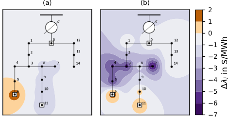
The case study is performed on the 15-node radial feeder from [9] with two minor modifications: one controllable DER is added at node 11 (see Fig. 3) and the power flow limit of edges 2 and 3 is doubled to avoid congestion in the deterministic case. Cost parameters of DERs at nodes 6 and 11 are set to $c_{1,i}=10\,\nicefrac{\mathrm{\$}}{\mathrm{MWh}}$ , $c_{2,i}=5\,\nicefrac{\mathrm{\$}}{\mathrm{MWh^{2}}}$ , $c_{0,i}=0$ . The substation cost is set to $c_{1,0}=50\,\nicefrac{\mathrm{\$}}{\mathrm{MWh}}$ , $c_{2,0}=400\,\nicefrac{\mathrm{\$}}{\mathrm{MWh^{2}}}$ , $c_{0,0}=0$ . Note that this selection incentivizes the use of DERs. The data of [9] is used as scheduled net demand with a normally distributed zero-mean error, standard deviation of $\sigma_{i}^{P}=0.2d_{i}^{P}$ and no covariance among the nodes. The security parameter of the chance constraints is set to $\epsilon_{g}=5\,\mathrm{\%}$ and $\epsilon_{v}=1\,\mathrm{\%}$ . All models in the case study are implemented using the Julia JuMP package and our code can be downloaded from [44].

Tables I, II and III summarize the optimal solution and prices in the deterministic, GEN-CC and VOLT-CC cases. Note that the deterministic case is solved for the expected net demand and $\alpha_{i}=0,\forall i$ . In the deterministic and GEN-CC cases, none of the generator limits are active and, therefore, their power production does not differ. Similarly the resulting voltage magnitudes do not change as the GEN-CC considers deterministic voltage constraints and only the flow limit of edges $8$ and $6$ are binding. In the VOLT-CC, however, the resulting voltage magnitudes are closer to unity in order to accommodate real-time power imbalances. As a result, the voltage constraints Equations 13d, 13e, 13f and 13g in the VOLT-CC yield non-zero dual multipliers. Figure 3 itemizes the effect of uncertainty on $\lambda^{P}_{i}$ relative to the deterministic case, where $\Delta\lambda^{P}_{i}=\lambda_{i}^{P,(\text{GEN-CC/VOLT-CC})}-\lambda_{i}^{P,(\text{DET})}$ . While the passive branch of the system (nodes $12$ to $14$ without any controllable DERs) shows no changes in DLMPs as it is fully supplied by the substation, DLMPs vary in the branches with DERs.

TABLE I: Optimal Deterministic Solution

$i$	$g_{i}^{P}$	$g_{i}^{Q}$	$\alpha_{i}$	$\sqrt{(f_{i}^{P})^{2}+(f_{i}^{Q})^{2}}$	$v_{i}$	$\lambda^{P}_{i}$
0	0.994	0.344	–	0.000	1.000	50.000
1	–	–	–	0.404	0.975	50.000
2	–	–	–	0.446	1.012	50.000
3	–	–	–	0.446	1.067	50.000
4	–	–	–	0.210	1.071	50.000
5	–	–	–	0.227	1.074	50.000
6	0.278	0.006	–	0.256^*	1.086	10.411
7	–	–	–	0.197	1.086	10.208
8	–	–	–	0.256^*	1.077	10.208
9	–	–	–	0.083	1.078	10.208
10	–	–	–	0.108	1.081	10.208
11	0.140	0.032	–	0.130	1.082	10.208
12	–	–	–	0.660	0.983	50.000
13	–	–	–	0.025	0.978	50.000
14	–	–	–	0.024	0.975	50.000
	^* Constraint is binding

TABLE II: Optimal GEN-CC Solution

$i$	$g_{i}^{P}$	$g_{i}^{Q}$	$\alpha_{i}$	$\sqrt{(f_{i}^{P})^{2}+(f_{i}^{Q})^{2}}$	$v_{i}$	$\lambda^{P}_{i}$	$\gamma$
0	0.994	0.344	0.003	0.000	1.000	50.00	0.273
1	–	–	–	0.404	0.975	50.00	–
2	–	–	–	0.446	1.012	50.00	–
3	–	–	–	0.446	1.067	50.00	–
4	–	–	–	0.210	1.071	50.00	–
5	–	–	–	0.227	1.074	50.00	–
6	0.278	0.006	0.646	0.256^*	1.086	11.99	–
7	–	–	–	0.197	1.086	8.769	–
8	–	–	–	0.256^*	1.077	8.769	–
9	–	–	–	0.083	1.078	8.769	–
10	–	–	–	0.108	1.081	8.769	–
11	0.140^*	0.032	0.351	0.130	1.082	8.769	–
12	–	–	–	0.660	0.983	50.00	–
13	–	–	–	0.025	0.978	50.00	–
14	–	–	–	0.024	0.975	50.00	–
	^* Constraint is binding

TABLE III: Optimal VOLT-CC Solution

$i$	$g_{i}^{P}$	$g_{i}^{Q}$	$\alpha_{i}$	$\sqrt{(f_{i}^{P})^{2}+(f_{i}^{Q})^{2}}$	$v_{i}$	$\lambda^{P}_{i}$	$\gamma$
0	1.033	0.490	0.377	0.000	1.000	50.00	31.51
1	–	–	–	0.523	0.956	49.97	–
2	–	–	–	0.439	0.972	47.88	–
3	–	–	–	0.439	0.996	44.59	–
4	–	–	–	0.208	0.997	44.83	–
5	–	–	–	0.222	0.999^*	45.056	–
6	0.258	-0.068	0.370	0.256^*	1.005^*	12.03	–
7	–	–	–	0.197	1.011^*	3.884	–
8	–	–	–	0.256^*	1.001	8.577	–
9	–	–	–	0.090	1.001	9.111	–
10	–	–	–	0.100	1.001^*	10.39	–
11	0.121	-0.040	0.253	0.116	1.002^*	10.95	–
12	–	–	–	0.660	0.983	50.00	–
13	–	–	–	0.025	0.978	50.00	–
14	–	–	–	0.024	0.975	50.00	–
	^* Constraint is binding

Tables IV and V itemize the components of the energy price following Proposition 1. Additionally, Fig. 4 illustrates the nodes and edges with binding limits and, thus, non-zero Lagrangian multipliers. Since the GEN-CC has no active voltage constraints the energy price at each node is determined by $\lambda^{P}_{\mathcal{A}_{i}}$ , i.e. the energy price at the ancestor node, and the congestion as per Equation 26. There is no reactive power price component due to inactive voltage limits. In the VOLT-CC case, on the other hand, the voltage limits become active and therefore reactive power price is non-zero.

In Fig. 3 we observe higher prices at and close to the nodes with DERs. As follows from Eq. Equation 29 and summarized in Table VI, prices at those nodes are dominated by the lower voltage limits, thus quantifying the value of downward regulation. A negative net demand value at node $7$ indicates a high uncontrolled behind-the-meter generation, which leads to low prices dominated by the upper voltage limit. This incentivizes a higher demand and lower generation. At node $6$ both the upper and lower voltage limits are binding (see Fig. 4 and non-zero $\mu_{6}^{+},\mu_{6}^{-}$ in the bottom row of Table VI), thus indicating that no more balancing regulation at this node is possible without increasing the likelihood of voltage limit violations. Hence, the trade-off between the power output and balancing regulation of the DER at node $6$ is no longer driven by its profit-maximizing objective, but rather by the the physical limits of the system.

Fig. 4: Illustration of binding edge, voltage and generation limits in the GEN-CC and the VOLT-CC.

TABLE IV: DLMP Decomposition of the GEN-CC, cf. Eq. (26)

$i$	$\lambda^{P}_{i}$	$\lambda^{P}_{\mathcal{A}_{i}}$	$\lambda^{Q}_{i}\frac{r_{i}}{x_{i}}$	$\lambda^{Q}_{\mathcal{A}_{i}}\frac{r_{i}}{x_{i}}$	$2\eta_{i}(f_{i}^{P}\!+\!\frac{r_{i}}{x_{i}}f_{i}^{Q})$
0	50.000	-0.000	-0.000	-0.000	0.000
1	50.000	50.000	0.000	0.000	-0.000
2	50.000	50.000	0.000	0.000	0.000
3	50.000	50.000	0.000	0.000	0.000
4	50.000	50.000	0.000	0.000	-0.000
5	50.000	50.000	0.000	0.000	0.000
6	11.996	50.000	0.000	0.000	38.004
7	8.769	8.769	0.000	0.000	0.000
8	8.769	50.000	0.000	0.000	41.231
9	8.769	8.769	0.000	0.000	-0.000
10	8.769	8.769	0.000	0.000	0.000
11	8.769	8.769	0.000	0.000	-0.000
12	50.000	50.000	0.000	0.000	0.000
13	50.000	50.000	0.000	0.000	0.000
14	50.000	50.000	0.000	0.000	0.000

TABLE V: DLMP Decomposition of the VOLT-CC, cf. Eq. (26)

$i$	$\lambda^{P}_{i}$	$\lambda^{P}_{\mathcal{A}_{i}}$	$\lambda^{Q}_{i}\frac{r_{i}}{x_{i}}$	$\lambda^{Q}_{\mathcal{A}_{i}}\frac{r_{i}}{x_{i}}$	$2\eta_{i}(f_{i}^{P}\!+\!\frac{r_{i}}{x_{i}}f_{i}^{Q})$
0	50.000	-0.000	-0.000	-0.000	0.000
1	49.976	50.000	0.024	0.000	-0.000
2	47.881	49.976	4.088	1.993	0.000
3	44.596	47.881	7.373	4.088	0.000
4	44.836	44.596	7.132	7.373	-0.000
5	45.056	44.836	6.887	7.108	0.000
6	12.025	45.056	0.000	6.911	39.942
7	3.884	8.577	7.072	2.379	0.000
8	8.577	44.596	2.376	7.369	41.012
9	9.111	8.577	1.842	2.376	-0.000
10	10.399	9.111	0.552	1.840	0.000
11	10.949	10.399	0.000	0.550	-0.000
12	50.000	50.000	0.000	0.000	0.000
13	50.000	50.000	0.000	0.000	0.000
14	50.000	50.000	0.000	0.000	0.000

TABLE VI: DLMP Decomposition of the VOLT-CC based on voltage constraints, cf. Eq. (29)

$i$	$\lambda^{P}_{i}$	$(\mu_{i}^{+}\!-\!\mu_{i}^{-})$	$\lambda^{P}_{\mathcal{A}_{i}}$	$2r_{i}\sum_{j\in\mathcal{D}_{i}}(\mu_{j}^{+}\!-\!\mu_{j}^{-})$	$2f_{i}^{P}\eta_{i}$
0	50.000	0.000	-0.000	-0.000	0.000
1	49.976	-0.000	50.000	0.024	-0.000
2	47.881	-0.000	49.976	2.096	0.000
3	44.596	-0.000	47.881	3.285	0.000
4	44.836	-0.000	44.596	-0.240	-0.000
5	45.056	-0.001	44.836	-0.220	0.000
6	12.025	-6.290^†	45.056	-0.606	33.638
7	3.884	44.871	8.577	4.694	0.000
8	8.577	-0.000	44.596	1.478	34.541
9	9.111	-0.000	8.577	-0.534	-0.000
10	10.399	-0.004	9.111	-1.288	0.000
11	10.949	-26.709	10.399	-0.550	-0.000
12	50.000	-0.000	50.000	-0.000	0.000
13	50.000	-0.000	50.000	-0.000	0.000
14	50.000	-0.000	50.000	-0.000	0.000
	^† $\mu_{6}^{+}=20.186$ , $\mu_{6}^{-}=26.476$

The regulation price in the GEN-CC case ( $\gamma^{\text{GEN-CC}}=0.273$ ) is notably lower relative to the VOLT-CC case ( $\gamma^{\text{VOLT-CC}}=31.511$ ). As per Proposition 2, $\gamma^{\text{GEN-CC}}$ is only driven by the power output limits (Table VII), where only the lower output limit at node $11$ is binding. Due to a low power price at node $11$ as compared to node $6$ , the scheduled power production is also low, which limits the downward regulation capacity provided. By introducing voltage chance constraints in the VOLT-CC case, the DLMP composition changes as per Proposition 3 (Table VII). Each node with binding voltage constraints ( $5,6,7,10,11$ ) contributes to the formation of $\gamma$ by weighting the impact of the system-wide regulation participation on the voltage standard deviation against the marginal value of relaxed voltage limits for each node (Eq. 45).

TABLE VII: Regulation Price Decomposition of the VOLT-CC

		GEN-CC		VOLT-CC
$i$	$b_{i}$	$\delta_{i}^{+}$	$\delta_{i}^{-}$	$\delta_{i}^{+}$	$\delta_{i}^{-}$	$\nu_{i}$
0	0.0005	–	–	–	–	–
1	–	–	–	–	–	0.120
2	–	–	–	–	–	10.699
3	–	–	–	–	–	27.281
4	–	–	–	–	–	28.199
5	–	–	–	–	–	29.040
6	0.1	-0.000	-0.000	-0.000	-0.000	31.357
7	–	–	–	–	–	32.533
8	–	–	–	–	–	30.201
9	–	–	–	–	–	30.472
10	–	–	–	–	–	31.126
11	0.1	-0.000	0.310	-0.000	-0.000	31.406
12	–	–	–	–	–	0.000
13	–	–	–	–	–	0.000
14	–	–	–	–	–	0.000

TABLE VIII: Optimal LVOLT-CC Solution

$i$	$g_{i}^{P}$	$g_{i}^{Q}$	$\alpha_{i}$	$\sqrt{(f_{i}^{P})^{2}+(f_{i}^{Q})^{2}}$	$v_{i}$	$\lambda^{P}_{i}$	$\gamma$
0	1.075	0.607	0.144	0.000	1.000	50.000	30.254
1	–	–	–	0.576	0.952	49.971	–
2	–	–	–	0.422	0.966	47.417	–
3	–	–	–	0.433	0.997	43.414	–
4	–	–	–	0.209	0.998	43.666	–
5	–	–	–	0.223	0.999	43.897	–
6	0.256	-0.077	0.515	0.256^*	1.005^*	14.005	–
7	–	–	–	0.197	1.016^*	6.372	–
8	–	–	–	0.256^*	1.006	4.169	–
9	–	–	–	0.079	1.007	4.169	–
10	–	–	–	0.102	1.009	4.169	–
11	0.137	0.012	0.341	0.124	1.011	4.169	–
12	–	–	–	0.661	0.983	50.000	–
13	–	–	–	0.026	0.978	50.000	–
14	–	–	–	0.024	0.975	50.000	–
	^* Constraint is binding

Table VIII summarizes the optimal LVOLT-CC solution obtained by using loss factor matrices $\LP^{P}$ , $\LP^{Q}$ , $\LQ^{P}$ , $\LQ^{Q}$ as defined in Equations 17 and 18 and shown in Fig. 5. Negative elements of the matrices shown in Fig. 5 indicate that additional DER production at node $j$ will increase power losses allocated to node $i$ based on FND. For example, $\LP^{P}$ shows that additional active production at nodes $0$ to $11$ will increase active power losses. On the other hand, additional active production on the passive branch (nodes $12$ to $14$ ), where no DERs are installed, will reduce active power losses.

Since increasing DER production at nodes $6$ and $11$ increases system losses, see Fig. 5, we observe that the power output of controllable DERs changes slightly, as compared to the results of the VOLT-CC, and the additional power needed to compensate for system losses is provided by the substation (node $0$ ). By internalizing the loss factors into the voltage chance constraints via matrix $R^{L}$ as in Equation 24, the impact of balancing participation on the voltage limits is no longer symmetric as in Equation 8. Thus, we observe higher balancing participation factors of the DERs at nodes $6$ and $11$ relative to the VOLT-CC. Additionally, a greater power supply from the substation and the DER at node $11$ leads to non-binding voltage constraints and, thus, uniform DLMPs at nodes $8$ to $11$ . In line with the theoretical results of Proposition 4a), the additional power losses have almost no impact on the price for balancing regulation. The small difference relative to the VOLT-CC is mainly caused by non-binding voltage constraints at nodes $10$ and $11$ .

This paper described an approach to derive stochasticity-aware DLMPs for electricity pricing in low-voltage electric power distribution systems that explicitly internalize uncertainty and risk parameters. These DLMPs are also shown to constitute a robust competitive equilibrium, which can be leveraged towards emerging distribution electricity market designs. In the future, our work will focus on the application of the proposed pricing theory to decentralized and communication-constrained control of DERs and for enabling electricity pricing in distribution systems with a high penetration rate of DERs and near-zero marginal production costs. Methodological extensions can encompass uncertainty internalization via semidefinite programming to allow for non-linear power flow representations, [45], and the impact of asymmetric information and strategic behavior.

[1] F. C. Schweppe et al., Spot pricing of electricity. Springer Science & Business Media, 2013.
[2] R. A. Verzijlbergh, L. J. De Vries, and Z. Lukszo, “Renewable energy sources and responsive demand. do we need congestion management?” IEEE Trans. Pwr. Sys., vol. 29, no. 5, pp. 2119–2128, 2014.
[3] P. M. Sotkiewicz and J. M. Vignolo, “Nodal pricing for distribution networks: efficient pricing for efficiency enhancing dg,” IEEE Trans. Pwr. Sys., vol. 21, no. 2, pp. 1013–1014, 2006.
[4] G. Heydt et al., “Pricing and control in the next power distribution system,” IEEE Trans. Sm. Gr., vol. 3, no. 2, pp. 907–914, 2012.
[5] L. Bai et al., “Distribution locational marginal pricing (dlmp) for congestion management and voltage support,” IEEE Trans. Pwr. Sys., vol. 33, no. 4, pp. 4061–4073, 2018.
[6] R. Li, Q. Wu, and S. S. Oren, “Distribution locational marginal pricing for optimal electric vehicle charging management,” IEEE Trans. Pwr. Sys., vol. 29, no. 1, pp. 203–211, 2014.
[7] S. Huang et al., “Distribution locational marginal pricing through quadratic programming for congestion management in distribution networks,” IEEE Trans. Pwr. Sys., vol. 30, no. 4, pp. 2170–2178, 2015.
[8] J. Zhao et al., “Congestion management method of low-voltage active distribution networks based on dlmp,” IEEE Access, 2019.
[9] A. Papavasiliou, “Analysis of distribution locational marginal prices,” IEEE Trans. Sm. Gr., vol. 9, no. 5, pp. 4872–4882, 2018.
[10] Z. Yuan, M. R. Hesamzadeh, and D. R. Biggar, “Distribution locational marginal pricing by convexified acopf and hierarchical dispatch,” IEEE Trans. Sm. Gr., vol. 9, no. 4, pp. 3133–3142, 2018.
[11] Y. Ding et al., “Real-time market concept architecture for ecogrid eu,” IEEE Trans. Sm. Gr., vol. 4, no. 4, pp. 2006–2016, 2013.
[12] M. Caramanis et al., “Co-optimization of power and reserves in dynamic t&d power markets with distributed energy resources,” Proceedings of the IEEE, vol. 104, no. 4, pp. 807–836, 2016.
[13] S. Wong and J. D. Fuller, “Pricing energy and reserves using stochastic optimization in an alternative electricity market,” IEEE Trans. Pwr. Sys., vol. 22, no. 2, pp. 631–638, 2007.
[14] J. M. Morales et al., “Pricing electricity in pools with wind producers,” IEEE Trans. Pwr. Sys., vol. 27, no. 3, pp. 1366–1376, 2012.
[15] S. Martín, Y. Smeers, and J. A. Aguado, “A stochastic two settlement equilibrium model for electricity markets with wind generation,” IEEE Trans. Pwr. Sys., vol. 30, no. 1, pp. 233–245, 2015.
[16] J. Kazempour, P. Pinson, and B. F. Hobbs, “A stochastic market design with revenue adequacy and cost recovery by scenario: Benefits and costs,” IEEE Trans. Pwr. Sys., vol. 33, no. 4, pp. 3531–3545, 2018.
[17] E. Dall’Anese, K. Baker, and T. Summers, “Chance-constrained ac optimal power flow for distribution systems with renewables,” IEEE Trans. Pwr. Sys., vol. 32, no. 5, pp. 3427–3438, 2017.
[18] D. Bienstock, M. Chertkov, and S. Harnett, “Chance-constrained optimal power flow: Risk-aware network control under uncertainty,” Siam Review, vol. 56, no. 3, pp. 461–495, 2014.
[19] Y. Dvorkin, M. Lubin, and L. Roald, “Chance constraints for improving the security of ac optimal power flow,” IEEE Trans. Power Syst., 2019.
[20] R. Mieth and Y. Dvorkin, “Online learning for network constrained demand response pricing in distribution systems,” arXiv preprint: 1811.09384, 2018.
[21] D. Ralph and Y. Smeers, “Risk trading and endogenous probabilities in investment equilibria,” SIAM Journal on Optimization, vol. 25, no. 4, pp. 2589–2611, 2015.
[22] A. Philpott, M. Ferris, and R. Wets, “Equilibrium, uncertainty and risk in hydro-thermal electricity systems,” Mathematical Programming, vol. 157, no. 2, pp. 483–513, Jun 2016. [Online]. Available: https://doi.org/10.1007/s10107-015-0972-4
[23] H. Ye et al., “Uncertainty marginal price, transmission reserve, and day-ahead market clearing with robust unit commitment,” IEEE Trans. Pwr. Sys., vol. 32, no. 3, pp. 1782–1795, 2017.
[24] X. Kuang et al., “Pricing chance constraints in electricity markets,” IEEE Trans. Pwr. Sys., vol. 33, no. 4, pp. 4634–4636, 2018.
[25] R. Mieth and Y. Dvorkin, “Data-driven distributionally robust power flow for distribution systems,” IEEE Ctr. Syst. Let., vol. 2, no. 3, 2018.
[26] A. Hassan et al., “Optimal load ensemble control in chance-constrained optimal power flow,” IEEE Trans. Sm. Gr., 2018.
[27] K. Baker and A. Bernstein, “Joint chance constraints in ac optimal power flow: Improving bounds through learning,” IEEE Trans. Sm. Gr., 2019.
[28] K. Bruninx et al., “Valuing demand response controllability via chance constrained programming,” IEEE IEEE Trans. Sustain. Energy, vol. 9, no. 1, pp. 178–187, 2017.
[29] Y. Dvorkin, “A chance-constrained stochastic electricity market,” arXiv preprint arXiv:1906.06963, 2019.
[30] R. Mieth, J. Kim, and Y. Dvorkin, “Risk-and variance-aware electricity pricing,” arXiv preprint arXiv:1910.05409, 2019.
[31] Y. Dvorkin et al., “Uncertainty sets for wind power generation,” IEEE Transactions on Power Systems, vol. 31, no. 4, pp. 3326–3327, 2015.
[32] L. Roald et al., “Security constrained optimal power flow with distributionally robust chance constraints,” arXiv preprint: 1508.06061, 2015.
[33] M. Lubin, Y. Dvorkin, and S. Backhaus, “A robust approach to chance constrained optimal power flow with renewable generation,” IEEE Trans. Pwr. Sys., vol. 31, no. 5, pp. 3840–3849, 2016.
[34] H. Wu et al., “Chance-constrained day-ahead scheduling in stochastic power system operation,” IEEE Transactions on Power Systems, vol. 29, no. 4, pp. 1583–1591, 2014.
[35] Next Kraftwerke. Balancing markets. [Online]. Available: https://www.next-kraftwerke.be/en/knowledge-hub/balancing-markets/
[36] M. E. Baran and F. F. Wu, “Optimal capacitor placement on radial distribution systems,” IEEE Trans. Power Del., vol. 4, no. 1, pp. 725–734, 1989.
[37] K. Turitsyn et al., “Local control of reactive power by distributed photovoltaic generators,” in IEEE Conf. Sm. Gr. Com., 2010, pp. 79–84.
[38] S. Wang et al., “Distributed generation hosting capacity evaluation for distribution systems considering the robust optimal operation of oltc and svc,” IEEE Transs on Sust. En., vol. 7, no. 3, pp. 1111–1123, 2016.
[39] H. Yuan et al., “Novel linearized power flow and linearized opf models for active distribution networks with application in distribution lmp,” IEEE Trans. Sm. Gr., vol. 9, no. 1, pp. 438–448, 2018.
[40] M. Farivar and S. H. Low, “Branch flow model: Relaxations and convexification—part i,” IEEE Transactions on Power Systems, vol. 28, no. 3, pp. 2554–2564, 2013.
[41] L. Wood et al., “Recovery of utility fixed costs: Utility, consumer, environmental and economist perspectives,” Lawrence Berkeley National Lab.(LBNL), Berkeley, CA (United States), Tech. Rep., 2016.
[42] M. E. Initative, “Utility of the future,” 2016. [Online]. Available: http://energy.mit.edu/research/utility-future-study/
[43] M. Farsi, M. Filippini et al., “A benchmarking analysis of electricity distribution utilities in switzerland,” Centre for Energy Policy and Economics Working Paper, no. 43, 2005.
[44] Code supplement - DLMPs under Uncertainty. [Online]. Available: https://github.com/korpuskel91/DLMP_uncertainty_CodeSupplement
[45] Z. Wang, D. S. Kirschen, and B. Zhang, “Accurate semidefinite programming models for optimal power flow in distribution systems,” arXiv preprint arXiv:1711.07853, 2017.

\begin{split}&c_{i}(\bm{g}_{i}^{P})=\frac{(g_{i}^{P}+\alpha_{i}\bm{\Omega}+a_{i})^{2}}{2b_{i}}+c_{i}\\ &=\frac{(g_{i}^{P})^{2}+\alpha_{i}^{2}\bm{\Omega}^{2}+a_{i}^{2}+2(g_{i}^{P}\alpha_{i}\bm{\Omega}+g_{i}^{P}a_{i}+\alpha_{i}\bm{\Omega}a_{i})}{2b_{i}}+c_{i}.\end{split}

(A-A.1)

Recall that $\Eptn[\bm{\omega}]=0$ . Then $\Eptn[e^{\!\top}\bm{\omega}]=\Eptn[\bm{\Omega}]=0$ and we obtain:

\begin{split}\Eptn[c_{i}(\bm{g}_{i}^{P})]&=\frac{(g_{i}^{P}+a_{i})^{2}}{2b_{i}}+c_{i}+\Eptn\left[\frac{\alpha_{i}^{2}\bm{\Omega}^{2}}{2b_{i}}\right]\\ &=c_{i}(g_{i}^{P})+\frac{\alpha_{i}^{2}}{2b_{i}}\Eptn\left[\bm{\Omega}^{2}\right]\end{split}

(A-A.2)

As $\Var[\bm{\bm{\Omega}}]=\Eptn[\bm{\Omega}^{2}]-\Eptn[\bm{\Omega}]^{2}$ and $\Var[\bm{\Omega}]=\Var[e^{\!\top}\bm{\omega}]=e^{\!\top}\Sigma e=s^{2}$ we find the respective expression $\Eptn\left[\bm{\Omega}^{2}\right]$ .

$\displaystyle(g_{i}^{P}):$

$\displaystyle\frac{(g_{i}+a_{i})}{b_{i}}+\delta_{i}^{+}-\delta_{i}^{-}-\pi_{i}^{g}=0$

$\displaystyle(\alpha_{i}):$

$\displaystyle\frac{\alpha_{i}}{b_{i}}s^{2}+z_{\epsilon_{g}}s(\delta_{i}^{+}+\delta_{i}^{-})-\pi^{\alpha}=0$

$\displaystyle 0\leq\delta_{i}^{+}\bot g_{i}^{P}+z_{\epsilon_{g}}\alpha_{i}s-g_{i}^{P,\max}\geq 0$

$\displaystyle 0\leq\delta_{i}^{-}\bot-g_{i}^{P}+z_{\epsilon_{g}}\alpha_{i}s+g_{i}^{P,\min}\geq 0.$

Using the expression for the uncertain voltage Equation 7, we can obtain

$\displaystyle\bm{u}_{i}(\bm{\omega},\alpha)-\bar{u}_{i}$	$\displaystyle=2[R(\bm{\omega}-\alpha e^{\!\top}\bm{\omega}]_{i}$
	$\displaystyle=2[R\bm{\omega}]_{i}-[R\alpha]_{i}(e^{\!\top}\bm{\omega})$	(A-B.1)
	$\displaystyle=2(R_{i*}-\rho_{i}^{v}e^{\!\top})\bm{\omega}.$

Then Eq. Equation 10 follows from:

\displaystyle\Var[\bm{u}_{i}(\bm{\omega},\alpha)]=4\left\lVert(R_{i*}-\rho_{i}^{v}e^{\!\top})\Sigma^{1/2}\right\rVert_{2}^{2}.

(A-B.2)