3DViewGraph: Learning Global Features for 3D Shapes from A Graph of Unordered Views with Attention
Abstract
Learning global features by aggregating information over multiple views has been shown to be effective for 3D shape analysis. For view aggregation in deep learning models, pooling has been applied extensively. However, pooling leads to a loss of the content within views, and the spatial relationship among views, which limits the discriminability of learned features. We propose 3DViewGraph to resolve this issue, which learns 3D global features by more effectively aggregating unordered views with attention. Specifically, unordered views taken around a shape are regarded as view nodes on a view graph. 3DViewGraph first learns a novel latent semantic mapping to project low-level view features into meaningful latent semantic embeddings in a lower dimensional space, which is spanned by latent semantic patterns. Then, the content and spatial information of each pair of view nodes are encoded by a novel spatial pattern correlation, where the correlation is computed among latent semantic patterns. Finally, all spatial pattern correlations are integrated with attention weights learned by a novel attention mechanism. This further increases the discriminability of learned features by highlighting the unordered view nodes with distinctive characteristics and depressing the ones with appearance ambiguity. We show that 3DViewGraph outperforms state-of-the-art methods under three large-scale benchmarks.
1 Introduction
Global features of 3D shapes can be learned from raw 3D representations, such as meshes, voxels, and point clouds. As an alternative, a number of works in 3D shape analysis employed multiple views Su and others 2015; Han et al. 2019b as raw 3D representation, exploiting the advantage that multiple views can facilitate understanding of both manifold and non-manifold 3D shapes via computer vision techniques. Therefore, effectively and efficiently aggregating comprehensive information over multiple views, is critical for the discriminability of learned features, especially in deep learning models.
Pooling was designed as a procedure for information abstraction in deep learning models. In order to describe a 3D shape by considering features from multiple views, view aggregation is usually performed by max or mean pooling, where pooling only employs the max or mean value of each dimension across all view features Su and others 2015. Although pooling is able to eliminate the rotation effect of 3D shapes, both the content information within views and the spatial relationship among views cannot be fully preserved. As a consequence, this limits the discriminability of learned features. In this work, we address the challenge to learn 3D features in a deep learning model by more effectively aggregating the content information within individual views, and the spatial relationship among multiple unordered views.
To tackle this issue, we propose a novel deep learning model called 3D View Graph (3DViewGraph), which learns 3D global features from multiple unordered views. By taking multiple views around a 3D shape on a unit sphere, we represent the shape as a view graph formed by the views, where each view denotes a node, and the nodes are fully connected with each other by edges. 3DViewGraph learns highly discriminative global 3D shape features by simultaneously encoding both the content information within the view nodes, and the spatial relationship among the view nodes.
- i)
We propose a novel deep learning model called 3DViewGraph for 3D global feature learning by effectively aggregating multiple unordered views. It not only encodes the content information within all views, but also preserves the spatial relationship among the views.
- ii)
We propose an approach to learn a low-dimensional latent semantic embedding of the views by directly capturing the similarities between each view and a set of latent semantic patterns. As an advantage, 3DViewGraph avoids mining the latent semantic patterns across the whole training set explicitly.
- iii)
We perform view aggregation by integrating a novel spatial pattern correlation, which encodes the content information and the spatial relationship in each pair of views.
- iv)
We propose a novel attention mechanism to increase the discriminability of learned features by highlighting the unordered view nodes with distinctive characteristics and depressing the ones with appearance ambiguities.
2 Related work
Deep learning models have made a big progress on learning 3D shape features from different raw representations, such as meshes Han and others 2018, voxels Wu and others 2016, point clouds Qi and others 2017 and views Su and others 2015. Because of page limit, we focus on reviewing view-based deep learning models to highlight the novelty of our view aggregation.
View-based methods. View-based methods represent a 3D shape as a set of rendered views Kanezaki et al. 2018 or panorama views Sfikas and others 2017. Besides direct set-to-set comparison Bai and others 2017, pooling is the widely used way of aggregating multiple views in deep learning models Su and others 2015. In addition to global feature learning, pooling can also be used to learn local features Huang et al. 2017; Yu et al. 2018 for segmentation or correspondence by aggregating local patches.
Although pooling can aggregate views on the fly in the models, it can not encode all the content information within views and the spatial relationship among views. Thus, the strategies of concatenation Savva and others 2016, view pair weighting Johns et al. 2016, cluster specified pooling Wang and others 2017, RNN Han and others 2019, were employed to resolve this issue. However, these methods can not learn from unordered views or fully capture the spatial information among unordered views.
To resolve the aforementioned issues, 3DViewGraph aggregates unordered views more effectively by simultaneously encoding their content information and spatial relationship.
Graph-based methods. To handle the irregular structure of graphs, various methods have been proposed Hamilton and others 2017. Although we formulate the multiple views from a 3D shape as a view graph, existing methods proposed for graphs cannot be directly used for learning the 3D feature in our scenario. The reasons are two-fold. First, these methods mainly focus on how to locally learn meaningful representation for each node in a graph from its raw attributes rather than globally learning the feature of the whole graph. Second, these methods mainly learns how to process the nodes in a graph with firm order, while the order of views involved in 3DViewGraph are always ambiguous because of the rotation of 3D shapes.
Moreover, some methods have employed graphs to retrieve 3D shapes from multiple views Anan et al. 2015; An-An et al. 2016. Different from these methods, 3DViewGraph employs a more efficient way of view aggregation in deep learning models, which makes the learned features useful for both classification and retrieval.
3 3DViewGraph

Overview. Fig. 1 shows an overview of 3DViewGraph, where the global feature of a 3D shape is learned from its corresponding view graph . Here, is the -th shape in a training set of 3D shapes, where . Based on the -dimensional feature , 3DViewGraph classifies into one of shape classes according to the probability , which is provided by a final softmax classifier (Fig. 1(f)), where is the class label of .
We first take a set of unordered views on a unit sphere centered at , as shown in Fig. 1(a). Here, we use “unordered views” to indicate that the views cannot be organized in a sequential way. The views are regarded as view nodes (briefly shown by symbols) of an undirected graph , where each is fully connected with other view nodes by edges , such that .
Next, we extract low-level features of each view using a fine-tuned VGG19 network Simonyan and Zisserman 2014, as shown in Fig. 1(b), where is extracted from the last fully connected layer. To obtain lower-dimensional, semantically more meaningful view features, we subsequently learn a latent semantic mapping (Fig. 1(c)) to project a low-level view feature into its latent semantic embedding .
To resolve the effect of rotation, 3DViewGraph encodes the content and spatial information of by exhaustively computing our novel spatial pattern correlation between each pair of view nodes. As illustrated in Fig. 1(d), we compute the pattern correlation between and each other node , and we weight it with their spatial similarity . In addition, for each node , we compute its cumulative correlation to summarize all spatial pattern correlations as the characteristics of the 3D shape from the -th view node .
Finally, we obtain the global feature of shape by integrating all cumulative correlations with our novel attention weights , as shown in Fig. 1(e) and (f). aims to highlight the view nodes with distinctive characteristics while depressing the ones with appearance ambiguity.
Latent semantic mapping learning. To learn global features from unordered views, 3DViewGraph encodes the content information within all views and the spatial relationship among views in a pairwise way. 3DViewGraph relies on the intuition that correlations between pairs of views can effectively represent discriminative characteristics of a 3D shape, especially considering the relative spatial position of the views. To implement this intuition, each view should be encoded in terms of a small set of common elements across all views in the training set. Unfortunately, the low-level features are too high dimensional and not suitable as a representation of the views in terms of a set of common elements.

To resolve this issue, 3DViewGraph introduces a latent semantic mapping by learning a kernel function to directly capture the similarities between views and latent semantic patterns . Our approach avoids additionally and explicitly mining across the whole training set as the common elements. projects low-level view features into latent semantic space spanned by as latent semantic emdeddings . represents view nodes with more semantic meaning but lower dimension than . Specifically, predicted by kernel , the -th dimension of characterizes the similarity between and the -th semantic pattern , such that . We define the kernel as
| (1) |
where the similarity is inversely proportional to the distance between and through , and gets normalized across the similarities between and all . Parameter controls the decay of the response with the distance. This equation can be further simplified by cancelling the norm of from the numerator and the denominator as follows,
| (2) |
where in the last step, we substituted and by and , respectively. Here, , and are sets of learnable parameters, in addition, both and depend on . However, to obtain more flexible training by following the viewpoint in Arandjelovic and others 2016, we employ two independent sets of , , decoupling and from . This decoupling enables 3DViewGraph to directly predict the similarity between and by the kernel without explicitly mining across all low-level view features in the training set.
Based on the last line in Eq. 2, we implement the latent semantic mapping as a row-wise convolution with each pair of and corresponding to a filter and a row-wise softmax normalization, as shown in Fig. 2.
Spatial pattern correlation. The pattern correlation aims to encode the content of view nodes and . makes the semantic patterns that co-occur in both views more prominent while the non-co-occurring ones more subtle. More precisely, we use the latent semantic embeddings and to compute as follows,
| (3) |
where is a dimensional matrix whose entry measures the correlation between the semantic pattern contributing to and contributing to .

We further enhance the pattern correlation between the view nodes and by their spatial similarity , which forms the spatial pattern correlation .
Fig. 3 visualizes how we compute the spatial similarity . In Fig. 3(a), we show all edges connecting to all other view nodes in different colors, where is briefly shown by symbols. The length of is measured by the length of the shortest arc connecting the two view nodes and on the unit sphere. Thus, as illustrated in Fig. 3(b), where is the central angle of the arc and the factor corresponds to the radius of the unit sphere. To reduce the high variance of , we employ instead of , which normalizes into the range of . Finally, is inversely proportional to as follows,
| (4) |
where is a parameter to control the decay of the response with the edge length. In Fig. 3(c), we visualize by mapping the value of to the width of edges .
To represent the characteristics of 3D shape from the -th view node on , we finally introduce the cumulative correlation , which encodes all spatial pattern correlations starting from as follows,
| (5) |
Attentioned correlation aggregation. Intuitively, more views will provide more information to any deep learning model, which should allow it to produce more discriminative 3D features. However, additional views may also introduce appearance ambiguities that negatively affect the discriminability of learned features, as shown in Fig. 4.

To resolve this issue, 3DViewGraph employs a novel attention mechanism in the aggregation of the 3D shape characteristics from all unordered view nodes of a shape, as illustrated in Fig. 1(e). 3DViewGraph learns attention weights for all view nodes on , where would be a large value (the second row in Fig. 4) if the view has distinctive characteristics, while would be a small value (the first row in Fig. 4) if exhibits appearance ambiguity with views from other shapes. Note that .
Our novel attention mechanism evaluates how distinctive each view is to the views that 3DViewGraph has processed. To comprehensively represent the characteristics of the views that 3DViewGraph has processed, the attention mechanism employs the fully connected weights in the final softmax classifier which accumulates the information of all views, as shown in Fig. 1(f). The attention mechanism projects the characteristics of 3D shape from the -th view node and the characteristics of the views that 3DViewGraph has processed into a common space to calculate the distinctiveness of view , as defined below,
| (6) | ||||
where , , , and are learnable parameters in the attention mechanism, , where is the dimension of the learned global feature , and is the number of shape classes. With and , is projected into a dimensional space, where is a bias in that space. In addition, is projected into the same space by to compute the similarities between and along all dimensions. Subsequently, the attention weight is calculated by comprehensively summarizing all similarities along all the dimensions with a linear mapping . Finally, the in for all views of -th shape are normalized by softmax normalization.
Based on , the characteristics of 3D shape from all view nodes are aggregated with weighting into attentioned correlation aggregation , as defined below,
| (7) |
where represents 3D shape as a matrix, as shown in Fig. 1(e). Finally, the global feature of 3D shape is learned by a fully connected layer with attentioned correlation aggregation as input, as shown in Fig. 1(f), where the fully connected layer is followed by a sigmoid function.
Using , the final softmax classifier computes the probabilities to classify the 3D shape into one of shape classes as
| (8) |
where and are learnable parameters for the computation of . is used to represent all the characteristics of views that 3DViewGraph has processed, as employed to calculate in Eq. 6.
Learning inference. The parameters involved in 3DViewGraph are optimized by minimizing the log-likelihood over 3D shapes in the training set, where is the truth label,
| (9) |
The parameter optimization is conducted by back propagation of classification errors of 3D shapes. Noteworthy, is updated by two elements with the learning rate as follows,
| (10) |
The advantage of Eq. (10) is that can be learned more flexibly for optimization convergence. also enables to simultaneously observe the characteristics of shape from each view node and take all views that have been processed from different shapes as reference.
4 Results and analysis
We evaluate 3DViewGraph by comparing it with the state-of-the-art methods in shape classification and retrieval under ModelNet40 Wu and others 2015, ModelNet10 and ShapeNetCore55 Savva and others 2017. We also show ablation studies to justify the effectiveness of novel elements.
| 64 | 128 | 256 | 512 | 1024 | |
|---|---|---|---|---|---|
| Acc % | 93.44 | 93.03 | 93.80 | 93.07 | 93.19 |
Parameters. We first explore how the important parameters , and affect the performance of 3DViewGraph under ModelNet40. The comparison in Table. 1, 2, and 3 shows that their effects are slight in a proper range.
| 32 | 64 | 128 | 256 | 512 | |
|---|---|---|---|---|---|
| Acc % | 90.84 | 92.91 | 93.80 | 93.44 | 93.40 |
Classification. As compared under ModelNet in Table 4, 3DViewGraph outperforms all the other methods under the same condition11 1 We use the same modality of views from the same camera system for the comparison, where the results of RotationNet are from Fig.4 (d) and (e) in https://arxiv.org/pdf/1603.06208.pdf. Moreover, the benchmarks are with the standard training and test split.. In addition, we show the single view classification accuracy in VGG fine-tuning (“VGG(ModelNet)”). To highlight the contribution of VGG fine-tuning, spatial similarity, and attention, we remove fine-tuning (“Ours(No finetune)”) or set all spatial similarity (“Ours(No spatiality)”) and attention (“Ours(No attention)”) to 1. The degenerated results indicate these elements are important for 3DViewGraph to achieve high accuracy. Similar phenomena is observed when we justify the effect of and in Eq. 6 by setting them to 1 (“Ours(No attention-)”), respectively. We also justify the latent semantic embedding and spatial pattern correlation by replacing them by single view features (“Ours(No latent)”) and summation (“Ours(No correlation)”), the degenerated results also show that they are important elements. Finally, we compare our proposed view aggregation with mean (“Ours(MeanPool)”) and max pooling (“Ours(MaxPool)”) by directly pooling all single view features together. Due to the loss of content information in each view and spatial information among multiple views, pooling performs worse.
| 0 | 1 | 5 | 10 | 11 | |
|---|---|---|---|---|---|
| Acc % | 92.91 | 93.48 | 93.72 | 93.80 | 93.48 |
| Methods | MN40(%) | MN10(%) |
|---|---|---|
| 3DGANWu and others 2016 | 83.3 | 91.0 |
| PointNet++Qi and others 2017 | 91.9 | - |
| FoldingNetYang et al. 2018 | 88.4 | 94.4 |
| PANOSfikas and others 2017 | 90.7 | 91.1 |
| PairwiseJohns et al. 2016 | 90.7 | 92.8 |
| GIFTBai and others 2017 | 89.5 | 91.5 |
| DomiWang and others 2017 | 92.2 | - |
| MVCNNSu and others 2015 | 90.1 | - |
| SphericalCao et al. 2017 | 93.31 | - |
| RotationKanezaki et al. 2018 | 92.37 | 94.39 |
| SO-NetLi and others 2018 | 90.9 | 94.1 |
| SVSLHan and others 2019 | 93.31 | 94.82 |
| VIPGANHan et al. 2019a | 91.98 | 94.05 |
| VGG(ModelNet40) | 87.27 | - |
| VGG(ModelNet10) | - | 88.63 |
| Ours | 93.80 | 94.82 |
| Ours() | 93.72 | 95.04 |
| Ours(No finetune) | 90.40 | - |
| Ours(No spatiality) | 92.91 | 94.16 |
| Ours(No attention) | 93.07 | 93.72 |
| Ours(No attention-) | 91.82 | 93.39 |
| Ours(No attention-) | 91.57 | 93.28 |
| Ours(No latent) | 92.34 | 92.95 |
| Ours(No correlation) | 89.30 | 93.83 |
| Ours(MeanPool) | 92.38 | 93.06 |
| Ours(MaxPool) | 91.89 | 92.84 |
3DViewGraph also achieves the best under the more challenging benchmark ShapeNetCore55, based on the fine-tuned VGG (“VGG(ShapeNetCore55)”), as shown in Table 5. We also find that different parameters do not significantly affect the performance, such as and .
| Methods | Views | Accuracy(%) |
|---|---|---|
| VIPGANHan et al. 2019a | 12 | 82.97 |
| SVSLHan and others 2019 | 12 | 85.47 |
| VGG(ShapeNetCore55) | 1 | 81.33 |
| Ours | 20 | 86.87 |
| Ours() | 20 | 86.36 |
| Ours() | 20 | 86.56 |
| Ours(,) | 20 | 86.71 |

Attention visualization. We visualize the attention learned by 3DViewGraph under ModelNet40, which demonstrates how 3DViewGraph understands 3D shapes by analyzing views on a view graph. In Fig. 5, attention weights on view nodes of are visualized as a vector which is represented by scattered black nodes, where the corresponding views are also shown nearby, such as the views of a toilet in Fig. 5(a), a table in Fig. 5(b) and a cone in Fig. 5(c). The coordinates of black nodes along the y-axis indicate how much attention 3DViewGraph pays to the corresponding view nodes. In addition, the views that is paid the most and least attention to are highlighted by the red upward and blue downward arrow, respectively.
| micro | macro | |||||||||
|---|---|---|---|---|---|---|---|---|---|---|
| Methods | P@N | R@N | F1@N | mAP@N | NDCG@N | P@N | R@N | F1@N | mAP@N | NDCG@N |
| All | 0.818 | 0.803 | 0.798 | 0.772 | 0.865 | 0.618 | 0.667 | 0.590 | 0.583 | 0.657 |
| Taco | 0.701 | 0.711 | 0.699 | 0.676 | 0.756 | - | - | - | - | - |
| Ours | 0.6090 | 0.8034 | 0.6164 | 0.8492 | 0.9054 | 0.1929 | 0.8301 | 0.2446 | 0.7019 | 0.8461 |
| Methods | Range | MN40 | MN10 |
| SHD | Test-Test | 33.26 | 44.05 |
| LFD | Test-Test | 40.91 | 49.82 |
| 3DNetsWu and others 2015 | Test-Test | 49.23 | 68.26 |
| GImageSinha et al. 2016 | Test-Test | 51.30 | 74.90 |
| DPanoShi and others 2015 | Test-Test | 76.81 | 84.18 |
| MVCNNSu and others 2015 | Test-Test | 79.50 | - |
| PANOSfikas and others 2017 | Test-Test | 83.45 | 87.39 |
| GIFTBai and others 2017 | Random | 81.94 | 91.12 |
| TripletHe et al. 2018 | Test-Test | 88.0 | - |
| Ours | Test-Test | 90.54 | 92.40 |
| Ours | Test-Train | 93.49 | 95.17 |
| Ours | Train-Train | 98.75 | 99.79 |
| Ours | All-All | 96.95 | 98.52 |

Fig. 5 demonstrates that 3DViewGraph is able to understand each view, since the view with the most ambiguous appearance in a view graph is depressed while the view with the most distinctive appearance is highlighted. For example, the most ambiguous views of toilet, table and cone merely show some basic shapes that provide little useful information for classification, such as the rectangles of the toilet and table, and the circle of the cone. In contrast, the most distinctive views of toilet, table and cone exhibit more unique and distinctive characteristics.
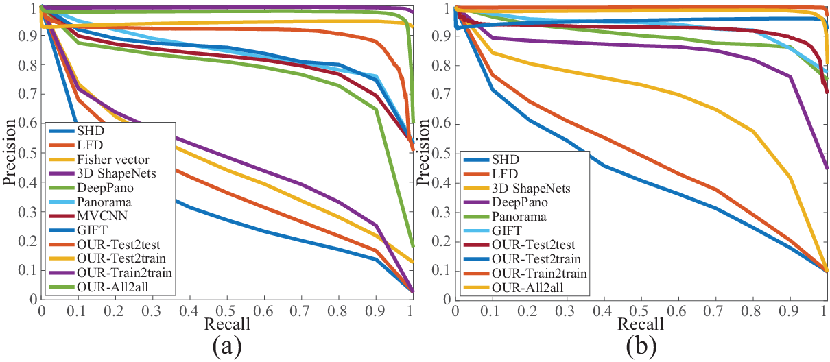
Retrieval. We evaluate the retrieval performance of 3DViewGraph under ModelNet in Table 7. We outperform the state-of-the-art methods, where the retrieval range is also shown. We further detail the precision and recall curves of these results in Fig. 7. In addition, 3DViewGraph also achieve the best results under ShapeNetCore55 in Table 6. We compare 10 state-of-the-art methods under testing set in the SHREC2017 retrieval contest Savva and others 2017 and Taco Cohen et al. 2018, where we summarize all the 10 methods (“All”) by presenting the best result of each metric due to page limit. Finally, we demonstrate that 3DViewGraph is also superior to other graph-based multi-view learning methods Anan et al. 2015; An-An et al. 2016 under Princeton Shape Benchmark (PSB) in Fig. 6.
5 Conclusion
In view-based deep learning models for 3D shape analysis, view aggregation via widely used pooling, leads to information loss about content and spatial relationship of views. We propose 3DViewGraph to address this issue for 3D global feature learning by more effectively aggregating unordered views with attention. By organizing unordered views taken around a 3D shape into a view graph, 3DViewGraph learns global features of the 3D shape by simultaneously encoding both the content information within view nodes and the spatial relationship among the view nodes. Through a novel latent semantic mapping, low-level view features are projected into a meaningful, lower-dimensional latent semantic embedding using a learned kernel function, which directly captures the similarities between low-level view features and latent semantic patterns. The latent semantic mapping successfully facilitates 3DViewGraph to encode the content information and the spatial relationship in each pair of view nodes using a novel spatial pattern correlation. Further, our novel attention mechanism effectively increases the discriminability of learned features by efficiently highlighting the unordered view nodes with distinctive characteristics and depressing the ones with appearance ambiguity. Our results in classification and retrieval under three large-scale benchmarks show that 3DViewGraph can learn better global features than the state-of-the-art methods due to its more effective view aggregation.
6 Acknowledgments
This work was supported by National Key R&D Program of China (2018YFB0505400), NSF (1813583), University of Macau (MYRG2018-00138-FST), and FDCT (273/2017/A). We thank all anonymous reviewers for their constructive comments.
References
- An-An et al. [2016] Liu An-An, Nie Wei-Zhi, and Su Yu-Ting. Multi-modal clique-graph matching for view-based 3D model retrieval. IEEE Transactions on Image Processing, 25(5):2103–2115, 2016.
- Anan et al. [2015] Liu Anan, Wang Zhongyang, Nie Weizhi, and Su Yuting. Graph-based characteristic view set extraction and matching for 3D model retrieval. Information Sciences, 320:429–442, 2015.
- Arandjelovic and others [2016] Relja Arandjelovic et al. NetVLAD: CNN architecture for weakly supervised place recognition. In IEEE Conference on Computer Vision and Pattern Recognition, pages 5297–5307, 2016.
- Bai and others [2017] Song Bai et al. GIFT: Towards scalable 3D shape retrieval. IEEE Transaction on Multimedia, 19(6):1257–1271, 2017.
- Cao et al. [2017] Zhangjie Cao, Qixing Huang, and Karthik Ramani. 3D object classification via spherical projections. In International Conference on 3D Vision. 2017.
- Cohen et al. [2018] Taco S. Cohen, Mario Geiger, Jonas Köhler, and Max Welling. Spherical CNNs. In International Conference on Learning Representations, 2018.
- Hamilton and others [2017] William L. Hamilton et al. Representation learning on graphs: Methods and applications. IEEE Data Engineering Bulletin, 40(3):52–74, 2017.
- Han and others [2018] Zhizhong Han et al. Deep spatiality: Unsupervised learning of spatially-enhanced global and local 3D features by deep neural network with coupled softmax. IEEE Transactions on Image Processing, 27(6):3049–3063, 2018.
- Han and others [2019] Zhizhong Han et al. Seqviews 2seqlabels: Learning 3D global features via aggregating sequential views by rnn with attention. IEEE Transactions on Image Processing, 28(2):1941–0042, 2019.
- Han et al. [2019a] Zhizhong Han, Mingyang Shang, Yu-Shen Liu, and Matthias Zwicker. View inter-prediction gan: Unsupervised representation learning for 3D shapes by learning global shape memories to support local view predictions. In AAAI, 2019.
- Han et al. [2019b] Zhizhong Han, Mingyang Shang, Xiyang Wang, Yu-Shen Liu, and Matthias Zwicker. Y2seq2seq: Cross-modal representation learning for 3D shape and text by joint reconstruction and prediction of view and word sequences. In AAAI, 2019.
- He et al. [2018] Xinwei He, Yang Zhou, Zhichao Zhou, Song Bai, and Xiang Bai. Triplet-center loss for multi-view 3D object retrieval. In The IEEE Conference on Computer Vision and Pattern Recognition, 2018.
- Huang et al. [2017] H. Huang, E. Kalegorakis, S. Chaudhuri, D. Ceylan, V. Kim, and E. Yumer. Learning local shape descriptors with view-based convolutional neural networks. ACM Transactions on Graphics, 2017.
- Johns et al. [2016] Edward Johns, Stefan Leutenegger, and Andrew J. Davison. Pairwise decomposition of image sequences for active multi-view recognition. In IEEE Conference on Computer Vision and Pattern Recognition, pages 3813–3822, 2016.
- Kanezaki et al. [2018] Asako Kanezaki, Yasuyuki Matsushita, and Yoshifumi Nishida. Rotationnet: Joint object categorization and pose estimation using multiviews from unsupervised viewpoints. In IEEE Conference on Computer Vision and Pattern Recognition, 2018.
- Li and others [2018] Jiaxin Li et al. SO-Net: Self organizing network for point cloud analysis. In The IEEE Conference on Computer Vision and Pattern Recognition, 2018.
- Qi and others [2017] Charles Qi et al. Pointnet++: Deep hierarchical feature learning on point sets in a metric space. In Advances in Neural Information Processing Systems, pages 5105–5114, 2017.
- Savva and others [2016] M. Savva et al. Shrec’16 track large-scale 3D shape retrieval from shapeNet core55. In EG 2016 workshop on 3D Object Recognition, 2016.
- Savva and others [2017] Manolis Savva et al. SHREC’17 Large-Scale 3D Shape Retrieval from ShapeNet Core55. In Eurographics Workshop on 3D Object Retrieval, 2017.
- Sfikas and others [2017] Konstantinos Sfikas et al. Exploiting the PANORAMA Representation for Convolutional Neural Network Classification and Retrieval. In EG Workshop on 3D Object Retrieval, pages 1–7, 2017.
- Shi and others [2015] B. Shi et al. Deeppano: Deep panoramic representation for 3D shape recognition. IEEE Signal Processing Letters, 22(12):2339–2343, 2015.
- Simonyan and Zisserman [2014] K. Simonyan and A. Zisserman. Very deep convolutional networks for large-scale image recognition. CoRR, abs/1409.1556, 2014.
- Sinha et al. [2016] Ayan Sinha, Jing Bai, and Karthik Ramani. Deep learning 3D shape surfaces using geometry images. In European Conference on Computer Vision, pages 223–240, 2016.
- Su and others [2015] Hang Su et al. Multi-view convolutional neural networks for 3D shape recognition. In International Conference on Computer Vision, pages 945–953, 2015.
- Wang and others [2017] Chu Wang et al. Dominant set clustering and pooling for multi-view 3D object recognition. In British Machine Vision Conference, 2017.
- Wu and others [2015] Zhirong Wu et al. 3D ShapeNets: A deep representation for volumetric shapes. In Proceedings of IEEE Conference on Computer Vision and Pattern Recognition, pages 1912–1920, 2015.
- Wu and others [2016] Jiajun Wu et al. Learning a probabilistic latent space of object shapes via 3D generative-adversarial modeling. In Advances in Neural Information Processing Systems, pages 82–90, 2016.
- Yang et al. [2018] Yaoqing Yang, Chen Feng, Yiru Shen, and Dong Tian. Foldingnet: Point cloud auto-encoder via deep grid deformation. In IEEE Conference on Computer Vision and Pattern Recognition, 2018.
- Yu et al. [2018] Tan Yu, Jingjing Meng, and Junsong Yuan. Multi-view harmonized bilinear network for 3D object recognition. In The IEEE Conference on Computer Vision and Pattern Recognition, 2018.