TASI Lectures on Future Colliders
Abstract:
These lectures review the main motivations for future high-energy colliders, focusing on the understanding of electroweak symmetry breaking and on the search for physics beyond the Standard Model. The open questions and the challenges are common to all future projects; for concreteness, I will use studies of the potential of and pp circular colliders to provide examples of the anticipated physics reach.
CERN-TH-2019-073
4 - 29 June, 2018
Boulder, Colorado
1 Introduction
Several projects for future high-energy particle colliders are under consideration in various regions worldwide, to complement and extend the physics reach of CERN’s Large Hadron Collider (LHC). These include:
- •
- •
- •
the Future Circular Collider (FCC [9, 10, 11, 12]) and the CEPC/SppC [13, 14], two similar projects promoted by CERN and China respectively, envisioning a staged facility, enabled by a 100 km circular ring, designed to deliver collisions at energies in the range GeV, pp collisions up to TeV, ep collisions at TeV, as well as heavy ion collisions.
This variety of layouts (circular or linear), beam types (electrons or protons) and energies, reflects slightly different priorities for the physics targets and observables, as well as a different judgement on the overall balance between physics returns, technological challenges and feasibility, time scales for completion and exploitation, and financial/political realities.
If approved today, the projects in this list could in principle begin delivering physics results at some point during the decade 2030-40, and operate for the following 15-25 years, depending on the technology and upgrade path. Beyond this, but with an unspecified time scale, ideas are on the table for a possible subsequent generation of even more ambitious lepton-collider projects, which I only mention here: linear electron accelerators based on multi-GeV/m gradient technologies like plasma wake fields or lasers [15], and muon circular colliders [16, 17].
The FCC and SppC proton colliders would face a preparatory phase longer than the colliders, mostly because of the R&D period required to produce reliable and affordable SC bending magnets with the 16 T magnetic field needed to keep 50 TeV protons in orbit in the 100 km ring (A 12 T option, based on high-Tc SCs, is considered for SppC, but is itself far from being established).
No matter what the energy or the technology, all these projects share common goals, driven by the need to clarify several outstanding open issues in particle physics. This need singles out the next generation of colliders beyond the LHC as unique and indispensable exploratory tools to continue driving the progress in our understanding of nature.
In these lectures, I will review the main motivations for future high-energy colliders and discuss their physics potential. I will mostly cover topics such as Higgs and physics beyond the Standard Model (BSM), and, while I will recall some basic theoretical background, I will give for granted that students know those topics from their studies, or from other lectures in the TASI program. In particular, in 2018 students have been exposed, among others, to excellent lectures on the Higgs boson [18]), supersymmetry and dark matter [19], QCD at colliders [20], effective field theory [21] and flavour [22]. I refer to these, and to the great lectures on LHC physics by our host Tilman Plehn [23], for the necessary background material.
I will illustrate the value of the physics reach through concrete examples of the FCC physics potential. No attempt is made here to compare the FCC against the other projects, as the point of these lectures is not to promote one project over another: I choose here the FCC since it is the project that I know better, and the one that, in terms of breadth, variety and physics performance, best illustrates how ambitious the targets of a future collider can be.
I will include also a few exercises here and there. They are meant to stimulate your thinking, they are simple, do not necessarily require calculations and are mostly for a qualitative discussion. But if you take them seriously, some of them could be the seed for interesting work!
2 Where we stand
In almost ten years of studies at the LHC, the picture of the particle physics landscape has greatly evolved. The legacy of this first phase of the LHC physics programme can be briefly summarised in three points: a) the discovery of the Higgs boson, and the start of a new phase of detailed studies of its properties, aimed at revealing the deep origin of electroweak (EW) symmetry breaking; b) the indication that signals of new physics around the TeV scale are, at best, elusive; c) the rapid advance of theoretical calculations, whose constant progress and reliability underline the key role of ever improving precision measurements, from the Higgs to the flavour sectors. Last but not least, the LHC success has been made possible by the extraordinary achievements of the accelerator and of the detectors, whose performance is exceeding all expectations, supporting the confidence in the ability of the next generation of colliders to achieve what they promise.
2.1 The puzzling origin of the Higgs field
The years that preceded the discovery of the Higgs boson have been characterized by a general strong belief in its existence, justified by the success of the Standard Model (SM), and by the confidence that EW symmetry breaking (EWSB) is indeed driven by the basic dynamics of the Higgs mechanism, as described in the SM. Starting from this assumption, the theoretical speculations focused on identifying possible solutions to the hierarchy problem, namely the extreme fine tuning required to achieve the decoupling of the Higgs and EW mass scale from the phenomena expected to emerge at much higher energy scales, up to the Planck scale. These speculations led to the consideration of several possible scenarios of new physics, from supersymmetry to large extra dimensions, which would provide natural solutions to the hierarchy problem by introducing new degrees of freedom, new symmetries, or new dynamics at the TeV scale. The opportunity to combine the solution of the hierarchy problem with the understanding of experimental facts such as the existence of dark matter, or of the features of flavour phenomena, gave further impetus to these theoretical efforts, and to the many experimental studies dedicated to the search for BSM manifestations.
The conceptual simplicity and appeal of several of these scenarios, justified optimism that their concrete manifestations would appear “behind the corner”. After all, the SM itself was born as the simplest possible model in which to embed an elegant explanation (the Higgs mechanism) to the problem of justifying the mass of the weak force carrier and parity non-conservation, and this simple framework DID work! Why shouldn’t the next step beyond the SM be accomplished by similarly elegant and “simple” proposals?
Lack of evidence of new physics at the TeV scale, made even more compelling by the hundreds of inconclusive searches scrupolously carried out by the LHC experiments, has not removed, however, the need to continue addressing the original motivations for a BSM extension of the SM. If anything, this has made the open issues even more intriguing, and challenging. But, while the efforts to review the underlying perspective on the hierarchy problem and naturalness continue, we should focus on a perhaps even more basic question: who ordered the Higgs? Where does the famous “mexican hat” Higgs potential come from? This appears like a pointless trivial question. A sort of mexican-hat potential must be there, it’s a necessary ingredient in the realization of EWSB, without it we would not be here discussing it. But what is its true origin?
To understand the value of this question, it is useful to compare the dynamics of the Higgs field with that of electromagnetism (EM), or of any of the other known fundamental forces in nature. All properties of EM arise from a simple principle, the gauge principle. Coulomb’s law has no free parameter, except the overall scale of the electric charge, absorbed in the definition of the charge unit. The quantization of the charge may have a deep origin in quantum mechanical properties such as anomaly cancellation, or in the algebraic structure of the representations of larger gauge groups in which EM is embedded. The sign of the electric force, positive or negative depending on the relative sign of the interacting charges, follows from the spin-1 nature of the photon. The behaviour follows from the Gauss theorem, or charge conservation, or gauge invariance, depending on how we want to phrase it. We do not know why nature has chosen gauge symmetry as a guiding principle, although this appears as an unavoidable consequence of the existence of interactions mediated by massless particles, which are the basis of the long-range forces needed to sustain our existence. But gauge symmetry appears everywhere, e.g. in the zero modes of a string theory, or as a result of compactification in Kaluza-Klein gravitational theories. Gauge symmetry is therefore intimately related to possible deeper properties of nature.
On the contrary, nothing is fundamental in the Higgs potential, there doesn’t seem to be any fundamental symmetry or underlying principle that controls its structure. To fix the notation for further use, we shall write this potential as
| (1) |
where is the SU(2) doublet scalar field and is the real part of the neutral component ( being its vacuum expectation value). The condition of minimum of the potential () and the Higgs mass definition () lead to the relations and , expressed in terms of the measured Higgs mass and of Fermi’s coupling GeV. The sign and value of the parameters and are a priori arbitrary. A negative sign in front of the quadratic term is required to achieve symmetry breaking, but is not required by any symmetry. The positive sign of is necessary for the stability of the potential at large but, again, is not dictated by anything: it could be negative, and the potential could be stabilized at larger values by higher-order terms. Even the functional form is not fundamental: the underlying gauge symmetry only requires the potential to depend on , and the quartic form could simply represent the leading terms in the power expansion of a more complex functional dependence of the potential.
The SM Higgs potential has therefore the features of an effective potential, as in other natural phenomena. Spontaneous symmetry breaking, in fact, is not a process unique to the EW theory. There are many other examples in nature where the potential energy of a system is described by a mexican-hat functional form, leading to some order parameter acquiring a non-zero expectation value. A well know case is that of superconductivity. The Landau-Ginzburg theory (L-G) [24] is a phenomenological model that describes the macroscopic behaviour of type-1 superconductors. This model contains a scalar field , with free energy given by
| (2) |
where the ellipsis denote additional terms not relevant to this discussion. This equation describes a scalar field of charge with a mass and a quartic interaction. These parameters are temperature dependent. At high temperature the mass-squared is positive and the scalar field has a vanishing expectation value throughout the superconductor. However, below the critical temperature the mass-squared is negative, leading to a non-vanishing expectation value of throughout the superconductor. This expectation value essentially generates a mass for the photon within the superconductor, leading to the basic phenomenology of superconductivity.
Similarly to the Higgs mechanism, the L-G theory is a phenomenological model, which offers no explanation as to the fundamental origin of the parameters of the model. It also does not explain the fundamental origin of the scalar field itself. Ultimately, these questions were answered by Bardeen, Cooper, and Schrieffer, in the celebrated BCS theory of superconductivity [25]. The scalar field is a composite of electrons, the Cooper pairs, and its mass relates to the fundamental microscopic parameters describing the material. The and parameters can therefore be calculated from first principles, starting from the underlying dynamics, namely the electromagnetic interactions inside the metal, subject to the rules of quantum mechanics and to the phonon interactions within the solid.
The analogy of the Higgs with the L-G model is striking, with the exception that the model is relativistically invariant and the gauge forces non-Abelian. Unlike with superconductivity, currently neither the fundamental origin of the SM scalar field nor the origin of the mass and self-interaction parameters in the Higgs scalar potential are known. The SM itself does not provide a dynamical framework that allows us to predict the shape of the Higgs potential. This must follow from a theory beyond the SM. What are possible scenarios? An obvious option is a mechanism analogous to BCS: the Higgs could be the bound state of a pair of fermions, strongly coupled by a new fundamental (possibly gauge-) interaction, whose dynamics determines the properties of the Higgs field. Another well known framework is supersymmetry: elementary scalar fields appear as a result of the symmetry itself, and the Higgs potential is likewise determined by the symmetry. For example, in the minimal supersymmetric SM (MSSM) the Higgs self-coupling is not a free parameter, but is related to the weak gauge coupling. The parameters that characterize supersymmetry breaking modify the supersymmetric predictions for the Higgs interactions, and ultimately the dynamics of EW symmetry breaking would be calculable from the fundamental properties of supersymmetry breaking.
Now that the Higgs boson has been discovered, and the basic phenomenology of EWSB established, the next stage of exploration for any future high energy physics programme is to determine their microscopic origins. And the obvious place where one should look for hints is the Higgs boson itself, exploring in detail all of its properties. As of today, we are not aware of any other experimental context except particle colliders, where the question of the origin of the Higgs potential can be studied.
Another aspect of the Higgs dynamics makes it appear very different than EM or other gauge forces. This is the (lack of) decoupling between short- and long-distance interactions, or between low- and high-energy modes. The Gauss theorem, or gauge invariance, teaches us that the charge of an electron can be obtained by measuring the integral of the flux of its field through any closed surface surrounding the electron. Using the surface of a sphere of small or large radius will give the same value. Possible additional unknown interactions of the electron at very short distances do not modify the charge we measure at large distances. In the case of the Higgs potential, its parameters and receive instead dominant contributions from any short-distance Higgs interaction. Self-energy loop diagrams for the Higgs boson shift the Higgs mass squared by amounts proportional to the mass scale of the particles in the loop. Given that we anticipate the existence in nature of other fundamental mass scales much larger than the weak scale, notably the Planck scale, the mass of the Higgs boson is intrinsically unpredictable, and its small value rather unnatural: this is the so called hierarchy problem. This puzzle could be resolved if there were an additional new microscopic scale near the weak scale, involving new particles and interactions governed by symmetries that decouple the Higgs mass from short-distance contributions.
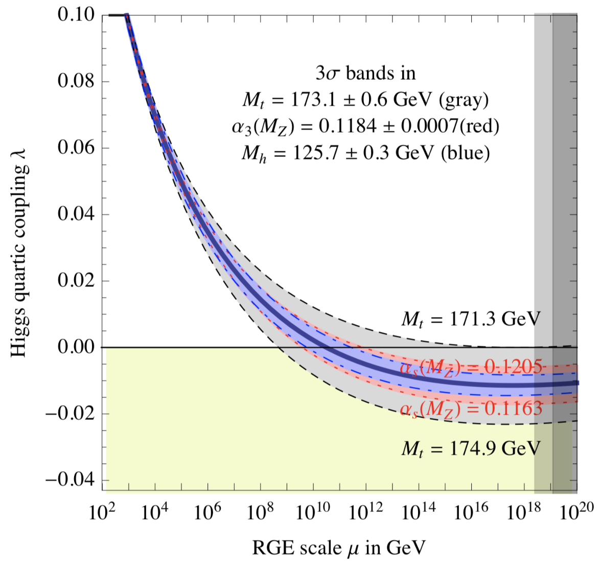
The Higgs quartic coupling is modified only logarithmically by loop corrections, but the effect of running to high energy can be dramatic. At leading order, and neglecting small contribtions from the gauge couplings, the renormalization group running of is given by the following expression:
| (3) |
where is the top Yukawa coupling, and is the running Higgs selfcoupling. It is straightforward to verify that, for the actual values of the top and Higgs masses, , and is driven to smaller values at large . A complete analysis, including higher order terms (see e.g. [26]), indicates that turns negative at energies in the range of GeV, as shown in Fig. 1. A negative would make the potential unstable, and short-distance quantum fluctuations could therefore potentially destabilize the SM Higgs vacuum. The timescale for “our” vacuum to run away, calculated with the given values of top and Higgs mass, is much longer than the age of the universe, making the vacuum metastable and consistent with observation [27]. But it is disturbing, once more, that the dynamics of the Higgs field be influenced so much by physics taking place at scales much higher than the weak scale!
Both the puzzle of the hierarchy problem and the issue of the metastability of the Higgs vacuum point to the existence of a more fundamental layer behind EW symmetry breaking, and galvanise the need to understand the deeper origin of the Higgs potential.
2.2 More exploration targets for future colliders
Even setting to the side the key issue of the origin of the Higgs, there are other very concrete reasons why the Higgs deserves further study, and may provide a window to undiscovered phenomena. As it carries no spin and is electrically neutral, the Higgs may have so-called ‘relevant’ (i.e. dimension-4) interactions (e.g. ) with a scalar particle, S, living in sectors of particle physics that are otherwise totally decoupled from the SM interactions. These interactions, even if they only take place at very high energies, remain relevant at low energies – contrary to interactions between new neutral scalars and the other SM particles. The possibility of new hidden sectors already has strong experimental support: there is overwhelming evidence from astrophysical observations that a large fraction of the observed matter density in the universe is invisible. This so-called dark matter (DM) makes up 26% of the total energy density in the universe and more than 80% of the total matter [28]. Despite numerous observations of the astrophysical properties of DM, not much is known about its particle nature. This makes the discovery and identification of DM one of the most pressing questions in science, a question whose answer may hinge on the role of the Higgs boson.
The current main constraints on a particle DM candidate are that it: a) should gravitate like ordinary matter, b) should not carry colour or electromagnetic charge, c) is massive and non-relativistic at the time the CMB forms, d) is long lived enough to be present in the universe today (), and e) does not have too strong self-interactions (). While no SM particles satisfy these criteria, they do not pose very strong constraints on the properties of new particles to play the role of DM. In particular the allowed range of masses spans almost 80 orders of magnitude. Particles with mass below eV would have a wave length so large that they wipe out structures on the kPc (kilo-Parsec) scale and larger [29], disagreeing with observations, while on the other end of the scale micro-lensing and MACHO (Massive Astrophysical Compact Halo Objects) searches put an upper bound of solar masses or GeV on the mass of the dominant DM component [30, 31, 32]. We shall discuss later on how future colliders can attack this pressing question, providing comprehensive exploration of the class of ‘thermal freeze-out’ DM, which picks out a particular broad mass range as a well-motivated experimental target, as well as unique probes of weakly coupled dark sectors.
Returning to the matter which is observable in the Universe, the SM alone cannot explain baryogenesis, namely the origin of the dominance of matter over antimatter that we observe today. Since the matter-antimatter asymmetry was created in the early universe when temperatures and energies were high, higher energies must be explored to uncover the new particles responsible for it, and the LHC can only start this search. In particular, a well-motivated class of scenarios, known as EW baryogenesis theories, can explain the matter-antimatter asymmetry by modifying how the transition from the high-temperature EW-symmetric phase to the low-temperature symmetry-broken phase occurred. Independently of the problem of the matter-antimatter asymmetry, there is the question of the nature of the EW phase transition (EWPT): was it a smooth cross-over, as predicted by the SM, or a first-order one, as possible in BSM scenarios (and as necessary to enable EW baryogenesis)? Since this phase transition occurred at temperatures near the weak scale, the new states required to modify the transition would likely have mass not too far above the weak scale, singling out future 100 TeV colliders as the leading experimental facility to explore the nature of this foundational epoch of the early Universe.
Another outstanding question lies in the origin of the neutrino masses, which the SM alone cannot account for. As with DM, there are numerous models for neutrino masses that are within the discovery reach of future lepton and hadron colliders, as discussed in Ref. [9].
These and other outstanding questions might also imply the existence of further spatial dimensions, or larger symmetries that unify leptons and quarks or the known forces. The LHC’s findings notwithstanding, higher energy and larger statistics will be needed to explore these fundamental mysteries more deeply and possibly reveal new paradigm shifts.
3 The way forward with future colliders
Since the mid 70’s, the path to establish experimentally the SM was clear: discover the gauge bosons and complete the fermion sector (e.g. determine the number of SM-like neutrino species and eventually discover the top quark), test strong and EW interactions at the level of quantum corrections (comparing precise measurements and accurate theoretical predictions), test the CKM framework of flavor phenomena, and discover the Higgs boson. Having accomplished all this, the situation today is less well defined. In spite of the fact that the formulation of the open problems, as reviewed in the previous Section, is rather clear, there is however no experimental approach known today that can guarantee conclusive answers. This is underscored by the fact that our prejudices on where to look have not given results. One of the main questions we face in planning our future is therefore “why don’t we see as yet any sign of the new physics that we confidently expected to be present around the TeV scale?”. The question admits two possible answers: (i) the mass scale of the new physics lies beyond the LHC reach, or, (ii) while being within LHC’s reach, its manifestations are elusive and escaped so far the direct search. These two scenarios are a priori equally likely, but they clearly impact in different ways the future of our field, and thus the assessment of the physics potential of possible future facilities. Our safest hedge is therefore the readiness to cover both scenarios, via an experimental programme relying on higher precision and sensitivity (to address possible elusive signatures), and on an extended energy and mass reach relative to the LHC.
A possible way to assess the value of a future collider facility is to consider the following three criteria:
- •
The guaranteed deliverables. This criterion is what I refer to as the “value of measurements”: the new information that we can collect to probe the SM to a deeper level, pushing further the exploration of particles and processes that are still poorly known. The main targets of this component of the programme include of course the Higgs boson, the gauge bosons and EW interactions at energies above the EWSB scale, the flavor phenomena, in particular those related to the least known fermions, such as the top quark or the tau lepton.
- •
The discovery potential. While the emergence of phenomena beyond the SM cannot be guaranteed, a future facility must promise a significant extension of today’s sensitivity to new physics, addressing the most relevant and compelling BSM scenarios under consideration, and with sufficient flexibility to accommodate new ideas. The increase in the reach for direct discovery at the highest masses should be accompanied by the increased sensitivity throughout the whole mass range, thanks to higher precision and statistics. The mass reach for direct discovery should ideally match the sensitivity reach obtained indirectly via precision measurements.
- •
Conclusive answers. Unless an actual discovery is made, no experiment can provide conclusive answers to general questions such as “what is DM?”, “do supersymmetry or new Z’ bosons exist?”. Lack of evidence can be evaded by pushing the relevant mass spectrum beyond reach. But there exist important, less generic, questions, for which it is reasonable to expect that a conclusive answer can be found below well-defined mass scales. Some examples were given before: did EWSB induce a first order phase transition? Is DM made of particles coupled to the SM via the weak interaction? Do neutrino masses arise from the weak scale? Even negative answers, if firm, would be of great value, since they would force us to focus the searches elsewhere. While current experiments (LHC and others) could find partial answers, conclusive statements are expected to require higher energy and sensitivity, setting performance targets for the evaluation of future experiments.
These lectures will present an overview of the physics potential of the various elements of the FCC programme, in the light of those three criteria.
3.1 The Role of FCC-ee
The capabilities of circular colliders are well illustrated by LEP, which occupied the LHC tunnel from 1989 to 2000. Its point-like collisions between electrons and positrons and precisely known beam energy allowed the four LEP experiments to test the SM to new levels of precision, particularly regarding the properties of the W and Z bosons. Putting such a machine in a 100 km tunnel and taking advantage of advances in accelerator technology such as superconducting radio-frequency cavities would offer even greater levels of precision on a greater number of processes. For example, it would be possible to adapt the collision energy during about 15 years of operation, to examine physics at the Z pole, at the WW production threshold, at the peak of ZH production, and above the threshold. Controlling the beam energy at the 100 keV level would allow exquisite measurements of the Z and W boson masses, whilst collecting samples of up to Z and W bosons, not to mention several million Higgs bosons and top quark pairs. The experimental precision would surpass any previous experiment and challenge cutting edge theory calculations.
FCC-ee would quite literally provide a quantum leap in our understanding of the Higgs. Like the W and Z gauge bosons, the Higgs receives quantum EW corrections typically measuring a few per cent in magnitude due to fluctuations of massive particles such as the top quark. This aspect of the gauge bosons was successfully explored at LEP, but now it is the turn of the Higgs – the keystone in the EW sector of the SM. The millions of Higgs bosons produced by FCC-ee, with its clinically precise environment, would push the accuracy of the measurements to the per mille level, accessing the quantum underpinnings of the Higgs and probing deep into this hitherto unexplored frontier. In the process , the mass recoiling against the Z has a sharp peak that allows a unique and absolute determination of the Higgs decay-width and production cross section. This will provide an absolute normalisation for all Higgs measurements performed at the FCC, enabling exotic Higgs decays to be measured in a model independent manner.
The high statistics promised by the FCC-ee programme goes far beyond precision Higgs measurements. Other signals of new physics could arise from the observation of flavour changing neutral currents or lepton-flavour-violating decays, by the precise measurements of the Z and H invisible decay widths, or by direct observation of particles with extremely weak couplings, such as right-handed neutrinos and other exotic particles. The precision of the FCC-ee programme on EW measurements would allow new physics effects to be probed at scales as high as 100 TeV, anticipating what the FCC-hh must focus on.
3.2 The Role of FCC-hh and FCC-eh
The FCC-hh would operate at seven times the LHC energy, and collect about 10 times more luminosity. The discovery reach for high-mass particles – such as Z′ or W′ gauge bosons corresponding to new fundamental forces, or gluinos and squarks in supersymmetric theories – will increase by a factor five or more, depending on the final statistics. The production rate of particles already within the LHC reach, such as top quarks or Higgs bosons, will increase by even larger factors. During the planned 25 years of data taking, a total of more than Higgs bosons will be created, several thousand times more than collected by the LHC through Run 2 and 200 times more than will be available by the end of its operation. These additional statistics will enable the FCC-hh experiments to improve the separation of Higgs signals from the huge backgrounds that afflict most LHC studies, overcoming some of the dominant systematics that limit the precision attainable at the LHC. While the ultimate precision of most Higgs properties can only be achieved with FCC-ee, several demand complementary information from FCC-hh. For example, the direct measurement of the coupling between the Higgs and the top quark requires that they be produced together, requiring an energy beyond the reach of the FCC-ee. At 100 TeV, almost out of the top quarks produced will radiate a Higgs boson, allowing the top-Higgs interaction to be measured at the 1% level – several times better than at the HL-LHC and probing deep into the quantum structure of this interaction. Similar precision can be reached for Higgs decays that are too rare to be studied in detail at FCC-ee, such as those to muon pairs or to a Z and a photon. All of these measurements will be complementary to those obtained with FCC-ee and will use them as reference inputs to precisely correlate the strength of the signals obtained through various production and decay modes.
One respect in which a 100 TeV proton-proton collider would really come to the fore is in revealing how the Higgs behaves in private. The rate of Higgs pair production events, which in some part occur through Higgs self-interactions, would grow by a factor of 40 at FCC-hh, with respect to 14 TeV, and enable this unique property of the Higgs to be measured with an accuracy reaching 5%. Among many other uses, such a measurement would comprehensively explore classes of models that rely on modifying the Higgs potential to drive a strong first order phase transition at the time of EW symmetry breaking, a necessary condition to induce baryogenesis.
FCC-hh would also allow an exhaustive exploration of new TeV-scale phenomena. Indirect evidence for new physics can emerge from the scattering of W bosons at high energy – where the Higgs boson plays a key role in controlling the rate growth – from the production of Higgs bosons at very large transverse momentum, or by testing the far ‘off-shell’ nature of the Z boson via the measurement of lepton pairs with invariant masses in the multi-TeV region. The plethora of new particles predicted by most models of symmetry-breaking alternatives to the SM can be searched for directly, thanks to the immense mass reach of 100 TeV collisions. The search for DM, for example, will cover the possible space of parameters of many theories relying on weakly interacting massive particles, guaranteeing a discovery or ruling them out. Several theories that address the hierarchy problem will also be conclusively tested. For supersymmetry, the mass reach of FCC-hh pushes beyond the regions motivated by the hierarchy problem alone. For composite Higgs theories, the precision Higgs coupling measurements and searches for new heavy resonances will fully cover the motivated territory. A 100 TeV proton collider will even confront exotic scenarios such as the twin Higgs, which are extremely difficult to test. These theories predict very rare or exotic Higgs decays, possibly visible at FCC-hh thanks to its enormous Higgs production rates.
The FCC-eh collider could operate in synchronous, symbiotic operation alongside the pp collider. The facility would serve as the most powerful, high-resolution microscope onto the substructure of matter ever built. High-energy ep collisions would provide precise information on the quark and gluon structure of the proton, and how they interact. FCC-eh would complement and enhance the study of the Higgs, and broaden the new physics searches also performed at FCC-hh and FCC-ee, with a specific focus on phenomena such as quark substructure, leptoquarks, heavy sterile neutrinos and long-lived particles.
While not discussed at all in these lectures, FCC-hh would also enable the continuation of the LHC successful programme of heavy ion collisions, extending studies of the thermodynamic behaviour of QCD of crucial relevance to multiple topics, ranging from the fundamental properties of quantum field theory, to cosmology and astrophysics.
4 Higgs boson properties
Indirect information about the Higgs boson is accessible through precision EW measurements, as proven by the global fits to the LEP and SLC data, which set very tight constraints on the Higgs mass well before its discovery. But, following the Higgs discovery, the most direct way to test the Higgs properties is to produce it and observe its decay features. With the knowledge of the Higgs mass, the SM predicts uniquely its couplings to each SM particle, and therefore all production and decay rates are fixed. Since our target is to explore the origin of EWSB, and possibly identify the underlying BSM phenomena that trigger it, we must be open however to all sorts of deviations from the SM. For example, while the couplings of the Higgs to the gauge bosons are determined by the Higgs quantum numbers (an SU(2) doublet), the existence of an additional Higgs scalar, acquiring its own expectation value, could lead to a mixing in the Higgs sector, and the mass eigenstate at 125 GeV could couple to the W and the Z with a slightly reduced strength. The existence of additional Higgses opens the door to the possibility that different fermions couple to different Higgses, modifying the direct relation between fermion mass and Yukawa coupling to the 125 GeV state (as in the case in supersymmetry). The study of Higgs couplings, threfore, requires as much as possible a model independent approach.
Establishing the gauge couplings of the known fermions was relatively straightforward, since they are quantized and the fermion assignment to a gauge group representation ranges over a discrete set of possibilities. Deviations are possible of course, but only in presence of additional BSM interactions, that appear at low energy as operators of dimension higher than 4. The basic, leading-order and renormalizable interactions of SM fermions are therefore easily established experimentally. That the top quark is an color triplet, for example, can follow from the analysis of its production rate and decay patterns11 1 This is so straightforward in principle, that I am not even sure there has ever been an explicit experimental analysis to confirm that the top quark is a triplet. I leave it to you as an exercise to list the data and signatures that could be used to confirm it.. On the contrary, the leading-order Higgs couplings are a priori a generic real (or complex) number, and the confidence on whether they agree or not with the SM will always only be conditional to the precision of the available data.

The dominant Higgs production channels, in hadronic collisions like at the LHC, are shown in Fig. 2. In these examples, the production rates are proportional to the coulings to the gauge bosons, or to the top quark. In the ideal world in which the strong coupling , the partonic densities (PDFs) and the QCD matrix elements were perfectly known, counting events in a given decay mode would provide a measurement of , where are the Higgs couplings to initial and final state state, and () is the partial (total) decay width. If we could observe every possible Higgs decay, summing over all Y states for a given production channel X would allow the measurement of , since . At the LHC and in general in hadronic collisions, this is hardly possible: several SM decay modes with a substantial branching ratio (BR), like , are very difficult to measure, and possible exotic Higgs decays are also likely to escape detection. A completely model-independent extraction of Higgs couplings in hadronic collisions can therefore only reach a limited precision, independently of the theoretical challenge of properly calculating the QCD part of the reactions.
As we show in the next sections, the measurements at an electron collider can provide the needed input of , and open the way for a powerful synergetic programme of precision measurements with the next generation of hadron colliders.
A complete compilation and critical review of the Higgs coupling measurement prospects covering all proposed future colliders can be found in Ref. [33].
4.1 Higgs coupling measurements at FCC-ee


The determination of is however possible at future colliders, operating above the ZH threshold. Here, the production of a Higgs boson can be reconstructed, in a model-independent way, with the so-called recoil-mass technique. One considers final states, and for each event defines the recoil mass as . Most final states arise from ZZ production (), in which case is the momentum of the second Z, and the recoil mass equals (up to finite-width and experimental resolution effects) the Z mass. A further contribution comes from WW production (), in which case represents the missing momentum, and the recoil mass is a broad continuum. In the case of production (see the left image of Fig. 3), the recoil mass coincides with the Higgs mass, regardless of the H decay mode. These three contributions are shown, for the simulation of an FCC-ee experiment, in Fig. 3. A global fit of the recoil mass spectrum returns the total number of Higgs produced in , and a direct measurement of the HZZ coupling, . If we now focus on events with the decay, and consider that their rate is proportional to , the knowledge of allows to extract in a model-independent way.
Exercise: discuss, in a qualitative way, to which extent EW
radiative corrections or BSM effects influence this line of reasoning, and whether
they affect the “model-independent” argument.
Exercise: discuss, in a qualitative way, the backgrounds under
the H peak in the recoil mass spectrum, and how they can be estimated,
and subtracted, precisely.
Exercise: discuss how the recoil mass observable can be used to
determine the presence of exotic (in particular, invisible) H decays.
Having established the value of , further dedicated measurements allow to determine the absolute value of the Higgs couplings to all particles accessible via decay modes or production channels. Assuming SM couplings, the statistical precision that can be achieved for several BRs measurable at FCC-ee is summarized in Table 1 (for the details of the reconstruction of individual final states, see e.g. [10]). These include the results obtained from the run just above the Higgs threhsold, at 240 GeV, and the runs above the thresholds, where the VBF process , shown in Fig. 4, becomes relevant.


| (GeV) | ||||
|---|---|---|---|---|
| Luminosity () | 5 | |||
| (%) | HZ | ν H | HZ | ν H |
| ττ | ||||
| γγ | ||||
| µ+µ- | ||||
| Collider | HL-LHC | FCC-ee240+365 | ||
|---|---|---|---|---|
| Lumi () | 3 | HL-LHC | ||
| Years | 25 | 3 | 4 | |
| (%) | SM | 2.7 | 1.3 | 1.1 |
| (%) | 1.5 | 0.2 | 0.17 | 0.16 |
| (%) | 1.7 | 1.3 | 0.43 | 0.40 |
| (%) | 3.7 | 1.3 | 0.61 | 0.56 |
| (%) | SM | 1.7 | 1.21 | 1.18 |
| (%) | 2.5 | 1.6 | 1.01 | 0.90 |
| (%) | 1.9 | 1.4 | 0.74 | 0.67 |
| (%) | 4.3 | 10.1 | 9.0 | 3.8 |
| (%) | 1.8 | 4.8 | 3.9 | 1.3 |
| (%) | 3.4 | – | – | 3.1 |
| BREXO (%) | SM | |||
In practice, the width and the couplings are determined with a global fit, which closely follows the logic of Ref. [35]. The results of this fit are summarised in Table 2 and are compared to the same fit applied to HL-LHC projections [34]. Table 2 also shows that the extractions of and of from the global fit are significantly improved by the addition of the WW-fusion process at GeV, as a result of the correlation between the HZ and ν H processes. In particular the Higgs EW couplings have a permille-level precision, and the couplings to the tau, the bottom and charm quarks and the effective couplng to the gluon reach the percent level or better.
Several SM couplings are left out of these projections: to the lightest quarks (u, d, s), to the electron, to the top quark, to the pair, and the Higgs self-coupling. To access the light quarks, several ideas have been proposed: exclusive decays to hadronic resonances, such as (, V=W/Z/γ) [36, 37, 38, 39], light-jet tagging techniques [40], or kinematical distributions of the Higgs boson in hadronic collisions [41, 42]. Experimental searches for exclusive radiative hadronic decays have started already at the LHC [43], to at least establish upper limits, even though well beyond the SM expectations. Given the small BRs, an electron collider will barely have sufficient statistics to gain the required SM sensitivity. At the FCC-ee, the most promising channel is Hγρ[ππ], with about 40 events expected [44]. A future hadron collider will have much more events to play with, but backgrounds and experimental conditions will be extremely challenging, and only detailed simulations will be able to establish their true potential.
To probe the Hee coupling, the best hope appears to be the direct resonant production in . The low rate demands high luminosity, and a tuning of the beam energy to exactly match . Preliminary studies [44] indicate that a 3 observation requires an integrated luminosity of 90ab-1, namely several years of dedicated running at 125 GeV.
While the direct access to the Htt coupling in an collider requires a center-of-mass energy of 500 GeV and more, FCC-ee will expose an indirect sensitivity to it, through its effect at quantum level on the cross section just above production threshold, GeV. The precise measurement of from the runs at the Z pole will allow the QCD effects to be disentangled from those of the top Yukawa coupling at the vertex, to achieve a precision of [10].
To access in a direct way the top Yukawa coupling, and to improve to the percent level the measurement of small BR decays such as Hγγ, Zγ and µ+µ-, we can then appeal to the huge statistics available to a hadron collider.
4.2 Higgs couplings measurements at FCC-hh
Two elements characterise Higgs production at the FCC-hh: the large statistics (see Table 3), and the large kinematic range, which, for several production channels, probes in the multi-TeV region (see Fig. 5).
| ggH | VBF | WH | ZH | tt̄H | HH | |
|---|---|---|---|---|---|---|
| 180 | 170 | 100 | 110 | 530 | 390 | |
| 16 | 15 | 11 | 12 | 24 | 19 |
These factors lead to an extended and diverse sensitivity to possible deviations of the Higgs properties from their SM predictions: the large rates enable precise measurements of branching ratios for rare decay channels such as γγ or µµ, and push the sensitivity to otherwise forbidden channels such as τµ. The large kinematic range can be used to define cuts improving the signal-to-background ratios and the modelling or experimental systematics, but it can also amplify the presence of modified Higgs couplings, described by higher-dimension operators, whose impact grows with . Overall, the Higgs physics programme of FCC-hh is a fundamental complement to what can be measured at FCC-ee, and the two Higgs programmes greatly enrich each other. This section contains some examples of these facts, and documents the current status of the precision projections for Higgs measurements. A more extensive discussion of Higgs production properties at 100 TeV and of possible measurements is given in Ref. [45].
Figure 5 shows the Higgs rates above a given threshold, for various production channels. It should be noted that these rates remain above the level of one million up to TeV, and there is statistics for final states like Hbb̄ or Hττ extending up to several TeV. Furthermore, for 1 TeV, the leading production channel becomes tt̄H, followed by vector boson fusion when 2 TeV. The analysis strategies to separate various production and decay modes in these regimes will therefore be different to what is used at the LHC. Higgs measurements at 100 TeV will offer many new options and precision opportunities with respect to the LHC, as it happened with the top quark moving from the statistics-hungry Tevatron to the rich LHC.
Exercise: discuss possible strategies to separate the different
Higgs production processes in the various ranges of shown in
Fig. 5.
For example, as shown in Ref. [45], improves for several final states at large . In the case of the important γγ final state, Fig. 6 shows that increases from at low (a value similar to what observed at the LHC), to at GeV. In this range of few hundred GeV, some experimental systematics will also improve, from the determination of the energies (relevant e.g. for the mass resolution of Hγγ or bb̄) to the mitigation of pile-up effects.
Exercise: why do you think S/B improves at
large for a process like γγ]+jet?
The analyses carried out so far for FCC-hh are still rather crude when compared to the LHC standards, but help to define useful targets for the ultimate attainable precision and the overall detector performance. The details of the present detector simulations for Higgs physics at FCC-hh are contained in Ref. [46].
The target uncertainties considered include statistics (taking into account analysis cuts, expected efficiencies, and the possible irreducible backgrounds) and systematics (limited here to the identification efficiencies for the relevant final states, and an overall 1% to account for luminosity and modelling uncertainties). While these estimates do not reflect the full complexity of the experimental analyses in the huge pile-up environment of FCC-hh, the systematics assumptions that were used are rather conservative. Significant improvements in the precision of reconstruction efficiencies would arise, for example, by applying tag-and-probe methods to large-statistics control samples. Modelling uncertainties will likewise improve through better calculations, and broad campaigns of validation against data. By choosing here to work with Higgs bosons produced at large , the challenges met by triggers and reconstruction in the high pile-up environment are eased. The projections given here are therefore considered to be reasonable targets for the ultimate precision, and useful benchmarks to define the goals of the detector performance.
The consideration of the reconstruction efficiency of leptons and photons is relevant in this context since, to obtain the highest precision by removing global uncertainties such as luminosity and production modelling, ratios of different decay channels can be exploited. The reconstruction efficiencies are shown in Fig. 7 as a function of . The uncertainties on the electron and photon efficiencies are assumed to be fully correlated, but totally uncorrelated from the muon one. The curves in Fig. 7 reflect what is achievable today at the LHC, and it is reasonable to expect that smaller uncertainties will be available at the FCC-hh, due to the higher statistics that will allow statistically more powerful data-driven fine tuning. For example, imposing the identity of the Z boson rate in the ee and µµ decay channels will strongly correlate the e and µ efficiencies.
The absolute uncertainty expected in the measurement of the production and decay rates for several final states is shown in Fig. 8, as a function of the minimum . The curves labeled by “stat+syst” include the optimal reconstruction efficiency uncertainties shown in Fig. 7. The curves labeled by “stat+syst+lumi” include a further 1%, to account for the overall uncertainty related to luminosity and production systematics. The luminosity itself could be known even better than that by using a standard candle process such as Z production, where both the partonic cross section and the PDF luminosity will be pinned down by future theoretical calculations, and by the FCC-eh, respectively. Notice that the gg luminosity in the mass range between and several TeV will be measured by FCC-eh at the few per mille level.
Several comments on these figures are in order. First of all, it should be noted that the inclusion of the systematic uncertainty leads to a minimum in the overall uncertainty for values in the range of few hundred GeV. The very large FCC-hh statistics make it possible to fully benefit from this region, where experimental systematics are getting smaller. The second remark is that the measurements of the Higgs spectrum can be performed with a precision better than 10%, using very clean final states such as γγ and 4, up to values well in excess of 1 TeV, allowing the possible existence of higher-dimension operators affecting Higgs dynamics to be probed up to scales of several TeV.
Independently of future progress, the systematics related to production modelling and to luminosity cancel entirely by taking the ratio of different decay modes, provided selection cuts corresponding to identical fiducial kinematic domains for the Higgs boson are used. This can be done for the final states considered in Fig. 8. Ratios of production rates for these channels provide absolute determinations of ratios of branching ratios, with uncertainties dominated by the statistics, and by the uncorrelated systematics such as reconstruction efficiencies for the different final state particles. These ratios are shown in Fig. 9. The curves with the systematics labeled as “cons” use the conservative reconstruction uncertainties plotted in Fig. 7.
| Observable | Parameter | Precision | Precision |
|---|---|---|---|
| (stat) | (stat+syst+lumi) | ||
| (H)B(H γγ) | 0.1% | 1.5% | |
| (H) B(Hµµ) | 0.28% | 1.2% | |
| (H)B(H 4µ) | 0.18% | 1.9% | |
| (H)B(H γµµ) | 0.55% | 1.6% | |
| (HH)B(Hγγ)B(Hbb̄) | 5% | 7.0% | |
| B(Hµµ)/B(H4µ) | 0.33% | 1.3% | |
| B(Hγγ)/B(H 2e2µ) | 0.17% | 0.8% | |
| B(Hγγ)/B(H 2µ) | 0.29% | 1.4% | |
| B(Hµµγ)/B(Hµµ) | 0.58% | 1.8% | |
| (tt̄H) B(H bb̄)/(tt̄Z)B(Z bb̄) | 1.05% | 1.9% | |
| (H invisible) | 95%CL |
These results are summarised in Table 4, separately showing the statistical and systematic uncertainties obtained in our studies. As remarked above, there is in principle room for further progress, by fully exploiting data-driven techniques to reduce the experimental systematics. At the least, one can expect that these potential improvements will compensate for the current neglect of other experimental complexity, such as pile-up. The most robust measurements will involve the ratios of branching ratios. Taking as a given the value of the HZZ coupling (and therefore (H)), which will be measured to the few per-mille level by FCC-ee, from the FCC-hh ratios it could be possible to extract the absolute couplings of the Higgs to γγ (0.4%), µµ (0.7%), and Zγ(0.9%).
Exercise: discuss the possible role of precise measurememts of
ratios of BRs in exploring the microscopic origin of potential
deviations from the SM expectations. Which type of models can give
rise to deviations in the ratios considered here? Which models would
leave no signatures in these ratios?
The ratio with the tt̄Z process is considered for the tt̄H process, as proposed in Ref. [47]. This allows the removal of the luminosity uncertainty, and reducing the theoretical systematics on the production modelling below 1%. An updated study of this process, including the FCC-hh detector simulation, is presented in Ref. [46]. Assuming FCC-ee will deliver the expected precise knowledge of (Hbb̄), and the confirmation of the SM predictions for the Ztt̄ vertex, the tt̄H/tt̄Z ratio should therefore allow a determination of the top Yukawa coupling to 1%.
The limit quoted in Table 4 on the decay rate of the Higgs boson to new invisible particles is obtained from a study of large missing- signatures. The analysis, discussed in detail in Ref. [46], relies on the data-driven determination of the leading SM backgrounds from W/Z+jets. The integrated luminosity evolution of the sensitivity to invisible H decays is shown in Fig. 10. The SM decay H4ν, with branching ratio of about , will be seen after 1 ab-1, and the full FCC-hh statistics will push the sensitivity to .
Exercise: if the Higgs admits an important decay rate to non-SM
particles, will increase. A larger width will reduce all BRs by a
common factor. Assuming that these decay signatures are elusive in a
hadron collider, discuss how ratios of BRs could still be used to learn
more about their origin.
Last but not least, Table 4 reports a 7% expected precision in the extraction of the Higgs self-coupling . This result is discussed in more detail in a later Section, with other probes of the Higgs self-interaction.
| cut | GeV | GeV | GeV | GeV |
|---|---|---|---|---|
| [0.98,1.05] | [0.99,1.04] | [0.99,1.03] | [0.98,1.02] |
4.3 Longitudinal Vector Boson Scattering
The scattering of the longitudinal components of vector bosons is particularly sensitive to the relation between gauge couplings and the VVH coupling. A thorough analysis of same-sign scattering, in the context of the FCC-hh detector performance studies, is documented in Ref. [46]. The extraction of the signal requires the removal of large QCD backgrounds (+jets, WZ+jets) and the separation of large EW background of transverse-boson scattering. The former is suppressed by requiring a large dilepton invariant mass and the presence of two jets at large forward and backward rapidities. The longitudinal component is then extracted from the scattering of transverse states by exploiting the different azimuthal correlations between the two leptons. The precision obtained for the measurement of the cross section as a function of integrated luminosity, is shown in Fig. 11 (left). The three curves correspond to different assumptions about the rapidity acceptance of the detector and drive the choice of the detector design, setting a lepton (jet) acceptance out to . The small change in precision when increasing the jet cut from to GeV indicates a strong resilience of the results against the presence of large pile-up. The quoted precision, reaching the value of 3% at 30 ab-1, accounts for the systematic uncertainties of luminosity (1%), lepton efficiency (0.5%), PDF (1%) and the shape of the distributions used in the fit (10%). The right plot in Fig. 11 shows the impact of rescaling the WWH coupling by a factor . The effect is largest at the highest dilepton invariant masses, as expected. The measurement precision, represented by the small vertical bars, indicates a sensitivity to at the percent level, as shown also in Table 5.
5 Precision EW measurements
The Higgs boson forms an integral part of the EW sector, and its properties are deeply intertwined with those of EW phenomena. A thorough program of EW measurements goes hand in hand with the study of Higgs properties, and is an essential complement to it. At the FCC, EW interactions can be studied from multiple perspectives, extending by large factors all previous targets of precision and energy reach. We summarize here the main results from the existing studies, documented in more detail in Ref. [9, 10].
The FCC-ee run at the peak will deliver about times the LEP statistics, with about or final states, and hadronic decays. The larger statistics w.r.t. LEP will be accompanied by significant efforts to minimize the systematic uncertainties. For example, the beam energies will be measured more precisely, and better detectors will improve the efficiency of b-tagging or the precision in the absolute luminosity determination. Significant theoretical improvements in the calculation of higher-loop EW and QCD corrections are also foreseen, and necessary to fully exploit the potential improvement by over two orders of magnitude in the statistical precision.
is a crucial input parameter to interpret SM precision observables. The EM coupling at the scale of the electron mass is the best known fundamental constant of nature, but its renormalization group evolution to the scale of weak interactions is subject to important uncertainties, due to non-perturbative hadronic physics, which enters the photon self-energy corrections as evolves through the region of the hadronic resonances. The systematic uncertainties of the experimental data on hadrons end up dominating the precision of the extrapolation to , which is limited to the level of . Dedicated runs at =87.7 and 93.9 GeV will extract directly (namely without an extrapolation in ) from the energy-dependence of the forward-backward asymmetry, improving the current uncertainty by a factor of 4.
Forward-backward and polarization asymmetries will also allow to reduce by a factor of 30-50 the uncertainty in . I recall that today’s determination of the weak mixing angle, [48], is dominated by the combination of two precise measurements (the b-quark forward-backward asymmetry from LEP and the left-right polarization asymmetry from SLD), which differ among themselves by 3.2 standard deviations. While future HL-LHC data [49] will provide an independent determination of the weak mixing angle with a precision approaching the current LEP/SLD one, using the lepton charge asymmetry in Z boson decays, it is only with the future FCC-ee data that this puzzling result will be clarified.
The Z-decay asymmetries will also help improving the measurement of vector and axial couplings of the leptons and of the charm and bottom quarks. In absence of a reliable technique to distinguish Z decays to the different lighter quarks (u, d and s), the most precise determination of their couplings to the neutral current will come from FCC-eh. There, a simultaneous fit to the light quarks EW couplings and to the PDFs, using both charged and neutral current data, will disentangle the individual quarks and allow the measurement of their respective vector and axial couplings. The projection in in Fig. 12 for the precision of all fermionic couplings, from a global fit [50, 51] to both FCC-ee and FCC-eh data treating each lepton and quark flavour as independent, shows the improvement expected with respect to today’s knowledge.

The measurement of the total Z width , and of its visible fraction, will allow to extract the invisible component of . Today, the number of neutrino species obtained from the LEP data is , which is low by two standard deviations. A deficit in the neutrino counting from Z decays could be attributed to a violation of unitarity in the neutrino mixing matrix, or to the presence of right-handed neutrinos [52]. FCC-ee will improve the precision on by almost a factor of 10, down to 0.001.
The pairs of W bosons produced at the two energies of 157.5 and 162.5 GeV will reduce the uncertainty on the W mass, , to 0.5 MeV, and of its width to 1.2 MeV. The limited statistics of W bosons from LEP2 left us with a puzzling discrepancy between the decay branching ratio of the W to the tau lepton, , and to the e and µ( and , resp.). FCC-ee can reduce these uncertainties by almost two orders of magnitude, greatly increasing the sensitivity to possible violations of lepton flavour universality, a topic that is receiving great attention nowadays. For comparison, the Z decays to individual leptons will allow to test neutral-current lepton universality at the level of of . τ semileptonic decays, and the τ lifetime, could achieve a sensitivity to deviations from lepton flavour universality in weak charged currents at a similar level.

A collection of the various EW precision measurements possible at the FCC-ee, including those relative to the top quark properties, is shown in Table 6. Their overall impact in testing the SM relation between the top and W masses is shown in Fig. 13.
| Observable | present | FCC-ee | FCC-ee | Comment and | ||
| value | error | Stat. | Syst. | dominant exp. error | ||
| 91186700 | 2200 | 5 | 100 | From Z line shape scan | ||
| Beam energy calibration | ||||||
| 2495200 | 2300 | 8 | 100 | From Z line shape scan | ||
| Beam energy calibration | ||||||
| 20767 | 25 | 0.06 | 0.2-1.0 | ratio of hadrons to leptons | ||
| acceptance for leptons | ||||||
| 1196 | 30 | 0.1 | 0.4-1.6 | from above [54] | ||
| 216290 | 660 | 0.3 | ¡60 | ratio of to hadrons | ||
| stat. extrapol. from SLD [55] | ||||||
| (nb) | 41541 | 37 | 0.1 | 4 | peak hadronic cross-section | |
| luminosity measurement | ||||||
| 2991 | 7 | 0.005 | 1 | Z peak cross sections | ||
| Luminosity measurement | ||||||
| 231480 | 160 | 3 | 2 - 5 | from at Z peak | ||
| Beam energy calibration | ||||||
| 128952 | 14 | 4 | small | from off peak [56] | ||
| 992 | 16 | 0.02 | 1-3 | b-quark asymmetry at Z pole | ||
| from jet charge | ||||||
| 1498 | 49 | 0.15 | ¡2 | τ polarisation and charge asymmetry | ||
| τ decay physics | ||||||
| 80350 | 15 | 0.5 | 0.3 | From WW threshold scan | ||
| Beam energy calibration | ||||||
| 2085 | 42 | 1.2 | 0.3 | From WW threshold scan | ||
| Beam energy calibration | ||||||
| 1170 | 420 | 3 | small | from [57] | ||
| 2920 | 50 | 0.8 | small | ratio of invis. to leptonic | ||
| in radiative Z returns | ||||||
| 172740 | 500 | 17 | small | From threshold scan | ||
| QCD errors dominate | ||||||
| 1410 | 190 | 45 | small | From threshold scan | ||
| QCD errors dominate | ||||||
| 1.2 | 0.3 | 0.1 | small | From threshold scan | ||
| QCD errors dominate | ||||||
| 30% | % | small | From run |
5.1 Complementarity of EW and Higgs measurements
The best framework to expose the complementarity between Higgs and EW probes of new physics at large scales, is that of the SM effective field theory (SMEFT [58, 59, 60]). Here one assumes that, as in the SM, the Higgs boson transforms as doublet of , and considers all invariant operators, classified according to their dimension:
| (4) |
At dimension 4, one finds the SM itself. At dimension 5 appear the operators that generate Majorana neutrino masses. At dimension 6 one first finds operators that, parameterizing the low-energy behaviour of new interactions beyond the EW scale, lead to modifications of EW and Higgs observables. Focusing on lepton and baryon-number conserving operators, and assuming flavour universality, leaves a basis of 59 dim-6 operators [59].
Figure 14 shows the constraints that future FCC-ee data can impose on the coefficients of the subset of operators that play a role in the EW and Higgs observables discussed so far. On the EW side, one has the following 10 operators:
| (5) |
where is the Higgs scalar doublet, runs over all the 5 types of SM fermion multiplets, while only refers to the 2 types of SM left-handed fermion doublets. The field can induce effects in processes where an explicit Higgs particle is present, or can influence EW observables indirectly, when is set to its vacuum expectation value. The other 8 operators shown in Fig 14 are mostly affecting Higgs observables:
| (6) |
The sensitivities to the ratios are reported in Fig. 14 as 95 probability bounds on the interaction scale, , associated to each operator. Notice that, in the same way that the energy scale associated to the Fermi constant differs from the W boson mass by a factor related to the weak coupling, the interaction scale defined by does not correspond exactly to the mass of new particles.
Few remarks are in order. First of all, comparison [10] with the current constraints shows that the FCC-ee data will increase by a factor of 4-5 the sensitivity to new energy scales. This matches well the factor of 7 increase in energy of the FCC-hh w.r.t. the LHC, which will lead to a comparable incease in the direct sensitivity to new physics. In other words, a 100 TeV pp collider is typically properly scaled to search for the microscopic orgin of possible deviations observed by the FCC-ee precision measurements. In absolute terms, the scales that can be probed in the case of weakly-interacting new physics () range between a few and few tens of TeV, while they can go up to O(100) TeV in the case of strongly interacting forces. The second remark is that Fig. 14 underscores the complementarity between EW and Higgs observables: even though operators considered here (except ) include both Higgs and gauge bosons or fermions, their constraints come primarily from either EW or Higgs measurements. Both types of measurements are therefore necessary for a systematic exploration of BSM contributions induced via SMEFT operators. The respective scale sensitivity observed for both types of operators is rather consistent, with most limits on interaction scales in the range of 20-30 TeV, showing that the precision targets set by the Higgs and EW programs are coherent.
6 Precision versus sensitivity
In the previous sections, we focused on the very precise measurements that the FCC enables, both in the Higgs and in the EW sector of the SM. These measurements have a value per se, independently of whether we eventually find discrepancies w.r.t. the SM expectations. We need these precise measurements to test up to which point our understanding of fundamental EW phenomena is controlled by the SM. But we also need precise measurements because, the day new physics were found some place, we shall need as much data as possible to evaluate and constrain the many models that will be proposed to explain it. In this context, data that agree with the SM can be as useful as data that may not agree with it. Precise data in agreement with the SM, for example, can help us rule out claims of observations of new physics that were to openly clash with established measurements.
So, the success of a precision physics program is not necessarily tied to the discovery of discrepancies with the SM, but builds on reliable, unbiased and ever more accurate measurements of how nature behaves. Treating the achievable precision as a gauge of the sensitivity to new physics phenomena, however, is critical to examine and characterize the potential relevance of a given measurement in a specific BSM context. It is also a useful way to evaluate the reach of different facilities, which might not measure exactly the same observable: the interpretation of their measurements in terms of constraints on some common BSM phenomenon can be seen as a useful standard candle for their comparison, to assess synergies and complementarities.

In the context of the FCC, there is great richness of synergies and complementarities. The same new physics model can manifest itself via departures in indirect precision measurements at FCC-ee, and directly via the production of new particles at FCC-hh. But low- and high-energy observables can also both participate in building indirect evidence for new phenomena living at scales that are beyond the direct discovery reach. This interplay can be shown with a general example, using the EFT language. Let us consider a dimension-6 operator , parameterizing at energies the effects of some new physics present at a scale . This induces a contribution to the Lagrangian given by , and leads to corrections to the transition between the initial and final states and . By dimensional analysis, will scale, relative to a dimension-4 SM contribution, like , where is a mass scale characteristic of the transition. In the case of a Higgs decay, or of Higgs production at threshold as in , the only possible scales are or . Taking e.g. , gives . If the transition involves another large kinematical scale , with , as in the case of Higgs production at large (see Fig. 15), the deviation could scale like , . The impact of the EFT operator would therefore be greatly enhanced at large . Assuming TeV, for example, a measurements at a scale GeV would lead to an effect of approximatey 15%, ten times larger than for the decay or production at threshold. This means that, at large , one can detect the presence of new physics effects with lesser precision than is required at smaller 22 2 Needless to say the EFT formalism looses validity once the hard scale becomes large enough to induce direct manifestation of new physics. . A hadron collider cannot provide precision comparable to an electron collider, but its higher kinematical reach can compensate for this!
Several studies of this interplay between precision and sensitivity from high-energy indirect measurements have appeared in the literature (see e.g. [61, 62, 63, 64, 65, 66, 67, 68]) covering both Higgs and EW observables. Several of these papers test these ideas in the context of the LHC, and the sensitivity comparison is therefore drawn w.r.t. the LEP precision measurements. We shall give here a couple of examples specific to the 100 TeV collider, where the kinematic reach and the large Higgs production rates make this approach even more powerful.
6.1 Example: the VVHH coupling
Figure 16 shows the diagrams for Higgs-pair production via vector boson fusion, studied in Ref. [69]. At large invariant mass of the Higgs pair, , the triple-Higgs coupling contribution is suppressed by the off-shell Higgs propagator,
and the amplitude is controlled by the behaviour of the longitudinal-longitudinal component of the amplitude, characterised by the destructive interference between the first two diagrams:
| (7) |
Here, and represent, respectively, the coefficients of the VVHH and VVH couplings, normalised to their SM values. vanishes in the SM and in models where the symmetry is linearly realized, and the growth of the amplitude with energy is suppressed. In composite Higgs models based e.g. on an symmetry [70], on the other hand, and (), so the scattering amplitude grows with energy as .
The study of Ref. [69] considered the HH4b final state, applying boosted-jet tagging techniques, given the high of the Higgs bosons at high . The impact of is visible in Fig. 17, which shows the distribution in the SM in a , scenario, and the expected backgrounds. will be measured with a few per-mille precision at FCC-ee (independently of whether it agrees or not with the SM), and the constraints on at FCC-hh will translate directly into a constraint on . The detailed study of Ref. [69] projects a sensitivity to deviations of from its SM value of better than , in spite of the much coarser precision in the measurement of the HH rates! See Ref. [69] for the discussion of the validity range of the EFT approximation.
6.2 Example: Drell-Yan at large mass
Drell-Yan (DY) production is another example where energy can complement precision, achieving sensitivity to new high-scale phenomena [71]. The total production rates of W± and Z0 bosons at 100 TeV are about 1.3 and 0.4 µb, respectively, i.e. samples of leptonic decays per ab-1! A large fraction of these events probe very high energies. Figure 18, left panel, shows the integrated spectra of the W boson transverse mass () and of the γ/Z dilepton mass.
Exercise: The right panel of
Fig. 18 shows the invariant mass spectrum of gauge boson
pairs. Compare these rates to those for lepton-pair production (left
panel), and discuss the reasons for the large differences.
In presence of new physics, large corrections to the SM prediction can arise from the and oblique parameters defined by the following dim-6 EFT operators [72]:
| (8) |
These parameters capture the universal modifications of the EW gauge boson propagators, and are already constrained, at the per mille level, from LEP-2 precision measurements and from the W mass measurements at Tevatron and LHC (as well as other precision measurements at the Z pole at LEP/SLD). The FCC-hh DY statistics at very high mass will contribute, with the precision measurements at lower energy by FCC-ee, to improve the current constraints by two orders of magnitude, as shown in Table 7. In terms of a new physics scale defined by , the FCC-hh reach corresponds to TeV, a sensitivity that could be matched by a multi-TeV lepton collider such as CLIC. We should remark that the low- and high-energy approaches should not be seen as alternative, but as synergetic: should deviations be observed in either of them, the other measurement would serve as an independent probe to confirm the SM departure, and to help pinning down its origin.
| LEP | ATLAS 8 | CMS 8 | LHC 13 | FCC-hh | FCC-ee | |||
| luminosity | 19.7 fb-1 | 20.3 fb-1 | 0.3 ab-1 | 3 ab-1 | 10 ab-1 | |||
| NC | W | |||||||
| Y | ||||||||
| CC | W | — | — | |||||
Further applications of the huge DY lever arm in are (i) the determination of the running of EW couplings, by measuring the transverse (invariant) mass spectrum of (di)leptons produced by far off-shell W (Z) bosons [73], and (ii) the indirect search for new heavy EW particles (like gauginos in supersymmetry) using the distortion of the DY shape near their production threshold [74].
7 The Higgs potential
As we discussed at the beginning of these lectures, understanding the origin of the Higgs potential is among the most, if not the most, outstanding target of future colliders. As an essential part of this understanding, we must start measuring it. Let us briefly rediscuss the relations between the parameters of the Higgs potential and the physical observables, in a context slightly more general than the SM. To simplify the notation, let us consider a single real field, and consider the following simple generalization of the SM potential (you could consider repeating the exercise with a more general functional form):
| (9) |
must be even, and of course in the SM. The two key relations obtained by setting at the minimum of the potential, and defining give:
| (10) |
We stress that, while dimensional analysis makes the Higgs mass proportional to , its precise value is not defined by the dynamics near the origin , where the quadratic term dominates, but it is defined by the dynamics around the minimum , which could be far away from the origin. This is reflected by the coefficient in Eq. 10, whose specific value depends on the shape of the potential at large . In other words, the quadratic term of the potential only provides the overall scale of the Higgs mass, but the specific value is controlled by the Higgs dynamics at the minimum, where the higher-order terms of the potential are important: in the same way that the masses of SM particles are related to the strength of their interaction with the Higgs, it is reasonable that the mass of the Higgs be related to its own self-interaction. Therefore studying the structure of the Higgs potential is also a way to address the question of “what gives mass to the Higgs”.
Now, the potential above has three parameters, , and the power . However we only have two measurements, the Higgs mass and its expectation value . The two are absolute numbers, independent of the shape of the potential: the mass is what we measure in the experiments, while is given by the relation , where is the weak gauge coupling (recall also that ). For each , we can extract a value for and , but we won’t be able to determine what the shape of the potential is. In other words, the only thing we know experimentally about the Higgs potential is that its second derivative at the origin is negative, to drive away from 0. We have no experimental evidence, as of today, that rather than 6. To make progress in learning about the structure of , we need a further measurement, sensitive to the power in Eq. 9. Expanding the potential around its minimum, the cubic term controls the cubic self-interaction, and its strength is given by:
| (11) |
Assuming a Higgs potential given by Eq. 9, and given that and are known, the measurement of the Higgs cubic self-interaction would be directly a measurement of . More in general, it is clear that the Higgs self-coupling is a mandatory measurement to start learning about the Higgs potential. Notice one point: the change from (as in the SM), to something like , has a big impact on the self-coupling, namely it increases it by a factor of 5/3. With this modification of the Higgs potential, there is no continuous knob that allows to smoothly change from its SM value. However large, this change would have still failed to be detected experimentally, so for all we know this is still an open option. So we should be open to the possibility that differs from its SM value by , and a 20% uncertainty in its determination might already explore possible deviations at the 5 level.
Needless to say, the most likely scenario assumes the presence of the SM quartic coupling33 3 The presence of a quartic coupling is unavoidable, even if, for some odd reason, the underlying fundamental theory did not have such a coupling: the quartic would in fact be generated via radiative corrections at the one-loop order, starting from the term., supplemented by other higher-order terms, like . In this case, becomes a continuous tunable parameter, which can alter the SM Higgs self-coupling by arbitrarily small values:
| (12) |
One more small remark44 4 Notice that obviously has mass dimension 1, independently of the form of the potential, since it’s the parameter of a 3-boson coupling.: we can rewrite Eq. 11 as . This highlights the fact that, contrary to the case of all other SM particles, where the strength of their interaction with the Higgs uniquely defines their mass as , the mass vs -times-coupling relation for the Higgs has an additional dependence on . So, until we measure the Higgs self-coupling, we cannot claim to know “how” the Higgs gets its mass ….
7.1 Higgs Self-Coupling Probes at FCC
At the FCC two approaches to measure the Higgs self-coupling, known as ‘direct’ and ‘indirect’, can be followed. In the former the Higgs self-coupling enters at tree-level and in the latter it enters via processes at the loop level. In general, to unambiguously probe the coefficient of any dimension-6 operator one should perform a global fit of all available observations, including the effects of all operators in all physical observables. In the case that the heavy particles contribute dominantly to some subset of dimension-6 operators, it is well-motivated to include only those operators in the analysis, even though the result now becomes model-dependent, owing to the assumption made that other operator coefficients are small.
In the case of Higgs pair production at FCC-hh, for example via the gluon-fusion process ggHH, the Higgs self-coupling enters at tree level. The ‘direct’ constraint on from a global analysis [75] would require the inclusion of other dimension-6 operators that may contribute, for example those involving gluons or top quarks that give rise to the diagrams in the second row of Fig. 19. But assuming that the deviations induced by these additional operators are already constrained to be small, as justified by the high precision achievable at the FCC in the measurement of ggh and ggt couplings, one may directly extract a constraint on from the study of Higgs-pair production.
For the case of indirect constraints the situation is somewhat different. For a given single-Higgs production process one has the tree-level process but also higher loop processes in which the Higgs self-coupling may enter. The first discussion of such effects was in [76], however, it was more recently emphasised for current and future experiments in [77]. Using these effects one may search for the influence of a modified Higgs self-coupling on experimental observables involving a single Higgs boson. Such probes are known as ‘indirect’. For indirect probes, if additional dimension-6 operators contribute to this process at tree-level then, for a comparable magnitude of coefficient, they would lead to deviations that are a loop factor greater than from the self-coupling effects. Thus to assume that the self-coupling modification is the leading source of deviations in an observable would necessarily imply the assumption that the other operators that contribute at tree-level have coefficients that are smaller than the self-coupling by more than a loop factor. This assumption is too strong to cover a wide range of scenarios for new physics beyond the SM that might modify the self-coupling, thus for an indirect probe it is only realistic to perform a global analysis, allowing all dimension-6 operators to enter the scattering process whilst considering all available measurements to over constrain the system of unknown coefficients.
7.2 FCC-ee: Indirect Probe
With the large luminosity delivered at 240 and 365 GeV, the FCC-ee has privileged sensitivity to the Higgs self-coupling by measuring its centre-of-mass-energy-dependent effects at the quantum level on single Higgs observables [77], such as the HZ and the ννH production cross sections, representative diagrams of which are displayed in Fig. 20.

In Fig. 21 the results of a global analysis for FCC-ee are shown. This figure is taken from [78], which the reader is referred to for details. Notably, through a global analysis which allows for the presence of all dimension-6 operators with arbitrary coefficients, at FCC-ee a robust and model-independent measurement of the Higgs self-coupling can be made with a precision of , to be compared with the HL-LHC projection, in which the precision is around . This would establish, at better than confidence level, a non-zero value for the Higgs self-coupling and would probe a scale of TeV in Eq. 12. In this analysis the FCC-ee precision electroweak measurements at lower energies are equally important to fix extra parameters that would otherwise enter the global Higgs fit and open flat directions that cannot be resolved.
7.3 FCC-hh: Direct Probes
At FCC-hh, the Higgs self-coupling can be probed directly via Higgs-pair production. The cross sections for several production channels are given [79] in Table 8, where the quoted systematics reflect today’s state of the art, and are therefore bound to be significantly improved by the time of FCC-hh operations.
| [100 TeV](fb) | [27 TeV](fb) | |
|---|---|---|
| ggHH | ||
| HHjj | ||
| W+HH | ||
| W-HH | ||
| ZHH | ||
| tt̄HH |
The most studied channel, in view of its large rate, is gluon fusion (see Fig. 19). In the SM there is a large destructive interference between the diagram with the top-quark loop and that with the self-coupling. While this interference suppresses the SM rate, it makes the rate more sensitive to possible deviations from the SM couplings, the sensitivity being enhanced after NLO corrections are included, as shown in the case of ggHH in Ref. [80], where the first NLO calculation of (ggHH) inclusive of top-mass effects was performed. For values of close to 1, , and a measurement of at the few percent level requires the measurement and theoretical interpretation of the Higgs-pair rate at a similar level of precision. Table 8 shows that the current theoretical systematics on the signal is at the 5% level (for a complete discussion see [81]), which is already competitive with the statistical and experimental systematics, to be presented shortly. It is reasonable to predict a further reduction to the percent level.
The full analysis of the Higgs pair observation potential and its interpretation in terms of the Higgs self-coupling is rather complex, due to the presence of significant backgrounds and experimental challenges, ranging from the tagging of b quarks to the optimization of the mass resolution in the reconstruction of the Higgs boson peaks. All the details can be found in Refs. [9, 46]. I limit myself here to showing the bottom line, Fig. 22, with the results relative to the most significant channel, γγ.
Decay modes other than HHbb̄γγ have also been considered in the detector performance studies. These include bb̄ZZ*[4] (e,µ), bb̄WW*[2jν], and 4b+jet. A summary of the target precision in the measurement of is given in Table 9, where the results were obtained with the baseline detector performance parameters, and a 1% systematics on the rates of the signals and of the leading backgrounds.
| bb̄γγ | bb̄ZZ*[4] | bb̄WW*[2jν] | 4b+jet | |
|---|---|---|---|---|
| 6.5% | 14% | 40% | 30% |
Additional studies, of a more phenomenological nature, have appeared in the literature, see e.g. Refs. [82, 83]. Their results are consistent with those presented above. To summarise, within the stated assumptions on the expected performance of the FCC-hh detector, a precision target on the Higgs self-coupling of 5% in the ggHH channel appears achievable, by exploiting several techniques and decay modes, and assuming the future theoretical progress in modelling signals and backgrounds.
7.4 The EW phase transition
Aside from the need to clarify the deep origin of the Higgs potential, there is a second very interesting issue raised by EWSB: what was the nature of the transition that, during the big bang, led to the broken symmetry phase in which we live today? This is more than a matter of curiosity: the EW phase transition (EWPT) could have been the seed for the out-of-equilibrium state needed to freeze into a matter-antimatter asymmetric world some primordial baryon number and CP violating interactions [84]. This process of EW baryogenesis (EWBG [85, 86]), relying on the SM baryon number violation induced at high temperatures by sphalerons [87], requires a strong first-order EWPT, and a sufficent source of CP asymmetry.
These conditions, unfortunately, are not met by the SM with a 125 GeV Higgs. On one side the CKM source of CP violation is too weak [88]. On the other [89], the SM Higgs potential for GeV causes the transition from the high-temperature vacuum at to smoothly cross over to the vacuum, without creating the potential barrier needed for a first-order transition. The required conditions, however, can be met in a variety of BSM scenarios. CP violation relevant to the matter-antimatter asymmetry can arise from new interactions over a broad range of mass scales, possibly well above 100 TeV (for a recent review, see e.g. Ref. [90]). Exhaustively testing these scenarios may therefore go beyond the scope of the FCC. For the phase transition to be sufficiently strong, on the other hand, one expects new particles to exist with masses typically below one TeV, whose interactions with the Higgs boson modify the Higgs potential. Should they exist, these particles and interactions could appear at FCC, setting a key scientific opportunity and priority for the FCC.
An important task to be addressed by a future collider, therefore, is to establish in a conclusive way whether or not the EWPT has been of strong first order. This was first introduced as a possible no-lose target for future colliders in Ref. [91], which considered in detail “nightmare scenarios”, namely models particularly challenging to assess at colliders. The challenge can be met by probing the existence of suitable particles and interactions, either through a direct search, or indirectly through the modifications induced on the Higgs interactions. A more complete overview of the studies carried out so far in the context of future colliders in given in Ref. [9]. Here we present just one example, given by a theory with an extra real scalar S, coupled as follows:
| (13) | |||||
As a singlet under the SM, S can only be produced at colliders in association with, or in the decay of, Higgs bosons, which makes its rate highly suppressed. This type of model is therefore among those experimentally most challenging. Depending on the values of the and parameters, several scenarios are possible, where S itself may or may not acquire an expectation value, at temperatures higher or lower than H. Some of these scenarios will lead to acceptable phenomenology and to a strong first-order EWPT, others will not. In general, the 125 GeV Higgs boson will be a mixture of H and S, which we call here h1, and h2 will be the heavier state. The mixing between h1 and h2 will make it possible for h2 to be produced in gluon fusion, and, when sufficiently heavy, to decay to h1 pairs. Figure 23, from Ref. [92], shows the significance of the searches for bb̄γγ, at the HL-LHC and FCC-hh, for various luminosities. The shaded areas correspond to the envelope of results obtained for combination of parameters in Eq. 13 satisfying the strong first-order EWPT conditions. The energy and luminosity of FCC-hh are necessary, but sufficient, to meet the 5 goal for the full spectrum of viable models.
The observation of these signatures could then be correlated to precise measurements of the Higgs couplings, in order to learn more about the underlying origin of these signals, and break possible degeneracies among various interpretations. Figure 24, from Ref. [93], shows the size of deviations, from their SM value, of the Higgs triple self-coupling and its coupling to a pair of Z0 bosons. The points in the scatter plot correspond to parameters of the S scalar model fulfilling the condition of a strong first-order EWPT, and detectable directly as in Fig. 23. The projected precision at FCC-ee (for the ZHH coupling) and at FCC-hh (using a conservative uncertainty), can cover most of the parameter range.

Independently of the issue of EWBG, collisions among bubbles created by a strong phase transition during the early universe, can lead [94, 95] to the generation of a stochastic background of primordial gravitational waves (GWs), adding a further possible remarkable signature for a strong first-order EWPT. Reference [93] studied the models discussed above, in the context of the observation potential of future satellite GW interferometers, like eLISA [96].
Establishing the nature of the EWPT is therefore a target with a broad range of phenomenological ramifications, which makes the FCC a facility of unique value!
8 Direct searches for new physics
The LHC experiments have already published many more than 1000 papers reporting the results of searches for new physics. While there is certainly some duplication (the same search was repeated at different energies, and by different experiments), this number gives a sense of the immense variety of models that can be probed by a collider. The FCC facility will allow to extend all of these searches, and to probe new parameter ranges, both at the high- and at the lower-end of the mass spectrum. Many more models will emerge in the future, adding to the immense discovery potential enabled by the energies and rates available at the FCC. In this lecture we give a brief overview of some of the new features that characterize this potential. In the case of FCC-hh, a more extensive review can be found in Ref. [97].
8.1 The reach at high mass
To first approximation, if the beam energy of a pp collider goes up by a factor , we expect the mass reach to go up by a similar factor, provided the integrated luminosity is properly increased by a factor . This is because the partonic cross section to produce an object of mass M scales typically like , and therefore . This is confirmed by Fig. 25, which shows the projections for the discovery or exclusion reach at the FCC-hh (or at the HE-LHC), as a function of the equivalent HL-LHC targets, and assuming backgrounds scale with energy like the signals.
However things can be more subtle. For example, when potential signals are subject to large backgrounds, it is important to consider whether the signal and the backgrounds evolve with energy in the same way or not. Or detector properties can force changes of analysis strategies (for better or for worse) when the mass scale of final states is increased, and this can modify the discovery opportunities at larger energies and mass. Finally, in specific cases one may not be interested in extending the discovery reach in mass, but in sensitivity. This is the case of the search for rare or forbidden decay BRs of a given particle, say of the Higgs, or the search for superweakly coupled resonances at low masses. In all of these cases, the energy scaling of the discovery reach does not admit a simple universal rule, and should be considered on a case by case basis. We shall return to these issues in Sect. 8.4, and we start now with an overview of the general search potential at the highest masses.
8.2 -channel resonances
Searching for heavy resonances produced in the channel probes a large variety of BSM scenarios, from the existence of new gauge interactions, to the existence of excited quarks, a signal of quark’s compositness. The signatures are typically straightforward, with mass peaks in various two-body final states. The measurement of the heaviest objects potentially within the reach of a 100 TeV collider, however, poses new challenges relative to the LHC. For example, in this multi-TeV domain, hadronic decays of final-state top quarks or W/Z gauge bosons appear as collimated jets, and require enhanced calorimeter granularity to apply substructure discriminators tagging the object and reducing the potentially overwhelming QCD dijet backgrounds. Reference [99] describes in more detail the detector features that are necessary to fully exploit the discovery potential at the highest masses, and provides concrete examples of analyses for many BSM models. We summarize here some of the main results.
The sensitivity to new Z′ gauge bosons decaying to leptons is shown in Fig. 26, for a set of extra-U(1) models considered in the literature [100, 101]. The right plot of this figure shows the luminosity required for the 5 discovery of a sequential SM (SSM) Z′ (namely a gauge boson with couplings to the SM particles identical to those of the Z), as a function of its mass.
To explore the sensitivity to hadronic final states, three scenarios were considered in [99]: a Z′ in Z, a Randall-Sundrum graviton [102] in jets, and an excited quark resonance [103, 104] in dijet. The 5 discovery range reaches 18 TeV (24) for tt̄ (), 22 TeV for and 40 TeV for the excited quark. The corresponding exclusion limits are shown in Fig. 27.
A summary of the discovery reach for various models, for various integrated luminosities at 27 and 100 TeV, is shown in Fig. 28. You can verify that the gain in reach, from 27 to 100 TeV, is indeed the expected approximate factor of 4. We also notice that, with the assumed target integrated luminosities for HE-LHC and FCC-hh, 15 and 30ab-1 respectively, the discovery reach is close to saturation, as the gain obtained by further increasing the luminosity to 100ab-1 is rather marginal.
8.3 Pair production of new particles
Looking beyond resonances, heavy particles with SM gauge charges feature in many scenarios beyond the SM. Typically, the production cross section may be calculated for a given particle mass and gauge representation. As a hadron collider, the FCC-hh discovery reach for new coloured particles is extensive. As a simple example for illustration, the pair production cross section for colour octet particles of various spins at the LHC versus FCC-hh is shown in Fig. 29. At a given mass value the cross section at 100 TeV is orders of magnitude greater than at 14 TeV. Not only does this demonstrate a significant increase in the discovery potential at FCC-hh, but also implies that if a new particle were discovered in the HL-LHC runs, it would be possible to study this particle in significantly greater qualitative detail at FCC-hh.
Dedicated studies have been carried out in the context of specific models, taking into proper account backgrounds and analysis opportunities. As an example, Fig. 30 shows the reach for pair production of supersymmetric particles. The reach for the degenerate light-generation squarks extends up to 15 TeV, for pair-produced gluinos up to 10-15 TeV, depending on the decay mode, and goes up to 20 TeV for the associated production of a squark and a gluino, assuming equal mass. More details on the discovery reach for stop squarks, decaying to a top quark and a neutralino, are shown in the right plot of Fig. 30, for different values of the neutralino mass (see [106] for the discussion of the analysis).
8.4 Considerations on the energy scaling of production rates at hadron colliders
There are circumstances in which it might make sense to optimize the beam energy choice, as a function of a specific physics goal, or when considerations of cost and technology may limit our ambition to reach the highest possible energy. For example, if a particle were discovered at the LHC, we might want to optimize the design of the next collider in order to collect as soon as possible a statistics large enough to study its properties. Appendix A presents, through simple analytic approximations, some general qualitative features of production rates, which help understanding the main properties of their dependence on the pp center-of-mass energy55 5 The results shown in this Section use parton luminosities calculated from real proton PDFs, not from the approximated forms used in Section A.. We learn there that what drives the energy dependence of cross sections is just the partonic luminosity: once the initial state is assigned, there is no need to specify the details of the produced final state, and it is possible therefore to make general statements valid for a large class of models. We apply this concept to the case of particles that could be discovered at the HL-LHC, produced by gg or initial states. Figure 31 shows the growth of the production rates as a function of beam energy, relative to the rates at 14 TeV, for systems of mass between 0.5 and 6 TeV. These could be -channel resonances (e.g. , with ) or new particles pair-produced (e.g. gluinos in , with ). Few comments are in order.
To start with, the figure shows clearly that the gain with energy is most significant for the heaviest final states. Furthermore, objects produced in the channel receive a much larger boost in rate than objects produced in the channel.
Exercise: discuss and explain the origin of these behaviors.
In practice, a 6 TeV object produced in the channel can see a factor of 40,000 increase in going from 14 to 100 TeV, while for a 0.5 TeV object produced in the channel (this could be, for example, a very weakly coupled 500 GeV , or a pair of 250 GeV electroweakinos from supersymmetry), the rate goes up only by a factor of 10! In the former case, it is clear that one would like to go to 100 TeV to study in real detail the new discovery. In the latter case, one might argue that it is more economical to just sit at the HL-LHC for a bit longer, or maybe to move to a TeV-scale collider, where the study of a weakly interacting sub-TeV particle is likely cleaner than in a hadron collider. You can play with Fig. 31 and with your favourite new physics scenarios accessible to the LHC, and make up your mind on what is the best way to go after discovery!
In my mind, when dealing with the further exploration of possible LHC discoveries, nothing beats the additional power provided by the higher energy of a 100 TeV collider. The higher energy can turn out to be crucial not just in studying this object with greater statistics (even if only by a factor of 10 as in the 500 GeV case discussed above), but it allows us to explore the other new particles that will most likely accompany any new BSM scenario, of which the LHC discovery can just be a first signal of. For example, the new resonance could be the first state in a tower of Kaluza-Klein (KK) states, and we may want to search for further KK recurrences. If these states were EW gauginos, we would want to search for the heavier supersymmetric particles. And so on…
Another important consideration is that, as the LHC has shown, a greater kinematical reach can lead to greater benefits even when dealing with lighter objects, which are produced well below the kinematic limit of the collider. Let me discuss a couple of examples: and the search for resonances in the 100 GeV mass range.
It is well known that the huge QCD background makes it almost impossible to pull out the signal from the inclusive sample, in spite of the fact that we are well below the kinematic threshold and that the inclusive Higgs production rate is huge. At high energy, however, one can consider the () associated production, in a configuration of large invariant mass of the pair, where the Higgs is highly boosted. The large momentum of the b-pair gives a higher b-tagging efficiency, allows the use of jet-substructure techniques, where the b-pair is confined within a broad jet with a two-prong substructure, and gives a more precise measurement of the invariant mass of jet. This makes the peak structure of the signal at more pronounced, and better visible over the continuum background from and . This technique has allowed ATLAS [107] and CMS [108] to discover the decay, with a signal enhanced by the requirement of GeV. For the use of these signals at high transverse momentum, in the study of SM EFT operators, see e.g. [65].

A second important example is the search for a weakly interacting hadronic resonance with mass of (few) hundred GeV. This is relevant in the search of potential candidates for mediators between the SM and a DM sector [109]. The search for low-mass hadronic resonances is difficult, because of the huge QCD dijet background. On one side this background forces high thresholds on the minimum jet at the trigger level, strongly suppressing the signal. On the other, what’s left of the resonant signal ends up being swamped by the large QCD continuum. Requiring the resonance to be highly boosted (see Fig. 32), will significantly improve the situation. The large of the jets from the V decay, or of the recoil jet, will maximize the trigger efficiency. The S/B ratio will also be strongly enhanced, since the signal initial state will be , rather than , gaining a factor of . Jet substructure techniques will also help, since the structure of a high- fat jet coming from the decay of a color-singlet resonance has distinctive features that can be used to separate it from a generic QCD high- jet. Selecting events with a jet of GeV, CMS [110] could probe resonance masses down to 100 GeV, with a sensitivity orders of magnitude better than any previous measurement at previous hadron colliders, in spite of the fact that this mass region was well within their kinematic reach. In this powerful analysis, even the hadronic decays of W and Z bosons, which have always been extremely hard to detect using inclusive dijet samples, emerge very clearly from the QCD background. The analysis can be extended to the case in which the resonance recoils against a photon [111], or decays into a pair of b quarks [112].
To reiterate the previous message: high energy is a blessing even when we are interested in searching low-mass objects, well below the kinematic reach, since it provides a multitude of handles required to promote otherwise elusive signatures into detectable final states!
8.5 Dark matter searches
The search for DM particles is another top-priority target of any future collider. Of the motivations, possible explanations, and search strategies for DM, you already learned a lot from other lectures at this school [113, 114], so I give all of this for granted.
I start with one general comment, to put in perspective the value of DM searches at a future collider. For all we know, DM could be anything from an ultralight particle [115] in the eV mass range, with a Compton wavelength as large as a galaxy, to a primordial black hole [116], with a mass of several solar masses. There are models for almost every mass window in between, from axions [117] to sterile neutrinos [118], from dark photons to weakly interacting massive particles (WIMPs [19]). It is clear that there is no single experiment, whether in space or in the laboratory, that can guarantee the discovery of DM. Hopefully, at least one of those under way or under planning will soon succeed. Its success will reward those who built it, and those who proposed the relevant model. But this discovery will not diminuish the value of all the other attempts, theoretical and experimental, that have gone and will go into the search across the board. As a community, we must endeavour to explore all reasonable hypothesis.
In this context, colliders provide a powerful window on the broad, and theoretically well justified, class of WIMP models.
If at any point in the history of the early universe the DM is in thermal equilibrium with the SM particles, then its relic density today can be estimated by studying how it decouples from the SM, a process known as freeze-out. For particles which are held in equilibrium by pair creation and annihilation processes, one finds the simple relation that [119]
| (14) |
where is the velocity averaged annihilation cross section of the DM candidate into SM particles, is the observed relic abundance of DM [28], is the Planck scale and order one factors have been neglected.
For a particle annihilating through processes which do not involve any larger mass scales, the annihilation cross section scales as , where is the effective coupling strength which parameterises the process. It follows that
| (15) |
This approximate relation implies that a DM candidate with a mass at or below the TeV scale and which couples to the SM with a strength similar to the weak interactions naturally has a relic density in agreement with observations. Furthermore, as the DM mass is reduced, ever weaker couplings are required. On one hand this is the main reason why it is hoped to find evidence for DM at the LHC, but on the other hand it already shows that a higher energy collider will be necessary to fully probe the WIMP paradigm for DM.
Eq. 15 shows that as the mass of DM increases, in order to maintain the observed relic abundance, the annihilation cross section also has to increase. This becomes inconsistent with unitarity of the annihilation amplitudes at TeV, the so called unitarity bound on the mass of DM [120, 121]. Most well motivated models of WIMP DM do not saturate this bound, but rather have upper limits on the DM mass in the TeV range.
For example, DM particles coupled to the SM via EW interactions, are subject to mass upper limits of about 1 TeV (in the case of EW doublets, such as supersymmetry higgsinos), and about 3 TeV (in the case of EW triplets, such as the supersymmetric partners of the W/Z bosons). These mass values are well beyond the reach of the HL-LHC, because of the low production rates. The challenge to find them, or rule them out, is therefore left to a future high-energy collider. At these high masses, EW symmetry leads to a further difficulty: particles in EW multiplets tend to be degenerate in mass, with electromagnetic mass splittings in the range of few hundred MeV, and decay lifetimes in the range of several cm. The standard production/decay signatures, such as χ+χχ0χ0+leptons or jets, lead to very little visible energy, and are not even recorded by the triggers. In these cases, a crucial viable signature is the so-called “disappearing track” [122]: the charged state travels for few cm through the tracking layers of the detector, and suddenly disappears, vanishing into the non-interacting DM particle and a small-momentum charged track, typically undetected. The trigger is provided by a recoiling jet. Gaining sensitivity to these disappearing tracks is a crucial criterion in the design of future trackers for the FCC-hh experiments [11]. Without entering into the details of the analyses [123], we report here the results in Fig. 33, which confirm that the reach for discovery, or exclusion, of WIMPs at the upper mass end is achieved.
For DM masses at the lower end of the WIMP spectrum, one typically expects that annihilation proceeds through a mediator with . Then the annihilation cross section is suppressed by . Assuming that no mediator particle exists with a mass below the Higgs mass, then this puts a lower bound close to a GeV on the mass of the WIMP DM candidate. In this region, and in general in the mass region which allows for direct DM decays of the Higgs or Z bosons, the sensitivity to their invisible decays discussed in Section 4 and 5 provides an extensive probe to probe dark sectors of relevance to the DM issue [9].
While there is no firm no-lose theorem yet, covering all potential loopholes, the multiple studies carried out so far provide solid evidence that the combination of FCC-ee and FCC-hh could indeed exhaustively close the WIMP DM window.
8.6 Other discovery opportunities
As mentioned at the beginning of this section, there are countless areas of opportunity for direct discovery, throughout the mass and coupling spectrum. I briefly show here a few additional examples, which emphasize once again the great potential coming not only from the high-energy reach of the pp collider, but also from the increased sensitivity in the low-mass region, thanks to the high statistics and the flexibility of the overall program.
To complete the exploration of the Higgs properties, it is important to guarantee sensitivity to exotic decays, which could arise in a variety of BSM models [124], particularly in the context of Higgs-portal scenarios, where the Higgs boson is the only SM particle coupled to an otherwise dark sector via dim-4 interactions like . Figure 34 shows the prospects for the detection of decays covering a wide array of possible final states. The sensitivity of the collider is crucial, as shown by the significant improvement over the HL-LHC prospects, in spite of the much higher Higgs statistics available. It is possible that the FCC-hh could also contribute to this searches, at least in some channels, although dedicated studies have not been carried out as yet.
A notable feature of the Higgs portal interaction is that it respects a symmetry, . Such a symmetry can make stable or, if it is explicitly broken by some small amount, may be long-lived. This alone motivates searching for exotic decays of the Higgs boson to particles that decay on a macroscopic time scale. Such scenarios arise frequently in theories beyond the SM, such as models of neutral naturalness. Projections for sensitivity to such exotic Higgs decays are shown in Fig.35 for a variety of collider scenarios, including the HL-LHC, FCC-hh, LHeC and FCC-eh. At hadron colliders two different triggering strategies are considered. One involves VBF-tagging and displaced vertices and the other only a single lepton and displaced vertices. It is notable that at FCC-hh one can access exotic Higgs decays down to branching ratios smaller than , demonstrating extreme sensitivity to very exotic Higgs decays. Furthermore, due to the cleaner detection environment, the FCC-eh projections can push to shorter lifetimes than are accessible at FCC-hh.
A similar approach can be applied to Z decays. In this case, there is no way any alternative collider could match the power of the Z statistics of FCC-ee!
9 Final remarks
The physics program of the FCC facility goes well beyond what we have shown here. We focused in these lectures on the most visible elements, which support the promise to fulfill an ambitious program of measurements related to the EW symmetry breaking sector of the SM, and of searches for new physics. Much more is discussed in the literature, and in the more complete physics reports and CDRs. There it is shown that the FCC can extend our knowledge over many fronts I did not cover. The mass and EW couplings of the top quark will be studied with great precision at FCC-ee, and the huge statistics of FCC-hh will push the search for rare or forbidden decays, and the sensitivity to anomalous couplings, beyond what can be achieved elsewhere. Should neutrino masses and mixings have their origin at the EW scale, the combination of several observables at FCC will be able to probe the underlying physics. Flavour phenomena, in the b and in the sectors, will be explored with a sensitivity often exceeding what will be known by the end of the HL-LHC and of the Belle II programs, thanks to the statistics and clean experimental environment of Z decays at FCC-ee. The study of QCD dynamics will attain new levels of precision, in the determination of , of the proton PDFs, in the modeling of the structure of jets, and more. The program of collisions with and between heavy ions will open new avenues in the exploration of the high-density phase of QCD, for example acquiring new hard probes (notably the top quark and its decay products) to monitor the thermalization phase of the quark-gluon plasma, and extending to much higher multiplicities the studies of collective effects.
When looking at the whole program, one feature emerges very clearly: the overall coherence, completeness and far-sightedness. Each component of the programme is part of a big picture, and contributes in different ways to the overall complementarity and synergy. No stone will be left unturned, not a byte of data will be redundant. The huge statistics at the Z is not just a blessing for EW precision physics, but provides also opportunities for discovery in otherwise elusive areas, from exotic Higgs decays, to flavour physics of the tau lepton and b quark, to neutrino physics. The run at the top threshold, primarily focused on the study of the top mass and couplings, will also push the precision of Higgs measurements, thanks to the emergence of the WWH fusion channel, and thanks to the indirect access to the ttH and HHH couplings. The FCC-ee results (e.g. the total H width and the absolute H4 branching ratio, or the vector/axial EW top couplings) will provide the inputs necessary to fully exploit the potential precision of systematics-dominated FCC-hh measurements, such as the branching ratios for rare decay modes or the Higgs self-coupling. FCC-eh will complement the set of inputs, providing the most accurate determination of the proton PDFs; but it will also add to the ee and hh results with its own Higgs studies, particularly sensitive to the HWW and Hbb couplings, and with a complementary sensitivity to new physics phenomena, from neutrino observables, to long-lived particles or leptoquarks. The FCC-hh, finally, will add its own critical contributions to the precision measurements in the Higgs and EW symmetry breaking sectors, and will push to the highest masses the direct search for new particles, with a reach that promises to confirm or exclude in a conclusive way the existence of WIMP DM candidates or the strong 1st order nature of the EW phase transition.
All of these elements make the FCC the most comprehensive facility to extend the exploration of high-energy physics throughout the XXI century.
Acknowledgements: I am grateful to Tilman and Tracy for the kind inivitation to lecture at TASI, and to the whole school team for their support and assistance. The students were fantastic, it’s been a real pleasure and honour to spend time with them! The material for these lectures is the result of several years of work by countless colleagues, at the LHC, FCC, CEPC, CLIC and ILC: a world-wide community sharing a challenging vision for the future of our field, extending well through the XXI century. My thanks go therefore to all my friends, who are working hard to turn this vision into a reality!
Appendix A Simple features of the energy scaling of hard cross sections in hadronic collisions
As well known, and recalled in the lectures by Frank Krauss, the differential cross section for a process in hadronic collisions is represented as follows:
| (16) |
where is the factorization scale, namely the characteristic hard scale of the partonic process, are the momentum fractions of the protons carried by the initial state partons, are the parton distribution functions (PDFs) for the parton of flavor , and the partonic cross section is given, in terms of the squared and averaged matrix element, by:
| (17) |
It is an easy exercise to reexpress the integration measure as , where ():
| (18) |
The result can then be written as:
| (19) |
with
| (20) |
Notice that, for fixed partonic center-of-mass energy , the dependence of the cross sections on the beam energy is all built into the partonic luminosity factor , since both and are independent of 66 6 Notice however that kinematic cuts to the final state particles will affect the integration ranges in an energy-dependent way..
Several useful results, which help getting a feeling for how cross sections behave at high energies, can be easily obtained with simple assumptions and parameterizations of the PDFs. Consider for example a process such as the production of a H boson in the channel. In this case it is easy to show that, for a final state of mass ():
| (21) |
If we parameterize , which as we shall see later is a good approximation over a broad range of values, we can obtain
| (22) | |||||
| (23) |
The first equation says that the rapidity distribution is flat in , in the range up to the kinematic limit, . The total cross section will grow with energy at least logarithmically, to reflect the increased rapidity range. The growth is faster if 77 7 Notice that must be smaller than 1, to ensure that the total momentum fraction carried by a parton , , be finite..
As a first simple application of these relations, let us estimate the Higgs cross section growth between LHC ( TeV) and FCC-hh ( TeV). Equation 23, with GeV, gives:
| (24) |
where we used , as suggested by the approximate fits in Fig. 37. The actual result, as shown in Table 3, is 18, so not bad for a simple-minded approach. In the case of W production, replacing with GeV, and for (see Fig. 37), gives a W cross section increase of about 7, compared to the factor of 6.5 increase of an actual complete calculation (1.3 vs 0.2 ).
Exercise: Eqs. 22 and 23 assume is the
same for both incoming partons. This is not a bad assumption for
and , as shown in Fig. 37, but would not hold
for a initial state. Discuss.
In reality, the behaviour of the rapidity distribution at is not a sharp edge, since when then for one of the two initial partons, and the parameterization is clearly inappropriate. To be more realistic, we can replace this by
| (25) |
Figure 37 compares this approximation against the actual PDF for the gluon, the u quark and the antiquark, for various values of the factorization scale . While the approximtion is not perfect, it is remarkable that it does such a good job, over a range of from and . Given the behaviour, these PDFs vary by 6 or 7 orders of magnitude in this range, and, by choosing suitable parameters and , the approximate functional form maps out the PDF behaviour within a factor better than 2! Notice also the peak structure of the distribution at , due to the valence contribution, which cannot be properly modeled by the simple parameterization in Eq. 25. The rapidity spectra of systems of different mass produced with different initial states are shown in Fig. 38. Notice that the and qg distributions are broader than the gg one, since the valence quark distribution is much bigger than the gluon at large .
Appendix B FCC parameters
For reference, we summarize in this Section the key parameters established for the design of the various components of the FCC facility. More details can be found in Refs. [10, 11, 12].
B.1 FCC-ee
The main design principles of FCC-ee are as follows.
- •
It is a double ring collider with electrons and positrons circulating in separate vacuum chambers. This allows a large and variable number of bunches to be stored. The beam intensity can thus be increased in inverse proportion to the synchrotron radiation (SR) per particle per turn, to keep the total power constant to a set value of 100 MW for both beams, at all energies.
- •
A common low emittance lattice for all energies, except for a small rearrangement in the RF section for the mode. The optics are optimised at each energy by changing the strengths of the magnets.
- •
The length of the free area around the IP () and the strength of the detector solenoid are kept constant at 2.2 m and 2 T, respectively, for all energies.
- •
A top-up injection scheme maintains the stored beam current and the luminosity at the highest level throughout the experimental run. This is achieved with a booster synchrotron situated in the collider tunnel itself.
As a requirement, the luminosity figures are very high, ranging from cm-2s-1 per IP at the Z pole, and decreasing with the fourth power of the energy to cm-2s-1 per IP at the top energies. The run plan spanning 15 years including commissioning is shown in Table 10. The number of Z bosons planned to be produced by FCC-ee (up to ), for example, is more than five orders of magnitude larger than the number of Z bosons collected at LEP ().
| Phase | Run duration | Centre-of-mass | Integrated | Event |
| (years) | Energies (GeV) | Luminosity (ab-1) | Statistics | |
| FCC-ee-Z | 4 | 88-95 | 150 | visible Z decays |
| FCC-ee-W | 2 | 158-162 | 12 | 108 WW events |
| FCC-ee-H | 3 | 240 | 5 | 106 ZH events |
| FCC-ee-tt(1) | 1 | 340-350 | 0.2 | threshold scan |
| FCC-ee-tt(2) | 4 | 365 | 1.5 | 106 events |
| Parameter | Unit | LHC | HL-LHC | HE-LHC | FCC-hh |
| TeV | 14 | 14 | 27 | 100 | |
| Circumference | km | 26.7 | 26.7 | 26.7 | 97.8 |
| Peak , nominal (ultimate) | cm-2s-1 | 1 (2) | 5 (7.5) | 16 | 30 |
| Goal | ab-1 | 0.3 | 3 | 10 | 30 |
| Bunch spacing | ns | 25 | 25 | 25 | 25 |
| Number of bunches | 2808 | 2760 | 2808 | 10600 | |
| RMS luminous region | mm | 45 | 57 | 57 | 49 |
| [129] | mb | 80 | 80 | 86 | 103 |
| [129] | mb | 108 | 108 | 120 | 150 |
| Peak pp collision rate | GHz | 0.8 | 4 | 14 | 31 |
| [129] | 6.0 | 6.0 | 7.2 | 10.2 | |
| Charged tracks per collision [129] | 70 | 70 | 85 | 122 | |
| Rate of charged tracks | GHz | 59 | 297 | 1234 | 3942 |
| [129] | GeV/c | 0.56 | 0.56 | 0.6 | 0.7 |
| [129] | GeV | 316 | 316 | 427 | 765 |
| kW | 0.04 | 0.2 | 1.0 | 4.0 |
B.2 FCC-hh and HE-LHC
The FCC-hh collider design, performance and operating conditions are discussed in detail in Volume 3, Chapter 2, and summarized in Table 11. The key parameters are the total centre-of-mass energy, 100 TeV, and the peak initial (nominal) luminosity of cm-2s-1, with 25 ns bunch spacing. At nominal luminosity, the pile-up reaches 850 interactions per bunch crossing. The feasibility and performance of alternative bunch spacings of 12.5 and 5 ns are under study (see Volume 2, Section 2.2.5). With two high-luminosity interaction points, and taking into account the luminosity evolution during a fill and the turn-around time, the optimum integrated luminosity per day is estimated to be 2.3 (8.2) fb-1. The total integrated luminosity at the end of the programme will obviously depend on its duration. Assuming a 25 year life cycle, with 10+15 years at initial/nominal parameters, allows a goal of 5+15=20 ab-1to be set. This has been shown to be adequate for the foreseeable scenarios [130]. A luminosity range up to 30 ab-1is considered for most of the physics studies. This allows the ultimate physics potential to be assessed, considering that the two experiments will probably combine their final results for the most sensitive measurements.
The current design allows for two further interaction points (IPs), where the pp luminosity can reach cm-2s-1, with a free distance between IP and the focusing triplets of 25 m. Apart from the case of heavy ion collisions, no discussion of possible FCC-hh experiments using these lower-luminosity IPs will be presented.
For the HE-LHC the asumptions are for a collision energy TeV and a total integrated luminosity of 15 ab-1, to be collected during 20 years of operation.
| Unit | Baseline | Ultimate | |||
|---|---|---|---|---|---|
| Operation mode | - | PbPb | pPb | PbPb | pPb |
| Number of Pb bunches | - | 2760 | 5400 | ||
| Bunch spacing | [ns] | 100 | 50 | ||
| Peak luminosity (1 experiment) | [cm-2s-1] | 80 | 13300 | 320 | 55500 |
| Integrated luminosity (1 experiment, 30 days) | [nb-1] | 35 | 8000 | 110 | 29000 |
B.3 FCC-hh: Operations with Heavy Ions
It has been shown that the FCC-hh could operate very efficiently as a nucleus-nucleus or proton-nucleus collider, analogously to the LHC. Previous studies [131, 132] have revealed that it enters a new, highly-efficient operating regime, in which a large fraction of the injected intensity can be converted to useful integrated luminosity. Table 12 summarises the key parameters for PbPb and pPb operation. Two beam parameter cases were considered, baseline and ultimate, which differ in the -function at the interaction point, the optical function at the interaction point, and the assumed bunch spacing, defining the maximum number of circulating bunches. The luminosity is shown for one experiment but the case of two experiments was also studied: this decreases the integrated luminosity per experiment by 40%, but increases the total by 20%. The performance projections assume the LHC to be the final injector synchrotron before the FCC [133]. A performance efficiency factor was taken into account to include set-up time, early beam aborts and other deviations from the idealised running on top of the theoretical calculations. Further details on the performance of the heavy-ion operation in FCC-hh can be found in Section 2.6 of the FCC-hh CDR Volume.
B.4 FCC-eh
The FCC-eh is designed to run concurrently with the FCC-hh. The electron-hadron interaction has a negligible effect on the multi TeV energy hadron beams, protons or ions. The electron beam is provided by an energy recovery linac (ERL) of GeV energy which emerges from a 3-turn racetrack arrangement of two linacs, located opposite to each other. This ERL has been designed and studied in quite some detail with the LHeC design. For FCC-eh, for geological reasons, the ERL would be positioned at the inside of the FCC tunnel and tangential to the hadron beam at point L. There will be one detector only, but forming two data taking collaborations may be considered, for example, to achieve cross check opportunities for this precision measurement and exploratory programme.
The choice of GeV is currently dictated by limiting cost. Desirably one would increase it, to reduce the beam energy uncertainty and access extended kinematics, but that would increase the cost and effort in a non-linear way. This could happen, nevertheless, if one expected, for example, leptoquarks with a mass of TeV which the FCC-eh would miss with a GeV beam. Currently, the energy chosen, taken from the LHeC design, is ample and adequate for a huge, novel programme in deep inelastic physics as has been sketched above.
In concurrent operation, the FCC-eh would operate for 25 years, with the FCC-hh. This provides an integrated luminosity of (2) ab-1, at a nominal peak luminosity above cm-2 s-1, at which the whole result of HERA’s 15 year programme could be reproduced in about a day or two, with kinematic boundaries extended by a factor of 100. The pile-up at FCC-eh is estimated to be just 1. The forward detector has to cope with multi-TeV electron and hadron final state energies, while the backward detector (in the direction of the e beam) would only see energies up to GeV. The size of the detector corresponds to about that of CMS at the LHC.
Special runs are possible at much lower yet still sizeable luminosity, such as with reduced beam energies. There is also the important programme of electron-ion scattering which extended the kinematic range of the previous lepton-nucleus experiments by 4 orders of magnitude. This is bound to revolutionise the understanding of parton dynamics and substructure of nuclei and it will shed light on the understanding of the formation and development of the Quark-Gluon Plasma.
References
- [1] T. Behnke, J. E. Brau, B. Foster, J. Fuster, M. Harrison, J. M. Paterson, M. Peskin, M. Stanitzki, N. Walker, and H. Yamamoto, The International Linear Collider Technical Design Report - Volume 1: Executive Summary, arXiv:1306.6327 [physics.acc-ph].
- [2] Linear Collide Collaboration, L. Evans and S. Michizono, The International Linear Collider Machine Staging Report 2017, arXiv:1711.00568 [physics.acc-ph].
- [3] T. Barklow, K. Fujii, S. Jung, R. Karl, J. List, T. Ogawa, M. E. Peskin, and J. Tian, Improved Formalism for Precision Higgs Coupling Fits, Phys. Rev. D97 (2018) no.~5, 053003, arXiv:1708.08912 [hep-ph].
- [4] K. Fujii et al., Physics Case for the 250 GeV Stage of the International Linear Collider, arXiv:1710.07621 [hep-ex].
- [5] M. Aicheler, P. Burrows, M. Draper, T. Garvey, P. Lebrun, K. Peach, N. Phinney, H. Schmickler, D. Schulte, and N. Toge, A Multi-TeV Linear Collider Based on CLIC Technology: CLIC Conceptual Design Report. CERN Yellow Reports: Monographs. CERN, Geneva, 2012. https://cds.cern.ch/record/1500095.
- [6] CLICdp, CLIC Collaboration, M. J. Boland et al., Updated baseline for a staged Compact Linear Collider, arXiv:1608.07537 [physics.acc-ph].
- [7] CLICdp, CLIC Collaboration, T. K. Charles et al., The Compact Linear Collider (CLIC) - 2018 Summary Report, CERN Yellow Rep. Monogr. 1802 (2018) 1–98, arXiv:1812.06018 [physics.acc-ph].
- [8] J. de Blas et al., The CLIC Potential for New Physics, arXiv:1812.02093 [hep-ph].
- [9] M. Mangano, P. Azzi, M. Benedikt, A. Blondel, D. A. Britzger, A. Dainese, M. Dam, J. de Blas, D. Enterria, O. Fischer, C. Grojean, J. Gutleber, C. Gwenlan, C. Helsens, P. Janot, M. Klein, U. Klein, M. P. Mccullough, S. Monteil, J. Poole, M. Ramsey-Musolf, C. Schwanenberger, M. Selvaggi, F. Zimmermann, and T. You, Future Circular Collider Study. Volume 1: Physics Opportunities, CERN-ACC-2018-0056, CERN, Geneva, Dec, 2018. https://cds.cern.ch/record/2651294. To appear in Eur. Phys. J. C.
- [10] M. Benedikt, A. Blondel, O. Brunner, M. Capeans Garrido, F. Cerutti, J. Gutleber, P. Janot, J. M. Jimenez, V. Mertens, A. Milanese, K. Oide, J. A. Osborne, T. Otto, Y. Papaphilippou, J. Poole, L. J. Tavian, and F. Zimmermann, Future Circular Collider Study. Volume 2: The Lepton Collider (FCC-ee) , CERN-ACC-2018-0057, CERN, Geneva, Dec, 2018. https://cds.cern.ch/record/2651299. To appear in Eur. Phys. J. ST.
- [11] M. Benedikt, M. Capeans Garrido, F. Cerutti, B. Goddard, J. Gutleber, J. M. Jimenez, M. Mangano, V. Mertens, J. A. Osborne, T. Otto, J. Poole, W. Riegler, D. Schulte, L. J. Tavian, D. Tommasini, and F. Zimmermann, Future Circular Collider Study. Volume 3: The Hadron Collider (FCC-hh), CERN-ACC-2018-0058, CERN, Geneva, Dec, 2018. https://cds.cern.ch/record/2651300. To appear in Eur. Phys. J. ST.
- [12] F. Zimmermann, M. Benedikt, M. Capeans Garrido, F. Cerutti, B. Goddard, J. Gutleber, J. M. Jimenez, M. Mangano, V. Mertens, J. A. Osborne, T. Otto, J. Poole, W. Riegler, L. J. Tavian, and D. Tommasini, Future Circular Collider Study. Volume 4: The High Energy LHC (HE-LHC), CERN-ACC-2018-0059, CERN, Geneva, Dec, 2018. https://cds.cern.ch/record/2651305. To appear in Eur. Phys. J. ST.
- [13] CEPC Study Group Collaboration, CEPC Conceptual Design Report: Volume 1 - Accelerator, arXiv:1809.00285 [physics.acc-ph].
- [14] CEPC Study Group Collaboration, CEPC Conceptual Design Report: Volume 2 - Physics & Detector, arXiv:1811.10545 [hep-ex].
- [15] ALEGRO Collaboration, Towards an Advanced Linear International Collider, arXiv:1901.10370 [physics.acc-ph].
- [16] Muon Accelerator Program home page, https://map.fnal.gov.
- [17] M. Antonelli, M. Boscolo, R. Di Nardo, and P. Raimondi, Novel proposal for a low emittance muon beam using positron beam on target, Nucl. Instrum. Meth. A807 (2016) 101–107, arXiv:1509.04454 [physics.acc-ph].
- [18] C. Englert, 2018 TASI lectures on ”The Higgs boson”, https://sites.google.com/a/colorado.edu/tasi-2018-wiki/.
- [19] P. Fox, 2018 TASI lectures on ”WIMPS and Supersymmetry”, https://sites.google.com/a/colorado.edu/tasi-2018-wiki/.
- [20] F. Krauss, 2018 TASI lectures on ”Dark Matter Models and Direct Searches”, https://sites.google.com/a/colorado.edu/tasi-2018-wiki/.
- [21] T. Cohen, As Scales Become Separated: Lectures on Effective Field Theory, arXiv:1903.03622 [hep-ph].
- [22] S. Gori, 2018 TASI lectures on ”Flavour physics”, https://sites.google.com/a/colorado.edu/tasi-2018-wiki/.
- [23] T. Plehn, Lectures on LHC Physics, vol. 886. 2015.
- [24] V. L. Ginzburg and L. D. Landau, On the Theory of superconductivity, Zh. Eksp. Teor. Fiz. 20 (1950) 1064–1082.
- [25] J. Bardeen, L. N. Cooper, and J. R. Schrieffer, Theory of superconductivity, Phys. Rev. 108 (1957) 1175–1204.
- [26] G. Degrassi, S. Di Vita, J. Elias-Miro, J. R. Espinosa, G. F. Giudice, G. Isidori, and A. Strumia, Higgs mass and vacuum stability in the Standard Model at NNLO, JHEP 08 (2012) 098, arXiv:1205.6497 [hep-ph].
- [27] J. R. Espinosa, G. F. Giudice, E. Morgante, A. Riotto, L. Senatore, A. Strumia, and N. Tetradis, The cosmological Higgstory of the vacuum instability, JHEP 09 (2015) 174, arXiv:1505.04825 [hep-ph].
- [28] Planck Collaboration, P. A. R. Ade et al., Planck 2015 results. XIII. Cosmological parameters, Astron. Astrophys. 594 (2016) A13, arXiv:1502.01589 [astro-ph.CO].
- [29] W. Hu, R. Barkana, and A. Gruzinov, Cold and fuzzy dark matter, Phys. Rev. Lett. 85 (2000) 1158–1161, arXiv:astro-ph/0003365 [astro-ph].
- [30] K. Griest, A. M. Cieplak, and M. J. Lehner, Experimental Limits on Primordial Black Hole Dark Matter from the First 2 yr of Kepler Data, Astrophys. J. 786 (2014) no.~2, 158, arXiv:1307.5798 [astro-ph.CO].
- [31] MACHO, EROS Collaboration, C. Alcock et al., EROS and MACHO combined limits on planetary mass dark matter in the galactic halo, Astrophys. J. 499 (1998) L9, arXiv:astro-ph/9803082 [astro-ph].
- [32] J. Yoo, J. Chaname, and A. Gould, The end of the MACHO era: limits on halo dark matter from stellar halo wide binaries, Astrophys. J. 601 (2004) 311–318, arXiv:astro-ph/0307437 [astro-ph].
- [33] J. de Blas et al., Higgs Boson Studies at Future Particle Colliders, arXiv:1905.03764 [hep-ph].
- [34] Physics of the HL-LHC Working Group Collaboration, M. Cepeda et al., Higgs Physics at the HL-LHC and HE-LHC, arXiv:1902.00134 [hep-ph].
- [35] M. E. Peskin, Comparison of LHC and ILC Capabilities for Higgs Boson Coupling Measurements, arXiv:1207.2516 [hep-ph].
- [36] G. T. Bodwin, F. Petriello, S. Stoynev, and M. Velasco, Higgs boson decays to quarkonia and the coupling, Phys. Rev. D88 (2013) no.~5, 053003, arXiv:1306.5770 [hep-ph].
- [37] G. Isidori, A. V. Manohar, and M. Trott, Probing the nature of the Higgs-like Boson via decays, Phys. Lett. B728 (2014) 131–135, arXiv:1305.0663 [hep-ph].
- [38] A. L. Kagan, G. Perez, F. Petriello, Y. Soreq, S. Stoynev, and J. Zupan, Exclusive Window onto Higgs Yukawa Couplings, Phys. Rev. Lett. 114 (2015) no.~10, 101802, arXiv:1406.1722 [hep-ph].
- [39] M. König and M. Neubert, Exclusive Radiative Higgs Decays as Probes of Light-Quark Yukawa Couplings, JHEP 08 (2015) 012, arXiv:1505.03870 [hep-ph].
- [40] J. Duarte-Campderros, G. Perez, M. Schlaffer, and A. Soffer, Probing the strange Higgs coupling at colliders using light-jet flavor tagging, arXiv:1811.09636 [hep-ph].
- [41] Y. Soreq, H. X. Zhu, and J. Zupan, Light quark Yukawa couplings from Higgs kinematics, JHEP 12 (2016) 045, arXiv:1606.09621 [hep-ph].
- [42] F. Bishara, U. Haisch, P. F. Monni, and E. Re, Constraining Light-Quark Yukawa Couplings from Higgs Distributions, Phys. Rev. Lett. 118 (2017) no.~12, 121801, arXiv:1606.09253 [hep-ph].
- [43] ATLAS Collaboration, M. Aaboud et al., Search for exclusive Higgs and boson decays to and with the ATLAS detector, JHEP 07 (2018) 127, arXiv:1712.02758 [hep-ex].
- [44] D. d’Enterria, Higgs physics at the Future Circular Collider, PoS ICHEP2016 (2017) 434, arXiv:1701.02663 [hep-ex].
- [45] R. Contino et al., Physics at a 100 TeV pp collider: Higgs and EW symmetry breaking studies, CERN Yellow Report (2017) no.~3, 255–440, arXiv:1606.09408 [hep-ph].
- [46] L. Borgonovi, S. Braibant, S. Di Micco, E. Fontanesi, P. Harris, C. Helsens, D. Jamin, M. L. Mangano, G. Ortona, M. Selvaggi, A. Sznajder, M. Testa, and M. Verducci, Higgs measurements at FCC-hh, CERN-ACC-2018-0045, CERN, Geneva, Oct, 2018. https://cds.cern.ch/record/2642471.
- [47] M. L. Mangano, T. Plehn, P. Reimitz, T. Schell, and H.-S. Shao, Measuring the Top Yukawa Coupling at 100 TeV, J. Phys. G43 (2016) no.~3, 035001, arXiv:1507.08169 [hep-ph].
- [48] The LEP Electroweak Working Group, the SLD Electroweak Group, the SLD Heavy Flavour Group, and the ALEPH, DELPHI, L3, OPAL and SLD Collaborations, Precision electroweak measurements on the Z resonance, Phys. Rept. 427 (2006) 257–454, arXiv:hep-ex/0509008 [hep-ex].
- [49] HL-LHC, HE-LHC Working Group Collaboration, P. Azzi et al., Standard Model Physics at the HL-LHC and HE-LHC, arXiv:1902.04070 [hep-ph].
- [50] J. de Blas, M. Ciuchini, E. Franco, S. Mishima, M. Pierini, L. Reina, and L. Silvestrini, Electroweak precision observables and Higgs-boson signal strengths in the Standard Model and beyond: present and future, JHEP 12 (2016) 135, arXiv:1608.01509 [hep-ph].
- [51] HEPfit Collaboration, http://hepfit.roma1.infn.it.
- [52] C. Jarlskog, Neutrino Counting at the Peak and Right-handed Neutrinos, Phys. Lett. B241 (1990) 579–583.
- [53] Gfitter Group Collaboration, M. Baak, J. Cúth, J. Haller, R. Hoecker, A.and Kogler, K. Mönig, M. Schott, and J. Stelzer, The global electroweak fit at NNLO and prospects for the LHC and ILC, Eur. Phys. J. C74 (2014) 3046, arXiv:1407.3792 [hep-ph].
- [54] D. d’Enterria and P. Z. Skands, eds., Proceedings, High-Precision Measurements from LHC to FCC-ee, CERN. CERN, Geneva, 2015. arXiv:1512.05194 [hep-ph]. http://lss.fnal.gov/archive/2015/conf/fermilab-conf-15-610-t.pdf.
- [55] SLD Collaboration, K. Abe et al., Measurement of the branching ratio of the Z0 into heavy quarks, Phys. Rev. D71 (2005) 112004, arXiv:hep-ex/0503005 [hep-ex].
- [56] P. Janot, Direct measurement of at the FCC-ee, JHEP 02 (2016) 053, arXiv:1512.05544 [hep-ph]. [Erratum: JHEP11,164(2017)].
- [57] D. d’Enterria and M. Srebre, and determination, and CKM unitarity test, from W decays at NNLO, Phys. Lett. B763 (2016) 465–471, arXiv:1603.06501 [hep-ph].
- [58] W. Buchmuller and D. Wyler, Effective Lagrangian Analysis of New Interactions and Flavor Conservation, Nucl. Phys. B268 (1986) 621–653.
- [59] B. Grzadkowski, M. Iskrzynski, M. Misiak, and J. Rosiek, Dimension-Six Terms in the Standard Model Lagrangian, JHEP 10 (2010) 085, arXiv:1008.4884 [hep-ph].
- [60] LHC Higgs Cross Section Working Group Collaboration, D. de Florian et al., Handbook of LHC Higgs Cross Sections: 4. Deciphering the Nature of the Higgs Sector, arXiv:1610.07922 [hep-ph].
- [61] C. Grojean, E. Salvioni, M. Schlaffer, and A. Weiler, Very boosted Higgs in gluon fusion, JHEP 05 (2014) 022, arXiv:1312.3317 [hep-ph].
- [62] R. Franceschini, G. Panico, A. Pomarol, F. Riva, and A. Wulzer, Electroweak Precision Tests in High-Energy Diboson Processes, JHEP 02 (2018) 111, arXiv:1712.01310 [hep-ph].
- [63] A. Azatov, J. Elias-Miro, Y. Reyimuaji, and E. Venturini, Novel measurements of anomalous triple gauge couplings for the LHC, JHEP 10 (2017) 027, arXiv:1707.08060 [hep-ph].
- [64] C. Grojean, M. Montull, and M. Riembau, Diboson at the LHC vs LEP, JHEP 03 (2019) 020, arXiv:1810.05149 [hep-ph].
- [65] S. Banerjee, C. Englert, R. S. Gupta, and M. Spannowsky, Probing Electroweak Precision Physics via boosted Higgs-strahlung at the LHC, arXiv:1807.01796 [hep-ph].
- [66] L. Di Luzio, R. Gröber, and G. Panico, Probing new electroweak states via precision measurements at the LHC and future colliders, JHEP 01 (2019) 011, arXiv:1810.10993 [hep-ph].
- [67] S. J. Lee, M. Park, and Z. Qian, Probing New Physics by the Tail of the Off-shell Higgs in Mode, arXiv:1812.02679 [hep-ph].
- [68] A. Banfi, A. Bond, A. Martin, and V. Sanz, Digging for Top Squarks from Higgs data: from signal strengths to differential distributions, JHEP 11 (2018) 171, arXiv:1806.05598 [hep-ph].
- [69] F. Bishara, R. Contino, and J. Rojo, Higgs pair production in vector-boson fusion at the LHC and beyond, Eur. Phys. J. C77 (2017) no.~7, 481, arXiv:1611.03860 [hep-ph].
- [70] R. Contino, L. Da Rold, and A. Pomarol, Light custodians in natural composite Higgs models, Phys. Rev. D75 (2007) 055014, arXiv:hep-ph/0612048 [hep-ph].
- [71] M. Farina, G. Panico, D. Pappadopulo, J. T. Ruderman, R. Torre, and A. Wulzer, Energy helps accuracy: electroweak precision tests at hadron colliders, Phys. Lett. B772 (2017) 210–215, arXiv:1609.08157 [hep-ph].
- [72] R. Barbieri, A. Pomarol, R. Rattazzi, and A. Strumia, Electroweak symmetry breaking after LEP-1 and LEP-2, Nucl. Phys. B703 (2004) 127–146, arXiv:hep-ph/0405040 [hep-ph].
- [73] D. S. M. Alves, J. Galloway, J. T. Ruderman, and J. R. Walsh, Running Electroweak Couplings as a Probe of New Physics, JHEP 02 (2015) 007, arXiv:1410.6810 [hep-ph].
- [74] S. Chigusa, Y. Ema, and T. Moroi, Probing electroweakly interacting massive particles with Drell-Yan process at 100 TeV hadron colliders, Phys. Lett. B789 (2019) 106–113, arXiv:1810.07349 [hep-ph].
- [75] A. Azatov, R. Contino, G. Panico, and M. Son, Effective field theory analysis of double Higgs boson production via gluon fusion, Phys. Rev. D92 (2015) no.~3, 035001, arXiv:1502.00539 [hep-ph].
- [76] J. J. van der Bij, Does Low-energy Physics Depend on the Potential of a Heavy Higgs Particle?, Nucl. Phys. B267 (1986) 557–565.
- [77] M. McCullough, An Indirect Model-Dependent Probe of the Higgs Self-Coupling, Phys. Rev. D90 (2014) no.~1, 015001, arXiv:1312.3322 [hep-ph]. [Erratum: Phys. Rev.D92,no.3,039903(2015)].
- [78] S. Di Vita, G. Durieux, C. Grojean, J. Gu, Z. Liu, G. Panico, M. Riembau, and T. Vantalon, A global view on the Higgs self-coupling at lepton colliders, JHEP 02 (2018) 178, arXiv:1711.03978 [hep-ph].
- [79] LHC Higgs cross section working group, HH sub-group, https://twiki.cern.ch/twiki/bin/view/LHCPhysics/LHCHXSWGHH.
- [80] S. Borowka, N. Greiner, G. Heinrich, S. P. Jones, M. Kerner, J. Schlenk, and T. Zirke, Full top quark mass dependence in Higgs boson pair production at NLO, JHEP 10 (2016) 107, arXiv:1608.04798 [hep-ph].
- [81] M. Grazzini, G. Heinrich, S. Jones, S. Kallweit, M. Kerner, J. M. Lindert, and J. Mazzitelli, Higgs boson pair production at NNLO with top quark mass effects, JHEP 05 (2018) 059, arXiv:1803.02463 [hep-ph].
- [82] D. Gonçalves, T. Han, F. Kling, T. Plehn, and M. Takeuchi, Higgs boson pair production at future hadron colliders: From kinematics to dynamics, Phys. Rev. D97 (2018) no.~11, 113004, arXiv:1802.04319 [hep-ph].
- [83] S. Banerjee, C. Englert, M. L. Mangano, M. Selvaggi, and M. Spannowsky, +jet production at 100 TeV, Eur. Phys. J. C78 (2018) no.~4, 322, arXiv:1802.01607 [hep-ph].
- [84] A. D. Sakharov, Violation of CP Invariance, c Asymmetry, and Baryon Asymmetry of the Universe, Pisma Zh. Eksp. Teor. Fiz. 5 (1967) 32–35. [Usp. Fiz. Nauk161,61(1991)].
- [85] A. G. Cohen, D. B. Kaplan, and A. E. Nelson, Progress in electroweak baryogenesis, Ann. Rev. Nucl. Part. Sci. 43 (1993) 27–70, arXiv:hep-ph/9302210 [hep-ph].
- [86] D. E. Morrissey and M. J. Ramsey-Musolf, Electroweak baryogenesis, New J. Phys. 14 (2012) 125003, arXiv:1206.2942 [hep-ph].
- [87] V. A. Kuzmin, V. A. Rubakov, and M. E. Shaposhnikov, On the Anomalous Electroweak Baryon Number Nonconservation in the Early Universe, Phys. Lett. 155B (1985) 36.
- [88] M. B. Gavela, P. Hernandez, J. Orloff, and O. Pene, Standard model CP violation and baryon asymmetry, Mod. Phys. Lett. A9 (1994) 795–810, arXiv:hep-ph/9312215 [hep-ph].
- [89] K. Kajantie, M. Laine, K. Rummukainen, and M. E. Shaposhnikov, The Electroweak phase transition: A Nonperturbative analysis, Nucl. Phys. B466 (1996) 189–258, arXiv:hep-lat/9510020 [hep-lat].
- [90] G. Servant, The serendipity of electroweak baryogenesis, Phil. Trans. Roy. Soc. Lond. A376 (2018) no.~2114, 20170124, arXiv:1807.11507 [hep-ph].
- [91] D. Curtin, P. Meade, and C.-T. Yu, Testing Electroweak Baryogenesis with Future Colliders, JHEP 11 (2014) 127, arXiv:1409.0005 [hep-ph].
- [92] A. V. Kotwal, M. J. Ramsey-Musolf, J. M. No, and P. Winslow, Singlet-catalyzed electroweak phase transitions in the 100 TeV frontier, Phys. Rev. D94 (2016) no.~3, 035022, arXiv:1605.06123 [hep-ph].
- [93] P. Huang, A. J. Long, and L.-T. Wang, Probing the Electroweak Phase Transition with Higgs Factories and Gravitational Waves, Phys. Rev. D94 (2016) no.~7, 075008, arXiv:1608.06619 [hep-ph].
- [94] C. J. Hogan, Gravitational radiation from cosmological phase transitions, Mon. Not. Roy. Astron. Soc. 218 (1986) 629–636.
- [95] M. Kamionkowski, A. Kosowsky, and M. S. Turner, Gravitational radiation from first order phase transitions, Phys. Rev. D49 (1994) 2837–2851, arXiv:astro-ph/9310044 [astro-ph].
- [96] C. Caprini et al., Science with the space-based interferometer eLISA. II: Gravitational waves from cosmological phase transitions, JCAP 1604 (2016) no.~04, 001, arXiv:1512.06239 [astro-ph.CO].
- [97] T. Golling et al., Physics at a 100 TeV pp collider: beyond the Standard Model phenomena, CERN Yellow Report (2017) no.~3, 441–634, arXiv:1606.00947 [hep-ph].
- [98] G. Salam and A. Weiler, Collider Reach, http://collider-reach.web.cern.ch/collider-reach/.
- [99] C. Helsens, D. Jamin, M. L. Mangano, T. G. Rizzo, and M. Selvaggi, Heavy resonances at energy-frontier hadron colliders, arXiv:1902.11217 [hep-ph].
- [100] T. G. Rizzo, Exploring new gauge bosons at a 100 TeV collider, Phys. Rev. D89 (2014) no.~9, 095022, arXiv:1403.5465 [hep-ph].
- [101] T. Han, P. Langacker, Z. Liu, and L.-T. Wang, Diagnosis of a New Neutral Gauge Boson at the LHC and ILC for Snowmass 2013, arXiv:1308.2738 [hep-ph].
- [102] L. Randall and R. Sundrum, A Large mass hierarchy from a small extra dimension, Phys. Rev. Lett. 83 (1999) 3370–3373, arXiv:hep-ph/9905221 [hep-ph].
- [103] U. Baur, I. Hinchliffe, and D. Zeppenfeld, Excited Quark Production at Hadron Colliders, Int. J. Mod. Phys. A2 (1987) 1285.
- [104] U. Baur, M. Spira, and P. M. Zerwas, Excited Quark and Lepton Production at Hadron Colliders, Phys. Rev. D42 (1990) 815–824.
- [105] C. T. Hill, Topcolor assisted technicolor, Phys. Lett. B345 (1995) 483–489, arXiv:hep-ph/9411426 [hep-ph].
- [106] L. Gouskos, A. Sung, and J. Incandela, Search for stop scalar quarks at FCC-hh, CERN-ACC-2019-0036, CERN, Geneva, Oct, 2018. https://cds.cern.ch/record/2642475.
- [107] ATLAS Collaboration, M. Aaboud et al., Observation of decays and production with the ATLAS detector, Phys. Lett. B786 (2018) 59–86, arXiv:1808.08238 [hep-ex].
- [108] CMS Collaboration, A. M. Sirunyan et al., Observation of Higgs boson decay to bottom quarks, Phys. Rev. Lett. 121 (2018) no.~12, 121801, arXiv:1808.08242 [hep-ex].
- [109] D. Abercrombie et al., Dark Matter Benchmark Models for Early LHC Run-2 Searches: Report of the ATLAS/CMS Dark Matter Forum, arXiv:1507.00966 [hep-ex].
- [110] CMS Collaboration, A. M. Sirunyan et al., Search for Low Mass Vector Resonances Decaying to Quark-Antiquark Pairs in Proton-Proton Collisions at TeV, Phys. Rev. Lett. 119 (2017) no.~11, 111802, arXiv:1705.10532 [hep-ex].
- [111] ATLAS Collaboration, M. Aaboud et al., Search for light resonances decaying to boosted quark pairs and produced in association with a photon or a jet in proton-proton collisions at TeV with the ATLAS detector, Phys. Lett. B788 (2019) 316–335, arXiv:1801.08769 [hep-ex].
- [112] ATLAS Collaboration, T. A. collaboration, Search for boosted resonances decaying to two b-quarks and produced in association with a jet at TeV with the ATLAS detector, .
- [113] T. Lin, TASI lectures on dark matter models and direct detection, arXiv:1904.07915 [hep-ph].
- [114] D. Hooper, TASI Lectures on Indirect Searches For Dark Matter, arXiv:1812.02029 [hep-ph].
- [115] L. Hui, J. P. Ostriker, S. Tremaine, and E. Witten, Ultralight scalars as cosmological dark matter, Phys. Rev. D95 (2017) no.~4, 043541, arXiv:1610.08297 [astro-ph.CO].
- [116] A. Kashlinsky et al., Electromagnetic probes of primordial black holes as dark matter, arXiv:1903.04424 [astro-ph.CO].
- [117] A. Hook, TASI Lectures on the Strong CP Problem and Axions, arXiv:1812.02669 [hep-ph].
- [118] J. Conrad, 2018 TASI lectures on ”Neutrinos”, https://sites.google.com/a/colorado.edu/tasi-2018-wiki/.
- [119] E. W. Kolb and M. S. Turner, The Early Universe, Front. Phys. 69 (1990) 1–547.
- [120] K. Griest and M. Kamionkowski, Unitarity Limits on the Mass and Radius of Dark Matter Particles, Phys. Rev. Lett. 64 (1990) 615.
- [121] K. Blum, Y. Cui, and M. Kamionkowski, An Ultimate Target for Dark Matter Searches, Phys. Rev. D92 (2015) no.~2, 023528, arXiv:1412.3463 [hep-ph].
- [122] R. Mahbubani, P. Schwaller, and J. Zurita, Closing the window for compressed Dark Sectors with disappearing charged tracks, JHEP 06 (2017) 119, arXiv:1703.05327 [hep-ph]. [Erratum: JHEP10,061(2017)].
- [123] M. Saito, R. Sawada, K. Terashi, and S. Asai, Discovery reach for wino and higgsino dark matter with a disappearing track signature at a 100 TeV collider, arXiv:1901.02987 [hep-ph].
- [124] D. Curtin et al., Exotic decays of the 125 GeV Higgs boson, Phys. Rev. D90 (2014) no.~7, 075004, arXiv:1312.4992 [hep-ph].
- [125] Z. Liu, L.-T. Wang, and H. Zhang, Exotic decays of the 125 GeV Higgs boson at future lepton colliders, Chin. Phys. C41 (2017) no.~6, 063102, arXiv:1612.09284 [hep-ph].
- [126] J. Liu, L.-T. Wang, X.-P. Wang, and W. Xue, Exposing Dark Sector with Future Z-Factories, Phys. Rev. D97 (2018) no.~9, 095044, arXiv:1712.07237 [hep-ph].
- [127] D. Curtin and C. B. Verhaaren, Discovering Uncolored Naturalness in Exotic Higgs Decays, JHEP 12 (2015) 072, arXiv:1506.06141 [hep-ph].
- [128] D. Curtin, K. Deshpande, O. Fischer, and J. Zurita, New Physics Opportunities for Long-Lived Particles at Electron-Proton Colliders, JHEP 07 (2018) 024, arXiv:1712.07135 [hep-ph].
- [129] M. L. Mangano et al., Physics at a 100 TeV pp Collider: Standard Model Processes, CERN Yellow Report (2017) no.~3, 1–254, arXiv:1607.01831 [hep-ph].
- [130] I. Hinchliffe, A. Kotwal, M. L. Mangano, C. Quigg, and L.-T. Wang, Luminosity goals for a 100-TeV pp collider, Int. J. Mod. Phys. A30 (2015) no.~23, 1544002, arXiv:1504.06108 [hep-ph].
- [131] M. Schaumann, Potential performance for Pb-Pb, p-Pb and p-p collisions in a future circular collider, Phys. Rev. ST Accel. Beams 18 (2015) no.~9, 091002, arXiv:1503.09107 [physics.acc-ph].
- [132] A. Dainese et al., Heavy ions at the Future Circular Collider, CERN Yellow Report (2017) no.~3, 635–692, arXiv:1605.01389 [hep-ph].
- [133] J. Jowett et al., The 2016 proton-nucleus run of the LHC, Proceedings of IPAC2017, Copenhagen, Denmark (2017), TUPVA014 , https://doi.org/10.18429/JACoW-IPAC2017-TUPVA014.