Breaking of adiabatic invariance in the creation of particles by electromagnetic backgrounds
Abstract
Particles are spontaneously created from the vacuum by time-varying gravitational or electromagnetic backgrounds. It has been proven that the particle number operator in an expanding universe is an adiabatic invariant. In this paper we show that, in some special cases, the expected adiabatic invariance of the particle number fails in presence of electromagnetic backgrounds. In order to do this, we consider as a prototype a Sauter-type electric pulse. Furthermore, we also show a close relation between the breaking of the adiabatic invariance and the emergence of the axial anomaly.
Keywords: Particle creation, Schwinger effect, adiabatic invariance, adiabatic regularization, axial anomaly.
pacs
04.62.+v, 11.10.Gh, 12.20.-m, 11.30.RdI Introduction
The understanding of particle creation phenomena in terms of Bogolubov transformations was pioneered in the analysis of quantized fields in an isotropically expanding universe parker66; parker-toms; birrell-davies (for a retrospective analysis see parker2012). A fundamental issue in the study of particle creation in an expanding universe was the adiabatic invariance of the number of created particles. The particle number of a quantized field, in the limit of an infinitely slow and smooth expansion of the universe, that is, an adiabatic expansion,
does not change with time parker2012, even if the quantized field is massless. In other words, the density of created particles by the cosmic expansion approaches zero when the Hubble rate is each time negligible even if the final amount of expansion is large. Hence, we say that the particle number is an adiabatic invariant. Moreover, pair production can also take place in time-varying electric Pittrich-Gies; ELI or scalar backgrounds, and it can be regarded as a very important non-perturbative process in quantum field theory Schwinger51. It is also fundamental to understand the reheating epoch in cosmology reheating, non-equilibrium processes induced by strong fields Mueller; Dunne, and astrophysical phenomena R.
The main purpose of this work is to analyze the adiabatic invariance of the particle number observable in the presence of an electromagnetic background. We find that for massive fields adiabatic invariance is, as expected, preserved. For slowly varying electromagnetic potentials no quanta is being produced, even if the change in the electromagnetic potential over a long period is very large. However, in some cases and only for massless fields, the particle number is not an adiabatic invariant. In other words, particles are still created in the adiabatic limit. We analyze the problem in detail in a two-dimensional scenario, for both scalar and Dirac fields. As a by-product of our analysis, we point out a connection between the (anomalous) breaking of the adiabatic invariance of the particle number operator and the emergence of a quantum anomaly in the chiral symmetry. We will show that the breaking of adiabatic invariance and its connection to the axial anomaly can be easily translated to four dimensions.
Conservation laws and symmetries play a fundamental role in the understanding of a physical system. Anomalies are symmetries of a classical theory that fail to survive upon quantization. This happens, typically, in field theory because of the need for regularization and renormalization of ultraviolet divergences. A very illustrative example occurs in quantum electrodynamics in the limit of massless Dirac fermions. The classical theory is invariant under chiral transformations and this implies the conservation of the axial current . However, this symmetry is broken in the quantum theory. The chiral anomaly opens the possibility of having processes violating the conservation of chirality. Nevertheless, all elementary processes of quantum electrodynamics, based on the perturbative expansion of the S-matrix, preserve chirality qftbook. One has to resort to a non-perturbative phenomena, i.e., the spontaneous pair production by electromagnetic fields,
to unveil conservation-law violation of chirality of massless fermions. The non-conservation of chirality seems to be directly related to the breaking of adiabaticity in the particle number observable.
The paper is organized as follows. Section II is devoted to briefly illustrate the problem within the conventional cosmological scenario, as described in birrell-davies; parker2012. In Section III we will analyze the case of a two-dimensional complex scalar field coupled to an external electric pulse. The role of the mass is analyzed in detail and we will show explicitly that adiabatic invariance of the particle number is broken for massless fields. In Section IV we generalize the result to Dirac fields, showing a connection between the breaking of adiabatic invariance and the emergence of the chiral anomaly. The next step is to extend our result to four dimensions. This will be done in Section V. We will find again that adiabatic invariance requires a non-vanishing effective mass, as happens for two-dimensional quantized fields coupled to an electric field. However, a zero effective mass can only be achieved for Dirac (not for scalar) fields coupled to both electric and magnetic fields. The breaking of adiabatic invariance also emerges in parallel to the emergence of the chiral anomaly. In section VI we summarize the main conclusions.
II A brief orientation: Adiabatic invariance in the expanding universe
The adiabatic invariance of the particle number operator in an expanding universe can be easily illustrated with the simple example (borrowed from birrell-davies) of a scalar field with mass in the presence of a two-dimensional bounded expanding universe. This example, although well-known, will serve to better clarify the main idea of the next sections. Consider the following metric:
| (1) |
where and the conformal scale factor is given by the function , with a positive constant. This represents a smooth expansion bounded by asymptotically static and flat spacetime regions. The expansion factor has smoothly shifted from to . In Fig. 1 it is shown the behavior of the conformal scale factor as well as the Hubble rate for different values of the adiabatic parameter in terms of dimensionless variables.

 |
The equation for the modes of the scalar field in the background metric (1) is given by
| (2) |
In the remote past the normalized modes are assumed to behave as the positive frequency modes in Minkowski space
| (3) |
with . As time evolves these modes behave, in the remote future, as a mixture of positive and negative frequency modes of the form
| (4) |
with . and are the so-called Bogolubov coefficients. The annihilation operators for physical particles at late times are related to the annihilation and creation operators at early times ( and ) by the relations
| (5) |
The average density number of created particles , with momentum , is given by
| (6) |
where . It is very easy to check that in the adiabatic limit, that is, for an extremely slow expansion , the density number of created particles goes to . This shows the fact that the particle number is an adiabatic invariant. This behavior of the particle number observable is generic, and it can be extended to isotropically expanding universes in four dimensions, irrespective of the value of the mass parker66; parker2012.
Furthermore, one can reinforce this idea by looking at a gravitational collapse producing a black hole. An adiabatic collapse can be thought as the (physically inaccessible) limit of a collapse approaching to a black hole with very large mass (and zero surface gravity) in an infinite amount of advanced time Israel. It is well-known that the late-time particle creation of a gravitational collapse is encapsulated by the surface gravity parameter. The produced radiation is thermal Hawking-parker-toms; birrell-davies; FabbriNavarro, with a temperature proportional to the surface gravity. In the adiabatic limit the production of scalar particles is expected to vanish, in agreement with Hawking’s result.
III Breaking of adiabatic invariance in scalar pair production by electric fields in two dimensions
We will now analyze the same question for the phenomena of particle creation in electric fields. We will consider a classical and homogeneous electric field interacting with a quantum, two-dimensional charged scalar field obeying the field equation
| (7) |
where . We can expand the field in Fourier modes as
| (8) |
where and are the usual creation and annihilation operators. The mode functions must obey the Wronskian consistency condition
| (9) |
to ensure the usual commutation relations. Substituting (8) into (7) we get the equation
| (10) |
where we have chosen an homogeneous time dependent potential in the appropriate gauge. In order to study the adiabatic limit for the electric pair production, in a way similar to the gravitational case explained above, we need to consider a bounded potential . At an heuristic level, will play a somewhat similar role to the conformal factor for the expanding spacetime. Note by comparing (2) and (10) that the time dependence of the mode equation is encoded in for the gravitational example and, analogously, it is in in the electric case (see, for instance, Pittrich-Gies for a general discussion). We choose for convenience a Sauter-type electric pulse Sauter of the form
| (11) |
which can be described by the potential ()
| (12) |
This potential is bounded both at early and late times, as shown explicitly in Fig.2(b). Note that plays the role of a slowness parameter. It is very illustrative to compare Fig.2 with Fig.1 .

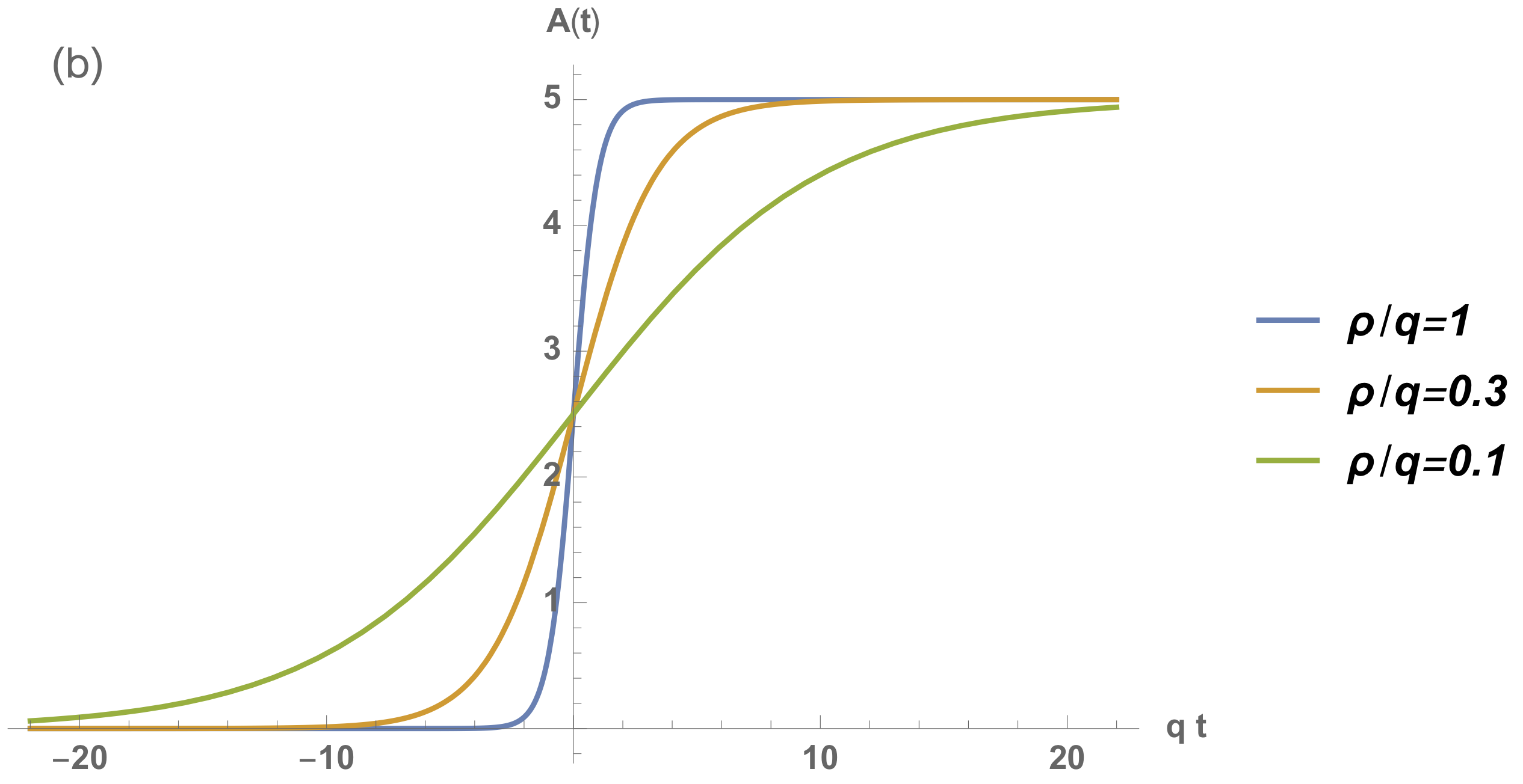 |
We have chosen the above Sauter-type pulse Sauter for convenience. Note that this potential is bounded both at early and late times (see Fig.2). Note also that for all the figures we work with dimensionless variables. The adiabatic limit is an extremely slow evolution of the potential, obtained when . We have to remark that the adiabatic limit is not the limit of a vanishing electric field. If the electric field had support in a bounded period of time, there would not be production of particles when . But the adiabatic limit is a more subtle limit, in which the electric field varies very slowly. Although when , the width of the pulse is also very large maintaining constant and non-vanishing the integral
| (13) |
To clarify things we remark that a different scenario is given by the alternative choice , with a constant value, independent of . The limit corresponds then to a constant electric field, with an unbounded potential . This produces, as expected, the Schwinger-type rate of pair creation by a constant electric field FN. In this paper we focus our analysis in the adiabatic limit in (11) and (12), as it produces a bounded potential and a completely analogous situation to that considered in the cosmological scenario. As we will show later on, in this case, it is indeed possible to produce particles by the electric field if extra conditions are met (i.e., a massless field, or the presence of magnetic fields in the four-dimensional case with fermions).
Inserting the potential (12) in (10) we obtain the physical solution in terms of the usual hypergeometric functions
| (14) |
where , , and . We have fixed this solution by demanding that at early times the modes behave as the Minkowskian modes for a free scalar field
| (15) |
At late times the modes behave as
| (16) |
where and are the Bogoliubov coefficients. They satisfy the relation according to the normalization condition (9). These coefficients serve to relate the early time creation and annihilation operators , defining the initial Fock space, with the late time operators
| (17) | |||
| (18) |
Therefore, we can define the number operator as
| (19) |
where is the number density of quanta (i.e., particles and antiparticles). Taking the late time limit in (14) and matching with (16) we obtain
| (20) | |||
| (21) |
where we have used the usual properties of the hypergeometric function mathbook. Finally we get
| (22) |
Fig. 3 shows a representation of this expression for different values of and , which can be interpreted as the momentum distribution of the created particles (the spectra of antiparticles would be obtained by making the shift ). We easily observe that decreases as , for fixed . In the same way, the particle density also decreases for large with fixed. Note in passing that for a sudden electric pulse () the momentum distribution of the particles is concentrated in the characteristic values and .

 |
To see whether vanishes in the adiabatic limit we analyze in detail the behavior on (22). We get
| (23) |
where and . Since , the first two terms vanish as . For , the function has a minimum at , with a value . It means that , and hence when , as in the case of a gravitational field. According with that, in Fig. 3(a) one can realize how the number of particles decreases with the adiabatic parameter , vanishing in the limit . However, for this is no longer valid since for , and hence , meaning that particles are being produced even in the adiabatic limit. In short, we have obtained, when ,
In order to visualize this behavior, we represent in Fig. 4 the dependence of the total density of created particles (given by (19)) on the parameter . One can see how in the adiabatic limit the density of quanta tends to vanish, except in the case , for which it tends to a non-zero value. This value is given by
| (27) |
This implies that the particle number is not an adiabatic invariant for the massless case. Furthermore, as we will see in the next section, the above result for the density number of created particles in the adiabatic limit coincides exactly with the analogous result for massless Dirac particles.

For completeness we will study now the vacuum expectation values of the electric current and the energy density induced by the underlying particle creation process. This will also serve to test the adiabatic invariance, or the breaking of it, in terms of the current and the energy density.
III.1 Electric current
For a two-dimensional charged scalar field, the electric current is given by . The vacuum expectation of this observable is UV-divergent and has to be renormalized. In the context of an homogeneous and time dependent background it is very convenient to use the adiabatic regularization/renormalization method described in FNP; FN. After performing the appropriated subtractions, one obtains
| (28) |
where are the mode functions of the scalar field satisfying the equation of motion (10) and . For more details on the original adiabatic method for scalar fields see parker-fulling.
Let us focus on the late-time behavior of the electric current, for which we can relate (28) to the Bogoliubov coefficients computed in the last section. We restrict again the analysis to an electric-pulse configuration (12) with bounded asymptotic states. Introducing (16) in (28) we have
| (29) |
It is easy to see that the terms which are independent of the Bogoliubov coefficients do not contribute to the electric current. One can derive this result by realizing that the first two terms correspond to linearly divergent integrals, differing by a constant shift
| (30) |
while the last term in (29) is a finite integral, which cancels with (30). The second term in (29) depends on time and produces oscillations of the form . In the limit the Riemann-Lebesgue lemma ensures that the integral in of this term vanishes. With the above considerations, and using the symmetry properties of (reflection under ), one can rewrite the expression of the electric current as follows:
| (31) |
This equation shows explicitly the close relation between the density of created quanta and the electric current. The first term accounts for particles and the second one for antiparticles. In the adiabatic limit, and for massive particles, the renormalized electric current also vanishes since . However, the last result changes completely if . As we have shown, in the adiabatic limit for . Therefore, the current at late times for massless particles in the adiabatic limit is given by
| (32) |
As expected, a non vanishing particle number , even in the adiabatic limit, induces an electric current different from zero.
III.2 Energy density
The renormalized vacuum expectation value of the energy density of a two-dimensional scalar field interacting with an electric field is given by
| (33) |
where are again the mode functions of the scalar field and the three last terms account for the adiabatic subtractions required by renormalization FNP. As for the electric current, we will we focus on the late time behavior. Plugging (16) in (33) and using the asymptotic expansion for the functions
| (34) |
we finally obtain
| (35) |
Using the same arguments as in section III.1, it is easy to see that the only term contributing to the energy density is the one proportional to . After some simplifications, we get the relation between the energy density and the particle number
| (36) |
where . In the adiabatic limit, we get , and therefore . Nevertheless, for there is indeed creation of energy. As we said, the adiabatic limit for the massless case gives us a non vanishing for . In this region, , and therefore the created energy density is
| (37) |
IV Breaking of adiabatic invariance in fermionic pair production by electric fields in two dimensions
Let us consider now a two-dimensional charged Dirac field interacting with an homogeneous, time-dependent electric field. The corresponding Dirac equation is
| (38) |
where are the Dirac matrices satisfying the anticommutation relations and . [We follow here the convention that the electric charge of the fermion is ]. The electromagnetic field is assumed to be an external classical field, while is a quantized field interacting with the classical electric background. Assuming also that the electric field is described by the potential in the appropriate gauge, the Dirac equation (38) becomes
| (39) |
From now on we will use the Weyl representation (with )
We expand the field in momentum modes
| (47) |
where the two independent and normalized spinor solutions are
and are the creation and annihilation operators which fulfill the usual anti-commutation relations. The field equation (39) is converted into
| (54) | |||
| (55) |
and we have assumed the normalization condition . Let us consider, as in the scalar case, the electric pulse . With this input the mode equations (54) and (55) can be solved exactly in terms of hypergeometric functions
| (56) |
| (57) |
where , and . We have fixed the initial condition in order to recover the positive frequency solution for a free field at early times
| (58) |
At late times the modes can be written as
| (59) |
and are the Bogoliubov coefficients satisfying the relation . These coefficients relate the early time creation and annihilation operators with the late time operators as follows
| (60) | |||||
| (61) |
The density of created quanta is given by , where and . Therefore, the particle number is also
| (62) |
The matching of (56-57) with (59) at late times determines the Bogoliubov coefficients. For the beta coefficients we get
| (63) |
And after simplifying, we obtain
| (64) |
Some representations of this expression are shown in Fig.5. As in the scalar case, the number of particles decreases as and increases as . For fermions, the relation implies that for any value of , according to Pauli’s exclusion principle.

 |
In the massless case, irrespective of the value of , one obtains (see Fig. 5(b))
| (65) |
for , and hence
The total density of created quanta is
| (69) |
Note that the same result is obtained by performing the adiabatic limit in the scalar case. In contrast, this result is valid for any value of , which means that the number of created massless fermions does not depend on the history of , but only on its final value.
This non-vanishing result of the particle number implies again the breaking of the adiabatic invariance.
For massive fermions and in the limit , expression (64) behaves essentially as
| (70) |
where . For , the former has a minimum at , with a value . Hence, and , as we can see in Fig. 5(a). Therefore we can conclude that the particle number is an adiabatic invariant for massive fermions, as in the scalar case. To visualize this behavior, we have depicted in Fig. 6 the dependence of the total density of created particles on the parameter . We can also observe that the density of quanta in the massless case does not vanish and, in contrast to the scalar case, it remains constant, according to the above calculations.

IV.1 Electric current
Using the renormalization method described in FN; BFNV; BNP for a Dirac field interacting with an homogeneous time-dependent electric field, the vacuum expectation value of the electric current is given by
| (71) |
To study the explicit dependence of the electric current with the mass, we can compute their time derivative
| (72) |
It is immediate to see that in the massless limit the first term vanishes, and the equation below can be easily integrated. With as initial condition one obtains
| (73) |
Note again that at each instant , the value of the electric current depends only on the value of the potential vector at , and not on its history.
This contrasts with the behavior of the created current for a massive field, since and depend on the particular shape of the electric pulse. In the latter case, and assuming the electric pulse configuration given in (12), it can be proven by using the Bogoliubov coefficient (64) and repeating the same calculations done in Section IIIA, that the electric current vanishes in the adiabatic limit. The analysis of the renormalized energy density can be carried out analogously, and it leads to a similar physical conclusion.
As a final comment, and for completeness, we remark that in the massless case, one can directly solve the semiclassical Maxwell equations for the electric field . Assuming, for instance, the initial conditions and the previous equation can be easily integrated, with solution . We find harmonic oscillations with frequency . This is consistent with the well-known fact that radiative corrections to the Schwinger model induce a mass for the “photon”, with a value Schwinger62; qftbook.
IV.2 Relation with the axial anomaly
We have found that the expected adiabatic invariance of the particle number observable fails for a massless Dirac field. This is accompanied with a non-vanishing electric current, even in the adiabatic limit, as can be read from (73). Furthermore, this result brings about a creation of chirality as a consequence of the fact that, in two-dimensions, the axial current is related by duality to the electric current . Hence, the result (73) implies the axial anomaly Bertlmann
| (74) |
In fact, one can also interpret the breaking of the adiabatic invariance as a natural and necessary consequence required by the axial anomaly. We remark that the loss of the adiabatic invariance of the particle number for a scalar field in two-dimensions, which coincides quantitatively with the result for fermions, can also be naturally interpreted in the language of anomalies. In two-dimensions, a massless scalar field inherits a classical chiral-type symmetry, in the sense that the classical wave equation splits into two disconnected sectors: right and left-moving degrees of freedom, as the fermionic two-dimensional field. The corresponding right and left electric currents are, in the adiabatic limit, separately conserved in the classical theory. However, in the quantum theory these currents also cease to be conserved. The creation of right and left electric currents in the quantum theory is exactly the same for massless scalar and Dirac fields in the adiabatic limit, as can be easily observed from (73) and (32).
V Generalization of previous results to 4D
In the previous sections we have shown that the particle number operator is not an adiabatic invariant for two-dimensional massless fields. Here, we extend our analysis to four dimensions for both scalar and fermionic fields. We briefly study whether the breaking of the adiabatic invariance could also happen in electric and magnetic backgrounds.
V.1 Scalar field
Consider now a charged scalar field obeying the wave equation , where we assume an homogeneous electric pulse defined by the vector potential with given again by (12). The Fourier expansion of the quantized field is
| (75) |
The mode functions satisfy the normalization condition and their time evolution is given by
| (76) |
This equation is very similar to the one found in the two-dimensional case (10). It allows us to partially reduce the four-dimensional problem to a two-dimensional one, by introducing an effective mass . Therefore, the beta coefficients can be obtained from Eq. (22) replacing by and by .
According to our previous results for scalar fields, only for and one can have a non-vanishing in the adiabatic limit. However, since and are continuous quantum numbers characterizing the modes, the amount of created particles is diluted into the infinite-volume of the unbounded three-dimensional space. Therefore, the total number density of produced particles turns out to be an adiabatic invariant.
This result cannot be altered by the introduction of a magnetic field. Adding a constant magnetic field in the -direction and choosing , the Fourier expansion for the scalar field is
| (77) | |||||
where
| (78) |
, and are the Hermite polynomials with . For simplicity, and without loss of generality, we have assumed . The time evolution is given by
| (79) |
From the two-dimensional viewpoint, the effective value of the mass, given now by , is a positive quantity, even for and . Using again the result of Section III we can similarly conclude that the particle number, defined now as
| (80) |
is also an adiabatic invariant for a scalar field in four dimensions, regardless of the value of the mass, given that . This is in sharp contrast with the result obtained for a massless scalar field in two dimensions. Note that for a scalar field in four dimensions there is no analog of the axial anomaly.
V.2 Dirac field
We can repeat the analysis for Dirac fermions. For massive fermions adiabatic invariance is preserved. Therefore we will focus on the massless case. In the latter, one can split the Dirac spinor in two independent chiral parts . For the left sector the Weyl equation reads . Considering an homogeneous electric pulse with vector potential given by (12), the Fourier expansion of the quantized field is
| (81) |
The two independent and normalized spinor solutions can be expressed as:
where . The equations for the modes are
| (88) | |||
These equations are similar to the ones found in the two-dimensional case (54) and (55), with an effective mass . Hence, the beta coefficients are given by Eq. (64) with the obvious replacements. As in the scalar case, only for one can have a non-vanishing beta coefficient in the adiabatic limit, therefore the amount of created particles is diluted and the total number density of produced particles is an adiabatic invariant. However, this is no longer true in the presence of a magnetic field. Adding a constant magnetic field in the -direction and choosing , the generic form of the modes for a massless field is
where is defined as in the scalar case (78). The time evolution of the modes is given by
| (95) | |||
In this case, we can identify the effective mass as , which vanishes at . Therefore, in the adiabatic limit, the beta coefficients (we recall they can also be obtained from the two-dimensional analog (64)) vanish for any value of except for . Since , the particle number tends to a non-zero value because the discrete state survives after summation. This contrasts with the previous case in which the mode was diluted after integration. Hence, the particle number is no longer adiabatic invariant.
This result is also linked to the axial anomaly, as happens in two dimensions. Note that in four dimensions the anomaly is only non-zero when both electric and magnetic fields are present. As in the two-dimensional case, the adiabatic anomaly must be reflected in the electric current and also in the chiral charge density . Repeating the previous analysis for the right part and computing the formal vacuum expectation value one finds
| (96) |
From this result one can easily see the special role of the modes, which are the only ones contributing to the breaking of the adiabatic invariance. Although in the most general case all the modes contribute to the electric current, in the adiabatic limit the contribution of the modes with , for which , will vanish, as happens in the two-dimensional case. This gives us a lower bound for the current. On the other hand, by looking at the chiral charge
| (97) |
one realizes that only the mode with creates chirality, even in a non-adiabatic regime. Furthermore, it is immediate to see that the lower bound of the electric current is given by .
VI Conclusions
We have reexamined the adiabatic invariance of the particle number operator of quantized fields in two dimensions coupled to a background electric field with bounded vector potential. We have pointed out that, for massless fields, the expected adiabatic invariance fails. This fact is accompanied by the emergence of the axial anomaly in two dimensions. In other words, the breaking of the adiabatic invariance (pair creation even in the limit ) is required to keep physical consistency with the axial anomaly. We have also shown that the breaking of the adiabatic invariance is also reproduced for a massless Dirac field in four dimensions, but requiring the presence of electric and magnetic fields, showing up again a deep connection with the axial anomaly.
Acknowledgments.– We thank I. Agullo and A. del Rio for very useful discussions. This work was supported by Grants. No. FIS2017-84440-C2-1-P, No. FIS2017-91161-EXP, No. SEJI/2017/042 (Generalitat Valenciana), No. SEV-2014-0398. P. B. is supported by a Ph.D. fellowship, Grant No. FPU17/03712. S. P. is supported by a Ph.D. fellowship, Grant No. FPU16/05287. A. F. is supported by the Severo Ochoa Ph.D. fellowship, Grant No. SEV-2014-0398-16-1, and the European Social Fund.
References
- (1) L. Parker, The creation of particles in an expanding universe, Ph.D. thesis, Harvard University (1966). Dissexpress.umi.com, Publication Number 7331244; Phys. Rev. Lett. 21, 562 (1968); Phys. Rev. D 183, 1057 (1969); Phys. Rev. D 3, 346 (1971).
- (2) L. Parker and D. J. Toms, Quantum Field Theory in Curved Spacetime: Quantized Fields and Gravity, Cambridge University Press, Cambridge, England (2009).
- (3) N. D. Birrell and P. C. W. Davies, Quantum Fields in Curved Space, Cambridge University Press, Cambridge, England (1982).
- (4) L. Parker, J. Phys. A 45, 374023 (2012).
- (5) W. Pittrich and H. Gies, Probing the Quantum Vacuum, Springer, Heidelberg (2000).
- (6) The extreme light infrastructure (ELI) project: www.extreme-light-infrastructure.eu/
- (7) J. Schwinger, Phys. Rev. 82, 664 (1951).
- (8) L. A. Kofman, A. D. Lindle, and A. A. Starobinsky, Phys. Rev. Lett. 73, 3195 (1994); Phys. Rev. Lett. 76, 1011 (1996).
- (9) N. Mueller, F. Hebenstreit, and J. Berges Phys. Rev. Lett. 117, 061601 (2016); S. P. Kim and H. K. Lee Phys. Rev. D 76, 125002 (2007).
- (10) G. V. Dunne, Int. J. Mod. Phys. A 27, 1260004 (2012); Eur. Phys. J. D 55, 327 (2009); B. S. Xie, Z. L. Lie, and S. Tang, Matter Radiat. Extremes, 2, 225 (2017).
- (11) R. Ruffini, G. Vereshchagin and S. Xue, Phys. Rep. 487, 1 (2010).
- (12) M.E. Peskin and D. V. Schroeder, An Introduction to Quantum Field Theory, Addison-Wesley, Reading, MA, USA (1995).
- (13) W. Israel, Phys. Rev. Lett. 57, 397 (1986).
- (14) S. W. Hawking, Black Holes aren’t Black, Gravity Research Foundation (1974), essay [www.gravityresearchfoundation 738 .org/year#1974]; Commun. Math. Phys. 43, 199 (1975).
- (15) A. Fabbri and J. Navarro-Salas, Modeling Black Hole Evaporation, ICP-World Scientific, London (2005).
- (16) F. Sauter, Z. Phys. 69, 742 (1931).
- (17) A. Ferreiro and J. Navarro-Salas, Phys. Rev. D 97, 125012 (2018).
- (18) M. Abramowitz, and I. A. Stegun, Handbook of Mathematical Functions: With Formulas, Graphs and Mathematical Tables, Dover, New York (1972).
- (19) A. Ferreiro, J. Navarro-Salas and S. Pla, Phys. Rev. D 98, 045015 (2018).
- (20) L. Parker and S. A. Fulling, Phys. Rev. D 9, 341 (1974); S. A. Fulling and L. Parker, Ann. Phys. (N.Y.) 87, 176 (1974); P. R. Anderson and L. Parker, Phys. Rev. D 36, 2963 (1987); I. Agullo, J. Navarro-Salas, G. J. Olmo and L. Parker, Phys. Rev. Lett. 103, 061301 (2009); Phys. Rev. D 81, 043514, (2010); A. Landete, J. Navarro-Salas and F. Torrenti, Phys. Rev. D 89 044030 (2014); S. Ghosh, Phys. Rev. D 91, 124075 (2015); I. Agullo, W. Nelson and A. Ashtekar Phys. Rev. D 91, 064051 (2015); A. del Rio and J. Navarro-Salas, Phys. Rev. D 91, 064031 (2015); S. Ghosh, Eur. Phys. J. C 79, 239 (2019); A. Ferreiro and J. Navarro-Salas, Phys. Lett. B 792, 81 (2019).
- (21) J. F. Barbero G., A. Ferreiro, J. Navarro-Salas and E. J. S. Villaseñor, Phys. Rev. D 98, 025016 (2018).
- (22) P. Beltrán-Palau, J. Navarro-Salas and S. Pla, Phys. Rev. D 99 105008 (2019).
- (23) J. Schwinger, Phys. Rev. 128, 2425 (1962).
- (24) R. A. Bertlmann, Anomalies in Quantum Field Theory, Oxford University Press, Oxford (2000).