Side Window Filtering

Hui Yin Thanks: authors equally contribute to this paper Affiliation: College of Information Engineering and Guangdong Key Lab for Intelligent Information Processing, Yuanhao Gong Guoping Qiu Affiliation: College of Information Engineering and Guangdong Key Lab for Intelligent Information Processing, Shenzhen University China School of Computer Science The University of Nottingham UKyinhui0606@gmail.com gong@szu.edu.cn guoping.qiu@nottingham.ac.uk

Abstract

Local windows are routinely used in computer vision and almost without exception the center of the window is aligned with the pixels being processed. We show that this conventional wisdom is not universally applicable. When a pixel is on an edge, placing the center of the window on the pixel is one of the fundamental reasons that cause many filtering algorithms to blur the edges. Based on this insight, we propose a new Side Window Filtering (SWF) technique which aligns the window’s side or corner with the pixel being processed. The SWF technique is surprisingly simple yet theoretically rooted and very effective in practice. We show that many traditional linear and nonlinear filters can be easily implemented under the SWF framework. Extensive analysis and experiments show that implementing the SWF principle can significantly improve their edge preserving capabilities and achieve state of the art performances in applications such as image smoothing, denoising, enhancement, structure-preserving texture-removing, mutual-structure extraction, and HDR tone mapping. In addition to image filtering, we further show that the SWF principle can be extended to other applications involving the use of a local window. Using colorization by optimization as an example, we demonstrate that implementing the SWF principle can effectively prevent artifacts such as color leakage associated with the conventional implementation. Given the ubiquity of window based operations in computer vision, the new SWF technique is likely to benefit many more applications.

1 Introduction

(a) Step Edge

(b) Ramp Edge

Figure 1: Model of ideal edges in 2D piecewise images. The pixel ‘a’

\sim

‘f’ are on edges or near edges. To satisfy the linear assumption, they should be approximated in the side windows which have the same colors with them, not the local windows centered at them.

In the fields of computational photography and image processing, many applications involve the concept of image filtering to denoise denoise, deblur deblur and enhance details details. For decades, various filters have been developed, such as box filter, Gaussian filter and median filter, to name a few. These filters are widely used in image deblurring and sharpening, edge detection and feature extraction book1.

There are many applications require image filtering that can preserve edges. Typical examples include tone mapping of high dynamic range (HDR) images hdr, detail enhancement via multi-lighting images enhancement, and structure-preserving and texture removing rtvrgf.

For this reason, many edge-preserving filters have been proposed. Basically, these edge-preserving filters can be divided into two categories. One is global optimization based algorithms, such as the total variation (TV) algorithm denoise, its iterative shrinkage approach tv1, the relative total variation algorithm rtv and the weighted least squares algorithm wls. The other is local optimization based algorithms, such as bilateral filter bf, its accelerated versions fbffbf1fbf2, guided filter gf, its extensions wgfggf, rolling guidance filter rgf, mutual structure joint filtering msfjf and curvature filter details. In general, the local based filters can be calculated in real time. This is preferred because many real application scenarios require real-time processing.

1.1 Filtering Fundamentals

Local based filters always attempt to estimate an output of a pixel based on its neighbors. Almost without exception, the pixel being processed is located at the center of an operation window and other pixels in the operation window are its neighbors. Basically, there are two ways to do estimation: linear approximation, such as box filter and Gaussian filter, and non-linear approximation, such as median filter mf, bilateral filter bf and guided filter gf.

A common linear approximation based image filtering operation assumes that the image is piecewise linear and approximate a pixel as the weighted average of its neighbor pixels over a local window

I_{i}^{{}^{\prime}}=\sum_{j\in\Omega_{i}}{\omega_{ij}q_{j}}

(1)

where $\Omega_{i}$ is the local window (support region) centered at the pixel $i$ , $\omega_{ij}$ denotes the weight kernel, $q_{i}$ and $I_{i}$ are the intensities of the input image $q$ and the output image $I$ at location $i$ , respectively.

The discrepancy between the filter output and the original image can be formulated as the following cost function

E_{i}=||I_{i}-I_{i}^{{}^{\prime}}||_{2}^{2}=(I_{i}-\sum_{j\in\Omega_{i}}{\omega_{ij}q_{j}})^{2}

(2)

Different weight kernels will result in different filtering output images and in most cases the task of designing a filtering algorithm is that of estimating the weights. Often there is a trade off between manipulating the input image towards a desired target and keeping it close to the original. It is worth noting that optimization problem of the form similar to eq. (2) is found in many applications including colorization colorizationcolorizationofqiu and image segmentation seg1seg2, where the weight functions are usually referred to as affinity functions. Nonlinear approximation filtering such as median filtering can also be formulated as a similar form of optimization problem med1.

1.2 Problem and Motivation

In many applications that using the form of filtering algorithm in eq. (1), it is desired to smooth out genuine noise and at the same time preserve edges and other signal details. For analysis convenience, we focus our study on three types of typical edges cie, step edge, ramp edge and roof edge, and model them in 2D signal space as shown in Fig. 1. We use $g(x,y)$ to denote the intensity value at $(x,y)$ . The functions $g(x,y)$ shown in this figure are continuous but non-differentiable. Considering the locations where the intensity changes (an edge), for example, at location ‘a’. We use ‘a-’ and ‘a+’ to denote the left limit ( $x-\epsilon,y$ ) and right limit ( $x+\epsilon,y$ ), respectively, where $\epsilon>0$ . Clearly, $g(x-\epsilon,y)\neq g(x+\epsilon,y)$ and (or) $g^{\prime}(x-\epsilon,y)\neq g^{\prime}(x+\epsilon,y)$ due to the edge jump. Therefore, the Taylor expansion at these two regions are different: $g(x-2\epsilon,y)\approx g(x-\epsilon,y)+g^{\prime}(x-\epsilon,y)(-\epsilon)$ and $g(x+2\epsilon,y)\approx g(x+\epsilon,y)+g^{\prime}(x+\epsilon,y)\epsilon$ . Therefore, any approximation at location ‘a-’ must come from the left regions of ‘a’ while any approximation at location ‘a+’ must come from the right regions of ‘a’. Similar statements apply for other edge locations such as ‘b’, ‘c’, and ‘d’ in Fig. 1.

Based on the analysis and eq. (1), if a pixel $i$ is on an edge, the support region $\Omega_{i}$ must be restricted to one side of the edge, otherwise, it is not possible to use a linear combination of the neighbors to approximate $i$ . In other words, we cannot place the center of $\Omega_{i}$ over $i$ but rather we must place the side of $\Omega_{i}$ over $i$ . Inspired by this discovery, a new edge-preserving strategy, termed side window filtering (SWF) technique, is proposed. We consider each target pixel as a potential edge and generate multiple local windows (named as side windows) around it, each of which aligns the target pixel with a side or a corner (instead of the center) of the window. The output of SWF is a linear combination of the neighbors in one of the side windows which can best approximate the target pixel.

1.3 Our Contributions

The novel contributions of this paper are:

1. Using Taylor expansion, we show that in order to reconstruct an edge pixel using a linear combination of its neighbors, the neighbor pixels must come from one side of the edge. Based on this insight, we propose the side window filtering (SWF) technique as an effective and practical edge preserving filtering solution.

2. We show how traditional linear filters such as box filter and Gaussian filter, popular non-linear filters such as median filter, bilateral filter and guided filter can easily be implemented under the SWF framework. Through extensive analysis, we show that implementing these popular filters based on the new SWF framework can significantly improve their edge preserving capabilities.

3. We show that the implementing traditional filters under the new SWF framework provides state of the art performances in a variety of real world applications including image smoothing, denoising, enhancement, structure-preserving texture-removing, mutual-structure extraction, and high dynamic range image tone mapping.

4. We show that the new SWF framework can be extended to other applications involving a local window and a linear combination of a neighborhood of pixels. Using colorization by optimization as an example we demonstrate that implementing the SWF principle can effectively prevent artifacts such as color leakage.

5. The SWF technique is very simple but theoretically rooted and in practice surprisingly effective. Given the ubiquity of window based operations, the SWF principle has the potential of benefiting many areas in image processing and computer vision.

Figure 2: Definition of side window.

r

is the radius of the window. (a) The definition of side window in continuous case. (b) The

left

(red rectangle) and

right

(blue rectangle) side windows. (c) The

up

(red rectangle) and

down

(blue rectangle) side windows. (d) The

northwest

(red rectangle),

northeast

(blue rectangle),

southwest

(green rectangle) and

southeast

(orange rectangle) side windows.

2 Side Window Filtering Technique

First of all we define the side window in a continuous case. The definition of a side window is shown in Fig. 2(a), with parameters $\theta$ and $r$ . $\theta$ is the angle between the window and the horizontal line, $r$ is the radius of the window, $\rho\in\{0,r\}$ and $(x,y)$ is the position of the target pixel $i$ . $r$ is a user-defined parameter and it will be fixed for all the side windows. By changing $\theta$ and fixing $(x,y)$ , we can change the direction of the window while aligning its side with $i$ .

To simplify the calculation, we only define eight side windows in a discrete case, as shown in Fig. 2(b) $\sim$ (d). These eight specific windows correspond to $\theta=k\times\frac{\pi}{2},k\in[0,3]$ . By setting $\rho=r$ , we have the $down(D)$ , $right(R)$ , $up(U)$ , $left(L)$ side windows, denoted as $\omega^{D}_{i}$ , $\omega^{R}_{i}$ , $\omega^{U}_{i}$ and $\omega^{L}_{i}$ . They align $i$ with their sides. By setting $\rho=0$ , we have the southwest ( $SW$ ), southeast ( $SE$ ), northeast ( $NE$ ) and northwest ( $NW$ ) side windows, as shown in Fig. 2(d) and denoted as $\omega^{SW}_{i}$ , $\omega^{SE}_{i}$ , $\omega^{NE}_{i}$ and $\omega^{NW}_{i}$ . They align $i$ with their corners. It is worth pointing out that there is significant flexibility in designing the size, shape and orientation of the side windows. And the only specific requirement is that the pixel under consideration is placed on the side or corner of the window.

Algorithm 1 Calculate the SWF for each pixel

w_{ij}

is the weight of pixel

j

, which is in the neighborhood of the target pixel

i

, based on kernel function

F

S=\{L,R,U,D,NW,NE,SW,SE\}

is the set of side window index.

I_{\mathrm{{n}}}=\frac{1}{N_{\mathrm{{n}}}}\mathop{\sum}_{j\in\omega^{\mathrm{{n}}}_{i}}w_{ij}q_{j}

N_{\mathrm{{n}}}=\mathop{\sum}_{j\in\omega^{\mathrm{{n}}}_{i}}w_{ij},\mathrm{{n}}\in S

2: find

I_{m}

, such that

I_{m}=\mathop{\operatorname*{argmin}_{n\in S}{||q_{i}-I_{n}||_{2}^{2}}}

I_{m}

By applying a filtering kernel $F$ in each side window, we can obtain eight outputs, denoted as $I_{i}^{{}^{\prime}\theta,\rho}$ , where $\theta=k\times\frac{\pi}{2},k\in[0,3]$ and $\rho\in\{0,r\}$

I_{i}^{{}^{\prime}\theta,\rho,r}=F(q_{i},\theta,\rho,r)

(3)

To preserve the edges means that we want to minimize the distance between the input and the output at an edge, i.e., the filter output should be the same as or as close as possible to the input at an edge. Therefore, we choose the output of the side window that has the minimum $L_{2}$ distance to the input intensity as the final output,

I^{\prime}_{SWF}=\mathop{argmin}_{\forall I_{i}^{{}^{\prime}\theta,\rho,r}}||q_{i}-I_{i}^{{}^{\prime}\theta,\rho,r}||_{2}^{2}

(4)

where $I^{\prime}_{SWF}$ is the output of SWF. Eq. (4) is referred to as the SWF technique. Details of the procedure is described in Algorithm 1.

Table 1: Summary of the output of BOX and S-BOX

Input	BOX	S-BOX
(a)	$\frac{(r+1)u+rv}{2r+1}$	$u$
(d)	$\frac{(r+1)u+rv}{2r+1}$	$u$
(g)	$\frac{(r+1)u+rv}{2r+1}$	$u$
(j)	$\frac{(r+1)^{2}u+((2r+1)^{2}-(r+1)^{2})v}{(2r+1)^{2}}$	$u$
(m)	$u+\frac{r(r+1)\vartriangle{v}}{2(2r+1)}$	$u$
(p)	$v-\frac{r(r+1)\vartriangle{u}}{2r+1}$	$v-\frac{r}{2}\vartriangle{u}$

Figure 3: Comparing BOX and S-BOX on the testing images with different edges. The first and forth columns (a), (g), (m), (d), (j) and (p) are input images with edge or corner. The second and fifth columns are middle line profiles for input, BOX filter and S-BOX filter. The third and sixth columns are the zoomed in region at the edge or corner location.

Table 2: Summary of the output of each side window in S-BOX

Case	L	R	U	D	NW	NE	SW	SE
(a)	u	$\frac{u+rv}{r+1}$	$\frac{(r+1)u+rv}{2r+1}$	$\frac{(r+1)u+rv}{2r+1}$	u	$\frac{u+rv}{r+1}$	u	$\frac{u+rv}{r+1}$
(d)	$\frac{(r+1)u+rv}{2r+1}$	$\frac{(r+1)u+rv}{2r+1}$	u	$\frac{u+rv}{r+1}$	u	u	$\frac{u+rv}{r+1}$	$\frac{u+rv}{r+1}$
(g)	$\frac{(\frac{3r}{2}+1)u+\frac{r}{2}v}{2r+1}$	$\frac{(\frac{r}{2}+1)u+\frac{3r}{2}v}{2r+1}$	$\frac{(\frac{3r}{2}+1)u+\frac{r}{2}v}{2r+1}$	$\frac{(\frac{r}{2}+1)u+\frac{3r}{2}v}{2r+1}$	u	$\frac{(\frac{r}{2}+1)u+\frac{r}{2}v}{r+1}$	$\frac{(\frac{r}{2}+1)u+\frac{r}{2}v}{r+1}$	$\frac{((r+1)^{2}-1)v+u}{(r+1)^{2}}$
(j)	$\frac{(r+1)u+rv}{2r+1}$	$\frac{u+2rv}{2r+1}$	$\frac{(r+1)u+rv}{2r+1}$	$\frac{u+2rv}{2r+1}$	u	$\frac{u+rv}{r+1}$	$\frac{u+rv}{r+1}$	$\frac{((r+1)^{2}-1)v+u}{(r+1)^{2}}$
(m)	u	$u+\frac{r}{2}\vartriangle{v}$	$u+\frac{r(r+1)\vartriangle{v}}{2(2r+1)}$	$u+\frac{r(r+1)\vartriangle{v}}{2(2r+1)}$	u	$\frac{u}{r+1}+\frac{r}{2}\vartriangle{v}$	u	$\frac{u}{r+1}+\frac{r}{2}\vartriangle{v}$
(p)	$v-\frac{r}{2}\vartriangle{u}$	$v-\frac{r}{2}\vartriangle{u}$	$v-\frac{r(r+1)\vartriangle{u}}{2r+1}$	$v-\frac{r(r+1)\vartriangle{u}}{2r+1}$	$v-\frac{r}{2}\vartriangle{u}$	$v-\frac{r}{2}\vartriangle{u}$	$v-\frac{r}{2}\vartriangle{u}$	$v-\frac{r}{2}\vartriangle{u}$

2.1 Analysis of SWF

In this section, we present a detailed analysis of the edge-preserving property of SWF technique. For analysis convenience, we use box filter (BOX) as an example and similar analysis can be performed on other forms of filter. This means that $F$ in eq. (3) is averaging and the resulting filter is called side window box filter (S-BOX).

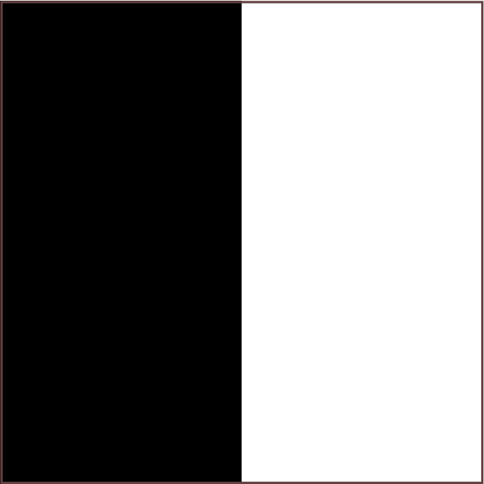
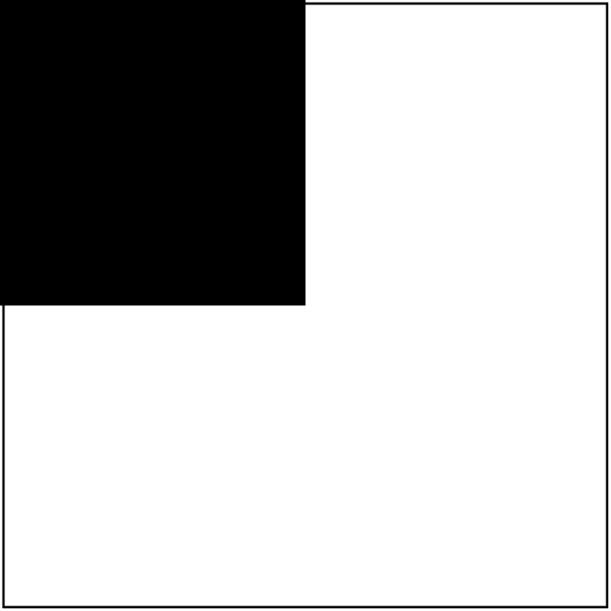
We compare the edge-preserving property of BOX and S-BOX filters. First of all, testing images with typical edges are generated, as shown in Fig. 3. There are six typical edges, including vertical edge (a), horizontal edge (d), diagonal edge (g), corner (j), ramp edge (m) and roof edge (p). For the vertical edge, horizontal edge, diagonal edge and corner, the pixel values for the black part of the edge is $u$ and the white part of the edge is $v$ . For the ramp edge, the pixel values are increased from $u$ to $v$ with a step of $\vartriangle{v}$ . For the roof edge, the top of the roof is $v$ and is decreased with a step of $\vartriangle{u}$ . Based on these conditions, the outputs of BOX and S-BOX are deduced and the results are shown in Table 1. From Table 1, we can easily see that S-BOX better preserves the edges in (a) $\sim$ (m) than BOX. It is also easy to prove $\frac{r}{2}<\frac{r(r+1)}{2r+1}$ , so S-BOX can better preserve the roof edge than BOX, too.

In order to observe the details of the edge-preserving property of each side window in S-BOX, the output of each side window is shown in Table 2. The results which preserve the edges are shown in bold. We can make the following observations:

•

the $L,NW,SW$ side windows can preserve the edges on the left of the vertical edge. It is easy to deduce that the $R,NE,SE$ side windows can preserve the edges on the right of the vertical edge.
•

the $U,NW,NE$ side windows can preserve the edges above the horizontal edge. Again, it is easy to deduce that the $D,SW,SE$ side windows can preserve the edges below the horizontal edge.
•

the $NW$ side window can preserve the edges above the diagonal edge and on the corner. It is easy to deduce that the $NE,SW,SE$ side windows can preserve the diagonal edges and corner with other directions.
•

the $L,NW,SW$ side windows can preserve the ramp edge.
•

although the side windows can not preserve the roof edge completely, seven of them have better results than BOX.

We also show the experimental results in Fig. 3. In the experiments, we set $u=0,v=1$ and $r=7$ . One line (or column or diagonal) of pixels is extracted from each result and zoomed in. The results are consistent with the theoretical deduction. Visually, the sharp edges are smoothed away by BOX while preserved very well by S-BOX.

3 Popular Filters under the SWF Framework

By changing $F$ to other kernels, one can easily embed the side window technique into other filters. In this section, we will discuss how to embed side window technique into Gaussian filter, median filter, bilateral filter and guided filter. To simplify expression, the filters’ name are abbreviated by their first three letters and their SWF versions are abbreviated by adding another ‘S-’. For example, the Gaussian filter and side window Gaussian filter are abbreviated as GAU and S-GAU, respectively.

In S-GAU, $F$ is a half of or a quarter of the Gaussian kernel. Because the kernel of GAU crosses over the potential edges, it may blur the edges. By contrast, the kernel of S-GAU alleviates this problem so it can better preserve the edges.

In S-MED, $F$ is the operation of calculating the median value. Since the output has the minimal distance from the input intensity, S-MED can better preserve the edges than MED. That is, it selects a window under which the median of the pixels is closest to the input.

In S-BIL, the kernel is calculated based on the geometric closeness and photometric similarity as in BIL. Since S-BIL can prevent the diffusion from crossing the edges, it can improve the edge-preserving property of BIL.

GUI averages the values of the parameters in all the windows that cover the target pixel. Again, this operation may blur potential edges. To avoid this problem, S-GUI ensures that the side windows do not cross over the target pixel. It slides each side window along its side on which the target pixel is located until the target pixel is outside of the side window. In this way, $2r+1$ sliding windows are obtained for the $L,R,U,D$ side window and averaged to obtain the outputs of these side windows. For the $NW,NE,SW,SE$ side windows, sliding can only get one output for each. The final output is chosen according to eq. (4).

4 Applications

In this section, the side window technique is applied to various image processing applications and its performance is compared with traditional filters and methods. More results are presented in the Supplement. The images are best viewed electronically on a high resolution monitor.

4.1 Image smoothing

Fig. 4 shows the smoothing results of the filters on an image ntire. The upper left part of each result is from the traditional filter and the zoomed in patch is with red rectangle. The lower right part of each result is from the side window version and the zoomed in patch is with green rectangle. As can be seen, the corresponding side window filter outperforms the original filter in preserving edges. This is more clearly shown in the zoomed in patches that the side window filters can better preserve the tiger’s whiskers. When comparing the non-linear filters, this improvement is also obvious. This means that the side window technique can also improve the edge-preserving property of non-linear filters. This shows the potential for the side window technique to be widely used in more applications.

4.2 Image denoising

Fig. 5 shows the results of iteratively applying different filters to remove noise of a low light image renoir. The left part of each result is from the traditional filter and the zoomed in patch is with red rectangle. The right part of each result is from the side window version and the zoomed in patch is with green rectangle. BOX, GAU, MED, BIL and GUI remove the noises but blur the edges at the same time. On the other hand, the side window version of these filters can preserve edges and remove noises at the same time. These results further demonstrate the excellent edge preserving property of the new side window technique.

4.3 Image enhancement

Image enhancement is often performed in image processing gfwgf. An enhanced image can be obtained by

Enhanced=q+\alpha\times(q-I^{{}^{\prime}})

(5)

where $\alpha$ is an amplification parameter and is fixed to 5 in all the experiments in this section. An example of image enhancement result is shown in Fig. 6. From the zoomed in patches, we can see that the halo artifacts exist along the edges in the results of the filters without implementing the side window technique. However, the artifacts have disappeared in the results of the side window versions of the filters. This can once again be attributed to the excellent edge-preserving property of the side window technique.

4.4 HDR tone mapping

In fbf a technique based on bilateral filter was proposed for displaying HDR images, which reduces the dynamic range while preserving detail. Briefly the operation works as follows:

I^{\prime}=\gamma\times q_{b}+q_{d}

(6)

$q_{b}$ is the bilateral filter output, $q_{d}$ is the difference between the original HDR radiance map and $q_{b}$ , and $\gamma\in(0,1)$ is the compression factor which determines the scale of dynamic range compression. For specific details please refer to fbf and their companion website eh3. In this experiment, we replace BIL and GUI by their side window versions.

Fig. 7 shows examples of the results. From the zoomed in patches, we can see that halo artifacts exist in the results of filters without side window technique, while they do not exist in the results of their side window filters. These results can once again be attributed to the good edge-preserving property of SWF.

4.5 Structure-preserving and texture-removing on natural image

The goal of this application is to extract image structures and remove the textures rtv. The side window technique is embedded into the weighted guided filter (WGF) wgf to form a new filter called S-WGF. By combining WGF and S-WGF in the iteration framework of rgf, we propose a new structure-preserving texture-removing filter, termed iterated side window weighted guided filter (IS-WGF). In this filter, an edge-aware weight wgf and a threshold $\lambda$ is used to easily distinguish structures from textures. The structures are preserved by S-WGF and textures are removed by WGF.

IS-WGF is compared with iterated weighted guided filter (IWGF), relative total variance (RTV) rtv and rolling guidance filter (RGF) rgf. IWGF is obtained by combining WGF with the iterative framework of rgf, RTV is the state of art of this application and RGF is the original algorithm in rgf. They are applied to smooth natural images with obvious textures and structures, as shown in Fig. 8(a). It is chosen from the BSR Dataset bsr. The wave in the sea is viewed as textures and the sailing boat on the sea is viewed as structures. From the results we can see that only IS-WGF can preserve the structures while all other filters fail. This example demonstrates the excellent structure-preserving property of side window technique.

4.6 Mutual structure extraction

In this section, the S-WGF is applied to the iteration framework of msfjf, which was proposed to extract structures co-existed in a reference image and a target image, to form a new filter termed Mutual-struture S-WGF (MS-WGF). The method in msfjf is referred to as MJF. We apply MJF and MS-WGF to extract the mutual structures of an RGB image and a depth image. The results are shown in Fig. 9. The results of MJF is obtained with 20 iterations (without post processing by median filter) and the results of MS-WGF is obtained with 10 iterations. These results demonstrate that with fewer iterations, MS-WGF performs as well as MJF. Moreover, the results on the depth image of MS-WGF is smoother than that of MJF and the non-mutual structures on the bear’s face are removed more thoroughly by MS-WGF.

4.7 Colorization

In addition to image filtering, our new side window technique can also be used to improve other local patch based algorithms, such as colorization by optimization colorization. The algorithm works in the $YUV$ color space. For a given intensity channel $Y(i)$ as input, the algorithm outputs two color channels $U(i)$ and $V(i)$ , where $i$ denotes a particular pixel, through optimizing the following cost function

J(U)=\mathop{\sum}_{i}\Big(U(i)-\sum_{j\in{N(i)}}\omega_{ij}U(j)\Big)^{2}

(7)

To implement the above colorization by optimization method in the SWF framework, we simply change the neighborhood $N(i)$ to a side window of $i$ (denoted to as $N_{s}(i)$ ) and keep all other aspects of the algorithm intact. Instead of a neighborhood centered on $i$ , we choose a suitable side window $N_{s}(i)$ that aligns its side or corner with $i$ . For each pixel, the best side window is chosen with a box filtering kernel (eq. 4).

Experiments have been carried out based on the image data and code provided in the web page of the authors of colorization. Some results are shown in Fig. 10. From the zoomed in patches, we can see that color leakage exists in the original method. But it is avoided when the original method is embedded with the side window technique. This is owing to the edge-preserving property of side window technique and demonstrating the wider applicability of the new side window technique.

5 Complexity Analysis

The order of complexity of side window based filters is the same as the original filters. However, as the SWF implementation needs to perform calculations over multiple windows, its computational cost is higher. Our experiments without code optimization are conducted on a computer with a 3.5GHz Intel core Xeon(R) CPU. For gray-scale images with 1 mega pixels, the computational time of the filters are shown in Table 3. The BIL is the original algorithm in bf without modification for acceleration. With code optimization and implementing GPU programming, the computational speed can be significantly improved. Our code will be made available publicly after the paper is published.

Table 3: The computational time on images with 1 mega pixels

Method	BOX	GAU	MED	BIL	GUI
Original	0.052	0.023	1.16	8.69	0.131
SWF version	0.215	0.23	3.67	26.2	0.431

6 Conclusion

Window based processing is one of the most common operations in computer vision. Traditional practices almost always align the center of the window with the pixel under processing. In this paper, we show that this widely used practice is not always the best solution. We show that in many applications, the side or the corner of the operation window instead of the center should be aligned with the pixel under processing and propose the side window filtering (SWF) technique. We have shown that many popular linear and non-linear filtering algorithms can be implemented based on this principle and the SWF implementation of these traditional filters can significantly boost their edge preserving capabilities. We have further shown that the SWF principle can be extended to other computer vision problems that involve a local operation window and a linear combination of the neighbors in this window such as colorization by optimization. We have shown that SWF technique can improve their performances and avoid artifacts such as color leakage that is often associated with such algorithm. Window based operations is extensively used in many areas of computer vision and machine learning including convolutional neural networks (CNNs). The SWF principle, i.e., aligning the edge or corner of the operation window with the pixel being processed, although seemingly trivial, is actually deeply rooted in the fundamental assumptions of many algorithms. Our theoretical analysis and state of the art results for many real world applications have demonstrated its effectiveness. We believe that there are many more applications can benefit from implementing the SWF principle.

References

(1) https://people.csail.mit.edu/fredo/publi/siggraph2002/.
(2) E. Agustsson and R. Timofte. Ntire 2017 challenge on single image super-resolution: Dataset and study. In The IEEE Conference on Computer Vision and Pattern Recognition (CVPR) Workshops, July 2017.
(3) J. Anaya and A. Barbu. Renoir - a dataset for real low-light image noise reduction. Journal of Visual Comm. and Image Rep, 51(2):144–154, 2018.
(4) H. Chidiac and D. Ziou. Classification of image edges. Vision Interface.
(5) F. Durand and J. Dorsey. Fast bilateral filtering for the display of high-dynamic-range images. ACM Trans. on Graphics, 21(3):257–266, 2002.
(6) Z. Farbman, R. Fattal, D. Lischinshi, and R. Szeliski. Edge-preserving decompositions for multi-scale tone and detail manipulation. ACM Trans. on Graphics, 27(3):67:1–67:10, 2008.
(7) R. Fattal, M. Agrawala, and S. Rusinkiewicz. Multiscale shape and detail enhancement for multi-light image collection. ACM Trans. on Graphics, 26(3):211–215, 2007.
(8) Y. Gong and I. Sbalzarini. A natural-scene gradient distribution prior and its application in light-microscopy image processing. IEEE Journal of Selected Topics in Signal Processing, 10(1):99–114, 2016.
(9) Y. Gong and I. Sbalzarini. Curvature filters efficiently reduce certain variational energies. IEEE Trans. Image Process, 26(4):1786–1798, 2017.
(10) R. Gonzalez and R. Woods. Digital image processing.
(11) K. He, J. Sun, and X. Tang. Guied image filtering. IEEE Trans. On Pattern Analysis and Machine Learning, 35(6):1397–1409, 2013.
(12) T. Huang, G. Yang, and G. Tang. A fast two-dimensional median filtering algorithm. IEEE Transactions on Acoustics, Speech and Signal Processing.
(13) F. Kou, W. Chen, C. Wen, and Z. Li. Gradient domain guided image filtering. IEEE Trans. Image Process, 24(11):4528–4539, 2015.
(14) A. Levin, D. Lischinski, and Y. Weiss. Colorization using optimization. ACM Trans on Graphics, 23(3):689–694, 2004.
(15) Z. Li, J. Zheng, Z. Zhu, W. Yao, and S. Wu. Weighted guided image filtering. IEEE Trans. Image Process, 24(1):120–129, 2015.
(16) D. Martin, C. Fowlkes, D. Tal, and J. Malik. A database of human segmentation algorithms and its application to evaluating segmentation algorithms and measuring ecological statistics. Proc. 8th Int’l Conf. Computer Vision, 2.
(17) O. Michailovich. An iterative shrinkage approach to total-variation image restoration. IEEE Trans. Image Process, 20(5):1281–1299, 2011.
(18) D. Min, S. Choi, J. Lu, B. Ham, K. Sohn, and M. Do. Fast global image smoothing based on weighted least squares. IEEE Trans. Image Process, 23(12):5638–5653, 2014.
(19) S. Paris and F. Durand. A fast approximation of the bilateral filter using a signal processing approach. ECCV.
(20) F. Porikli. Constant time o(1) bilateral filtering. CVPR.
(21) G. Qiu. Functional optimization properties of median filtering. IEEE Signal Processing Letters, 1(4):64–65, 1994.
(22) G. Qiu and J. Guan. Color by linear neighborhood embedding. IEEE International Conference on Image Processing.
(23) L. Rudin, S. Osher, and E. Fatemi. Nonlinear total variation based noise removal algorithms. Physica D, 60.
(24) X. Shen, C. Zhou, L. Xu, and J. Jia. Mutual-structure for joint filtering. IEEE International Journal of Computer Vision, 125.
(25) J. Shi and J. Malik. Normalized cuts and image segmentation. IEEE Transactions on Pattern Analysis and Machine Intelligence, 22(8):888–905, 2000.
(26) C. Tomasi and R. Manduchi. Bilateral filtering for gray and color images. ICCV.
(27) Z. Wang, A. Bovik, and H. Sheikh. Image quality assessment: from error visibility to structural similarity. IEEE Trans. on Image Processing, 13(4):600–612, 2004.
(28) Y. Weiss. Segmentation using eigenvectors: A unifying view. ICCV.
(29) L. Xu, Q. Yan, Y. Xia, and J. Jia. Structure extraction from texture via relative total variation. ACM Trans. on Graphics, 31(6):139:1–139:10, 2012.
(30) Q. Zhang, X. Shen, L. Xu, and J. Jia. Rolling guidance filter. ECCV.