Buffer-aided Resource Allocation for a Price Based Opportunistic Cognitive Radio Network
Abstract
In this paper, a resource allocation problem for an opportunistic cooperative cognitive radio network is considered, where cognitive radio nodes send their hard decisions to the fusion center. The fusion center plays dual role, i.e., takes the global decision (i.e., decision about the primary user’s activity) as well as allocates transmission time durations among cognitive radio nodes. Revenue based utility functions are considered at the fusion center and cognitive radio nodes. An optimization problem is formulated to maximize the fusion center’s revenue while satisfying some well defined constraints. User selection among cognitive radio nodes is performed in order to make the optimization problem feasible.
Index Terms:
Cognitive radio, spectrum sensing, resource allocation, user selectionI Introduction
In last few years, the communication industry has witnessed massive growth in number of wireless devices as well as traffic. As per the report by Cisco [1], number of global wireless users will rise to 5.5 billion in 2020 from 4.8 billion in 2015. The concept of spectrum sharing has emerged to cope with this ever increasing wireless data demand. In literature [2, 3, 4, 5, 6, 7], we find the usage of spectrum sharing concept in various forms like long term evolution-unlicensed (LTE-U), LTE-licensed assisted access (LTE-LAA), MULTEFIRE, licensed shared access (LSA), and spectrum access system (SAS). Spectrum sharing is considered one of the major requirements in 5G in order to make devices backward compatible [8, 9].
Cognitive radio (CR) [10] is considered as an efficient spectrum sharing technology, whose application can be found in different modern wireless communications contexts like machine-to-machine (M2M) [11], internet-of-things (IoT) [12], network virtualization [13], and hotspots [14]. For more information about past standardizations and current initiatives on CR technology in spectrum sharing, one may refer to [15] and [16] respectively. In CR networks, unlicensed secondary users (SUs) try to opportunistically access the primary user’s (PU’s) licensed spectrum with the help of spectrum sensing. In [17], we find different spectrum sensing techniques related to individual and cooperative sensing. Cooperative spectrum sensing (CSS) is regarded as one of the efficient sensing techniques as it is robust against wireless channel impairments [18, 19, 20]. In CSS, multiple SUs sense the PU’s spectrum and send their sensing information to a central unit, which is commonly known as the fusion center (FC). Sensing information may be of two types, which are hard sensing information (i.e., single bit) and soft sensing information (i.e., multi bits). Hard sensing information is often preferred for it’s bandwidth and energy efficiencies. The FC fuses all sensing information received from SUs and takes the global decision about the PU’s activity.
Based on the outcome of spectrum sensing, the FC decides whether to allocate available resources among SUs and allow SUs to use the licensed spectrum or not. In the context of resource allocation in opportunistic CR networks, we observe that people have considered either multiple frequency resources [21, 22, 23, 24, 25, 26, 27, 28, 29] or single frequency resource [30] for the primary network. In case of multiple frequency resources, people have considered frequency resource allocation [21, 27], frequency resource and power allocation [22, 23, 24, 25, 26], and time and energy allocation [29]. Authors of [30] have considered time allocation for a single frequency resource based scenario. The FC performs the resource allocation in order to maximize a global utility function, e.g., secondary network’s throughput [23, 22, 24, 26, 29, 27], power consumption [28], and economy based utility function [25, 30] have been considered in literature. In this paper, we consider single frequency resource for a CSS based CR network, where the FC performs time allocation among SUs to maximize an economy based utility function.
For a CSS based CR networks, it is important to design decision thresholds for SUs and the FC. Related literature includes [30], where authors have jointly designed decision thresholds of SUs and the FC and have shown the efficacy of the joint design. Another two parameters which are relevant for resource allocation in a CSS based CR networks are set of SUs among which resource to be allocated 11 1 The need of SU selection may arise for a scenario where the available resource falls shorter than the required. and amount of resource to be allocated to a selected SU. We observe that resource allocation procedure strongly depends on the detection performance of CR networks. As the detection performance depends on the number of SUs participating in the resource allocation procedure, it is important to design decision thresholds and other resource allocation parameters in a joint way. In literature, we find [22, 25], where authors have considered joint design of decision thresholds and resource allocation. Authors of [22] have considered soft sensing fusion at the fusion center, such that, design of decision thresholds at the FC is important. On the other hand, decision thresholds for multiple bands have been evaluated in [25] for a non-CSS scenario. It is to be noted that in both of [22, 25], authors have assumed sufficient available resources in order to fulfill SUs’ demands. Therefore, SU selection problem is not relevant in [22, 25]. Unlike [22, 25], in this paper, we consider CSS with hard decision fusion and we consider constraint on the available resource, which brings SU selection problem in our paper.
More specifically, we consider economic utilities at the FC and SUs. SUs pay to the FC to get access of the licensed spectrum, which form the FC’s utility. Whereas, a SU’s utility is constructed with two different economic cost factors, i.e., economic gain due to licensed spectrum usage and corresponding economic loss faced due to energy loss during spectrum sensing. We formulate an optimization problem to maximize the FC’s utility while considering different constraints: (i) interference constraint, (ii) positivity constraints on SUs’ utilities, (iii) upper bounds on SUs’ time allocations from traffic sizes, and (iv) upper bound on total time allocation from the frame duration. The third constraint signifies that the FC does not allocate more time durations to a SU than what is required to clear the SU’s buffer. Due to the upper bound on total time allocation, SU selection problem arises in this paper. Only selected SUs take part in sensing and further allocation process. Increasing the number of SUs participating in the detection process may help in reducing interference on the primary network from the secondary network in the cost of lower time duration for resource allocation. This motivates us in jointly designing different parameters, i.e., decision thresholds (of SUs’ and the FC’s), SU set selection, and time allocation to selected SUs. To the best of our knowledge, such kind of joint design has not been considered earlier in CR networks context.
We next summarize our contributions as follows:
- •
We design decision thresholds (for SUs and the FC), select set of SUs for resource allocation, and allocation time durations among selected SUs in a joint manner.
- •
We consider heterogeneous data requirements for SUs. The FC has knowledge of these requirements and allocates resource accordingly.
- •
The optimization problem consists of both integer and continuous variables which makes the solution process non-trivial. We analyse the optimization problem and devise an algorithm to find out solution, which we prove to be optimal under a particular scenario.
The remainder of the paper is organized as follows: Section II presents the system model. In Section III, we discuss about different utility functions and constraints. Section IV represents the optimization problem which we consider in this paper. Corresponding algorithm for solving the optimization problem is given in Section V. In Section VI, we show different results and describe the efficacy of our proposed algorithm. We conclude in Section VII.
II System Model
In Fig. 1, we provide an overview of our system model, where a secondary network co-exist with a primary network. The secondary network opportunistically uses the primary network’s licensed spectrum. We consider single primary transmitter (PT) and primary receiver (PR) in the primary network. In secondary network, there are multiple SUs, i.e., , , and a FC. Corresponding set of all SUs is defined by . SUs participate with the FC in CSS to detect the PT’s activity. Once the PT is detected idle, SUs use the licensed spectrum to communicate with the FC. In Fig. 1, solid lines indicate intended signals, whereas, red dashed lines are for interfering signals and violet dashed lines are for sensing signals. For missed-detection, the FC and the PR receives interference from the PT and SUs respectively.

Application of the System Model: Now a days, we find significant usage of mobile hotspots at public places like airports, coffee shops, hotels etc. Hotspots may be created by using the unlicensed industrial, scientific, and medical (ISM) spectrum or licensed spectrum [31]. We may map our system model with a CR enabled hotspot scenario, where the FC may behave as hotspot sharing the licensed spectrum of the primary network. However, the FC can share the licensed spectrum in an opportunistic way. As the sharing takes place in licensed spectrum, a business perspective arises for such CR enabled hotspot scenario. In Section IV, we discuss about different economic costs which are considered in our system model.
The secondary network operates in a time slotted way, where we denote a slot by a time frame. There are multiple phases in a frame duration, which we show in Fig. 2 and then describe different phases in detail.

- 1.
Phase-1: At the beginning of a frame, each SU informs the FC about it’s stored data at buffer and traffic type. SUs define their payments to the FC based on their traffic types. Communications between SUs and the FC take place over a common control channel which is used by SUs in a TDMA fashion. Required time is denoted by , where is the required reporting time by a SU.
- 2.
Phase-2: The FC determines activity factors for SUs and broadcasts it to the secondary network. We define , as the activity factor for , where and 0 indicates that the is allocated and not allocated time duration respectively for accessing the licensed spectrum. We denote the required time for broadcasting by . Broadcasting is done on the control channel.
- 3.
Phase-3: Active SUs perform spectrum sensing synchronously for , where is number of sensing samples and is the sampling interval.
- 4.
Phase-4: After sensing, SUs send their hard decisions over the control channel in TDMA fashion. Total reporting time is , where is the reporting time of each SU.
- 5.
Phase-5: The FC takes the final decision about the PT’s activity with the help of collected hard decisions. If the PT is detected as idle, then the FC broadcasts the allotted time durations to active SUs over the control channel. Required broadcasting time is .
- 6.
Phase-6: The rest of the duration over which the SUs may access the licensed band becomes . As SUs access the licensed channel orthogonally in time domain, we can write , where is the allotted time for data transmission for .
We consider following assumptions in our system model:
- •
Both primary and secondary networks follow synchronized frame structure. Communications between the SUs and the FC take place over a predefined control channel.
- •
During a frame duration, a SU possesses a particular traffic type. SUs offer prices to the FC based on their corresponding traffic types.
- •
Channels between SUs and the FC are independent but not identical. The FC has knowledge about instantaneous channel gains.
- •
The FC has knowledge about the statistic of the channel, i.e., between the PT and the FC.
- •
Sensing channels, i.e., channels between the PT and SUs are independent and identical.
II-A Local sensing procedure
We denote the observation vector at for spectrum sensing as . We define the presence and absence of the PT by hypotheses and respectively, and write the received signal at during sampling instant as:
| (1) |
where, . is the channel coefficient between the PT and , which remains constant during a frame duration. and are the PT’s signal during sampling instant and the additive white Gaussian noise (AWGN) at . We denote noise and the PT signal’s variances by and respectively.
We choose energy detection at SUs as it is less complex [17]. Test statistic for energy detection at for taking a hard decision (i.e., 0 or 1) is:
| (2) |
where, is the detection threshold at .
Under the assumption of sufficiently large value of , false-alarm and detection probabilities of may be written as[32]:
| (3a) | ||||
| (3b) | ||||
where, and is the received SNR at from the PT during sensing.
We assume that SUs get identical sensing SNR, i.e., , for which we get identical false-alarm and detection probabilities, i.e., and . Please note that identical sensing SNR may take place when SUs are in much lesser distance among each other compared to distance between the PT and SUs.
II-B Fusion process
The FC collects active SUs’ hard decisions (i.e., 0 or 1) and fuses them by using optimal Chair-Varshney fusion rule [33]. We can represent the FC’s false-alarm and detection probabilities as functions of each SU’s false-alarm probability, decision threshold, and number of hard decisions:
| (4a) | ||||
| (4b) | ||||
where, , represents the cardinality of active SUs’ set and is the decision threshold at the FC.
III Utility functions and constraints
In this section, we briefly describe utilities at the FC and SUs, and constraints under which the FC’s utility is maximized during the resource allocation.
III-A Different associated prices
The resource allocation procedure strongly depends on different associated prices. In Table I, we show different associated economic prices for different conditions (i.e., the PT’s actual state and sensing result), when is allocated time duration . In third column of Table I, we show that pays amount to the FC for each successfully transmitted bit for two different detection scenarios, i.e., proper detection of the PT’s absence and missed-detection of the PT’s presence. For the former detection case, normalized rate at the FC from becomes , whereas, for the latter case, it becomes , where,
| (5a) | ||||
| (5b) | ||||
where is the bandwidth of the channel of interest, is instantaneous channel power gain from to the FC, is the channel power gain between the PT and the FC over which averaging is done ( is the symbol of expectation over the random variable ), and are SUs’ and the PT’s transmission powers respectively 22 2 We assume identical transmission powers for SUs., and is the received noise power at the FC. generates revenue for each successful bit transmission, which is shown in fourth column of Table I. SUs deplete energies while sensing and transmitting decisions, which we correspond to price , as given in last column of Table I, where is the cost for collecting a sample for sensing and is the cost for transmitting a hard decision. It is to be noted that different economic costs will be associated with only when is active. Therefore, the term is multiplied with all economic costs in Table I.
|
|
|
|
| ||||||||||||
|---|---|---|---|---|---|---|---|---|---|---|---|---|---|---|---|---|
| - | - | |||||||||||||||
| - | - |
III-B Utility function at the FC
The FC allocates different time durations to SUs to access the licensed spectrum only when the licensed band is sensed as idle. During a frame duration, if is selected for resource allocation, then can clear bits/sec. from it’s buffer, where,
| (6) |
If pays the amount to the FC for each successfully transmitted bit to the FC, then the utility function at the FC becomes:
| (7) |
where, is the activity factor of as has been defined earlier in Section II and .
III-C Utility function for
Each SU’s utility function consists of two parts, which we discuss in detail as follows:
- •
pays amount to the FC for each successful bit transmission to the FC; whereas, generates revenue for each successful bit transmission. Corresponding utility function can be written as:
(8) - •
Each SU losses energies for conducting sensing and transmitting hard decisions, which is represented as
(9)
Effective utility for becomes:
| (10) |
III-D System constraints
We now define constraints which are considered during the resource allocation problem.
- 1.
Positive utility at each SU: participates in the cooperative sensing if it’s own utility function becomes positive. Therefore, we can write:
(11) where, has been defined in Equation (10).
- 2.
Buffer data constraint: We consider data buffer at each SU. The FC allocates time to SUs according to their buffer sizes. Allocating more time to than what it (i.e., ) requires to clear the buffer, becomes a wastage. For this reason, we consider following constraint:
(12) where, denotes the number of bits stored in ’s buffer and is given in Equation (6).
- 3.
Total time constraint: If we consider the total frame duration as , then we can write:
(13) where, is the effective usable time, ( have been defined in Section II).
- 4.
Interference constraint at the FC: We consider an lower bound on the detection probability at the FC to maintain created interference on the primary network under a certain threshold. Mathematically, we can write this constraint as:
(14)
IV Optimal resource allocation problem
We aim to design SUs’ and the FC’s decision thresholds, SUs’ activity factors, and active SUs’ allocation time, while maximizing the utility at the FC as given in Equation (7). Corresponding optimization problem at the FC is represented as:
| (15a) | ||||
| subject to: | ||||
| (15b) | ||||
The constraint as given in Equation (15b), signifies that number of active SUs should be always greater than the decision threshold at the FC.
From Equation (10), it can be observed that for , never gets positive utility. However, for , ’s utility may be positive if is above a lower bound, which we define as:
| (16) |
where, . From the buffer constraint as given in Equation (12), we get an upper bound on as:
| (17) |
where, . It is to be noted that and are functions of , , and .
From Equation (16) and (17), we can reqrite optimization problem as:
| (18a) | ||||
| subject to: | (18b) | |||
| (18c) | ||||
| (18d) | ||||
| (18e) | ||||
It can be observed that the optimization problem is a mixed integer programming problem as it consists both discrete variables, i.e., , , and real variables, i.e., , . Hence, the optimization problem is not convex anymore. We try to analyse the structure of the optimization problem for given value of , which leads us to following proposition.
Proposition IV.1.
For given , the optimization problem is not convex over , , and . However, if we fix values for and , then the optimization problem becomes convex over .
Proof.
We first prove the first statement with the help of Appendix A. In Appendix A, we prove that the objective function of as given in Equation (7), is not quasi-concave over and , which means that the objective function is not concave also for and . As the objective function is not concave in lower dimension, we can conclude that the objective function is not concave in higher dimension also, i.e., for , , and .
The objective function and constraints of are linear functions of . Therefore, we can conclude that for given values for , and , the optimization problem belongs to convex optimization family. ∎
From Proposition IV.1, we can say that is a mixed integer and non-convex optimization problem. In Algorithm 1, we show different steps for solving the optimization problem . We conduct search operation over and . After fixing and , we evaluate optimal values for and , which we discuss in next section.
For notational convenience, we denote: by , by , by , by , by , and by .
V Evaluation of and for and
In this section, we discuss about steps for finding out values for and for and . From the optimization problem as given in Equation (18a)-(18e), we get three different cases based on lower and upper limits of time durations, and effective usable time duration for a given value for 33 3 denotes the cardinality of set :
| (19a) | ||||
| (19b) | ||||
| (19c) | ||||
Case-1 represents that summation of upper bounds of time durations for SUs of interest is lesser equal to effective usable time duration. Case-2 means effective usable time duration is in between summation of lower bounds and upper bounds of time durations for SUs of interest. Case-3 means summation of lower bounds of time durations for SUs of interest is greater than effective usable time duration. It can be observed that for Case-1 and 2, the optimization problem becomes feasible as all SUs of the set can be selected for the resource allocation procedure with the effective available time duration . However, for Case-3, the resource allocation problem becomes infeasible as all SUs of the set can not be selected anymore. Therefore, there exists some cases (e.g., Case-3) where selection of SUs becomes relevant to make the resource allocation problem feasible.
We perform an initial-level selection of SUs from their lower and upper limits of time durations. We check whether satisfies the condition, i.e., for , or not. If the condition is not satisfied, then is excluded from the set permanently as for any values of , the condition, i.e., , is not satisfied, which can be verified from Equation (16) and (17). We denote the reduced set of SUs by:
| (20) |
We define a lower bound on the number of active SUs for resource allocation procedure as due to interference constraint (as given in Equation (18d)), where:
| (21) |
Now, we check whether the condition, i.e., , is satisfied or not to make the resource allocation problem feasible. From Equation (4b), we observe that for fixed values of and , detection probability at the FC is a monotonically increasing function of number of SUs participating in the detection procedure. Therefore, we get an unique value for from Equation (21). If we get , then the resource allocation problem becomes infeasible which can be checked from Equation (18e) and (21). Our further discussion in this section is for the condition, i.e., , which makes the resource allocation problem feasible.
From our observations, we propose Algorithm 2, where we show different steps to find out optimal values of and for given values of and . We mention termination steps in Algorithm 2 wherever it is applicable. Following we discuss relevant steps of Algorithm 2 and refer to important proofs which guarantee the optimality of Algorithm 2 for identical cost values, i.e., :
- 1.
- 2.
When does not satisfy Case-1, we go to step-5 of Algorithm 2, where we check whether number of SUs in is equal to the minimum required SUs, i.e., , as evaluated in Equation (21). If for , in step-6 of Algorithm 2, the condition, i.e., Case-2 as given in Equation (19b), satisfies, then SUs of are allocated time durations following avariant of water-filling algorithm as shown in Algorithm 444 4 In order to make the resource allocation problem feasible, initially, all SUs are allocated their lower time bounds, which we show in step-4 of Algorithm 4. The remaining time duration is distributed among SUs to maximize the FC’s utility. From the expression as given in Equation (7), it can be observed that total utility at the FC is summation of all SUs’ payments. Therefore, it is intuitive to give most preference to the SU which gives more payment than other SUs for same time allocation. For that reason, in step-9 of Algorithm 4, the most preferred SU is tried to be allocated with it’s upper time limit. This process continues until the available time duration ends up.. However, in step-6 of Algorithm 2, if satisfies Case-3 as given in Equation (19c), then the resource allocation problem becomes infeasible.
- 3.
For , we go to step-7 of Algorithm 4. Please note that SUs of may satisfy either condition for Case-1 or Case-2. If Case-2 holds, then we follow step-9 of Algorithm 2, where we show that SUs are allocated time duration following Algorithm 4. However, for Case-3, we need to eliminate any SU from to make the resource allocation problem feasible. In Proposition V.2, for identical cost values, i.e., , we prove it is optimal to eliminate (as defined in step-10 of Algorithm 2) from when modified (constructed in step-11 of Algorithm 2) satisfies condition for either Case-2 or Case-3.
- 4.
However, if modified (constructed in step-11 of Algorithm 2) holds condition for Case-1, then elimination of as given in step-11 of Algorithm 2, may not be optimal, which we prove in Proposition V.3 for identical cost values, i.e., . In Algorithm 3, we show further steps when modified (constructed in step-11 of Algorithm 2) satisfies Case-1. We discuss about steps of Algorithm 2 in item a,b, and c, as given following:
- (a)
In Algorithm 3, we check if there is any other set of SUs of same cardinality like modified (constructed in step-11 of Algorithm 2) for which we get better utility at the FC. For that, we exchange number of SUs between two sets, i.e., and , where .
1 Data: • Input parameters as described in Algorithm 1 • Feasible SUs’ set: • Null set to store excluded SUs: • Other parameter:2 Result: and4 ***Termination step*** ;else5 if then6 From Equation (19b) and (19c), check which one holds for and evaluate , using Algorithm 4 for Case-2. The resource allocation problem becomes infeasible if Case-3 holds. ***Termination step*** else7 while do9 , evaluate allocated time duration vector (i.e., ) from Algorithm 4, the FC’s utility (i.e., ) 10 ;11 ;12 ;16 if thenelse18 ***Termination step***;21 if then22 From Equation (19a), (19b), and (19c), check which one holds for and evaluate , for either of Case-1 and Case-2. The resource allocation problem becomes infeasible if Case-3 holds. ***Termination step*** elseAlgorithm 2 Optimal algorithm to chhose and for and - (b)
After exchanging number of SUs between two sets, i.e., and , we get different sets of SUs which may satisfy any of three cases, i.e., Case-1,2, and 3. We find following interesting facts which helps in reducing complexity of Algorithm 3 and hence Algorithm 2:
- •
After exchanging number of SUs if sets and (defined in Table II) satisfy Case-1, then all other sets (which are constructed after exchanging number of SUs) also satisfy Case-1. Under this condition (given in step-4 of Algorithm 3), we can say that (defined in Table II) gives maximum utility at the FC among all possible sets of SUs constructed after exchanging number of SUs between and . Corresponding proof is given in Proposition V.5.
- •
After exchanging number of SUs if sets and (defined in Table II) satisfy Case-2, then all other sets (which are constructed after exchanging number of SUs) also satisfy Case-2. Under this condition (given in step-7 of Algorithm 3), we can say that (defined in Table II) gives maximum utility at the FC among all possible sets of SUs constructed after exchanging number of SUs between and . Corresponding proof is given in Proposition V.5.
- •
- •
- (c)
- (a)
- 5.
may satisfy either Case-1 or Case-2, which are shown in step-15 and 19 respectively in Algorithm 2. As the FC can not use the effective time duration fully for Case-1, there is a possibility of getting lower utility at the FC for compared to the utility for in step-9 of Algorithm 2. Therefore, we put another check condition in step-16 of Algorithm 2. If the received utility at the FC for is more than what we received for in step-9 of Algorithm 2 earlier, then we consider to be optimal set of SUs as further exclusion of SUs from will reduce the utility at the FC (proof is given in Proposition V.1). Otherwise we consider (which is used in step-9 of Algorithm 2) to be optimal set of SUs. Please note that Algorithm 2 is stopped when satisfies Case-1.
- 6.
However, if satisfies Case-2, then we may get better utility at the FC by eliminating SUs further from (as discussed earlier). Therefore, we return to step-7 of Algorithm 2 when satisfies Case-2.
| Notation | Description | ||||||
|---|---|---|---|---|---|---|---|
|
|
| ||||||
|
|
| ||||||
|
|
| ||||||
|
|
| ||||||
|
|
| ||||||
|
|
| ||||||
|
|
|
V-A Some useful propositions
In this section, we discuss about some important proofs based on which we conclude that our proposed algorithm, i.e., Algorithm 2, is optimal.
Proposition V.1.
It is optimal to consider , under Case-1.
Proof.
If we consider , then the utility at the FC becomes:
| (22) |
where , which can be verified from Equation (17) .
Now, we evaluate the utility at the FC after eliminating . After elimination, we get . From Equation (4a) and (4b), we observe that for , both false-alarm and detection probabilities reduce at the FC, which improves rate for as can be verified from Equation (6). As lower and upper time bounds of depend on the rate, from Equation (16) and (17), we get following relations:
| (23a) | ||||
| (23b) | ||||
Moreover, we observe that effective time duration as given in Equation (13), increases, i.e.,
| (24) |
Therefore, from Equation (23a), (23b), and (24), we can conclude that if the set, i.e., , satisfies the condition for Case-1, then the set, i.e., , will also satisfy the condition for Case-1. We can write the utility at the FC for as:
| (25) |
From Equation (22) and (25), we observe that . Hence, after we can conclude that after elimination of any SU from the set reduces the utility at the FC. Therefore, it is optimal to select all SUs of the set , i.e, . ∎
We get when , which can be verified from Equation (6). Therefore, for identical cost values of SUs, i.e., and , , from Equation (16), we can write:
| (26) |
We use the realtion as given in Equation (26) in our further propositions. In Proposition V.2 and V.3, we prove two important steps of Algorithm 2 for identical cost values of SUs. We use two different sets for SUs, i.e.,
| (27a) | |||
| (27b) | |||
where and has been defined in step-10 of Algorithm 2 as:
| (28) |
Proposition V.2.
For identical cost values, i.e., and , , if satisfies Case-2 (Case-3), then it is optimal to eliminate (as given in Equation (28) above) when the modified set, i.e., , satisfies Case-2 (Case-2 or 3), as:
- 1.
The FC gets more utility when is eliminated than the case when (defined below Equation (27b)) is eliminated.
- 2.
The FC gets more utility for (when satisfies condition for Case-2) than .
Proof.
We first prove the first statement of this proposition. Let us first consider satisfies Case-2 and prove the first statement of the proposition. If we can show that the utility at the FC for is greater than , then the the proposition is proved. After allotting lower time durations to SUs of and , remaining time durations can be evaluated as respectively:
| (29a) | ||||
| (29b) | ||||
As , we get and can write as
| (30) |
As , from Equation (26), we get:
| (31) |
For and , utilities at the FC are respectively:
| (32a) | ||||
| (32b) | ||||
and are amount of allocated time duration to and respectively after allocating their lower time bounds. We can evaluate:
| (33) |
where or , which can be checked from Equation (16).
As , from the water filling algorithm as given in Algorithm 4, we get following two conditions:
| (34a) | ||||
| (34b) | ||||
From Equation (34a), we can say:
| (35) |
Whereas, from Equation (34b) and the relation, i.e., , we get:
| (36) |
Hence from Equation (35), (36), and (33), we get , which means exclusion of is optimal when satisfies condition for Case-2.
Now, let us consider that satisfies Case-3. We have to prove that it is optimal to exclude rather from , when satisfies Case-3. From Equation (31), it can be observed that exclusion of frees up more time duration compared to exclusion of . Therefore exclusion of may help to make the resource allocation problem feasible. Now, let us consider that satisfies Case-2, for which we can follow same steps given in this proposition to show that gives more utility at the FC than .
Now we prove second statement as given in this proposition, i.e., the FC gets more utility for (when satisfies condition for Case-2) than . For , we can write and moreover: , . Therefore, from Equation (6), we get:
| (37) |
where . We can write the difference between utilities at the FC for and as:
| (38) |
where has been defined earlier in this proposition and is the amount of allotted time duration to after allotting it’s lower time bound. As or , which can be checked from Equation (16), we can further write Equation (38) as:
| (39) |
where, from Equation (37). Please note that as satisfies the condition for Case-2, we can write:
| (40) |
From Equation (40) and Equation (37), we can conclude that
| (41) |
Hence, it is proved that due to elimination of from we get higher utility at the FC when satisfies the condition for Case-2. ∎
Proposition V.3.
For identical cost values, i.e., and , , elimination of (as given in Equation (28) above) from may not be optimal when satisfies condition for Case-2/Case-3 and satisfies condition for Case-1.
Proof.
If we can show that the utility for is less than the utility for (as defined in Equation (27b)) for a scenario, then we can prove the claim of this proposition.
From Equation (31), we can observe that after allocating SUs their lower time bounds remaining time duration is more for than . Therefore, we can say that we might get a scenario where satisfies condition for Case-2 whereas satisfies condition for Case-1. We prove this proposition for such a scenario. From Proposition V.1, we can say that gets time duration . As , we can write difference between utilities for and as:
| (42) |
where, is allotted time duration to .
We consider a scenario, where for , we get , such that,
| (43) |
As satisfies Case-2, is allotted:
| (44) |
As satisfies Case-1, we can say that gets
| (45) |
Therefore, we may get:
| (46) |
So, from Equation (46), (43), and (42), we can conclude that we can not always say that the FC gets more utility for than . Hence, exclusion of (as defined below Equation (28)) from may not be optimal when satisfies the condition for Case-1. ∎
Now, we prove some useful propositions which we use in Algorithm 3. We use different sets of SUs, , where is defined in step-12 of Algorithm 2. Moreover, we also use sets , which are constructed with SUs from and as defined in Table II.
Proposition V.4.
For identical cost values, i.e., , it is optimal to stop exchanging more than number of SUs between and when either of following two conditions satisfy:
- 1.
Both and satisfy Case-2.
- 2.
satisfies Case-3.
Proof.
We first prove the first statement of this proposition. It is to be noted that after exchanging number of SUs between and , we can have total number of sets of SUs. From Table II, it can be verified that sum of lower time bounds of SUs of is highest among all number of sets; whereas, sum of lower bounds of SUs of is lowest. Therefore, we can conclude that if both and satisfy Case-2, then remaining all sets which are constructed after exchanging number of SUs between and , will satisfy Case-2. It can be observed from Algorithm 2 that for and we get:
| (47a) | ||||
| (47b) | ||||
Hence, from Equation (47a), we can say that if after exchanging number of SUs between and all sets of SUs satisfy Case-2, then after exchanging , number of SUs all sets of SUs will either satisfy Case-2 or Case-3. As for Case-3, the resource allocation problem is not feasible, we consider sets of SUs which satisfy Case-2 after exchanging number of SUs between and . It is to be noted that effective time duration, i.e., , is same for either of two scenarios, i.e., for exchange of and number of SUs. Hence, from Equation (47b) and Algorithm 4, we can conclude that the FC will get lower utility for sets of SUs which satisfy Case-2 after exchanging number of SUs. So, there is no need of exchanging more than number of SUs.
Now we prove the second statement of this proposition. It is to be noted that sum of lower bounds of SUs of is lowest among all number of sets which we construct after exchanging number of SUs. If satisfies Case-3, then from Equation (47a), we can conclude that we will get Case-3 only after exchanging number of SUs. Hence, we should stop exchanging any more than number of SUs. ∎
Proposition V.5.
For identical cost values, i.e., , among all possible sets of SUs’ constructed after exchanging number of SUs between and , we can say:
- 1.
The FC gets maximum utility for when both and satisfy Case-1.
- 2.
The FC gets maximum utility for when both and satisfy Case-2.
Proof.
We first prove the first statement of this proposition. From Table II, it can be observed that among all possible sets of SUs’ constructed after exchanging number of SUs between and , summation of upper time bounds of SUs of and are lowest and highest respectively. Hence, we can say that if both and satisfy Case-1, then all possible sets of SUs’, which are constructed after exchanging number of SUs between and , will satisfy Case-2. From Equation (25) as given in Proposition V.1, we can observe that for , the FC’s utility is equal to summation of number of bits in buffers of SUs of the set which satisfies Case-2. Therefore, it can be concluded that the FC gets more utility for compared to other all possible sets of SUs which are constructed after exchanging number of SUs between and .
Now, we prove the second statement of this proposition. In Proposition V.4, we have proved that if both and satisfy Case-2, then all possible sets of SUs’, which are constructed after exchanging number of SUs between and , will satisfy Case-2. It is to be noted that among all possible sets of SUs which satisfy Case-2, gives maximum utility at the FC. ∎
VI Results and Discussions
In this section, we discuss about some results and show the efficacy of our proposed algorithm. We consider that both and , follow exponential distributions with unit mean; noise spectral density as -174 dBm/Hz., such that, effective noise power becomes dBm. Different other parameters’ values which we consider in our simulation, are given in Table III. We consider identical data type at all SUs’ buffers, such that, cost values (i.e., and ) become identical.
| Parameter | Value | Parameter | Value |
|---|---|---|---|
| 40 | 23 dBm | ||
| 43 dBm | 250 Kbps | ||
| 15KHz | 6 MHz. | ||
| 0.0001 | 0.001 | ||
| 10 | 0.1 |
Please note that in Section VI-A and VI-B, we take 1000 Monte-Carlo simulations, i.e., we generate 1000 times and perform resource allocation procedure each time. Corresponding results in Section VI-A and VI-B are shown taking average of all outcomes.
VI-A Comparison with search operation
In order to check optimality of our proposed algorithm, we compare with exhaustive search. We consider dB, bits, , . We consider nine different values for which are considered during search operation over .
In Fig. 3(a), we plot the FC’s utility for varying for our proposed algorithm and exhaustive search method. We consider three different values for and 7. It is observed that for a given value of , the FC’s utility decreases with . As the interference probability on the primary network is increased, secondary network gets less chance to access the licensed spectrum, which results reduced utility at the FC. The FC’s utility improves when number of SUs is increased because more number of SUs help in improving the detection performance of the secondary network. From Fig. 3(a), it can be observed that our proposed algorithm gives exact result like exhaustive search, which proves that we get optimal result using our proposed algorithm.
In Fig. 3(b), we plot the computational complexity (i.e., relative time required to find out the FC’s optimal utility) for both the proposed algorithm and the exhaustive search method. We perform relative comparison as the outcome depends on computer specification and coding efficiency. We consider different values for and and observe that convergence time increases for increasing ; whereas, for higher value of , convergence time duration reduces. It can be observed that for higher value of , corresponding time of execution for exhaustive search increases significantly. However, it is almost linear for our proposed algorithm. If we consider high value for , then the threshold at the FC becomes high, which reduces the effective search space and hence overall execution time.


VI-B Advantage of joint optimization
To the best of our knowledge no work has considered buffer constraint and user selection together in the context of resource allocation for opportunistic CR networks. For that reason, we can not compare our proposed algorithm with any existing framework. However, in order to understand the benefit of joint optimization (i.e., sensing thresholds, SU set for resource allocation, and allocation time durations), we compare with non-joint optimization method, which we discuss below.
VI-B1 Non-joint optimization method
For non-joint optimization method, we consider following set of SUs:
| (48) |
In Equation (48), we find out SUs which get positive utility after clearing all data from their buffers. If a SU gets negative utility after clearing all data from it’s buffer, then the SU will never get positive utility. Therefore, we consider in our analysis for non-joint optimization. We obtain the FC’s utility solving two different optimization problems and , which we discuss below.
| (49a) | ||||
| subject to: | (49b) | |||
It can be observed that the optimization problem, i.e., , is purely detection oriented. For any signal detection problem, detection probability increases/decreases for fasle-alarm probability increases/decreases, which can be verified from [33]. Therefore, we can conclude that values for and can be solved as:
| (50) |
We consider , , and to solve the following optimization problem:
| (51a) | ||||
| subject to: | (51b) | |||
| (51c) | ||||
where , is effective time duration. It can be observed that we can use Algorithm 4 to solve while considering . Like joint optimization method, constraint on SUs’ utility is not there for non-joint optimization method.
In Fig. 4, we plot the FC’s utility received for joint and non-joint optimization methods while varying . We consider bits, and perform the comparison for two different values for and -7dB. It is observed that the joint method, which we have proposed, gives better result than the non-joint method. The FC’s utility reduces when we increase the value for , which happens as the secondary network gets less opportunity to access the licensed spectrum. For increasing the sensing SNR at SUs, the FC’s utility improves due to better detection performance at SUs and hence the FC. At lower sensing SNR, efficacy of joint optimization method is more prominent.

Please note that for non-joint optimization, we do not consider positive utility constraint for SUs. Therefore, some SUs get negative utility after the resource allocation. In Fig. 5, we consider dB and plot number of SUs get negative utility while varying data size in SUs’ buffers, i.e., . We observe that as the buffer size and average value of channel gain, i.e., increase, more number of SUs that get negative utility. From the expression of upper time bound as given in Equation (17), it can be observed that upper limit on allotted time duration increases as buffer size as well as channel gain increase. Therefore, the chance of getting time duration for a SU with lower channel gain, reduces.

VI-C Delay measure
In this section, we discuss about the average delay experienced by SUs in our proposed algorithm to clear their data from their buffers. Following, we discuss about the simulation set-up which we follow to generate Fig. 7(a) and 7(b).
Simulation set-up for delay measure: In real time, the FC will perform the resource allocation for multiple frames. For that reason, we consider multi-frame simulation in order to give a clear idea about how the resource allocation procedure which we have discussed so far, may take place in real. During each frame duration, i.e., msec., the PU may be absent with probability or may be present with probability . During each frame duration, we generate following channel gains:
- •
Sensing channel gain, i.e., (as mentioned in Equation (4b)), which follows exponential distribution with mean value of . We assume identical values for .
- •
We assume that the FC has exact knowledge about . This assumption remains valid when the control channel frequency and licensed channel frequency lie within the coherence bandwidth. Such that, estimation of channel gains between SUs and the FC in Phase-1 will correspond to channel gains between SUs and the FC in Phase-6.
At the beginning of each frame duration informs to the FC about it’s stored data at buffer and payment details, i.e., and , . In Fig. 6, we give a pictorial overview about how buffer data is calculated at the beginning of each frame duration for . Traffic arrives at SUs’ buffers in a random way. We assume that traffic idle time, i.e., , follows Pareto distribution, whose density function can be written as:
| (52) |
where is the shape parameter and is the scale parameter 55 5 We assume identical parameters for SUs. number of bits arrive at ’s buffer after traffic idle time. We consider time after which number of bits gets accumulated at ’s buffer. We do not use any time stamp in as we consider identical number of bits arrival all time.
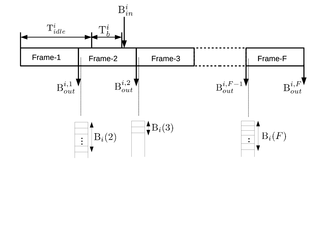
For example, number of bits at ’s buffer at the beginning of third frame duration as shown in Fig. 6, can be calculated as:
| (53) |
where, , is number of bits at ’s buffer at the beginning of second frame duration and bits . From Fig. 6, it can be observed that during second frame duration number of bits arrive at ’s buffer which we add in Equation (53). We assume identical values for .
For a particular frame duration, we correspond our simulation steps to different phases which we have shown in Fig. 2 as follows:
- •
After receiving all information from SUs, i.e., after Phase-1, as shown in Fig. 2, the FC finds optimal decision thresholds, optimal set for SUs from , and allotted time durations for selected SUs, following Algorithm 1, 2, 3, and 4, which are discussed in Section IV and V. Here, we assume that the FC is computationally powerful, such that, we can neglect the time for this evaluation process.
- •
The FC instructs selected SUs to perform spectrum sensing in Phase-2.
- •
In Phase-3, selected SUs perform spectrum sensing considering the sensing channel gain, i.e., , which we generate in a frame.
- •
After spectrum sensing, SUs send their hard decisions to the FC in Phase-4.
- •
The FC decides the PU to be idle when the summation of SUs’ decisions is less than the FC’s threshold as evaluated in Phase-1. The FC informs selected SUs about their allotted time durations in Phase-5.
- •
In Phase-6, selected SUs either access (with channel gains ) the licensed spectrum or remain idle based on the outcome in Phase-5. Please note that we consider actual rate (i.e., bits/sec.) for SUs, e.g., if the PU follows hypothesis and sensing outcome is , then rate for is considered as .
In Fig. 7, we plot average delays for SUs to clear their data from buffers for bits and bits, , while varying and .


Fig. 7(a) is for and dB, where we show that SUs take almost same time on average to clear their data from buffers for a given value of . SUs’ delays reduce for increasing the value for , which is intuitive. As the PU uses the licensed band less frequently, secondary network gets more chance to access the licensed spectrum without any interference from the PU. Therefore, SUs can clear their buffer data in less time.
Fig. 7(b) is for and dB, where we plot SUs’ average delays varying . As increases SUs take more time duration to clear their data from buffers due to less transmission opportunity to maintain stringent interference constraint. From both Fig. 7(a) and 7(b), it can be observed that SUs take almost same time to clear their buffer data for a given value of and , which indicates that our resource allocation algorithm is fair enough.
VI-C1 Fairness check
We further check the fairness of our algorithm following famous Jain’s formula as given following [34]:
| (54) |
In our case, corresponds to the delay for . We put average delay values received from Fig. 7(a) and 7(b) in Equation (54). Value of ranges from (worst case) to 1 (best case). We observe that for all values of and , we get .
VII Conclusion
In this paper, we have considered a joint spectrum sensing and resource allocation problem for an opportunistic cooperative CR network. The FC plays dual role, i.e., as global decision maker and resource allocator. In order to get resources, SUs pay to the FC. SUs are allocated different time slots by the FC to make the SUs’ transmission orthogonal over time. As the available time duration may not be sufficient for allocating time durations to all SUs, the FC may have to perform a selection procedure among SUs. Beside designing spectrum sensing thresholds, we also devise SU selection algorithm, which we prove optimal under certain condition.
Appendix A is not convex/quasi-convex over and
We first prove the first statementTo prove this, we consider . If we can show that is not quasi-convex over and , then we can conclude that is not convex/quasi-convex over and . To show this, we take help of bordered hessian matrix, which can be written for and as follows:
We describe elements of matrix in Equation (56a)-(56e), where,
For quasi-concavity, the following rules need to be maintained:
| (55a) | |||
| (55b) | |||
where,
| (56a) | ||||
| (56b) | ||||
| (56c) | ||||
| (56d) | ||||
| (56e) | ||||

It is observed that the condition as given in Equation (55a) always satisfies, however, the condition as given in Equation (55b), does not satisfy always. We consider an example considering dB, , , , and . We plot for varying in Fig. 8, where it can be observed that is not always positive. Therefore, we can conclude that is not quasi-convex/convex over and . As the objective function is not concave in lower dimension, we can conclude that the objective function is not concave in higher dimension also, i.e., for , , and .
The objective function and constraints of are linear functions of . Therefore, we can conclude that for given values for , and , the optimization problem belongs to convex optimization family.
References
- [1] V. N. I. Cisco, “Global mobile data traffic forecast update, 2015–2020 white paper,” Document ID, vol. 958959758, 2016.
- [2] Nokia, “Nokia lte for unlicensed spectrum.”
- [3] D. Malladi, “Best use of unlicensed spectrum,” 2016.
- [4] R. Zhang, M. Wang, L. X. Cai, Z. Zheng, X. Shen, and L.-L. Xie, “Lte-unlicensed: the future of spectrum aggregation for cellular networks,” IEEE Wireless Communications, vol. 22, no. 3, pp. 150–159, 2015.
- [5] M. AbdelRaheem, “Bargaining-based cooperative co-existence framework for lte-u systems,” in 2018 14th International Wireless Communications & Mobile Computing Conference (IWCMC). IEEE, 2018, pp. 1047–1052.
- [6] M. Mehrnoush, S. Roy, V. Sathya, and M. Ghosh, “On the fairness of wi-fi and lte-laa coexistence,” IEEE Transactions on Cognitive Communications and Networking, 2018.
- [7] M. D. Mueck, S. Srikanteswara, and B. Badic, “Spectrum sharing: Licensed shared access (lsa) and spectrum access system (sas),” Intel White Paper, 2015.
- [8] S. Kinney. Almost all spectrum is 5g spectrum. [Online]. Available: https://www.rcrwireless.com/20171006/5g/qualcomm-on-5g-spectrum-mix-tag17
- [9] J. Horwitz. Ericsson debuts spectrum sharing so 5g networks can run on 4g towers. [Online]. Available: https://venturebeat.com/2018/09/05/ericsson-debuts-spectrum-sharing-so-5g-networks-can-run-on-4g-towers/
- [10] S. Haykin et al., “Cognitive radio: brain-empowered wireless communications,” IEEE journal on selected areas in communications, vol. 23, no. 2, pp. 201–220, 2005.
- [11] H.-K. Lee, D. M. Kim, Y. Hwang, S. M. Yu, and S.-L. Kim, “Feasibility of cognitive machine-to-machine communication using cellular bands,” IEEE Wireless Communications, vol. 20, no. 2, pp. 97–103, 2013.
- [12] A. A. Khan, M. H. Rehmani, and A. Rachedi, “Cognitive-radio-based internet of things: Applications, architectures, spectrum related functionalities, and future research directions,” IEEE wireless communications, vol. 24, no. 3, pp. 17–25, 2017.
- [13] C. Liang and F. R. Yu, “Wireless network virtualization: A survey, some research issues and challenges,” IEEE Communications Surveys & Tutorials, vol. 17, no. 1, pp. 358–380, 2015.
- [14] H. Kim and K. G. Shin, “Admission and eviction control of cognitive radio users at wi-fi 2.0 hotspots,” IEEE Transactions on Mobile Computing, vol. 11, no. 11, pp. 1666–1677, 2012.
- [15] M. Sherman, A. N. Mody, R. Martinez, C. Rodriguez, and R. Reddy, “Ieee standards supporting cognitive radio and networks, dynamic spectrum access, and coexistence,” IEEE Communications Magazine, vol. 46, no. 7, 2008.
- [16] S. Bhattarai, J.-M. J. Park, B. Gao, K. Bian, and W. Lehr, “An overview of dynamic spectrum sharing: Ongoing initiatives, challenges, and a roadmap for future research,” IEEE Transactions on Cognitive Communications and Networking, vol. 2, no. 2, pp. 110–128, 2016.
- [17] T. Yucek and H. Arslan, “A survey of spectrum sensing algorithms for cognitive radio applications,” IEEE communications surveys & tutorials, vol. 11, no. 1, pp. 116–130, 2009.
- [18] G. Ganesan and Y. Li, “Cooperative spectrum sensing in cognitive radio networks,” in New Frontiers in Dynamic Spectrum Access Networks, 2005. DySPAN 2005. 2005 First IEEE International Symposium on. IEEE, 2005, pp. 137–143.
- [19] S. M. Mishra, A. Sahai, and R. W. Brodersen, “Cooperative sensing among cognitive radios,” in Communications, 2006. ICC’06. IEEE International conference on, vol. 4. IEEE, 2006, pp. 1658–1663.
- [20] J. Unnikrishnan and V. V. Veeravalli, “Cooperative sensing for primary detection in cognitive radio,” IEEE Journal of selected topics in signal processing, vol. 2, no. 1, pp. 18–27, 2008.
- [21] R. Fan and H. Jiang, “Optimal multi-channel cooperative sensing in cognitive radio networks,” IEEE Transactions on Wireless Communications, vol. 9, no. 3, 2010.
- [22] R. Fan, H. Jiang, Q. Guo, and Z. Zhang, “Joint optimal cooperative sensing and resource allocation in multichannel cognitive radio networks,” IEEE Transactions on Vehicular Technology, vol. 60, no. 2, pp. 722–729, 2011.
- [23] S. M. Almalfouh and G. L. Stuber, “Uplink resource allocation in cognitive radio networks with imperfect spectrum sensing,” in Vehicular Technology Conference Fall (VTC 2010-Fall), 2010 IEEE 72nd. IEEE, 2010, pp. 1–6.
- [24] R. Xie, F. R. Yu, and H. Ji, “Dynamic resource allocation for heterogeneous services in cognitive radio networks with imperfect channel sensing,” IEEE transactions on vehicular technology, vol. 61, no. 2, pp. 770–780, 2012.
- [25] H.-J. Lim, D.-Y. Seol, and G.-H. Im, “Joint sensing adaptation and resource allocation for cognitive radio with imperfect sensing,” IEEE Transactions on Communications, vol. 60, no. 4, pp. 1091–1100, 2012.
- [26] S. Wang, Z.-H. Zhou, M. Ge, and C. Wang, “Resource allocation for heterogeneous cognitive radio networks with imperfect spectrum sensing,” IEEE Journal on Selected Areas in Communications, vol. 31, no. 3, pp. 464–475, 2013.
- [27] A. Shahini and N. Ansari, “Joint spectrum allocation and energy harvesting optimization in green powered heterogeneous cognitive radio networks,” Computer Communications, 2018.
- [28] W. Ejaz and M. Ibnkahla, “Multi-band spectrum sensing and resource allocation for iot in cognitive 5g networks,” IEEE Internet of Things Journal, vol. 5, no. 1, pp. 150–163, 2018.
- [29] K. Kulkarni and A. Banerjee, “Multi-channel sensing and resource allocation in energy constrained cognitive radio networks,” Physical Communication, vol. 23, pp. 12–19, 2017.
- [30] N. Biswas, G. Das, and P. Ray, “Optimal hybrid spectrum sensing under control channel usage constraint,” IEEE Transactions on Signal Processing, 2018.
- [31] K. Fitchard. Hotspot 2.0 inches its way into public wi-fi networks. [Online]. Available: https://gigaom.com/2014/03/07/hotspot-2-0-inches-its-way-into-public-wi-fi-networks/
- [32] Y.-C. Liang, Y. Zeng, E. C. Peh, and A. T. Hoang, “Sensing-throughput tradeoff for cognitive radio networks,” IEEE Transactions on Wireless Communications, vol. 7, no. 4, pp. 1326–1337, 2008.
- [33] P. K. Varshney, Distributed detection and data fusion. Springer-Verlag New York, Inc., 1996.
- [34] R. K. Jain, D.-M. W. Chiu, and W. R. Hawe, “A quantitative measure of fairness and discrimination,” Eastern Research Laboratory, Digital Equipment Corporation, Hudson, MA, 1984.