Model interpretation through lower-dimensional posterior summarization
Abstract
Nonparametric regression models have recently surged in their power and popularity, accompanying the trend of increasing dataset size and complexity. While these models have proven their predictive ability in empirical settings, they are often difficult to interpret and do not address the underlying inferential goals of the analyst or decision maker. In this paper, we propose a modular two-stage approach for creating parsimonious, interpretable summaries of complex models which allow freedom in the choice of modeling technique and the inferential target. In the first stage a flexible model is fit which is believed to be as accurate as possible. In the second stage, lower-dimensional summaries are constructed by projecting draws from the distribution onto simpler structures. These summaries naturally come with valid Bayesian uncertainty estimates. Further, since we use the data only once to move from prior to posterior, these uncertainty estimates remain valid across multiple summaries and after iteratively refining a summary. We apply our method and demonstrate its strengths across a range of simulated and real datasets. Code to reproduce the examples shown is avaiable at github.com/spencerwoody/ghost.
Keywords: decision theory, graphical summary, interpretable machine learning, nonparametric regression, partial effects
1 Introduction
In regression modeling, there has traditionally existed a natural tension between model flexibility and interpretability. Consider the generic regression model given by
| (1) |
There are many models available to estimate the function , which describes the relationship between the covariates and the expected outcome of the noisy observations . On one hand, simple models such as the linear model or a shallow regression tree are readily interpretable, but are likely biased because they cannot capture complex relationships between the input and the response. On the other hand, more complex nonparametric regression models can yield highly accurate predictions but are difficult to interpret.
In particular, we often would like to answer questions such as: which covariates have the strongest effect on prediction? Does covariate importance differ across the covariate space? Are there interactions among the covariates, and if so, which are most important? Answering such questions is difficult, and providing appropriate measures of uncertainty is even more so.
In this paper, we propose an approach to give interpretable model summaries designed to answer such questions. We assume a Bayesian vantage point throughout, so that a flexible prior is specified for the regression function and the posterior is calculated by conditioning on observed data. The key idea of our approach is to follow a two-stage process. First, specify a flexible model for and use all the available data to best estimate this relationship. Second, perform a post hoc investigation of the fitted model using lower-dimensional surrogates which are suited to answer relevant inferential questions and sufficiently representative of the model’s predictions. These summaries are functions of , so obtaining their posterior distribution is straightforward. This investigation in the second stage is simply an exploration of the posterior for . The result is a set of interpretable explanations of model behavior, along with posterior distributions for these explanations, which are valid in the sense that we condition on the data only once (in calculating the posterior for ).
The methods we develop are highly modular, allowing for a variety summaries to interpret many possible regression models. Here we demonstrate three particular uses of posterior summarization which we believe to be widely advantageous and represent valuable contributions, including (i) to efficiently and intuitively describe partial effects, (ii) to communicate the most significant interactions detected by the first-stage regression model, and (iii) to describe how the predictive importance of covariates changes across local areas of the covariate space. Because we take a Bayesian approach, these summaries all come with posterior uncertainty estimates.
The remainder of the paper is structured as follows. In the rest of this section we develop our decision theoretic approach for producing model summaries, and describe several metrics for gauging the how well model summaries explain model predictions. In Section 2 we consider the case of estimating and quantifying posterior uncertainty in lower-dimensional summaries for linear models. This leads us into Section 3 where we generalize this approach to summarize nonparametric regression models. In Section 4 we present simulation results which show how our method of nonparametric regression summaries can accurately communicate the average partial effects of covariates and convey significant interactions present in a fitted regression model. We apply our method to a real data example in Section 5 by presenting an extensive case study interpreting a predictive model for housing prices in California. We conclude with a discussion in Section 6.
1.1 Separating modeling and interpretation
Our goal is to produce interpretable summaries of regression models. Equivalently, we wish to understand important predictive trends in the regression function from Eq. (1). To do so, we consider a lower-dimensional class of functions that can be used for parsimoniously characterizing . We can summarize by finding a that closely matches its predictions. Formally, we let be the function minimizing an objective defined by
| (2) |
where measures discrepancy in prediction between the original high-dimensional model and the parsimonious summary over some specified covariate locations of interest , and is an optional penalty function measuring complexity in governed by one or several tuning parameters . The penalty may be used, for instance, to enforce sparsity or smoothness in the summary. Now the summary is the function minimizing this objective,
| (3) |
Of course, we do not know the true regression function , but rather have a posterior distribution for it. Because here is a functional of the regression function , it has a posterior implied by that of . That is, the posterior of is precisely the posterior distribution of the best approximation of in the class as measured by the penalized predictive discrepancy in (2).
For example, if is the set of linear functions and there is no penalty , then we obtain the posterior distribution of the best linear approximation to , thereby describing the average partial effects of covariates on the conditional expectation of the outcome. We obtain this directly, without fitting a misspecified linear model for the outcome from the outset. We can also simultaneously consider linear summaries in variables, additive summaries, and so on, all with valid Bayesian inference.
The summary objective (2) is flexible by design, allowing to be any set of chosen covariate locations, possibly with different weights assigned within the discrepancy function . If it is chosen to be the entire dataset, then the result is a global summary of model predictions. If is a subset of the data confined to a restricted region, the result is a local summary of model predictions within this region. This is particularly helpful, as nonparametric regression models naturally adapt to local heterogeneity in covariate importance; for instance, in Section 5.2 we illustrate how the determinants of housing prices vary geographically. If is chosen to be a set of locations where the outcome has not been observed, then the summary explains how the model makes predictions at these new locations.
This distribution for given by (3) accounts for uncertainty in the summary function, but leaves open the question of a point estimate. Using standard Bayesian decision theory (Berger 2013, e.g., ), if we cast the objective function (2) as a loss function then the optimal point estimate for the summary is that which minimizes posterior expected loss, i.e.
| (4) |
with this expectation taken over . When is chosen to be squared-error, then the point summary is equivalent to minimizing the loss function in (2) with the posterior mean taking place of , and so the point estimate becomes
This form conveniently lends itself to the use of many standard estimation procedures, where the summary estimate is obtained from the fitted values of . The tuning parameter(s) may be selected using usual approaches adapted for this case, e.g. using cross-validation on the values of .
Here we pause to emphasize the subtle distinction between the point estimate in (4) and the posterior for the summary given by (3). The former is the point estimate (more precisely, the Bayes estimate) of the summary, while the latter is the entire posterior for the lower-dimensional characterization of . This is akin to the difference between the Bayes estimator for a scalar parameter, and the posterior for that parameter. The posterior mean of is not necessarily equivalent to , i.e. in general
Our work is related to that of Crawford et al. 2018; Crawford et al. 2019 who calculate linear projections of nonlinear regression models to produce an “effect size analog” for each covariate. Here, however, we allow for a more general set of possible summaries, and introduce heuristics to iterative update a summary to produce a more faithful representation of the regression model. Additionally, we extend and generalize previous approaches which derive decision-theoretic point estimate model summaries; for example, Hahn and Carvalho 2015 introduce posterior summarization for communicating dominant trends in linear models. This framework has been shown to be effective in a variety of modeling contexts (Puelz et al. 2017; Chakraborty et al. 2019; Puelz et al. 2015; Puelz et al. 2019; Bashir et al. 2018; Kowal and Bourgeois 2020; MacEachern and Miyawaki 2019; Lee and MacEachern 2014). Related ideas in this direction can be traced back to MacEachern 2001 who developed linear summaries for nonparametric regression models.
1.2 Summary diagnostics
A natural concern after summarization is the adequacy of the summary function approximation to the regression function. The summary will generally have less predictive power than because it sacrifices flexible predictive features in such as nonlinearities or interactions. There are several ways one may gauge this.
We propose two diagnostic metrics to quantify the sufficiency of summarization. The first measures predictive variance in the original model explained by summarization,
where . This is the “summary .” The second metric, which can be used for the case of normal errors, is
where is the observation corresponding to . This metric has the loose interpretation that using the summary model increases the width of predictive intervals by . If the observations are not available, then we can use estimates from the posterior predictive . Similar quantities may be calculated for non-normal errors. Both of these metrics also come with posterior distributions, calculated by using posterior draws of , , and .
Furthermore, one can visually inspect the “summary residuals” , either with a scatter plot or fitting a single regression tree, which could reveal important interactive effects in driving variation in the summary residuals that should be considered.
After analyzing the summary model in this way, either quantitatively with these two metrics or qualitatively through the summary residuals, we may be determine that the class of summaries was too simplistic to satisfactorily explain the original model. Then it is appropriate to specify a more nuanced class of summary, such as one which allows for interactions, or one that allows for nonlinear rather than linear effects. This suggests an iterative approach of progressively assessing and updating the class of summaries until one or more summaries is deemed to be sufficiently representative of the original model’s predictions. Critically, our summarization and posterior projection approach still yields valid Bayesian inference after this “summary search.” We detail this iterative approach in Section 3.
2 Lower-dimensional summaries in the linear model
We first consider the relatively simple case of summarizing a high-dimensional linear model with a subset of the variables. We extend the work of Hahn and Carvalho 2015 by introducing measures of uncertainty in the summary via posterior projection.
The full model is a standard multiple linear regression, , with independent priors We wish to find a sparse set of relevant features. Denote this set by the inclusion vector . Using the notation introduced in the previous section, this is equivalent to replacing the original fitted function with the summary for a sparse vector , where if . If we use the squared-error function to measure predictive discrepancy and some sparsity-enforcing penalty (Tibshirani 1996, such as the penalty of) then the optimal sparse summary point estimate is
| (5) |
where is the posterior mean of . Note that this matches Eq. (20) of Hahn and Carvalho 2015. The penalty term is included solely for sparsity in the solution. For any such penalty, (5) returns an entire solution path for possible sparse summaries of the original high-dimensional model, with the level of sparsity varying with the tuning parameter .
After solving (5) for some fixed value of , we have sparse set of coefficients which is a Bayes-optimal point estimate summary for the full model. Using our posterior projection technique, we can also quantify uncertainty in this summary. A naive approach would be to refit the model only with the selected covariates. However, this would involve using the outcome data a second time—an example of “posterior hacking,” or opportunistically retraining a new model after already conditioning on the data once in the original model.
Instead, it is more appropriate to propagate posterior uncertainty from the original fitted model through to the linear summary. The sensible way to do this is to take the full posterior distribution for the fitted function of the full model using all the variables, and project it onto the space of the fitted summary function using the restricted set of variables. We use the data exactly once (in obtaining the posterior for the original full model) and obtain the posterior of the best linear approximation in variables.
To be more specific, for one value of , denote the corresponding sparse model summary with the inclusion vector , whose th element is 0 if and 1 otherwise. Given a sparse linear summary specified by (for notational simplicity, dropping the subscript), we want to give a coherent posterior distribution to the included coefficients. This is the posterior for the low-dimensional linear representation of the original model.
Let denote the -subset of the columns of the original covariate matrix , and let be the vector of coefficients for this restricted covariate matrix. We wish to map the posterior for , the original fitted values, onto , the fitted values using the restricted set of coefficients. This is equivalent to projecting the original fitted values onto the column space of . We can approximate the posterior distribution for the restricted covariates via Monte Carlo, i.e., for the th draw from the original posterior, , perform the projection
| (6) |
assuming the inverse exists. For this reason, we call the the “projected posterior.”
In this way we can obtain projected posteriors for all sparse summary models from the solution path given by (5), and report the summary which is sufficiently representative of the original full model’s predictions, as measured by the summary diagnostic measures given in Section 1.2. We emphasize that in (5) is the Bayes-optimal point estimate for the summary, and the projected posterior represents posterior uncertainty around this estimate.
2.1 Sparse linear summaries for the US crime data
Here we illustrate our approach of quantifying uncertainty in sparse linear summaries on the US crime dataset, which has observations with predictors. We fit a linear model using the horseshoe prior (Carvalho et al. 2010) after log-transforming the continuous variables, and centering and scaling all variables. Then we obtain point estimates for linear summaries of the full model by solving the minimization problem in (5). Because the posterior mean is already a shinkage estimator due to the influence of the prior, we use the adaptive lasso penalty (Zou 2006) for the penalty term, with to alleviate the problem of “double shrinkage” that would result from using the usual (unweighted) penalty. These summaries were calculated using the lasso implementation from the lars package (Hastie and Efron 2013) in the R programming language (R Core Team 2019). For each point estimate summary, we calculate its projected posterior following (6).
Figure 1 shows posterior distributions for the summary diagnostics defined in Section 1.2 for the entire solution path of sparse linear summaries. Following Hahn and Carvalho 2015, we recommend reporting the summary model with 6 predictors included, as this summary explains approximately 95% of predictive variation in the full model, and predictive intervals are inflated by only about 5% on average. However, the summary diagnostics allow an analyst to pick any reasonable tradeoff between parsimony and predictive ability, and we can get valid inference for any summaries of interest.
We use this example to consider the effect of sparsification on the shape of projected posteriors. Figure 2 investigates the projected posteriors for two highly collinear variables, Po1 and Po2, as the linear summary becomes more parsimonious. The presence of collinearity results in both covariates having high posterior variance in the full model, and due to the nature of the horseshoe prior which aggressively shrinks variables near zero while retaining heavy tails, both marginal posteriors are bimodal with modes near and away from zero. However, moving from the summary with 10 variables to the summary with 9 variables (when Po2 is “selected out” of the summary), the projected posterior mode for Po1 near zero disappears, and all the mass in the posterior is shifted to the right. This shows the gain in power from using our summarization approach. Projected posteriors for all variables for all summaries shown in the supplement.
Finally, in Figure 3 we compare the projected posterior for the final selected sparse summary model to the posterior we would obtain by refitting the linear model only including these variables, instead of projecting the posterior draws. For this case we now use a flat prior on (the restricted vector) as we suspect that there is less need for shrinkage since we have reduced the dimensionality. In this second case, we are “double dipping” with the data, using it once to fit the full model, and then using it a second time after the sparse linear summary is chosen. This inference is not strictly valid, since the data are used here to set the prior by selecting the restricted set of variables. More importantly, this posterior entirely ignores model uncertainty. By comparison, the projected posterior uses the response variable only once, in calculating the posterior for the full model. We also show the marginal posteriors from the original fitted (saturated) linear model.
The projected posteriors are wider than the refitted posteriors, due to the propagation of model uncertainty. The projected posteriors retain the shrinkage properties of the original posterior: the posterior means for each variable are shrunk toward zero compared to the refitted posterior. In most cases the projected posteriors closely match the marginal posteriors of the full model, the biggest exception being Po1 for the reasons just discussed.
3 Summaries for nonparametric regression
We now move to our main topic: summarization of nonparametric regression models. This problem is more nuanced than for the linear model, where increasing summary complexity was well defined by the dimension of the sparse linear summary. Here, however, it is less clear how to define a collection of increasingly complex summaries from which to choose. This suggests an iterative approach, whereby an initial summary is proposed, calculated, evaluated and updated as necessary.
Before an presenting investigative simulation examples in Section 4 and an extensive case study in Section 5, we describe heuristics for model summary search. This is given in detail below, with Algorithm1 containing a brief outline of our procedure. The exposition is intentionally general, meant to allow for any class of regression models with any error distribution, and any class of lower-dimensional summaries corresponding to inferential goals of interest. We also describe how this approach can be used to elucidate how the model predicts globally or locally. Exact details of how to processed will be heavily context dependent, influenced by the specific dataset, original specified model, and the inferential target.
3.1 Iterative summary search
(1) Specify and fit the full model.
Assume the regression setting described by
and complete the model specification by assigning priors for the regression function as well as any nuisance parameters. Our approach is agnostic to the choice of , though we do assume that it fits well by adequately modeling the response as a function of the covariates . Typically this should be a nonparameteric prior, such as a Bayesian tree ensemble (Chipman et al. 2010) or some variant of a Gaussian process (Gramacy and Lee 2008; Gramacy and Apley 2015, e.g.).
We obtain Monte Carlo draws targeting the posterior of , denoted by . Denote the posterior mean for the fitted value of the function at by .
(2) Summarize.
Choose a class of summaries which matches the inferential goal at hand. For example, if the objective is to comment on the partial linear effect of each covariate, then is chosen to be linear. If instead the goal is to simply comment on the partial effect of each covariate, without the constraint of linearity, then one can choose to be the broader class of additive functions.
We also need to specify the predictive locations at which to summarize the model output, a metric for measuring predictive discrepancy between the summary and the full model, and an appropriate summary complexity penalty function . These components collectively define the summarization loss function
The optimal point summary is
found by minimizing the summarization loss in expectation over the posterior for . Tuning parameters can be determined, for example, through cross-validation or use of information criteria on the posterior mean fitted values . Once has been calculated, the posterior distribution for the summary can be found by the posterior of the functional . Often this will involve projecting posterior draws of the fitted values onto the predictive space of .
(3) Evaluate.
Next, assess the impact of moving from the full model to the low-dimensional summary. The summarization metrics and defined in Section 1.2 offer two readily interpretable ways to quantify this loss in predictive power. One may also inspect the summarization residuals, directly, for example by training a regression tree to these residuals to detect and characterize heterogeneity.
(4) If the summary is sufficient, perform inference.
Based on the results from Step (3), determine whether the summary model is sufficient. For example, if is reasonably high and the summarization residual regression tree does not detect large amounts of residual heterogeneity, then the calculated summary in Step (2) may be judged to be of good quality and representative of the model’s predictions, and so this summary may be used for the inference stage. Ultimately it is left to the end user to make a decision regarding sufficiency of the calculated model summary.
(5) Otherwise, refine and return to (2).
If the summary is deemed to be of poor quality, there are two ways to improve model summary accuracy: the class of summary models can be enriched to allow for greater flexibility, or the predictive locations can be altered to be more localized. The choice of one or both of these options can be informed by the evidence provided from the evaluation procedure in Step (3). For instance, if the regression tree detects high levels of heterogeneity in the summarization residuals, one may allow for low-order interactions determined by splitting rules near the root of the tree.
With these new classes of summaries, and/or designated predictive locations, return to Step (2) to calculate the summary and iterate through all these steps until a summary is deemed sufficient or it is judged that no summarization class can be specified that is representative enough of the model’s predictions while still being interpretable. We need not constrain ourselves to a single model summary, however; we may compute multiple summaries to interpret of model behavior, and these will all have valid Bayesian posteriors.
-
[(1)]
- 1.
Specify and fit the model
- •
Give a prior for .
- •
Obtain posterior samples for the model,
- •
Choose an initial class of summaries , complexity penalty (if desired) and predictive locations , collectively defining the summary loss .
- •
- 2.
Summarize
- •
Calculate the optimal point estimate for the summary
- •
Calculate the projected posterior for the summary using posterior draws of
- •
- 3.
Evaluate
- •
Compute summarization metrics and
- •
Inspect the summarization residuals with a decision tree
- •
- 4.
Iterate if necessary
- •
If the summary is deemed satisfactory by metrics in (3), use this summary for interpretation.
- •
Otherwise, change the class of summaries and/or predictive locations , and iterate through (2) and (3)
- •
4 Simulation results
4.1 Estimating and visualizing partial effects
Here we present a toy example to illustrate how our approach can be used to estimate partial effects as a summarization of a nonparametric regression model. We simulate data from the model
centered on the bivariate nonadditive function defined by
with , and observations along a regular 2D grid of values over the range . No other covariates are observed or used to generate the data. Using these data we estimate by using a Gaussian process (GP) prior with a squared exponential covariance kernel, and assign Jeffreys’ prior for .
We consider two summaries to explain model predictions in the GP posterior for by estimating the partial effect of each covariate. The first is a linear summary, so the class of summaries is the set of functions of the form . The second is an additive summary, so the class of summaries is the set of functions of the form , with and being univariate functions whose forms we discuss in the proceeding paragraph. Here and throughout the paper, we use the squared error predictive discrepancy function, so the summary loss functions are
with , is the complexity penalty in the additive summary, and enforces smoothness in the univariate functions and . The tuning parameters and control the level of smoothness. We do not add a penalty for the linear summary. The point estimates for these summaries are found by minimizing posterior expected loss,
| (7) | ||||
| (8) |
The point estimate for the linear summary can be found via an ordinary least squares fit to the vector of fitted values , i.e. . We find the projected posterior for the linear summary using posterior draws of , so that one draw from the projected posterior is .
The functions and for the additive summary are represented by thin plate regression splines (Wood 2003, TPRS;) each with a basis dimension of 10, with the identifying constraint for all . Each function is represented by the linear basis expansion,
where the are the basis functions, and each function has basis terms. The entire vector of output from the additive model is given by , where the th row of the matrix represents the linear basis expansion of , , and is the concatenation of the basis weights. The point estimate for the additive summary (8) is found by estimating iteratively reweighted least squares, with the tuning parameters and selected by minimizing the generalized cross validation score on the values of . In our implementation, we use the default settings of the gam function in the mgcv package in R. For details on the form of the basis functions and how the model is fit, see Wood 2003; Wood 2017. The particular choice of basis expansion is not of main concern here, and any suitable basis will do.
In the end, the vector fitted values for the point estimate additive summary (8) can be represented by a linear smoothing of the posterior mean fitted values from , i.e. , with the influence matrix calculated by where being the frequentist covariance matrix of the estimates . In fact, the fitted values evaluated for each of the additive functions are the result of a linear smoother, i.e. , where is the subset of rows of the projection matrix corresponding to the basis expansion for the th term. This readily provides a way to approximate the projected posterior for each smooth function in the additive summary using posterior draws of original fitted values . A single posterior draw from the projected posterior is calculated by .
Figure 4 shows the resulting summaries. Panel (a) shows the true regression function and the observations, and compares them to the estimated regression function from the GP model, and to the bivariate surface resulting from the summary functions. These summaries have differing degrees of fidelity in capturing predictive trends in the original model; for the linear summary, and while for the additive summary, and . Panel (b) shows the estimated partial effects of each summary, along with 95% credible bands from the projected posterior.

These summaries estimate of the partial effect of each covariate. Equivalently, they approximate the partial derivative of the true regression function, with the (incorrect) simplifying assumption that the partial derivative is constant in the other covariate (or constant everywhere in the case of the linear summary). Panel (c) shows the partial derivatives with respect to and of the true, estimated, and summary functions as a bivariate function of . From this we can see that the summaries present distinct ways of averaging the partial derivative from the estimated regression function in a way that is readily presentable and interpretable as partial effects in Panel (b). We also quantify how representative these summaries are of the original model with the diagnostic measures.
4.2 Interaction detection in the presence of collinearity
The previous example showed how our method of posterior summarization can communicate average partial effects. Now we present a simulated example with a more complex data structure to show how we can detect significant interactions within a regression model, even in the presence of collinear noise covariates, by using the iterative summary search heuristics outlines in Section 3. We consider data arising from the following:
| (9) | ||||
The true data generating process in Eq. (9) involves 3 variables , with one interaction between and . For this simulated example, we also observe 3 noise covariates which are not involved in the data generating mechanism, but are still correlated with the other features. To induce correlation between the features, we generate the vector of covariates from the multivariate Gaussian distribution:
with . This reflects weak to moderate correlation between the signal and noise covariates. The two interactive features are are uncorrelated, but both are correlated with the remaining signal feature . We generate covariate vectors of from this Gaussian distribution to create the design matrix , and generate observations using the process in Eq. (9). As in the previous example, we estimate the regression function using a Gaussian process with a squared exponential kernel and assign Jeffreys’ prior to . We obtain draws from the posterior for .
To describe the predictive trends detected in the posterior for the model , we first construct an additive summary of the form . This summary and its projected posterior are calculated in the same way as in the previous example, and these are presented in Figure 5. To see how well this summary describes the fitted model, we first we consider the predictive variance explained by the summary, which is in this case, suggesting that there is considerable amount of variation in the posterior for that is not being captured by this summary. Second, because this summary assumes additivity in the covariates, we can detect significant sources of unexplained variation due to interactions by constructing a single decision tree regressing the summarization residuals on all the observed covariates. This tree is shown in the supplement, and the pairs of covariates in neighboring nodes of this tree suggest prospective significant interactions detected by the model which should be accounted for.
To create a more faithful summary of the fitted function, we consider summaries which allow for a two-way interaction between two of the covariates, leaving the summary function additive in all the other covariates. That is, the summary class is , the set functions of the form . This summary function is partially additive, allowing for a single two-way interaction via the bivariate function , represented as a two-dimensional thin plate regression spline with basis dimension 30. The summary loss function in this case is
with the penalties defined before, and now enforcing smoothness in the bivariate function. For details of higher-order TPRS penalty functions we again refer the reader to Wood 2003; Wood 2017. The point estimate summary and projected posterior for are found analogously to those of the purely additive summary.
The relevant question is the choice of which interaction to add, which should be the most significant interaction present in the fitted model. We could narrow our attention to considering in interactions between the pairs of covariates detected by the suggested by the summary residual regression tree, but for the sake of completion, we fit the summary for each possible pair of covariates. Whichever interaction pair leads to the greatest increase in should indicate which interaction is most significant in the model.
The values for these partially additive summaries are show in the bottom row of Figure 6. The interaction between and gives by far the biggest gain in predictive variance explained as measured by compared to every other possible two-way interaction, with this metric rising to about . This confirms that the interaction for is the most important one detected by the GP model for . The resulting partially additive model summary with an interaction for this simulation is shown in Figure 7.
This pattern is routinely detected across multiple replications of this simulation example; when replicating this simulation up to 1000 times, the interaction gives the largest boost in at a rate of 98.9% (SE = 0.3%). The values for twenty of these additional replications are given in Figure 6, with the comprehensive set of results presented in the supplement. This suggests that our method is able to recapitulate the interaction which is present in the true data generating process when summarizing a Gaussian process regression, even in the presence of correlated noise variables. Note that this results hinges on the specified regression model being able to accurately capture the interaction between the covariates.


5 Application to California housing data
Here we demonstrate our approach using data from the 2011 American Community Survey on housing prices in California at the census tract level. We regress census tract log-median house value on log-median household income, log-population, median number of rooms per unit, longitude, and latitude, using a Gaussian process regression model. The full model is given by
where is the log-median house value and is the covariates for census tract . We use a combination of squared exponential kernel and the linear covariance kernel,
for the predictors. Empirical Bayes estimates for , , , and were found using maximum marginal likelihood estimation. We obtained posterior draws for and using MCMC after fixing the GP hyperparameters to the estimated values , , and . Denote by the vector of fitted values at all covariate locations in the dataset for the th Monte Carlo posterior draw of , for . The GP model can account for nonlinear and interactive effects of covariates on housing prices, and because of this flexibility, we achieve a good quality of fit as measured by the usual coefficient of determination, .
However, the output of the fitted GP model alone has little utility for qualitatively understanding the influence of each covariate. To better understand the fit, we calculate several summaries for this regression model, each representing different characterizations of the relationship between the covariates and the output, as an illustration of the iterative approach outlined in Section 3. We leave out most of the technical details of calculating the summaries, as they closely mirror those of the simulation examples in Section 4.
We first consider global summaries of model behavior, showing how the class of summaries can be refined until it is deemed a satisfactory representation of the original model’s predictions, and also how this process can reveal important interactive effects in the housing price model. Then we compute local summaries of model behavior, investigating how determinants of housing prices differ geographically. We only consider linear summaries for explaining local behavior, but demonstrate how adjusting the level of locality detects heterogeneity in covariate importance between these local areas.
5.1 Global summary search
5.1.1 Global linear summary
We start by creating a linear summary for the fitted model, perhaps the simplest summary one could make of a nonparametric regression. The summary function has the form . The vector represents the average partial effect of each covariate. There is no penalty term used here (imposing linearity is already a significant restriction), but one could just as easily use a penalty term if a sparse linear summary is desired. The point estimate and projected posterior for the linear summary are calculated in a parallel manner to those from the simulation example in Section 4.1.
Figure 8 shows the results of the projection and, compared to the results of fitting an ordinary least squares (OLS) regression of on . On average, the projected credible intervals for the coefficients in the linear summary are about 30% narrower than the 95% confidence intervals from OLS. Also, point estimates are generally closer to zero for the linear summary than for OLS, likely due to a shrinkage effect from the GP prior. In a sense, this is precisely what we would expect to see. The linear summary is the best linear approximation to the fitted function from the GP, without assuming that the response surface is actually linear. Furthermore, the linear summary is a projection of the fitted values from , which have lower variance than the observations used for creating the OLS estimates.
The diagnostics for this linear summary are shown in Figure 9, along with those from several other fitted summaries (which will be described later). The linear summary explains about of the variation in the predictive model, and residual standard deviation is inflated by about . This reflects a rather poor summary representation of the model, and suggests that there is important variation in the regression model that is being unaccounted for. While this summary is indeed the best linear approximation to the fitted regression model, we are evidently missing out on important features of .
5.1.2 Global additive summary
The requirement of linearity is rather limiting for summarizing the fitted GP regression, so we remove this constraint and consider instead the larger class of additive functions. Instead of a describing the partial effects of covariates on housing pricess linearly, we now describe partial effects with smooth nonlinear functions. That is, the summary class comprises functions of the form
| (10) |
and, again as in the simulation example in Section 4, each function has a thin plate regression spline representation with basis dimension 10.
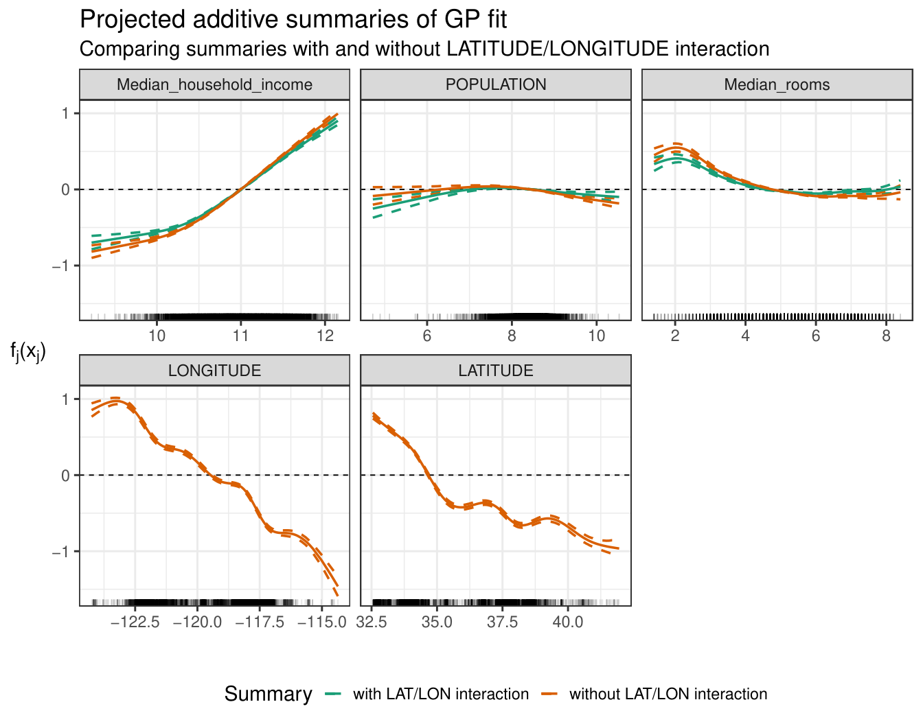
The point estimate and 95% credible bands for this additive summary are represented by the orange lines in Figure 10. Diagnostics for this summary are shown in the second column of Figure 9. Compared to the linear summary, the additive summary (10) represents a significant gain in predictive explainability as measured by both , rising from to , and , dropping from to .
Still, the assumption of additivity is quite a strong one for summarizing the fitted GP regression. There may be significant underlying interactions in the original model which we are missing here. To investigate this possibility, we fit a regression tree to the summary residuals truncated to a maximum depth of four for ease of presentation (shown in the supplement). The tree detects a high degree of heterogeneity in the summary residuals, so we next consider allowing for interactions in our summary.
Interaction search
Analysis of the summary residuals from the additive summary suggests that we should refine the summary to allow for some low-level interaction among the covariates. Specifically, it appears that longitude and latitude have the most important interactive effect, as these covariates appear highest in the summary residual regression tree. For the sake of completeness, we will also consider interactions involving median rooms and log-median household income, as these covariates also appear in the regression tree (even though very few data points fall into the nodes corresponding to these covariates; we do exclude the log-population covariate from consideration, as the node containing this variable contains a vanishingly small proportion of data points).
We will initially consider adding a single two-way interaction to the summary, using every possible pairing of these four covariates. Then we will move along a path of increasing summary complexity, adding a second two-interaction, and finally considering an additive summary with a three-way interaction.
Including a single two-way interaction, is now to the set of partially additive functions
| (11) |
where is a two-dimensional smooth function for the interaction, constructed using a two-dimensional thin plate regression spline with basis dimension 30.
Figure 9 contains the summary diagnostics for all the considered configurations of the partially additive summary (11) using the specified covariates. As suggested by the summary residual regression tree, the additive summary interacting longitude and latitude marks the best improvement by far in predictive explainability, marking a rise in from to and a fall in from to as compared to the original (non-additive) summary. That this is the most significant interactive effect is not surprising, as geography likely plays a large role in explaining housing prices in a way that is not separable by latitude and longitude. The fitted summary, accompanied by 95% credible bands, is shown in Figure 10 in comparison to the previously fitted non-interactive additive summary.
Again, we look for the possibility of an important unaccounted interactive effect by fitting a regression tree to the summary residuals from this newly calculated summary (shown in the supplement). Longitude and latitude seem to remain the most significant source of summary residual heterogeneity, possibly implying that the fitted two-dimensional smooth function in the interactive additive summary was oversmoothed. However, we turn our attention now to possible interactions between median household income and the spatial covariates, which are implied by this second summary residual regression tree.
We consider introducing a second two-way interaction in addition to the longitude-latitude interaction. That is, we consider two summaries, including (i) a summary allowing for interactions for longitude-latitude and longitude-income, and (ii) a summary allowing interactions for longitude-latitude and latitude-income. However, neither of these summaries mark a significant improvement over the summary with a single two-way interaction, demonstrated by the fact that the posteriors for the summary diagnostics of these two models overlap with that of the partially additive summary with only the longitude-lattitude interaction, seen in Figure 9.
The next step up in the progression of summary complexity is to accommodate a three-way interaction for longitude-latitude-income (i.e., a three-dimensional smooth). Looking at the summary diagnostics for this fitted summary, we do now notice a significant gain in predictive explainability over the partially additive summary with a single interaction for longitude-latitude. But choosing this summary model would require a large sacrifice in interpretability of the summary for a relatively low gain in predictive ability.
Therefore, we conclude the summary model with one interaction between latitude and longitude is most appropriate to report. It has an value of about and a value of about , which is considerable given the level of complexity which the original GP regression model is able to accommodate. Thus, we can conclude that the trend in housing prices as explained by the covariates is somewhat close to additive, with an important interaction between longitude and latitude, although some more complex features remain.
5.2 Local linear summaries
To draw out some of these features, we consider local behavior of the regression function . Previously we focused on global model summaries, capturing how the model behaves on average across the entire dataset. However, one of the advantages of nonparametric regression is that the model adapts to heterogeneity in the response surface. That is, covariate importance is likely to be nonconstant across the covariate space. This applies in our example; it is likely true that determinants of housing prices vary geographically.
Given this feature, we now investigate the geographic variation in how covariates influence housing prices. We selected three metropolitan areas in California for comparison. These represent the southern, central, and northern regions of the state, with these areas defined by their encompassing counties: Greater Los Angeles (LA and Orange Counties), Fresno (Fresno County), and the Bay Area (San Francisco and San Mateo Counties). We calculate local linear summaries at four different resolutions: (i) one summary for each of the metropolitan areas, (ii) one for each of the constituent counties for these metropolitan ares, (iii) for several neighborhoods within one of these counties, and (iv) for one specific census tract. These local linear summaries explain how the model makes predictions at these geographic levels, and describe the relative importance of each covariate to each area.
For each of these localities, we computed linear summaries of the output of the fitted GP regression model using the following procedure. First, generate new geographic locations to represent newly generated census tracts by sampling uniformly within these areas (in the case of the linear summary of the single census tract, we fix the location at this one point and simply create copies). Next, for each of these synthetic geographic locations, generate values for the other covariates. For this step we calculated the empirical mean and covariance of the three non-geographic covariates at the metropolitan area level, and drew samples from the three-dimensional Gaussian distribution with these parameters. These two pieces collectively define the full set of predictive locations for the locality under consideration. Then, for each of these newly created data points, we obtain MCMC posterior draws of the output of the fitted regression function, and calculate the linear summary by projecting the fitted values from the full model onto the column space of , similar to the process described in Section 5.1.1 for the global linear summary.
Consider the fitted local linear summaries at the metropolitan area level, shown in Figure 11. As expected, the relative importance of covariates does differ rather significantly between the three areas. For instance, population seems to positively impact housing prices in the Bay Area, whereas household income has a lower impact on housing prices there as compared to the two other areas. Interestingly, the summary predictive explainability for these three areas differ widely, as shown in the top panel of Figure 12 which displays the summary diagnostics. Fresno has the high proportion of predictive variation explained by the linear summary, while the LA area has the lowest. As we do not have observations at these generated predictive locations for these locations, we do not report here, though this could also be calculated using draws from the posterior predictive distribution .
We expect a greater degree of localization to lead to gains in predictive explainability in the local linear summary. While this is true when comparing the of the county-level linear summary (coefficient estimates from which are not shown) for Orange, San Francisco, and San Mateo Counties compared to those of their respective encompassing metropolitan areas, the linear summary for Los Angeles actually has lower predictive explainability than the metropolitan-level summary. This could potentially be due to the sprawling nature of Los Angeles County—that trends in housing prices there may simply be too complex to distill into a single linear summary.
We also consider three separate San Francisco neighborhoods, each defined by sets of eight to twelve neighboring tracts, for which to create local linear summaries. We also create a model prediction summary around a single selected tract located within one of these neighborhoods. Results for the these linear summaries, compared to those from the encompassing metropolitan area and counties, are shown in Figure 13. Even within a relatively small-area city like San Francisco there is marked variation in housing price determinants. Fittingly, there is greater projected posterior variance in the smaller defined areas. The combined panels of Figure 12 confirm our initial conjecture that the predictive variation explained by summarization generally increases for progressively local linear summaries.

6 Discussion
When nonparametric models are used in regression analysis, there is a natural tradeoff between model flexibility (and accuracy) and model interpretability. We attempt to bridge this gap, by separating model specification and interpretation, using a two-stage approach that yields valid Bayesian inference over multiple interpretable quantities. This generalizes and expands upon previous work on posterior summarization initiated by Hahn and Carvalho 2015 by introducing measures of uncertainty via projected posteriors. We also introduce tools for explaining local variable importance, give metrics for checking the quality of summaries, and provide heuristics for refining them as necessary. The approach outlined here is modular by design, allowing for a wide array of summaries to be built for any suitably flexible regression model, with any error distribution for the response.
The validity of these summaries is contingent upon having a good model fit in the first stage. If we do not regularize appropriately, then we will fit to the noise in the first stage, and there will be insufficient posterior variability in the summary. If the fitted model is otherwise biased, then the summary will similarly misrepresent the true (unknown) regression function. Therefore standard model checks should be performed after the initial model is fit. As with any analysis, we are subject to fall victim to Simpson’s paradox if we do not carefully consider joint versus marginal trends.
In statistical inference, there is a distinction between confirmatory analysis, where scientific hypotheses are specified a priori and then tested in light of the data, and exploratory analysis, where data are used to generate hypotheses for future investigation. Our method falls somewhere between these two extremes. Summaries will typically be updated through the iterative process we describe, so generally these analyses will not be confirmatory in the usual sense. However, with our approach we do reduce researcher degrees of freedom. Instead of fitting and refining multiple models, and using the data each time the best fitting one, we use the data only once to find the best flexible estimate of the regression function without regard to inference. Thereafter, the fitted posterior is investigated until an appropriate interpretable summary is found, thus resolving the problem of “posterior hacking.”
A closely related line of research is projective model selection for generalized linear models (Goutis and Robert 1998; Dupuis and Robert 2003; Piironen and Vehtari 2017; Piironen and Vehtari 2016). Under this approach, the posterior for a full “reference model” is calculated, and projected nested models are found by minimizing the Kullback-Leibler divergence between predictive distributions of these two models. The emphasis in these works is model selection, whereas our focus is on giving interpretable explanations of models using a decision theoretic approach. However, this can be considered a special case of our procedure when this KL divergence is used as the predictive discrepancy function in the summary loss function. Further, Piironen and Vehtari 2017; Piironen and Vehtari 2016 use this approach to rank variables, but to our knowledge this does not communicate the degree of nonlinearity or interaction effects leading to this ranking, which our method attempts to answer.
The calculation of the linear summary projection approach is quite similar to the “effect size analog” developed by Crawford et al. 2018; Crawford et al. 2019, who also aim to quantify the influence of individual explanatory variables in nonlinear kernel models by projecting the nonlinear function onto the original covariate space. They even propose to obtain a projected posterior using Monte Carlo posterior draws of the regression function, and then focus on variable selection after obtaining this projected posterior. Our method explicitly specifies summarization as a decision problem, and embeds linear summaries into a broader class of available model summaries. Furthermore, we propose to find a sparse linear summary by enforcing sparsity in the point estimate for the linear model summary via a penalty term, and then project posterior uncertainty onto this subset of coefficients, as opposed to selecting variables after finding the complete posterior for the linear projection with all variables.
Additionally, our work is related to the field of interpretable machine learning, where there has been much recent development. Partial dependence plots (Friedman 2001), and related tools like individual conditional expectation plots (Goldstein et al. 2015) and accumulated local effects plots (Apley 2016) attempt to explain the partial effects of individual covariates for generic black box models. To estimate the partial effect of a covariate , these methods calculate the value of over varying levels of , each time marginalizing over all other covariates . These methods have several drawbacks. The resolution of the grid of values must be specified, querying the model for so many iterations often requires significant computation time, and it is unclear how to propagate model uncertainty. Instead, our method more directly seeks to characterize the predictive trends in within a given region of covariate space by specifying the class of summary functions. If we enforce this class of summaries to be additive, for example, then it allows us to make statements of average partial effects. In addition, fitting these lower-dimensional surrogates usually requires much less computation time compared to partial dependence plots, and if we have posterior draws for the vector of predictions , then it is efficient to calculate the projected posterior.
Similar to our explanations of local model behavior, Ribeiro et al. 2016 introduce the LIME method, which builds a local surrogate model to explain individual predictions by the presence or absence of certain binary features. This method also repeatedly queries the output of the fitted model. In contrast, we calculate summaries by fitting surrogate functions to the output of the model only at specified locations. Additionally, our calculated partial effects for both local and global summaries are accompanied by valid uncertainty estimates, and we quantify how well the summaries represent the original model.
The are several possible downsides to our approach. Our method requires the use of a Bayesian model in order to characterize a model summary as a well-defined decision problem, and further to have rich understanding of how well the summary approximates the estimated regression function. Of course, this almost always requires posterior sampling which can be computationally difficult with large sample sizes. In addition, our interaction search procedure may break down in the presence of many covariates, say , in which case the number of possible interactions becomes large. One possible approach would be to use a first stage covariate selection, followed by a secondary exploratory stage, though it becomes more difficult to pose these two stages jointly as a single decision problem. This avenue is left to future work.
Because of the generality of our developed approach, there is much room for expanding this work. Here we considered only a limited number of potentially many possible model summaries. We find the prospect of applying this approach to other nonparametric models used in different applications be very promising. In particular, we plan to produce interpretable summaries of nonparametric models for heterogeneous treatment effect estimation.
Appendix A Additional plots

References
- Apley (2016) Daniel W. Apley. Visualizing the Effects of Predictor Variables in Black Box Supervised Learning Models. arXiv e-prints, art. arXiv:1612.08468, Dec 2016.
- Bashir et al. (2018) Amir Bashir, Carlos M Carvalho, P Richard Hahn, M Beatrix Jones, et al. Post-processing posteriors over precision matrices to produce sparse graph estimates. Bayesian Analysis, 2018.
- Berger (2013) James Berger. Statistical decision theory: foundations, concepts, and methods. Springer Science & Business Media, 2013.
- Carvalho et al. (2010) Carlos M. Carvalho, Nicholas G. Polson, and James G. Scott. The horseshoe estimator for sparse signals. Biometrika, 97(2):465–480, 04 2010. ISSN 0006-3444. doi: 10.1093/biomet/asq017. URL https://doi.org/10.1093/biomet/asq017.
- Chakraborty et al. (2019) Antik Chakraborty, Anirban Bhattacharya, and Bani K Mallick. Bayesian sparse multiple regression for simultaneous rank reduction and variable selection. Biometrika, 11 2019. ISSN 0006-3444. doi: 10.1093/biomet/asz056. URL https://doi.org/10.1093/biomet/asz056. asz056.
- Chipman et al. (2010) Hugh A. Chipman, Edward I. George, and Robert E. McCulloch. Bart: Bayesian additive regression trees. Ann. Appl. Stat., 4(1):266–298, 03 2010. doi: 10.1214/09-AOAS285. URL https://doi.org/10.1214/09-AOAS285.
- Crawford et al. (2018) Lorin Crawford, Kris C. Wood, Xiang Zhou, and Sayan Mukherjee. Bayesian approximate kernel regression with variable selection. Journal of the American Statistical Association, 113(524):1710–1721, 2018. doi: 10.1080/01621459.2017.1361830. URL https://doi.org/10.1080/01621459.2017.1361830.
- Crawford et al. (2019) Lorin Crawford, Seth R. Flaxman, Daniel E. Runcie, and Mike West. Variable prioritization in nonlinear black box methods: A genetic association case study. Ann. Appl. Stat., 13(2):958–989, 06 2019. doi: 10.1214/18-AOAS1222. URL https://doi.org/10.1214/18-AOAS1222.
- Dupuis and Robert (2003) Jérome A. Dupuis and Christian P. Robert. Variable selection in qualitative models via an entropic explanatory power. Journal of Statistical Planning and Inference, 111(1):77 – 94, 2003. ISSN 0378-3758. doi: https://doi.org/10.1016/S0378-3758(02)00286-0. URL http://www.sciencedirect.com/science/article/pii/S0378375802002860. Special issue I: Model Selection, Model Diagnostics, Empirical Bayes and Hierarchical Bayes.
- Friedman (2001) Jerome H. Friedman. Greedy function approximation: A gradient boosting machine. The Annals of Statistics, 29(5):1189–1232, 2001. ISSN 00905364. URL http://www.jstor.org/stable/2699986.
- Goldstein et al. (2015) Alex Goldstein, Adam Kapelner, Justin Bleich, and Emil Pitkin. Peeking inside the black box: Visualizing statistical learning with plots of individual conditional expectation. Journal of Computational and Graphical Statistics, 24(1):44–65, 2015. doi: 10.1080/10618600.2014.907095. URL https://doi.org/10.1080/10618600.2014.907095.
- Goutis and Robert (1998) Constantinos Goutis and Christian P. Robert. Model choice in generalised linear models: A Bayesian approach via Kullback-Leibler projections. Biometrika, 85(1):29–37, 03 1998. ISSN 0006-3444. doi: 10.1093/biomet/85.1.29. URL https://dx.doi.org/10.1093/biomet/85.1.29.
- Gramacy and Apley (2015) Robert B. Gramacy and Daniel W. Apley. Local gaussian process approximation for large computer experiments. Journal of Computational and Graphical Statistics, 24(2):561–578, 2015. doi: 10.1080/10618600.2014.914442. URL https://doi.org/10.1080/10618600.2014.914442.
- Gramacy and Lee (2008) Robert B Gramacy and Herbert K. H Lee. Bayesian treed gaussian process models with an application to computer modeling. Journal of the American Statistical Association, 103(483):1119–1130, 2008. doi: 10.1198/016214508000000689. URL https://doi.org/10.1198/016214508000000689.
- Hahn and Carvalho (2015) P. Richard Hahn and Carlos M. Carvalho. Decoupling shrinkage and selection in Bayesian linear models: A posterior summary perspective. Journal of the American Statistical Association, 110(509):435–448, 2015. doi: 10.1080/01621459.2014.993077. URL https://doi.org/10.1080/01621459.2014.993077.
- Hastie and Efron (2013) Trevor Hastie and Brad Efron. lars: Least Angle Regression, Lasso and Forward Stagewise, 2013. URL https://CRAN.R-project.org/package=lars. R package version 1.2.
- Kowal and Bourgeois (2020) Daniel R. Kowal and Daniel C. Bourgeois. Bayesian function-on-scalars regression for high-dimensional data. Journal of Computational and Graphical Statistics, 0(ja):1–26, 2020. doi: 10.1080/10618600.2019.1710837. URL https://doi.org/10.1080/10618600.2019.1710837.
- Lee and MacEachern (2014) Juhee Lee and Steven N MacEachern. Inference functions in high dimensional bayesian inference. Statistics and Its Interface, 7(4):477–486, 2014.
- MacEachern and Miyawaki (2019) Steve N MacEachern and Koji Miyawaki. Economic variable selection. arXiv preprint arXiv:1903.02136, 2019.
- MacEachern (2001) Steven N MacEachern. Decision theoretic aspects of dependent nonparametric processes. Bayesian methods with applications to science, policy and official statistics, pages 551–560, 2001.
- Piironen and Vehtari (2016) Juho Piironen and Aki Vehtari. Projection predictive model selection for gaussian processes. In 2016 IEEE 26th International Workshop on Machine Learning for Signal Processing (MLSP), pages 1–6. IEEE, 2016.
- Piironen and Vehtari (2017) Juho Piironen and Aki Vehtari. Comparison of Bayesian predictive methods for model selection. Statistics and Computing, 27(3):711–735, May 2017. ISSN 1573-1375. doi: 10.1007/s11222-016-9649-y. URL https://doi.org/10.1007/s11222-016-9649-y.
- Puelz et al. (2015) David Puelz, Carlos M. Carvalho, and P. Richard Hahn. Optimal ETF Selection for Passive Investing. arXiv e-prints, art. arXiv:1510.03385, Oct 2015.
- Puelz et al. (2017) David Puelz, P. Richard Hahn, and Carlos M. Carvalho. Variable selection in seemingly unrelated regressions with random predictors. Bayesian Anal., 12(4):969–989, 12 2017. doi: 10.1214/17-BA1053. URL https://doi.org/10.1214/17-BA1053.
- Puelz et al. (2019) David Puelz, P. Richard Hahn, and Carlos M. Carvalho. Portfolio Selection for Individual Passive Investing. SSRN, art. 2995484, April 2019.
- R Core Team (2019) R Core Team. R: A Language and Environment for Statistical Computing. R Foundation for Statistical Computing, Vienna, Austria, 2019. URL https://www.R-project.org/.
- Ribeiro et al. (2016) Marco Tulio Ribeiro, Sameer Singh, and Carlos Guestrin. ”Why should I trust you?”: Explaining the predictions of any classifier. In Knowledge Discovery and Data Mining (KDD), 2016.
- Tibshirani (1996) Robert Tibshirani. Regression shrinkage and selection via the lasso. Journal of the Royal Statistical Society: Series B (Methodological), 58(1):267–288, 1996.
- Wood (2019) Simon Wood. mgcv: Mixed GAM Computation Vehicle with Automatic Smoothness Estimation, 2019. URL https://CRAN.R-project.org/package=mgcv. R package version 1.8-28.
- Wood (2003) Simon N. Wood. Thin plate regression splines. Journal of the Royal Statistical Society: Series B (Statistical Methodology), 65(1):95–114, 2003. doi: 10.1111/1467-9868.00374. URL https://rss.onlinelibrary.wiley.com/doi/abs/10.1111/1467-9868.00374.
- Wood (2017) S.N Wood. Generalized Additive Models: An Introduction with R. Chapman and Hall/CRC, 2 edition, 2017.
- Zou (2006) Hui Zou. The adaptive lasso and its oracle properties. Journal of the American Statistical Association, 101(476):1418–1429, 2006. ISSN 01621459. URL http://www.jstor.org/stable/27639762.