NANUQ: A method for inferring species networks from gene trees under the coalescent model

We begin by establishing terminology for phylogenetic networks. Throughout, $X=\{x_{1},x_{2},\dots,x_{n}\}$ denotes a fixed set of taxa.

Our focus is on an explicit network [11], that can be interpreted as providing an evolutionary history of species relationships, including hybridization or other forms of lateral gene transfer that occur at discrete moments in time.

While the idea of unrooting a tree is simple, unrooting a network is more subtle. For example, it may not be clear how to proceed when the two edges incident to the root have the same child. We follow [3] in elucidating this concept.

In a directed network, we say that a node $v$ is above a node $u$, and $u$ is below $v$, if there exists a non-empty directed path in $N^{+}$ from $v$ to $u$. We also say that an edge with parent node $x$ and child $y$ is above (below) a node $v$ if $y$ is above or equal to $v$ ($x$ is below or equal to $v$).

The lowest stable ancestor is a generalization (though not the only one) on a network of the concept of most recent common ancestor on a tree.

If $z$ is a degree two node on a semidirected graph, with nodes $x$ and $y$ adjacent to $z$, then by suppressing $z$ we mean deleting $z$ and its incident edges, and introducing a new edge from $x$ to $y$. If the deleted edges formed a semidirected path, we direct this new edge consistently with that path; otherwise the new edge is undirected.

If $N^{+}$ has a metric structure, then $N^{-}$ inherits one in an obvious way. Edge lengths on $N^{-}$ are the sum of conjoined edge lengths in $N^{+}$, and hybridization parameters are the same as those on $N^{+}$.

Note that in some other phylogenetic works the term “unrooted network” is used for a fully undirected network. An unrooted network in our sense retains directions on hybrid edges, and thus encodes some information about possible root locations on $N^{+}$. Figure 1 depicts a topological binary rooted phylogenetic network on the left and its induced topological unrooted network on the right.

For simplicity, when we refer to an unrooted network $N^{-}$ in this paper, either metric or topological, we mean a semidirected network induced from a rooted binary phylogenetic network $N^{+}$ as in Definition 4. That is, we implicitly assume the existence of $N^{+}$. This is an important convention to keep in mind, since under the standard graph theoretical definition there are unrooted networks which are not so induced.

Since an unrooted network retains some directed edges, a useful definition of an induced quartet network is more elaborate than the analog for a tree. Recall that a trek between vertices $x,y$ on a network is the union of semidirected paths from some vertex $v$ to $x$ and from $v$ to $y$. A trek is simple if the two paths intersect only at $v$.

In the case that $N^{-}$ is a metric network, the quartet network $Q_{abcd}$ inherits a metric structure in a natural way: Noting that any hybrid edge $e$ in $Q_{abcd}$ arises from a single hybrid edge $\tilde{e}$ of $N^{-}$ possibly conjoined with several tree edges, we set the hybridization parameter for $e$ equal to that for $\tilde{e}$. Edge lengths in $Q_{abcd}$ are simply sums of lengths of conjoined edges from $N^{-}$.

Figure 2 shows several quartet networks induced from the unrooted network in Figure 1.

Finally, most of our results are established only for a subclass of phylogenetic networks exhibiting a level-1 structure. The definition we give is not the standard one for level-1 (e.g., [14]), but it is equivalent for binary directed networks [15]. We also use our notion of level-1 for the unrooted networks in this paper, where the directions of hybrid edges are preserved.

The NSMC model is often used to obtain the probability (or density) of observing a specific gene tree (metric or topological, rooted or unrooted) in a species network. The NANUQ algorithm focuses on summaries of gene trees; that is, that a species network produces various gene tree quartets (unrooted topological gene trees on 4-taxa) in parameter-dependent frequencies under the NMSC. The study of these probabilities, and their use for network inference, was pioneered in [1], with further work in [3]. A key concept is that of a quartet concordance factor, whose definition we recall.

A binary unrooted topological tree on four taxa $a,b,c,d$ is called a quartet, denoted as $ab|cd$ if deletion of its internal edge gives a connected component $\{a,b\}$. When $n\geq 4$, an $n$-taxon tree displays a quartet $ab|cd$ if the induced unrooted tree on the four taxa is $ab|cd$.

When there is no ambiguity, such as when we have a fixed rooted metric network $N^{+}$ in mind, we denote the concordance factor simply by $CF_{abcd}$. Similarly, when $a,b,c,d$ are clear from context (e.g., if $N^{+}$ has only four taxa), we write $CF$ for $CF_{abcd}$. Also, while the language of ‘concordance factor’ is sometimes used for both theoretical values and empirical estimates, in this work we use this term exclusively for the expected values, being careful to refer to ‘estimators of CFs,’ or ‘empirical CFs,’ when these are computed from data.

As established in [1, 3], the concordance factors for a level-1 network $N^{+}$ depend only on the unrooted network $N^{-}$, and, more precisely, $CF_{abcd}$ depends only on the quartet network $Q_{abcd}$ induced from $N^{-}$. Significantly, these concordance factors carry information about what 4-taxon substructures might be on that network. For instance, if four taxa $a$, $b$, $c$, $d$ are related by the tree $ab|cd$ on $N^{-}$, then under the NMSC the concordance factors satisfy $CF_{AB|CD}>CF_{AC|BD}=CF_{AD|BC}$. To explain what information $CF_{abcd}$ contains about cycle structure on $N^{+}$, we quickly review some terminology and results from these works.

By an $m_{k}$-cycle in a level-1 network we mean an $m$-cycle with exactly $k$ taxa descended from its unique hybrid node. In a level-1 quartet network, there are exactly 6 types of cycles that may appear: $2_{1}$-, $2_{2}$-, $2_{3}$-, $3_{1}$-, $3_{2}$-, and $4_{1}$-cycles which are depicted in Figure 3. When considering level-1 quartet networks, there are restrictions on the number and types of cycles that may occur simultaneously. For example, $Q_{abcd}$ might have a $4_{1}$-cycle or a $3_{2}$-cycle, but not both.

We next classify concordance factors $CF_{abcd}$ depending on the magnitude of its entries.

This terminology is motivated by the fact that if a concordance factor CF arises from the NMSC on a species tree, then CF is tree-like, and its largest entry indicates the quartet species tree topology [21]. However, as was first shown in [1], certain types of non-tree networks also produce tree-like CFs under the NMSC.

Viewing CF as a point in the probability simplex $\Delta_{2}=\{(x_{1},x_{2},x_{3}))\mid x_{i}\geq 0,\sum x_{i}=1\}$, as in Figure 4 (L), the tree-like CFs form 3 line segments radiating from the central point $(1/3,1/3,1/3)$ to the vertices. With the ordering

the diagonal segment leading to $(1,0,0)$ comprises those CFs supporting ${ab|cd}$, the segment leading to $(0,1,0)$ comprises those supporting $ac|bd$, and the vertical segment leading to $(0,0,1)$ comprises those supporting $ad|bc$.

The next proposition summarizes several results from [3]. By contraction of a cycle, we mean the removal of its edges followed by the identification of all vertices in it.

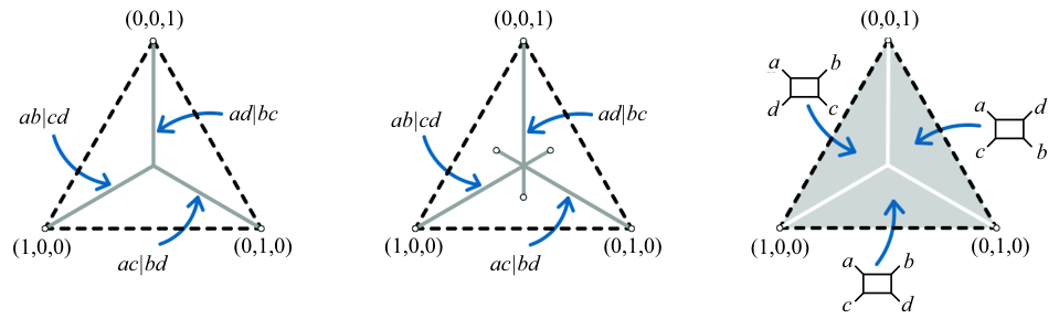
In Figure 4, we make concrete the proposition’s results. The CFs for binary quartet networks partition the simplex: $\Delta_{2}=\{\text{tree-like CFs}\}\sqcup\{4_{1}\text{-cycle CFs}\}$, with the collection of CFs for $3_{2}$-cycles meeting both subsets non-trivially. Notably, if a quartet network $N^{-}$ has no $3_{2}$-cycle, then CFs suffice to determine if $N^{-}_{c}$ is a tree or a 4-cycle. This idea underlies our algorithm, as well as the network identifiability results from [3].

Indeed, we see from the partition that (in the absence of $3_{2}$-cycles) the presence of 2-cycles and $3_{1}$-cycles has no impact on whether a quartet tree or 4-cycle network is supported. This observation leads to the non-identifiability of such cycles on a network by the proof method utilized in [3], and prevents NANUQ from detecting them too. However, since $2$- and $3_{1}$-cycles on a large network model ‘hybridization’ between the most closely related populations (two that split and then rejoin, or hybridization between two populations which have just split from a common one) the inability to infer that such hybridization events occurred by our method may not be too surprising. The SNaQ algorithm [1] is likewise unable to detect these, as it too is based on CFs.

Because concordance factors arising from quartet networks with a $3_{2}$-cycle (case 2 of Proposition 9) coincide with CFs for particular parameter choices for $4_{1}$-cycle networks and tree-like networks, such CFs must be handled with delicacy. Clearly, $3_{2}$-cycles on quartet networks are not identifiable from CFs, and therefore will not be reconstructed by the NANUQ algorithm which focuses only on 4-cycles and tree-like quartet networks. Because such $3_{2}$-cycles will be disregarded, we investigate them more fully next.

A first observation is that for a tree-like CF arising from a quartet network $N^{-}$ with a $3_{2}$-cycle, say with descendants $a$, $b$ of the hybrid node as in Figure 5, then $N^{-}_{c}$ has topology $ab|cd$. This is exactly the topology supported by the CF, when viewed as arising from a particular parameter choice on the $4$-taxon tree $ab|cd$. Thus, while determining if the CF arises from a $3_{2}$-cycle or a tree is not possible, a tree-like CF always correctly supports the topology of $N_{c}^{-}$.

This leaves the question of how ‘rare’ are non-tree-like $3_{2}$-cycle networks, and what metric structure on a $3_{2}$-cycle network might lead to CFs that coincide with $4_{1}$-cycle CFs.

Let $N^{-}$ be the unrooted quartet network shown in the left of Figure 5, with branch length parameters $t_{i}$ in coalescent units, and hybridization paramter $\gamma$ as shown. With $x_{i}=e^{-t_{i}}$ then [1, 3] the quartet concordance factors of $N^{-}$ are

We say a choice of parameters $\{t_{1},t_{2},t_{3},t_{4},\gamma\}$, or their transformed versions $x_{i}$, is tree-like if the CF for the network is tree-like for those parameters. The set of tree-like parameters for $N^{-}$ is a region in the 5-dimensional cube, $0\leq x_{1},x_{2},x_{3},x_{4},\gamma\leq 1,$ defined by the polynomial inequality $CF_{AB|CD}\geq CF_{AC|BD}.$

To get a sense of the size of the tree-like region on $N^{-}$, we sampled uniformly at random $10^{10}$ points in $[0,1]^{5}$. For untransformed branch length parameters $t_{i}$, this corresponds to sampling from an exponential distribution with mean 1. We computed that approximately $0.00532$ of the resulting CFs were not tree-like. In this sense, non-tree-like CFs from $3_{2}$-cycles are rare.

For additional insight into tree-like parameters on $N^{-}$, we investigate CFs as functions of $x_{1}$ and $x_{3}$, with $0<x_{2},x_{4},\gamma\leq 1$, noting that when $x_{2}$, $x_{4}$ achieve their maximum value of 1, this corresponds to the network with hybrid branch lengths $t_{2}=t_{4}=0$. Concretely, parameters are tree-like if

Hence parameters are tree-like for any values of $x_{2},x_{4},\gamma$ when $x_{1}\leq 4/(5-x_{3})$, a region shown in the center of Figure 5. This region has area $4\ln\frac{5}{4}\approx.89$. More crudely, provided $x_{1}\leq 4/5$ (that is, $t_{1}\geq\log(5/4)\approx 0.2231$ coalescent units), then a tree-like CF results regardless of all other parameter values. Thus non-tree-like parameters require that $t_{1}$ be fairly short, causing substantial incomplete lineage sorting. For comparison, if the internal branch on a rooted 3-taxon species tree has length $t<\log(5/4)$, then fewer than half of the gene trees match the species tree under the MSC.

Although this argument assumed the non-existence of $2_{1}$-, $2_{2}$-, and $3_{1}$-cycles in $N^{-}$, a general level-1 quartet network with a $3_{2}$-cycle might have cycles of those types. The result generalizes without difficulty to these more general networks, with $t_{1}$ the length of the edge descended from the $3_{2}$-hybrid node. For larger networks, we have the following proposition.

Before proving the proposition, note that an $m_{k}$-cycle in $N^{+}$ can induce not only a $4_{1}$-cycle in an induced quartet network, but also smaller cycles, depending on the particular choice of four taxa. For instance, a 4-cycle in the network of Figure 1 (L) leads to a $3_{2}$-cycle in the induced quartet network on $a,b,c,d$, as shown in Figure 2 (R).

The branch length hypotheses in Proposition 10 are sufficient, but not necessary, for tree-like CFs in the presence of $3_{2}$-cycles. For instance, if a tree edge $e$ descendant from a hybrid node in a $3_{2}$-cycle in $N^{+}$ is followed by one (or more) $2$-cycles, then the length requirement on $e$ to produce tree-like CFs might be shortened.

Focusing again on the quartet network of Figure 5, we now investigate transformed branch length parameters $x_{2}$, $x_{4}$ on hybrid edges that lead to tree-like parameter choices. To this end, let $M=\max(x_{2},x_{4})\leq 1$. Then from equation (1) for any $x_{3}$, $\gamma$, we find

and parameters are tree-like if $M\leq\min\left(\frac{2}{x_{1}}-\frac{3}{2},1\right)$, a region shown in blue in Figure 5 (R). Its area is $2\log(\frac{5}{4})+.5\approx 95\%$ of the $(x_{1},M)$-parameter space shown. As a special case, if $M\leq\frac{1}{2}$ (equivalently, $\min\{t_{2},t_{4}\}\geq\log(2)\approx 0.693$ coalescent units), parameters are tree-like for all choices of $(x_{1},x_{3},\gamma)$.

The branch length conditions presented here that rule out non-tree-like $3_{2}$-cycles come with a caution, since one might prefer to avoid a priori modeling assumptions on branch lengths. Nonetheless, our goal has been to suggest that plausible assumptions can rule out non-tree-like CFs arising from $3_{2}$-cycles in quartet networks. Inspection of empirical CFs from a data set may provide further evidence that no such CFs are involved in a data analaysis

We adopt standard terminology concerning splits [22]. A split $A|B=B|A$ of taxa $X$ is a bipartition $X=A\sqcup B$ with $A,B$ non-empty. The subsets $A$, $B$ are called split sets. The set of all splits of $X$ is denoted by $(X)$, and $\mathcal{S}\subseteq(X)$ is called a split system on $X$.

A circular ordering for ${\mathcal{S}}$ is not unique, since it can be modified by cyclically permuting the $x_{i}$ (e.g., replaced with $x_{2}<x_{3},<\dots<x_{n}<x_{1}$) or by inversion (replaced with $x_{n}<x_{n-1}<\dots<x_{1}$), while remaining a circular ordering for ${\mathcal{S}}$. We treat such variants as the same, without further comment.

Given a tree $T$ on $X$, deleting an edge defines a split according to the connected components of the resulting graph. The set of all such displayed splits is denoted $\mathcal{S}(T)$, and it is clear from a planar depiction of a tree that $\mathcal{S}(T)$ is circular.

For a tree, the correspondence between edges and displayed splits allows edge weights to be viewed as split weights, by setting weights of non-displayed splits to 0. This is a special case of a weighted split system on $X$, a map

A weighted split system $\omega$ on $X$ induces a distance function $d_{\omega}$ on $X$ by

where $S_{xy}\subseteq(X)$ is the set of splits separating $x$ and $y$, i.e., splits $A|B$, with $x\in A$ and $y\in B$. Clearly $d_{\omega}$ is non-negative valued, with $d_{\omega}(x,x)=0$, $d_{\omega}(x,y)=d_{\omega}(y,x)$.

Recall that the support of a weighted split system, denoted $\operatorname{supp}(\omega)$, is the set of splits on which $\omega$ is non-zero.

As pointed out in [22], it follows from [23] that a circular distance function $d$ uniquely determines the weighted split system $\omega$ such that $d=d_{\omega}$.

Our notion of splits associated to a network, and some related terminology, is not standard, but is essential to this work. In particular, we focus only on phylogenetic unrooted networks $N^{-}$ as in Definition 4, where $N^{-}$ is induced from a rooted phylogenetic network and the direction of hybrid edges are retained in $N^{-}$.

If $N^{-}$ has an $m$-cycle with $m\geq 4$, then the grove $\mathcal{G}(N^{-})$ is a proper subset of the displayed trees on the undirected network $N^{u}$ underlying $N^{-}$ as defined in [13]. This is because $N^{u}$ is obtained by undirecting the hybrid edges in $N^{-}$, and there is additional freedom in the choice of edges to delete in $N^{u}$ to obtain its displayed trees: It is not necessary to delete at least one of the edges from $N^{u}$ that arose from each pair of hybrid edges in $N^{-}$.

If $N^{-}$ has 2- or 3-cycles, then deleting either hybrid edge in those cycles yields trees with the same topology, and hence gives the same elements of $\mathcal{G}(N^{-})$. In contrast, for cycles of size 4 or larger, the trees in $\mathcal{G}(N^{-})$ vary with the choice of hybrid edge deleted. Since we assume that $N^{-}$ is level-1 with $k$ cycles of size $\geq 4$, then $|\mathcal{G}(N^{-})|=2^{k}$.

The study of undirected networks in [13] provides the following important theorem, an analog for undirected networks of Buneman’s splits equivalence theorem.

Note that if $N^{u}$ is the undirected network underlying the unrooted network $N^{-}$, then ${\mathcal{S}}(N^{-})\subseteq{\mathcal{S}}(N^{u})$. As a consequence, we obtain the following.

For an unrooted binary topological phylogenetic tree $T$ on $X$, any internal edge $e$ induces a partition of $X$ into 4 non-empty blocks, $X_{1}$, $X_{2}$, $X_{3}$ and $X_{4}$, where the split associated to $e$ is $s_{e}=X_{1}\cup X_{2}|X_{3}\cup X_{4}$, and the splits associated to the 4 adjacent edges have an $X_{i}$ as one split set. Similarly, a pendant edge $e$ to taxon $a$ induces a partition into 3 blocks $X_{1}$, $X_{2}$ and $\{a\}$, where $s_{e}=\{a\}|X_{1}\cup X_{2}$, and the splits associated to the 2 edges adjacent to $e$ have an $X_{i}$ as one split set. The quartet weight function $w_{T}:(X)\to{\mathbb{R}}$ is defined as

This split weight function then induces $d_{w_{T}}$, the quartet distance function on $X$. This distance is a tree metric, and therefore can be used to reconstruct the topological binary $n$-taxon tree $T$ by several algorithms. Significantly, the distance function $d_{w_{T}}$ can computed another way, from the set of quartets displayed on $T$, without prior knowledge of the full tree topology.

To generalize Theorem 17 to a network, we begin with a definition.

Note that since $\operatorname{supp}(w_{T})=\mathcal{S}(T)$ for each $T$, $\operatorname{supp}(\omega_{N^{-}})=S(N^{-})$. Thus, by Corollary 16, the quartet weight function $\omega_{N^{-}}$ is a weighted circular split system for $N^{-}$. Moreover, the induced distance function is easily related to those for the trees in the grove $\mathcal{G}(N^{-})$.

To state a network analog of Theorem 17, we must extend the indicator function $\rho_{xy}$ to quartet networks.

In the case $Q_{xyzw}$ is a tree, this definition agrees with that in Theorem 17. An intuitive way of viewing this extension to networks is to observe that when $\widetilde{Q}_{xyzw}$ is a 4-cycle, $\rho_{xy}(Q_{xyzw})$ is the average of the values of $\rho_{xy}(T)$ for $T\in\mathcal{G}(\widetilde{Q}_{xyzw})$, so $\rho_{xy}$ measures how separated $x$ and $y$ are on $Q_{xyzw}$. See Figure 6.

We now define a distance function in terms of quartet networks displayed on the network.

Note that if $N^{-}=T$ is a tree, the definition of $d_{Q,N^{-}}(x,y)$ agrees with equation (2). We now prove the network analog of Theorem 17, showing that the network distance $d_{\omega_{N^{-}}}$ can be computed from induced quartet networks.

The import of this theorem is that from the induced quartet networks on $N^{-}$ we can compute the distance $d_{Q,N^{-}}$, which is, up to scaling, $d_{\omega_{N^{-}}}$, the distance from a weighted split system. In contrast, computing $d_{\omega_{N^{-}}}$ directly from definition requires knowing $\mathcal{G}(N^{-})$, the collection of trees on $X$ displayed on $N^{-}$. This lies at the heart of our algorithm for network inference under the NMSC, as we can obtain information about induced quartet networks from biological data relatively easily, using empirical concordance factors, while information about the trees displayed on the species network does not seem to be directly obtainable.

Furthermore, since by Corollary 16 the underlying quartet weighted split system is circular, we have the following.

Thus given sufficient information on induced quartet networks to compute $d_{Q,N^{-}}$, even approximately as in the presence of error, methods for analyzing distances from weighted circular split systems, such as the NeighborNet algorithm, can be productively applied, as we show in the next section.

References

- [1] Solís-Lemus, C., Ané, C.: Inferring phylogenetic networks with maximum pseudolikelihood under incomplete lineage sorting. PLoS Genetics 12(3) (2016). doi:10.1371/journal.pgen.1005896
- [2] Yu, Y., Nakhleh, L.: A maximum pseudo-likelihood approach for phylogenetic networks. BMC Genomics 16, 10 (2015). Chap. S10
- [3] Baños, H.: Identifying species network features from gene tree quartets. Bulletin of Mathematical Biology 81, 494–534 (2019)
- [4] Allman, E.S., Mitchell, J.D., Rhodes, J.A.: Hypothesis testing near singularities and boundaries. https://arxiv.org/abs/1806.08458 (2018)
- [5] Rhodes, J.A.: Topological metrizations of trees, and new quartet methods of tree inference. IEEE/ACM Transactions on Computational Biology and Bioinformatics (2019, to appear)
- [6] Bryant, D., Moulton, V.: Neighbor-Net: An agglomerative method for the construction of phylogenetic networks. Molecular Biology and Evolution 21, 255–265 (2004)
- [7] Dress, A.W.M., Huson, D.H.: Constructing splits graphs. IEEE/ACM Transactions on Computational Biology and Bioinformatics 1(3), 109–115 (2004). doi:10.1109/TCBB.2004.27
- [8] Huson, D.H., Bryant, D.: Application of phylogenetic networks in evolutionary studies. Molecular Biology and Evolution 23(2), 254–267 (2005). doi:10.1093/molbev/msj030
- [9] Wen, D., Nakhleh, L.: Coestimating reticulate phylogenies and gene trees from multilocus sequence data. Systematic Biology 67(3), 439–457 (2018)
- [10] Zhang, C., Ogilvie, H.A., Drummond, A.J., Stadler, T.: Bayesian inference of species networks from multilocus sequence data. Mol. Biol. Evol. 35(2), 504–517 (2018)
- [11] Huson, D.H., Rupp, R., Scornavacca, C.: Phylogenetic Networks. Cambridge University Press, Cambridge (2010)
- [12] Huson, D.H., Klöpper, T., Lockhart, P.J., Steel, M.A.: Reconstruction of reticulate networks from gene trees. In: Miyano, S., Mesirov, J., Kasif, S., Istrail, S., Pevzner, P.A., Waterman, M. (eds.) Research in Computational Molecular Biology. RECOMB 2005. Lecture Notes in Computer Science, vol. 3500. Springer, Berlin, Heidelberg (2005)
- [13] Gambette, P., Berry, V., Paul, C.: Quartets and unrooted phylogenetic networks. Journal of Bioinformatics and Computational Biology 10(4), 1250004 (2012). doi:10.1142/S0219720012500047
- [14] Steel, M.: Phylogeny: Discrete and Random Processes in Evolution. CBMS-NSF Regional Conference Series in Applied Mathematics, vol. 89. Society for Industrial and Applied Mathematics (SIAM), Philadelphia, PA (2016). doi:10.1137/1.9781611974485.ch1
- [15] Rosselló, F., Valiente, G.: All that glisters is not galled. Mathematical Biosciences 221(1), 54–59 (2009). doi:10.1016/j.mbs.2009.06.007
- [16] Pamilo, P., Nei, M.: Relationships between gene trees and species trees. Mol. Biol. Evol. 5(5), 568–583 (1988)
- [17] Liu, L., Yu, L., Kubatko, L., Pearl, D.K., Edwards, S.V.: Coalescent methods for estimating phylogenetic trees. Mol. Phylogenet. Evol. 53(1), 320–328 (2009)
- [18] Meng, C., Kubatko, L.S.: Detecting hybrid speciation in the presence of incomplete lineage sorting using gene tree incongruence: A model. Theoretical Population Biology 75(1), 35–45 (2009). doi:10.1016/j.tpb.2008.10.004
- [19] Yu, Y., Degnan, J.H., Nakhleh, L.: The probability of a gene tree topology within a phylogenetic network with applications to hybridization detection. PLoS Genetics 8, 1002660 (2012)
- [20] Zhu, J., Yu, Y., Nakhleh, L.: In the light of deep coalescence: Revisiting trees within networks. BMC Bioinformatics 17, 415 (2016). Chap. 415
- [21] Allman, E.S., Degnan, J.H., Rhodes, J.A.: Identifying the rooted species tree from the distribution of unrooted gene trees under the coalescent. Journal of Mathematical Biology 62(6), 833–862 (2011). doi:10.1007/s00285-010-0355-7. 0912.4472
- [22] Bryant, D., Moulton, V., Spillner, A.: Consistency of the Neighbor-Net algorithm. Algorithms for Molecular Biology 2:8 (2007)
- [23] Bandelt, H., Dress, A.: A canonical decomposition theory for metrics on a finite set. Advances in Mathematics 92, 47–105 (1992)
- [24] Dress, A., Moulton, V., Terhalle, W.: -theory: an overview. European J. Combin. 17(2-3), 161–175 (1996). doi:10.1006/eujc.1996.0015. Discrete metric spaces (Bielefeld, 1994)
- [25] Chifman, J., Kubatko, L.: An invariants-based method for efficient identification of hybrid species from large-scale genomic data. BMC Evolutionary Biology (2019, to appear)
- [26] Allman, E.S., Long, C., Rhodes, J.A.: Species tree inference from genomic sequences using the log-det distance. SIAM J. Appl. Algebra Geom. 3(1), 107–127 (2019). doi:10.1137/18M1194134
- [27] Roch, S., Wang, K.-C.: In: Raphael, B. (ed.) Circular Networks from Distorted Metrics. Lecture Notes in Computer Science, vol. 10812. Springer, New York (2018)
- [28] Rokas, A., Williams, B., Carrol, S.: Genome-scale approaches to resolving incongruence in molecular phylogenies. Nature 425, 798–804 (2003)
- [29] Martin, S.H., K.K., D., Nadeau, N.J., Salazar, C., Walters, J.R., Simpson, F., Blaxter, M., Manica, A., Mallet, J., Jiggins, C.D.: Genome-wide evidence for speciation with gene flow in Heliconius butterflies. Genome Res 23, 1817–1828 (2013)
- [30] Zhu, S., Degnan, J.H., Goldstien, S., Eldon, B.: Hybrid-Lambda: Simulation of multiple merger and Kingman gene genealogies in species networks and species trees. BMC Bioinformatics 16(1), 292 (2015). doi:10.1186/s12859-015-0721-y
- [31] Bloomquist, D., Suchard, M.: Unifying vertical and nonvertical evolution: A stochastic arg-based framework. Systematic Biology 59, 27–41 (2010)
- [32] Holland, B.R., Huber, K.T., Moulton, V., Lockhart, P.J.: Using consensus networks to visualize contradictory evidence for species phylogeny. Molecular Biology and Evolution 21(7), 1459–1461 (2004). doi:10.1093/molbev/msh145
- [33] Wu, Q., James, S., Roberts, I., Moulton, V., Huber, K.: Exploring contradictory phylogenetic relationships in yeasts. FEMS Yeast Research 8, 641–650 (2008)
- [34] Yu, Y., Than, C., Degnan, J.H., Nakhleh, L.: Coalescent histories on phylogenetic networks and detection of hybridization despite incomplete lineage sorting. Systematic Biology 60(2), 138–149 (2011). doi:10.1093/sysbio/syq084