On the spherical quasi-convexity of quadratic functions
on spherical self-dual convex sets

O. P. Ferreira Thanks: IME/UFG, Avenida Esperança, s/n, Campus II, Goiânia, GO - 74690-900, Brazil (E-mails: orizon@ufg.br). S. Z. Németh Thanks: School of Mathematics, University of Birmingham, Watson Building, Edgbaston, Birmingham - B15 2TT, United Kingdom (E-mail: s.nemeth@bham.ac.uk, LXX490@student.bham.ac.uk). L. Xiao ³³footnotemark: 3

Abstract

In this paper, the spherical quasi-convexity of quadratic functions on spherically subdual convex sets is studied. Sufficient conditions for spherical quasi-convexity on spherically subdual convex sets are presented. A partial characterization of spherical quasi-convexity on spherical Lorentz sets is given and some examples are provided.

Keywords: Spherical quasi-convexity, quadratic function, self-dual cone.
AMS subject classification:. 26B25 $\cdot$ 90C25

1 Introduction

The aim of this paper is to study theoretical properties of spherical quasi-convexity of quadratic functions on spherically subdual convex sets. It is well known that quadratic functions play an important role in nonlinear programming theory. For instance, the minimization problem of quadratic functions on the sphere occurs as a subproblem in methods of nonlinear programming (see the background section of [1] for an extensive review of the literature on the subject). We are interested in the problem of minimizing a quadratic function, defined by the symmetric matrix $Q$ , constrained to a subset $C$ of the sphere. This problem is a quadratic constrained optimization problem on the sphere, and it is also a minimum eigenvalue problem in $C$ . It is essential to emphasize that there exists a special case, when $C$ is the intersection of the Lorentz cone with the sphere. This special case is of particular interest because the minimum eigenvalue of $Q$ in $C$ is non-negative, if and only if the matrix $Q$ is Lorentz copositive; see [2, 3]. In general, changing the Lorentz cone by an arbitrary closed and convex cone $K$ would lead to a more general concept of $K$ -copositivity, thus our study is anticipated to initialize new perspectives for investigating the general copositivity of a symmetric matrix. In general, exploiting the specific intrinsic geometric and algebraic structure of problems posed on the sphere can significantly lower down the cost of finding solutions; see [4, 5, 6, 7, 8, 9]. We know that a strict local minimizer of a spherically quasi-convex quadratic function is also a strict global minimizer, which makes interesting and natural to refer the problem about characterizing the spherically quasi-convex quadratic functions on spherically convex sets.

The aim of this paper is to introduce both sufficient conditions and necessary conditions for quadratic functions to be spherically quasi-convex on spherically subdual convex sets. In particular, several examples are presented. This paper continues the study of [10], which can be regarded as premier study about the topic of quasi-convexity of quadratic functions on the Euclidean space. The main literature about the quasi-convexity of quadratic functions on Euclidean convex sets includes, but it is not limited to [11, 12, 13, 14, 15].

The remaining part of this paper is structured as follows. Section 2 presents previous results and notations, that will be used throughout this paper. In Section 2.1, we recall the fundamental properties of spherically quasi-convex functions on spherically convex sets and, in Section 2.1.1, particular versions of these conditions for quadratic spherically quasi-convex functions. Section 3 provides derivations of many useful properties of spherically quasi-convex functions on spherically subdual convex sets. In Section 4, we prove a condition partially characterizing the spherical quasi-convexity of quadratic functions on spherically convex sets associated with the Lorentz cone. Perspectives and open problems are presented in Section 5 and Section 6 concludes the paper.

2 Terminology and Basics Results

In this section, we introduce some notations and present the previous results used throughout the paper. Let $\mathbb{R}^{n}$ be the $n$ -dimensional Euclidean space with the canonical inner product $\langle\cdot,\cdot\rangle$ and norm $\|\cdot\|$ . For a set $D\subset\mathbb{R}^{n}$ , denote by $[D]$ the span of a set $D$ , i.e., the smallest linear subspace of $\mathbb{R}^{n}$ that contains the set $D$ . For a vector subspace $\mathbb{V}\subset\mathbb{R}^{n}$ , denote by $\mathbb{V}^{\perp}=\{x\in\mathbb{R}^{n}:~\langle v,x\rangle=0,~\forall~v\in\mathbb{V}\}$ its orthogonal complement in $\mathbb{R}^{n}$ . In particular, for simplifying the notation, for a vector $u\in\mathbb{R}^{n}$ we set $[u]:=[\{u\}]$ and $[u]^{\perp}:=[\{u\}]^{\perp}$ . Denote by $\mathbb{R}^{m\times n}$ the set of all $m\times n$ matrices with real entries, $\mathbb{R}^{n}\equiv\mathbb{R}^{n\times 1}$ , by $e^{i}$ the $i$ -th canonical unit vector in $\mathbb{R}^{n}$ , and by ${\rm I_{n}}$ the $n\times n$ identity matrix. A set ${\cal K}\subseteq\mathbb{R}^{n}$ is called a cone if for any $\alpha>0$ and $x\in\cal{K}$ we have $\alpha x\in\cal{K}$ . A cone ${\cal K}\subseteq\mathbb{R}^{n}$ is called a convex cone if for any $x,y\in\cal{K}$ , we have $x+y\in\cal{K}$ . The dual cone of a cone ${\cal{K}}\subseteq\mathbb{R}^{n}$ is the closed convex cone ${\cal{K}}^{*}\!\!:=\!\{x\in\mathbb{R}^{n}:~\langle x,y\rangle\!\geq\!0,~\forall\,y\!\in\!{\cal{K}}\}.$ A cone ${\cal K}\subseteq\mathbb{R}^{n}$ is called pointed if ${\cal K}\cap{(-\cal K)}\subseteq\{0\}$ . A pointed closed convex cone is called proper cone if it has a nonempty interior. The cone ${\cal K}\subseteq\mathbb{R}^{n}$ is called subdual if ${\cal K}\subseteq{\cal K}^{*}$ and self-dual if ${\cal K}={\cal K}^{*}$ . The Lorentz cone is defined by

{\cal L}:=\left\{x=(x_{1},\dots,x_{n})^{\top}\in\mathbb{R}^{n}:~x_{1}\geq\sqrt{(x_{2})^{2}+\dots+(x_{n})^{2}}\right\},

which is a special case of the elliptic cone defined by

{\cal E}:=\left\{x\in\mathbb{R}^{n}:~\langle v^{1},x\rangle\geq\sqrt{\theta_{2}\langle v^{2},x\rangle^{2}+\dots+\theta_{n}\langle v^{n},x\rangle^{2}}\right\},

where $\theta_{2},\ldots,\theta_{n}$ are positive real numbers and $v^{1},v^{2},\ldots,v^{n}$ are L.I. vectors in $\mathbb{R}^{n}$ . We recall that the Lorentz cone ${\cal L}$ and the non-negative orthant $\mathbb{R}^{n}_{+}$ are self-dual cones. Let ${\cal K}$ be a closed convex cone. Let $x\in\mathbb{R}^{n}$ , then the projection $P_{\cal K}(x)$ of the point $x$ onto the cone ${\cal K}$ is defined by

P_{\cal K}(x):=\operatorname{argmin}\left\{\|x-y\|~:~y\in{\cal K}\right\}.

For any $x\in{\cal K}$ , we define the non-negative part of $x$ , nonpositive part of $x$ and the absolute value of $x$ with respect to ${\cal K}$ by

x_{+}^{\cal K}:={\rm P}_{\cal K}(x),\qquad x_{-}^{\cal K}:={\rm P}_{{\cal K}^{*}}(-x),\qquad|x|^{\cal K}:=x_{+}^{\cal K}+x_{-}^{\cal K},

(1)

respectively. We recall from Moreau’s decomposition theorem [16] (see also [17, Theorem 3.2.5]), that for a closed convex cone ${\cal K}$ there hold:

x=x_{+}^{\cal K}-x_{-}^{\cal K},\qquad\left\langle x_{+}^{\cal K},x_{-}^{\cal K}\right\rangle=0,\qquad\qquad~x\in\mathbb{R}^{n}.

(2)

For any $z\in\mathbb{R}\times{\mathbb{R}}^{n-1}$ , let $z:=(z_{1},{z^{2}})\in\mathbb{R}\times{\mathbb{R}}^{n-1}$ , where ${z^{2}}:=(z_{2},z_{3},\dots,z_{n})^{{}^{\top}}$ . An explicit formula for the projection mapping ${\rm P}_{\cal{L}}$ onto the Lorentz cone ${\cal L}$ is given in [18, Proposition 3.3], which is recalled for the case when $x\notin{\cal L}\cup-{\cal L}$ in the following lemma.

Lemma 1.

Let $x=(x_{1},{x^{2}})\in\{(y_{1},{y^{2}})\in\mathbb{R}\times\mathbb{R}^{n-1}:~|y_{1}|<\|{y^{2}}\|\}$ and ${\cal{L}}$ be the Lorentz cone. Then,

x_{+}^{\cal L}=\left(\frac{x_{1}+\|{x^{2}}\|}{2\|x^{2}\|}\right)\left(\|x^{2}\|,x^{2}\right),\qquad x_{-}^{\cal L}=\left(\frac{-x_{1}+\|{x^{2}}\|}{2\|x^{2}\|}\right)\left(\|x^{2}\|,-x^{2}\right)

and, as a consequence, the absolute value of $x$ with respect to ${\cal L}$ is given by

|x|^{\cal L}=\frac{1}{\|x^{2}\|}\left(\|{x^{2}}\|^{2},x_{1}x^{2}\right).

For a general nonzero vector $x=\left(x_{1},{x^{2}}\right)\in\mathbb{R}\times\mathbb{R}^{n-1}$ the absolute value of $x$ with respect to ${\cal L}$ is given in the next lemma, which follows immediately from Lemma 1 and equations (2).

Lemma 2.

Consider a nonzero vector $x=\left(x_{1},{x^{2}}\right)\in\mathbb{R}\times\mathbb{R}^{n-1}$ and let ${\cal{L}}$ be the Lorentz cone. Then, the absolute value of $x$ is given by

|x|^{\cal L}=\frac{1}{\|x^{2}\|}\Big(\operatorname{max}\left(|x_{1}|,\|{x^{2}}\|\right)\|x^{2}\|,~\operatorname{min}(|x_{1}|,\|x^{2}\|)\sgn(x_{1})x^{2}\Big),

where $\sgn(x_{1})$ is equal to $-1$ , $0$ or $1$ whenever $x_{1}$ is negative, zero or positive, respectively.

Let ${\cal K}\subseteq\mathbb{R}^{n}$ be a (not necessarily convex) cone. Let us recall that $A\in\mathbb{R}^{n\times n}$ is ${\cal K}$ -copositive if $\langle Ax,x\rangle\!\geq\!0$ for all $x\in{\cal K}$ and a Z-matrix is a matrix with nonpositive off-diagonal elements. It is easy to see that the Lorentz cone ${\cal{L}}$ can be written as

{\cal L}:=\left\{x=(x_{1},\dots,x_{n})^{\top}\in\mathbb{R}^{n}:~x_{1}\geq 0,\textrm{ }\langle Jx,x\rangle\geq 0\right\},

where $J=\diag(1,-1,\dots,-1)\in\mathbb{R}^{n\times n}$ . It is easy to see that

{\cal L}\cup-{\cal L}=\left\{x=(x_{1},\dots,x_{n})^{\top}\in\mathbb{R}^{n}:\langle Jx,x\rangle\geq 0\right\}.

This straightforwardly implies that $A\in\mathbb{R}^{n\times n}$ is ${\cal L}$ -copositive if and only if it is ${\cal L}\cup-{\cal L}$ -copositive. Hence, the S-Lemma (see [19, 20, 21]) implies:

Lemma 3.

$A\in\mathbb{R}^{n\times n}$ is ${\cal L}$ -copositive if and only if there exists a $\rho\geq 0$ such that $A-\rho J$ is positive semidefinite.

This result is well-known and it is remarked in Lemma 2.2 of [2]. Let ${\cal K}\subseteq\mathbb{R}^{n}$ be a pointed closed convex cone with nonempty interior, the ${\cal K}$ -Z-property of a matrix $A\in\mathbb{R}^{n\times n}$ means that $\langle Ax,y\rangle\leq 0$ , for any $(x,y)\in C({\cal K})$ , where $C({\cal K}):=\{(x,y)\in\mathbb{R}^{n}\times\mathbb{R}^{n}:~x\in{\cal K},\textrm{ }y\in{\cal K}^{*},\langle x,y\rangle=0\}$ . Throughout the paper the $n$ -dimensional Euclidean sphere $\mathbb{S}^{n-1}$ is denoted by

\mathbb{S}^{n-1}:=\left\{x=(x_{1},\ldots,x_{n})^{\top}\in\mathbb{R}^{n}~:~\|x\|=1\right\}.

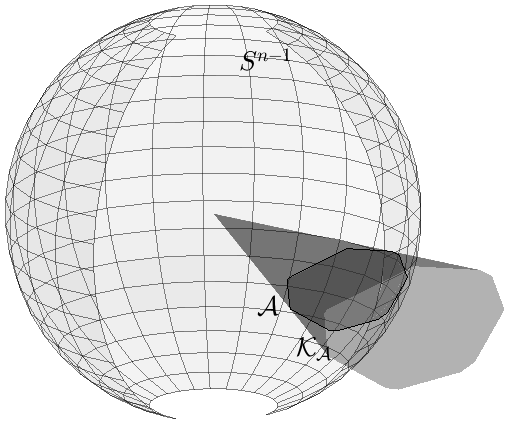
The intrinsic distance on the sphere between $x,y\in\mathbb{S}^{n-1}$ is defined by $\dist(x,y):=\arccos\langle x,y\rangle.$ It is also easy to verify that $\dist(x,y)\leq\pi$ for any $x,y\in\mathbb{S}^{n-1}$ , and $\dist(x,y)=\pi$ if and only if $x=-y$ . The intersection curve of a plane through the origin of $\mathbb{R}^{n}$ with the sphere $\mathbb{S}^{n-1}$ is called a geodesic. A geodesic segment joining $x$ to $y$ is said to be minimal if its length is equal to $\dist(x,y)$ . A set ${\cal C}\subseteq\mathbb{S}^{n-1}$ is said to be spherically convex if for any $x$ , $y\in{\cal C}$ all the minimal geodesic segments joining $x$ to $y$ are contained in ${\cal C}$ . For notational convenience, in the following text we assume that all spherically convex sets are nonempty proper subsets of the sphere. For each closed set ${\cal A}\subseteq\mathbb{S}^{n-1}$ , let ${\cal K}_{\cal A}\subseteq\mathbb{R}^{n}$ be the cone spanned by ${\cal A}$ , namely,

{\cal K}_{\cal A}\>=\left\{tx\,:\,x\in{\cal A},\;t\in[0,+\infty)\right\}.

Refer to caption — Figure 1: Closed set ${\cal A}$ and the cone ${\cal K}_{\cal A}$ spanned by ${\cal A}$ .

Obviously, ${\cal K}_{\cal A}$ is the smallest cone containing ${\cal A}$ (see Fig. 1). In the following proposition, a relationship between spherically convex sets and the cones spanned by them will be exhibited. The proof is given in [22, Proposition 2].

Proposition 1.

The set ${\cal C}$ is spherically convex if and only if the cone $\mathcal{K}_{\cal C}$ is pointed convex.

2.1 Spherically quasi-convex functions on spherically convex sets

In this section we recall the concept of spherically quasi-convex functions on spherically convex sets and we present a basic characterization of them; for more details see [10].

Definition 1.

Let ${\cal C}\subseteq\mathbb{S}^{n-1}$ be a spherically convex set and $I\subseteq\mathbb{R}$ be an interval. A function $f:{\cal C}\to\mathbb{R}$ is said to be spherically quasi-convex (respectively, strictly spherically quasi-convex) if for any minimal geodesic segment $\gamma:I\to{\cal C}$ , the composition $f\circ\gamma:I\to\mathbb{R}$ is quasi-convex (respectively, strictly quasi-convex) in the usual sense, i.e., $f(\gamma(t))\leq\operatorname{max}\{f(\gamma(t_{1})),f(\gamma(t_{2}))\}$ for all $t\in[t_{1},t_{2}]\subseteq I$ , (respectively, $f(\gamma(t))<\operatorname{max}\{f(\gamma(t_{1})),f(\gamma(t_{2}))\}$ for all $t\in[t_{1},t_{2}]\subseteq I$ , $t_{1}\neq t_{2}$ ).

Remark 1.

The above definition implies that, if $f:\mathbb{S}^{n-1}\to\mathbb{R}$ is spherically quasi-convex, then $f$ is constant. However, as wee will show, there exist non-constant spherically quasi-convex functions defined on proper convex sets of $\mathbb{S}^{n-1}$ .

To simplify the notations, the sub-level sets of a function $f:\mathbb{R}^{n}\supseteq{\cal M}\to\mathbb{R}$ are denoted by

[f\leq c]:=\{x\in{\cal M}:\;f(x)\leq c\},\qquad c\in\mathbb{R}.

Proposition 2.

Let ${\cal C}\subseteq\mathbb{S}^{n-1}$ be a spherically convex set. A function $f:{\cal C}\to\mathbb{R}$ is spherically quasi-convex if and only if for all $c\in\mathbb{R}$ the sub-level sets $[f\leq c]$ are spherically convex.

2.1.1 Spherically quasi-convex quadratic functions on spherically convex sets

In this section we recall earlier results of quadratic quasi-convex functions on general spherically convex sets. Henceforward we assume that the cone ${\cal K}\subseteq\mathbb{R}^{n}$ is proper and subdual, the set ${\cal C}=\mathbb{S}^{n-1}\cap\inte({\cal K})$ is open and spherically convex, and $A=A^{T}\in\mathbb{R}^{n\times n}$ . Let $q_{A}:{\cal C}\to\mathbb{R}$ be the quadratic function defined by

q_{A}(x):=\langle Ax,x\rangle.

(3)

To proceed we need as well the restriction on $\inte{\cal K}$ of Rayleigh quotient $\varphi_{A}:\inte{\cal K}\to\mathbb{R}$ defined by

\varphi_{A}(x):=\frac{\langle Ax,x\rangle}{\|x\|^{2}}.

(4)

In the followings we state some properties of the functions $q_{A}$ and $\varphi_{A}(x)$ , for details see [10].

Proposition 3.

The following statements are equivalent:

(a)

$q_{A}$ is spherically quasi-convex;
(b)

$\langle Ax,y\rangle\leq\langle x,y\rangle\operatorname{max}\left\{q_{A}(x),~q_{A}(y)\right\}$ , for all $x,y\in\mathbb{S}^{n-1}\cap{\cal K}$ ;
(c)

$\displaystyle\frac{\langle Ax,y\rangle}{\langle x,y\rangle}\leq\operatorname{max}\left\{\varphi_{A}(x),~\varphi_{A}(y)\right\}$ , for all $x,y\in{\cal K}$ with $\langle x,y\rangle\neq 0$ .

Corollary 1.

Let ${\cal K}$ be self-dual. If $q_{A}$ is spherically quasi-convex, then $A$ has the $\cal K$ -Z-property.

Theorem 1.

The function $q_{A}$ is spherically quasi-convex if and only if $\varphi_{A}$ is quasi-convex.

The next result uses the following notations: Let $c\in\mathbb{R}$ and define the cone

[\varphi_{A}\leq c]:=\{x\in{\cal K}:\langle A_{c}x,x\rangle\leq 0\},\qquad A_{c}:=A-c{\rm I_{n}}.

Corollary 2.

The function $q_{A}$ is spherically quasi-convex if and only if $[\varphi_{A}\leq c]$ is convex, for any $c\in\mathbb{R}$ .

3 Spherically Quasi-Convex Quadratic Functions on Spherically Subdual Convex Sets

In this section we present partial conditions characterizing the spherical quasi-convexity of quadratic functions on spherically subdual convex sets associated to subdual cones. The results obtained generalize the corresponding ones obtained in [10, Section 4.1]. In due course we will present a more precise correspondence. Throughout this section we assume that ${\cal K}$ is subdual, i.e., ${\cal K}\subseteq{\cal K}^{*}$ and proper. A closed set ${\cal A}\subseteq\mathbb{S}^{n-1}$ is called spherically subdual convex set if the associated cone ${\cal K}_{\cal A}$ is subdual. It is clear that if $A=A^{\top}\in\mathbb{R}^{n\times n}$ has only one eigenvalue, then $q_{A}$ is constant and, consequently, it is spherically quasi-convex. Henceforth, throughout this section we assume that $A$ has at least two distinct eigenvalues. Let us recall that $q_{A}$ and $\varphi_{A}$ are defined in (3) and (4), respectively. Two technical lemmas, which are useful in the following text, will be presented. They are generalizations of Lemmas 14 and 15 of [10], respectively. More specifically, in Lemma 14 of [10] a condition implying the convexity of $[\varphi_{A}\leq c]$ , for all $c\notin(\lambda_{2},\lambda_{n})$ , is presented if $K={\mathbb{R}}^{n}_{+}$ , while here in Lemma 4 that condition is extended to an arbitrary subdual cone. Similarly, Lemma 6 generalizes Lemma 15 of [10] from $K={\mathbb{R}}^{n}_{+}$ to an arbitrary subdual cone. For stating the next lemma, for $\{v^{1},v^{2},\dots,v^{n}\}$ a orthonormal system of eigenvectors of $A$ corresponding to the eigenvalues $\lambda_{1}<\lambda_{2}\leq\ldots\leq\lambda_{n}$ , respectively, and $c\in(\lambda_{1},\lambda_{2}]$ , define the convex cone

{\cal L}_{c}:=\left\{x\in\mathbb{R}^{n}:~\langle v^{1},x\rangle\geq\sqrt{\theta_{2}(c)\langle v^{2},x\rangle^{2}+\dots+\theta_{n}(c)\langle v^{n},x\rangle^{2}}\right\},\qquad\theta_{i}(c):=\frac{\lambda_{i}-c}{c-\lambda_{1}},

(5)

for $i=2,\ldots,n$ . Note that if $\lambda_{1}<c<\lambda_{2}$ , then $\theta_{i}(c)>0$ , for $i=2,\ldots,n$ , and $\mathcal{L}_{c}$ , $-\mathcal{L}_{c}$ are also a pointed proper elliptic cones. We also need to consider the following cone

{\mathcal{W}}:=(\mathcal{L}_{\lambda_{2}}\cup-\mathcal{L}_{\lambda_{2}})\cap\inte({\mathcal{K}}).

(6)

Considering that ${\mathcal{K}}$ is a proper cone, then the cone ${\mathcal{W}}$ is also proper, i.e., $\inte({\mathcal{W}})\neq\varnothing$ .

Lemma 4.

Let $n\geq 2$ , $A=A^{\top}\in\mathbb{R}^{n\times n}$ and $\{v^{1},v^{2},\dots,v^{n}\}$ be an orthonormal system of eigenvectors of $A$ corresponding to the eigenvalues $\lambda_{1}<\lambda_{2}\leq\ldots\leq\lambda_{n}$ , respectively. Then, the sublevel set $[\varphi_{A}\leq c]$ is convex for all $c\notin(\lambda_{2},\lambda_{n})$ if and only if $v^{1}\in{\cal W}^{*}\cup-{\cal W}^{*}$ . In particular if $v^{1}\in{\cal K}^{*}$ , then $[\varphi_{A}\leq c]$ is convex for all $c\notin(\lambda_{2},\lambda_{n})$ .

Proof.

By using the spectral decomposition of $A$ , we have $A=\sum_{i=1}^{n}\lambda_{i}v^{i}(v^{i})^{\top}$ . From (4) we have

[\varphi_{A}\leq c]=\Big\{x\in\inte({\cal K}):~\sum_{i=1}^{n}(\lambda_{i}-c)\langle v^{i},x\rangle^{2}\leq 0\Big\}.

(7)

If $\lambda_{1}<c\leq\lambda_{2}$ , then by using (5) the equality (7) can be completed as follows

	$\displaystyle{\mathcal{W}}=[\varphi_{A}\leq\lambda_{2}]\supseteq[\varphi_{A}\leq c]$	$\displaystyle=({\mathcal{L}}_{c}\cup-{\mathcal{L}}_{c})\cap\inte({\mathcal{K}})$
		$\displaystyle=\left\{x\in\inte(\mathcal{K}):~\langle v^{1},x\rangle^{2}\geq\theta_{2}(c)\langle v^{2},x\rangle^{2}+\dots+\theta_{n}(c)\langle v^{n},x\rangle^{2}\right\}.$		(8)

Sufficiency of the first statement: Let $v^{1}\in{\cal W}^{*}$ (a similar argument holds for $v^{1}\in-{\cal W}^{*}$ ). If $c<\lambda_{1}$ , then considering that $v^{1},v^{2},\ldots,v^{n}$ are linearly independent and $0\notin\inte({\cal K})$ , we obtain from (7) that $[\varphi_{A}\leq c]=\varnothing$ and hence it is convex. If $c=\lambda_{1}$ , then (7) implies that $[\varphi_{A}\leq c]={\cal S}\cap\inte({\cal K}),$ where ${\cal S}:=\{x\in\mathbb{R}^{n}~:\langle v^{i},x\rangle=0,~\mbox{for}~i=2,\ldots,n\}$ . Thus, due to $\inte({\cal K})$ and ${\cal S}$ being convex, we conclude that $[\varphi_{A}\leq c]$ is also convex. Now, we suppose that $\lambda_{1}<c\leq\lambda_{2}$ . Since $v^{1}\in{\cal W}^{*}$ , for any $x\in\mathcal{W}$ we obtain that $\langle v^{1},x\rangle\geq 0$ and from (3) we have $[\varphi_{A}\leq c]={\cal L}_{c}\cap\inte({\cal K})$ . Due to the convexity of the cones ${\cal L}_{c}$ and $\inte({\cal K})$ , we obtain that $[\varphi_{A}\leq c]$ is convex. Finally, if $c\geq\lambda_{n}$ , then (7) implies that $[\varphi_{A}\leq c]=\inte({\cal K})$ is convex.
Necessity of the first statement: We will show that $v^{1}\notin{\cal W}^{*}\cup-{\cal W}^{*}$ implies that $[\varphi_{A}\leq c]$ is not convex, for some $c\in(\lambda_{1},\lambda_{2})$ . Suppose that $v^{1}\notin{\cal W}^{*}\cup-{\cal W}^{*}$ . Thus, considering that $\inte(\mathcal{W})\neq\varnothing$ , there exist $y,z\in\inte(\mathcal{W})$ such that $\langle v^{1},y\rangle>0$ and $\langle v^{1},z\rangle<0$ . Thus, (5) and (6) imply that

y\in\inte(\mathcal{K})\cap\inte(\mathcal{L}_{\lambda_{2}}),\qquad\quad z\in\inte(\mathcal{K})\cap\inte(-\mathcal{L}_{\lambda_{2}}).

(9)

We claim that there exists ${\bar{c}}\in(\lambda_{1},\lambda_{2})$ such that $y\in\inte(\mathcal{K})\cap\inte({\mathcal{L}}_{{\bar{c}}})$ and $z\in\inte(\mathcal{K})\cap\inte(-\mathcal{L}_{{\bar{c}}})$ . In order to simplify the notations, for $x\in\mathbb{R}^{n}$ and $c\in(\lambda_{1},\lambda_{2}]$ , we define the following function

\psi(x,c):=\sqrt{\theta_{2}(c)\langle v^{2},x\rangle^{2}+\dots+\theta_{n}(c)\langle v^{n},x\rangle^{2}}.

(10)

Note that $\psi$ is a continuous function and, from the definition of $\theta_{i}$ in (5), it is also decreasing with respect to the second variable $c$ . By using definitions (5) and (10) we have

\inte(\mathcal{K})\cap\inte({\cal L}_{c})=\left\{x\in\inte{\mathcal{K}}:~\langle v^{1},x\rangle>\psi(x,c)\right\},\qquad\forall~c\in(\lambda_{1},\lambda_{2}].

(11)

Thus, taking into account the first inclusion in (9) we conclude, by setting $c=\lambda_{2}$ in (11), that

\lim_{c\to\lambda_{2}}\psi(y,c)=\psi(y,\lambda_{2})<\langle v^{1},y\rangle.

Hence, there exists a ${\hat{c}}\in(\lambda_{1},\lambda_{2})$ sufficiently close to $\lambda_{2}$ such that $\psi(y,{\hat{c}})<\langle v^{1},y\rangle$ . Similarly, we can also prove that there exists a ${\tilde{c}}\in(\lambda_{1},\lambda_{2})$ sufficiently close to $\lambda_{2}$ such that $\psi(z,{\tilde{c}})<-\langle v^{1},z\rangle$ . Thus, letting ${\bar{c}}=\operatorname{max}\{{\hat{c}},{\tilde{c}}\}$ we conclude that $\psi(y,{\bar{c}})<\langle v^{1},y\rangle$ and $\psi(z,{\bar{c}})<-\langle v^{1},z\rangle$ , which by (10) and (11) yields

y\in\inte({\mathcal{L}}_{{\bar{c}}}),\qquad\quad z\in\inte(-\mathcal{L}_{{\bar{c}}}).

(12)

We know by (9) that $y\in\inte(\mathcal{K})$ and $z\in\inte(\mathcal{K})$ , which together with (12) yields $y\in\inte(\mathcal{K})\cap\inte({\mathcal{L}}_{{\bar{c}}})$ and $z\in\inte(\mathcal{K})\cap\inte(-\mathcal{L}_{{\bar{c}}})$ and the claim is concluded. Therefore, there exist $r_{y}>0$ and $r_{z}>0$ such $B(y,r_{y})\subset\inte(\mathcal{K})\cap\inte({\mathcal{L}}_{{\bar{c}}})$ and $B(z,r_{z})\subset\inte(\mathcal{K})\cap\inte(-\mathcal{L}_{{\bar{c}}})$ , where $B(y,r_{y})$ and $B(z,r_{z})$ denote the open balls with centres $y$ , $z$ and radii $r_{y}>0$ , $r_{z}>0$ . Hence, by dimensionality reasons, we can take $u_{y}\in\inte(\mathcal{K})\cap\inte({\mathcal{L}}_{{\bar{c}}})$ and $u_{z}\in\inte(\mathcal{K})\cap\inte(-\mathcal{L}_{{\bar{c}}})$ such that $v^{1}$ , $u_{y}$ and $u_{z}$ are linearly independent (L.I.). Thus, in particular, we have $0\notin[u_{y},u_{z}]$ , where $[u_{y},u_{z}]$ denotes the straight line segment joining $u_{y}$ to $u_{z}$ . Since $\inte({\mathcal{L}}_{{\bar{c}}})\cap\inte(-\mathcal{L}_{{\bar{c}}})=~\varnothing$ and $0\notin[u_{y},u_{z}]$ , the segment $[u_{y},u_{z}]$ is intersecting, at the distinct points $w_{y}\neq 0$ and $w_{z}\neq 0$ , the boundaries of the sets $\inte({\mathcal{L}}_{{\bar{c}}})$ and $\inte(-\mathcal{L}_{{\bar{c}}})$ , respectively. Moreover, due to $u_{y}$ and $u_{z}$ being L.I., $0\notin[u_{y},u_{z}]$ , and $w_{y},w_{z}\in[u_{y},u_{z}]$ , we conclude that the vectors $v^{1}$ , $w_{y}$ and $w_{z}$ are also L. I. Our next task is to prove that $(w_{y}+w_{z})/2$ does not belongs to ${\mathcal{L}_{\bar{c}}}\cup-{\mathcal{L}_{\bar{c}}}$ , i.e.,

\frac{1}{2}(w_{y}+w_{z})\notin{\mathcal{L}_{\bar{c}}}\cup-{\mathcal{L}_{\bar{c}}}.

(13)

First, due to $w_{y}$ and $w_{z}$ belonging to the boundaries of ${\mathcal{L}}_{{\bar{c}}}$ and $-\mathcal{L}_{{\bar{c}}}$ , respectively, we obtain from (5) that

\langle v^{1},w_{y}\rangle=\sqrt{\sum_{i=2}^{n}\theta_{i}({\bar{c}})\langle v^{i},w_{y}\rangle^{2}},\qquad\langle v^{1},w_{z}\rangle=-\sqrt{\sum_{i=2}^{n}\theta_{i}({\bar{c}})\langle v^{i},w_{z}\rangle^{2}}.

(14)

On the other hand, by using the two equalities in (14), we obtain after some algebraic manipulations that

\sum_{i=2}^{n}\theta_{i}({\bar{c}})\left\langle v^{i},\frac{1}{2}(w_{y}+w_{z})\right\rangle^{2}=\left\langle v^{1},\frac{1}{2}w_{y}\right\rangle^{2}+\left\langle v^{1},\frac{1}{2}w_{z}\right\rangle^{2}+2\sum_{i=2}^{n}\theta_{i}({\bar{c}})\left\langle v^{i},\frac{1}{2}w_{y}\right\rangle\left\langle v^{i},\frac{1}{2}w_{z}\right\rangle.

Thus, considering that $\left\langle v^{1},\frac{1}{2}(w_{y}+w_{z})\right\rangle^{2}=\left\langle v^{1},\frac{1}{2}w_{y}\right\rangle^{2}+\left\langle v^{1},\frac{1}{2}w_{z}\right\rangle^{2}+2\left\langle v^{1},\frac{1}{2}w_{y}\right\rangle\left\langle v^{1},\frac{1}{2}w_{z}\right\rangle,$ we have

\sum_{i=2}^{n}\theta_{i}({\bar{c}})\left\langle v^{i},\frac{1}{2}(w_{y}+w_{z})\right\rangle^{2}=\left\langle v^{1},\frac{1}{2}(w_{y}+w_{z})\right\rangle^{2}-2\left\langle v^{1},\frac{1}{2}w_{y}\right\rangle\left\langle v^{1},\frac{1}{2}w_{z}\right\rangle\\ +2\sum_{i=2}^{n}\theta_{i}({\bar{c}})\left\langle v^{i},\frac{1}{2}w_{y}\right\rangle\left\langle v^{i},\frac{1}{2}w_{z}\right\rangle.

(15)

Applying Cauchy-Schwarz inequality and then, using again both equalities in (14), we conclude that

	$\displaystyle-\sum_{i=2}^{n}\theta_{i}({\bar{c}})\left\langle v^{i},\frac{1}{2}w_{y}\right\rangle\left\langle v^{i},\frac{1}{2}w_{z}\right\rangle$	$\displaystyle\leq\sqrt{\sum_{i=2}^{n}\theta_{i}({\bar{c}})\langle v^{i},w_{y}\rangle^{2}}\sqrt{\sum_{i=2}^{n}\theta_{i}({\bar{c}})\langle v^{i},w_{z}\rangle^{2}}$		(16)
		$\displaystyle=-\left\langle v^{1},\frac{1}{2}w_{y}\right\rangle\left\langle v^{1},\frac{1}{2}w_{z}\right\rangle.$

We are going to prove that Cauchy inequality (16) is strict. For that, assume the contrary, i.e., that the last Cauchy inequality holds as equality. In this case, there exists $\alpha\neq 0$ such that

\left(\sqrt{\theta_{2}({\bar{c}})}\left\langle v^{2},\frac{1}{2}w_{y}\right\rangle,\ldots,\sqrt{\theta_{n}({\bar{c}})}\left\langle v^{n},\frac{1}{2}w_{y}\right\rangle\right)=\alpha\left(\sqrt{\theta_{2}({\bar{c}})}\left\langle v^{2},-\frac{1}{2}w_{z}\right\rangle,\ldots,\sqrt{\theta_{n}({\bar{c}})}\left\langle v^{n},-\frac{1}{2}w_{z}\right\rangle\right),

which implies that $w_{y}+\alpha w_{z}$ is orthogonal to the set of vectors $\{v^{2},\ldots,v^{n}\}$ . Thus, since $\{v^{1},v^{2},\dots,v^{n}\}$ is an orthonormal system, $w_{y}+\alpha w_{z}$ is parallel to the vector $v^{1}$ , which is a contradiction due to vectors $v^{1}$ , $w_{y}$ and $w_{z}$ being L.I. Hence, (16) holds strictly and combining it with (15) we conclude that

\sum_{i=2}^{n}\theta_{i}({\bar{c}})\left\langle v^{i},\frac{1}{2}(w_{y}+w_{z})\right\rangle^{2}>\left\langle v^{1},\frac{1}{2}(w_{y}+w_{z})\right\rangle^{2},

and (13) holds. Therefore, considering that $\frac{1}{2}(w_{y}+w_{z})\in]u_{y},u_{z}[$ , we conclude that $]u_{y},u_{z}[\not\subset{\mathcal{L}_{\bar{c}}}\cup-{\mathcal{L}_{\bar{c}}}$ . Thus, by using the notation (3), we also have $]u_{y},u_{z}[\not\subset({\mathcal{L}}_{\bar{c}}\cup-{\mathcal{L}}_{\bar{c}})\cap\inte({\mathcal{K}})=[\varphi_{A}\leq{\bar{c}}]$ , and due to $u_{y},u_{z}\in({\mathcal{L}}_{\bar{c}}\cup-{\mathcal{L}}_{\bar{c}})\cap\inte({\mathcal{K}})=[\varphi_{A}\leq{\bar{c}}]$ , it follows that $[\varphi_{A}\leq{\bar{c}}]$ is not convex.
The proof of the second statement follows from $\mathcal{K}^{*}\subseteq\mathcal{W}^{*}$ . ∎∎

Remark 2.

The dual of $\mathcal{W}$ in (6) can be expressed as

\displaystyle\begin{array}[]{rcl}\mathcal{W}^{*}=[(\mathcal{K}\cap\mathcal{L}_{\lambda_{2}})\cup(\mathcal{K}\cap-\mathcal{L}_{\lambda_{2}})]^{*}&=&(\mathcal{K}\cap\mathcal{L}_{\lambda_{2}})^{*}\cap(\mathcal{K}\cap-\mathcal{L}_{\lambda_{2}})^{*}\\ &=&(\mathcal{K}^{*}+\mathcal{L}_{\lambda_{2}}^{*})\cap(\mathcal{K}^{*}-\mathcal{L}_{\lambda_{2}}^{*}).\end{array}

Corollary 3.

Suppose that $n\geq 3$ and $\lambda_{2}\leq(\lambda_{1}+\lambda_{3})/2$ . If $\mathcal{K}\cap-\mathcal{L}_{\lambda_{2}}=\{0\}$ or $\mathcal{K}\cap\mathcal{L}_{\lambda_{2}}=\{0\}$ , then $[\varphi_{A}\leq c]$ is convex for all $c\notin(\lambda_{2},\lambda_{n})$ .

Proof.

First note that if $n\geq 3$ and $\lambda_{2}\leq(\lambda_{1}+\lambda_{3})/2$ , then $\theta_{i}(\lambda_{2})\geq 1$ for any $i\geq 3$ . Define the cone

\mathcal{L}_{[v^{2}]^{\perp}}:=\left\{x\in\mathbb{R}^{n}:~~\langle v^{1},x\rangle\geq\sqrt{\langle v^{3},x\rangle^{2}+\dots+\langle v^{n},x\rangle^{2}}\right\}.

Note that $\mathcal{L}_{[v^{2}]^{\perp}}$ is a self-dual Lorentz cone as a subset of the subspace $[v^{2}]^{\perp}$ . Moreover, considering that $\theta_{i}(\lambda_{2})\geq 1$ for any $i\geq 3$ , we conclude $\mathcal{L}_{\lambda_{2}}\cap[v^{2}]^{\perp}\subset\mathcal{L}_{[v^{2}]^{\perp}}$ . Consequently, taking into account that $\mathcal{L}_{[v^{2}]^{\perp}}$ is a self-dual cone, the cone $\mathcal{L}_{\lambda_{2}}\cap[v^{2}]^{\perp}$ is subdual as a subset of the subspace $[v^{2}]^{\perp}$ . To simplify the notation, denote by upper star (i.e., ^∗) the dual of a cone in $\mathbb{R}^{n}$ and by lower star (i.e., _∗) the dual of a cone in $[v^{2}]^{\perp}$ . Thus, using this notation we state

\mathcal{L}_{\lambda_{2}}^{*}=(\mathcal{L}_{\lambda_{2}}\cap[v^{2}]^{\perp})_{*}

(20)

Indeed, since $v^{2},-v^{2}\in\mathcal{L}_{\lambda_{2}}$ , for any $z\in\mathcal{L}_{\lambda_{2}}^{*}$ , we have $\langle z,v^{2}\rangle=0$ and hence $\mathcal{L}_{\lambda_{2}}^{*}\subseteq[v^{2}]^{\perp}$ , which implies $\mathcal{L}_{\lambda_{2}}^{*}\subseteq(\mathcal{L}_{\lambda_{2}}\cap[v^{2}]^{\perp})_{*}$ . Conversely, let $u\in(\mathcal{L}_{\lambda_{2}}\cap[v^{2}]^{\perp})_{*}$ . Given $v\in\mathcal{L}_{\lambda_{2}}$ , take $w\in\mathcal{L}_{\lambda_{2}}\cap[v^{2}]^{\perp}$ and $t\in\mathbb{R}$ such that $v=w+tv^{2}$ . Hence, $\langle u,v\rangle=\langle u,w\rangle\geq 0$ , which implies that $u\in\mathcal{L}_{\lambda_{2}}^{*}$ . Hence, we conclude that $(\mathcal{L}_{\lambda_{2}}\cap[v^{2}]^{\perp})_{*}\subseteq\mathcal{L}_{\lambda_{2}}^{*}$ , and (20) is proved. Next suppose $\mathcal{K}\cap-\mathcal{L}_{\lambda_{2}}=\{0\}$ . Hence, by using the first equality in (2) we obtain $\mathcal{W}^{*}=(\mathcal{K}\cap\mathcal{L}_{\lambda_{2}})^{*}$ . Therefore, considering that $\mathcal{L}_{\lambda_{2}}\cap[v^{2}]^{\perp}$ is subdual and (20), we obtain

v^{1}\in\mathcal{L}_{\lambda_{2}}\cap[v^{2}]^{\perp}\subseteq(\mathcal{L}_{\lambda_{2}}\cap[v^{2}]^{\perp})_{*}=\mathcal{L}_{\lambda_{2}}^{*}\subseteq(\mathcal{K}\cap\mathcal{L}_{\lambda_{2}})^{*}=\mathcal{W}^{*}.

Hence, the result follows from Lemma 4. The case $\mathcal{K}\cap{\cal L}_{\lambda_{2}}=\{0\}$ can be proved similarly. ∎∎

The next lemma is used in the proof of Proposition 4, which is essential for proving Theorem 2.

Lemma 5.

Let $n\geq 3$ and $B=B^{\top}\in\mathbb{R}^{n\times n}$ . Let $\mu_{1}\leq\mu_{2}\leq\ldots\leq\mu_{n}$ be eigenvalues of the matrix $B$ . Assume that $\mu_{1}\leq\mu_{2}<0<\mu_{n}$ . Then, for any vector ${\bar{x}}\in\mathbb{R}^{n}\setminus\{0\}$ such that $B{\bar{x}}\neq 0$ and $\left\langle B{\bar{x}},{\bar{x}}\right\rangle=0$ , and any number $\delta>0$ , the set $\Xi\left(B,{\bar{x}},\delta\right):=\left\{x\in\mathbb{R}^{n}:\left\|x-{\bar{x}}\right\|\leq\delta,\textrm{ }\langle Bx,x\rangle\leq 0\right\}$ is not convex.

Proof.

Since $\mu_{1}=\operatorname{min}_{x\in\mathbb{S}^{n-1}}q_{B}(x)<\operatorname{max}_{x\in\mathbb{S}^{n-1}}q_{B}(x)=\mu_{n}$ , we can take ${\bar{x}}\in\mathbb{R}^{n}\setminus\{0\}$ such that $B{\bar{x}}\neq 0$ and $\left\langle B{\bar{x}},{\bar{x}}\right\rangle=0$ . Define the following vector subspace ${\mathcal{N}}:=[\{u\in\mathbb{R}^{n}:~Bu=\mu u,\textrm{ for some }\mu<0\}]$ of $\mathbb{R}^{n}$ . It follows from assumption (a) or (b) that $\dim({\mathcal{N}})\geq 2$ . To simplify the notation set ${\bar{y}}:=B{\bar{x}}\neq 0$ . To proceed with the proof, we first need to prove that ${\mathcal{N}}\neq[\bar{y}]^{\perp}$ . Assume to the contrary that ${\mathcal{N}}=[\bar{y}]^{\perp}$ . In this case, due to ${\bar{y}}=B{\bar{x}}$ and $B=B^{\top}$ , the definition of $[\bar{y}]^{\perp}$ implies that $\left\langle Bv,{\bar{x}}\right\rangle=0$ , for all $v\in{\mathcal{N}}$ . Thus, the definition of ${\mathcal{N}}$ implies $\left\langle v,{\bar{x}}\right\rangle=0$ , for all $v\in{\mathcal{N}}$ , which yields ${\mathcal{N}}\subset[\bar{x}]^{\perp}:=\{v\in\mathbb{R}^{n}:~\left\langle v,{\bar{x}}\right\rangle=0\}$ . Moreover, considering that $\left\langle{\bar{y}},{\bar{x}}\right\rangle=0$ , we also have ${\bar{y}}\in[\bar{x}]^{\perp}$ . Hence, we conclude that $[\bar{y}]+\mathcal{N}\subset[\bar{x}]^{\perp}$ . If ${\bar{y}}\notin{\mathcal{N}}$ , then due to ${\bar{y}}\neq 0$ and ${\mathcal{N}}=[\bar{y}]^{\perp}$ we have $\dim([\bar{y}]+\mathcal{N})=n$ . Having that $[\bar{y}]+\mathcal{N}\subset[\bar{x}]^{\perp}$ , we obtain ${\bar{x}}=0$ , which contradicts the assumption ${\bar{x}}\neq 0$ . Hence, ${\bar{y}}\in{\mathcal{N}}=[\bar{y}]^{\perp}$ , which also contradicts ${\bar{y}}\neq 0$ . Therefore, ${\mathcal{N}}\neq[\bar{y}]^{\perp}$ . Thus, we have

\dim(\mathcal{N}\cap[{\bar{y}}]^{\perp})\geq\dim{\mathcal{N}}+\dim{[{\bar{y}}]^{\perp}}-\dim\mathbb{R}^{n}\geq 2+(n-1)-n=1.

Hence, there exists a unit vector $a\in\mathcal{N}$ such that $\langle a,{\bar{y}}\rangle=0$ . Since $\mathcal{N}\neq[\bar{y}]^{\perp}$ , we can choose a sequence of vectors $\{a^{k}\}\subset\mathcal{N}$ such that $\lim_{k\to\infty}a^{k}=a$ and $\langle a^{k},{\bar{y}}\rangle\neq 0$ . Let $\{u^{1},u^{2},\dots,u^{n}\}$ be an orthonormal system of eigenvectors of the matrix $B$ corresponding to the eigenvalues $\mu_{1},\mu_{2},\ldots,\mu_{n}$ , respectively. Note that the spectral decomposition of $B$ implies $B=\sum_{i=1}^{n}\mu_{i}u^{i}(u^{i})^{\top}.$ Since $\{a^{k}\}\subset\mathcal{N}$ , we have $a^{k}=\sum_{i=1}^{\ell}\alpha_{k,i}u^{i}$ , where $2\leq\ell=\dim(\mathcal{N})<n$ and $\mu_{1},\ldots,\mu_{\ell}$ are the negative eigenvalues of $B$ . Thus, $\langle Ba^{k},a^{k}\rangle=\sum_{i=1}^{\ell}\alpha^{2}_{k,i}\mu_{i}<0.$ For proceeding with the proof, we define

p^{k}:={\bar{x}}+t_{k}a^{k},\qquad t_{k}:=-2\frac{\langle a^{k},{\bar{y}}\rangle}{\langle Ba^{k},a^{k}\rangle}.

Then, $\langle Bp^{k},p^{k}\rangle=0$ and, due to $\langle a,{\bar{y}}\rangle=0$ and $\lim_{k\to\infty}a^{k}=a$ , we have $\lim_{k\to\infty}p^{k}={\bar{x}}$ . Hence, if $k$ is sufficiently large, then for any $\delta>0$ arbitrary but fixed, we have $p^{k}\in\Xi\left(B,{\bar{x}},\delta\right)$ . For such an $k$ , after some simple algebraic manipulations we conclude

\left\langle B\left(\frac{{\bar{x}}+p^{k}}{2}\right),\frac{{\bar{x}}+p^{k}}{2}\right\rangle=-\frac{\left\langle a^{k},{\bar{y}}\right\rangle^{2}}{\langle Ba^{k},a^{k}\rangle}>0.

Hence, ${\bar{x}},p^{k}\in\Xi\left(B,{\bar{x}},\delta\right)$ , but $({\bar{x}}+p^{k})/2\notin\Xi\left(B,{\bar{x}},\delta\right)$ . Therefore, $\Xi\left(B,{\bar{x}},\delta\right)$ is not convex. ∎∎

Proposition 4.

Let $n\geq 3$ and $A=A^{\top}\in\mathbb{R}^{n\times n}$ is a nonsingular matrix. Suppose that $q_{A}$ is not constant and $\lambda_{1}\leq\lambda_{2}\leq\ldots\leq\lambda_{n}$ are eigenvalues of $A$ . If $q_{A}$ is quasiconvex, then the following conditions hold:

(i)

$\lambda_{1}<\lambda_{2}$ ;
(ii)

either $\lambda_{2}\leq\operatorname{min}_{x\in{\overline{\cal C}}}q_{A}(x)$ or $\operatorname{max}_{x\in{\overline{\cal C}}}q_{A}(x)\leq\lambda_{2}$ .

Proof.

Suppose by contradiction that one of the following two conditions holds:

(a)

$\lambda_{1}=\lambda_{2}$ ;
(b)

$\operatorname{min}_{x\in{\overline{\cal C}}}q_{A}(x)<\lambda_{2}<\operatorname{max}_{x\in{\overline{\cal C}}}q_{A}(x)$ .

First of all, note that due to $q_{A}$ not being constant, we have $\lambda_{1}\leq\operatorname{min}_{x\in{\overline{\cal C}}}q_{A}(x)<\operatorname{max}_{x\in{\overline{\cal C}}}q_{A}(x)\leq\lambda_{n}$ , where ${\overline{\cal C}}$ is defined in (). Hence, we can take a $\mu\in\mathbb{R}$ such that $\mu\neq\lambda_{i}$ for all $i=1,\ldots n,$ and satisfying

\lambda_{1}=\lambda_{2}\leq\operatorname{min}_{x\in{\overline{\cal C}}}q_{A}(x)<\mu<\operatorname{max}_{x\in{\overline{\cal C}}}q_{A}(x)\leq\lambda_{n},

(21)

if the condition (a) holds. Otherwise, if the condition (b) holds, we take a $\mu\in\mathbb{R}$ satisfying

\lambda_{1}\leq\operatorname{min}_{x\in{\overline{\cal C}}}q_{A}(x)<\lambda_{2}<\mu<\operatorname{max}_{x\in{\overline{\cal C}}}q_{A}(x)\leq\lambda_{n}.

(22)

Then, any of the conditions (21) or (22) implies that $\pm(A-\mu I_{n})$ is not $\mathcal{K}$ -copositive. Since, the matrix $A-\mu I_{n}$ is not $\mathcal{K}$ -copositive, there exists a $p\in\mathcal{K}$ such that $\langle Ap,p\rangle<\mu\|p\|^{2}$ . Hence, there exist also an $u\in\inte(\mathcal{K})$ sufficiently close to $p$ such that $\langle Au,u\rangle<\mu\|u\|^{2}$ . Similarly, since $-(A-\mu I_{n})=\mu I_{n}-A$ is not $\mathcal{K}$ -copositive, there exists a $v\in\inte(\mathcal{K})$ such that $\langle Av,v\rangle>\mu\|v\|^{2}$ . Therefore, by continuity, there exists a $t\in]0,1[$ such that $\langle A{\bar{x}},{\bar{x}}\rangle=\mu\|{\bar{x}}\|^{2}$ , where ${\bar{x}}=(1-t)u+tv\in\inte(\mathcal{K})$ . Letting $B=A-\mu I$ , its eigenvalues are given by $\mu_{i}:=\lambda_{i}-\mu$ , for $i=1,2,\ldots,n$ . Thus, we conclude from (21) and (22) that

\mu_{1}=\mu_{2}<0<\mu_{n},\quad\mbox{or}\qquad\mu_{1}<\mu_{2}<0<\mu_{n},

(23)

if the condition (a) or (b) holds, respectively. Since $B{\bar{x}}\neq 0$ and $\langle B{\bar{x}},{\bar{x}}\rangle=0$ , we conclude from Lemma 5 that, for all $\delta>0$ , the set $\Xi\left(B,{\bar{x}},\delta\right):=\left\{x\in\mathbb{R}^{n}:\left\|x-{\bar{x}}\right\|\leq\delta,\textrm{ }\langle Bx,x\rangle\leq 0\right\},$ is not convex. Hence, there exists an $s\in]0,1[$ and $a^{0},a^{1}\in\Xi\left(B,{\bar{x}},\delta\right)$ such that $a^{s}:=(1-s)a^{0}+sa^{1}\notin\Xi\left(B,{\bar{x}},\delta\right)$ . Thus, owing to the ball of centre ${\bar{x}}$ and radius $\delta$ is convex, $a^{s}\notin\Xi\left(B,{\bar{x}},\delta\right)$ implies $\langle Aa^{s},a^{s}\rangle-\mu\|a^{s}\|^{2}=\langle Ba^{s},a^{s}\rangle>0$ . On the other hand, since $a^{0},a^{1}\in\Xi\left(B,{\bar{x}},\delta\right)$ , we have $\langle Aa^{i},a^{i}\rangle-\mu\|a^{i}\|^{2}=\langle Ba^{i},a^{i}\rangle\leq 0$ , for $i\in\{0,1\}$ . Furthermore, if $\delta$ is sufficiently small, then considering that ${\bar{x}}\in\inte(\mathcal{K})$ , we have $a^{0},a^{1}\in\inte\mathcal{K}$ . Hence, $a^{0},a^{1}\in[\varphi_{A}\leq\mu]$ and $a^{s}\notin[\varphi_{A}\leq\mu]$ . By using Corollary 2, this contradicts the spherical quasiconvexity of $A$ . ∎∎

Lemma 6.

Let $A\in\mathbb{R}^{n\times n}$ and $\lambda,c\in\mathbb{R}$ such that $\lambda\leq c$ . If the matrix $\lambda I_{n}-A$ is ${\cal K}$ -copositive, then $[\varphi_{A}\leq c]=\inte({\cal K})$ . As a consequence, the set $[\varphi_{A}\leq c]$ is convex.

Proof.

Since $\lambda\leq c$ , we have $\langle Ax,x\rangle-c\|x\|^{2}\leq\langle Ax,x\rangle-\lambda\|x\|^{2}=\langle(A-\lambda I_{n})x,x\rangle$ . Thus, considering that $\lambda I_{n}-A$ is ${\cal K}$ -copositive, we conclude that $\langle Ax,x\rangle-c\|x\|^{2}\leq 0$ , for all $x\in\inte({\cal K})$ , which implies that $[\varphi_{A}\leq c]=\{x\in\inte({\cal K}):~\langle Ax,x\rangle-c\|x\|^{2}\leq 0\}=\inte({\cal K})$ . ∎∎

Theorem 2.

Let $n\geq 3$ , $k\geq 1$ , $A=A^{\top}\in\mathbb{R}^{n\times n}$ and $\{v^{1},v^{2},\dots,v^{n}\}$ be an orthonormal system of eigenvectors of $A$ corresponding to the eigenvalues $\lambda_{1}=\dots=\lambda_{k}<\lambda_{k+1}\leq\ldots\leq\lambda_{n}$ , respectively. Then, we have the following statements:

(i)

If $q_{A}$ is quasiconvex and not constant, then $k=1$ .
(ii)

If $q_{A}$ is quasiconvex and not constant, then either $\lambda_{2}\leq\operatorname{min}_{x\in{\overline{\cal C}}}q_{A}(x)$ or $\operatorname{max}_{x\in{\overline{\cal C}}}q_{A}(x)\leq\lambda_{2}$ .
(iii)

Suppose that $k=1$ and $\lambda_{2}I_{n}-A$ is $\mathcal{K}$ -copositive. Then, $q_{A}$ is spherically quasiconvex if and only if $v^{1}\in{\cal W}^{*}\cup-{\cal W}^{*}$ . In particular if $v^{1}\in{\cal K}^{*}$ , then $q_{A}$ is spherically quasiconvex.
(iv)

Suppose that ${\cal K}^{*}={\cal K}$ and $v^{1}\in{\cal K}$ . Then, $q_{A}$ is spherically quasiconvex if and only if $k=1$ and $\lambda_{2}I_{n}-A$ is ${\cal K}$ -copositive.

Proof.

Items (i) and (ii) follow from Proposition 4. Item (iii) follows from Lemma 4, Lemma 6 and Corollary 2. Next, we prove item (iv). Suppose that $k=1$ , ${\cal K}^{*}={\cal K}$ and $v^{1}\in{\cal K}$ . If $\lambda_{2}I_{n}-A$ is ${\cal K}$ -copositive, then the result follows from item (iii). If $q_{A}$ is spherically quasiconvex, then item (i) implies that $k=1$ and item (ii) implies that either $A-\lambda_{2}I_{n}$ or $\lambda_{2}I_{n}-A$ is ${\cal K}$ -copositive. If $A-\lambda_{2}I_{n}$ is ${\cal K}$ -copositive, then $v^{1}\in{\cal K}$ implies $\langle(A-\lambda_{2}I_{n})v^{1},v^{1}\rangle\geq 0$ . Hence, $\lambda_{1}\geq\lambda_{2}$ , which contradicts $k=1$ . Therefore, this case cannot hold and we must have $\lambda_{2}I_{n}-A$ is ${\cal K}$ -copositive. ∎∎

The next corollary follows by combining Lemma 6 and Corollary 3.

Corollary 4.

Let $n\geq 3$ , $A=A^{\top}\in\mathbb{R}^{n\times n}$ and $\lambda_{1}<\lambda_{2}\leq\ldots\leq\lambda_{n}$ the eigenvalues of $A$ . Suppose that $\lambda_{2}\leq(\lambda_{1}+\lambda_{3})/2$ and $\lambda_{2}I_{n}-A$ is $\mathcal{K}$ -copositive. If $\mathcal{K}\cap-\mathcal{L}_{\lambda_{2}}=\{0\}$ or $\mathcal{K}\cap\mathcal{L}_{\lambda_{2}}=\{0\}$ , then $q_{A}$ is spherically quasiconvex.

In the following two theorems we present classes of quadratic quasi-convex functions defined in spherically subdual convex sets, which include as particular instances [10, Examples 18 and 19].

Theorem 3.

Let $n\geq 3$ , $A=A^{\top}\in\mathbb{R}^{n\times n}$ and $\{v^{1},v^{2},\dots,v^{n}\}$ be an orthonormal system of eigenvectors of the matrix $A$ corresponding to the eigenvalues $\lambda_{1},\lambda_{2},\ldots,\lambda_{n}$ , respectively. Moreover, assume that $\lambda:=\lambda_{1}$ , $\mu:=\lambda_{2}=\ldots=\lambda_{n-1}$ , $\eta:=\lambda_{n}$ and

v^{1}-\sqrt{\frac{\eta-\mu}{\mu-\lambda}}|v^{n}|^{\cal K}\in{\cal K}^{*},\qquad\lambda<\mu<\eta,

(24)

where $|\cdot|^{\cal K}$ is defined in (1). Then, the quadratic function $q_{A}$ is spherically quasi-convex.

Proof.

By using the spectral decomposition of $A$ , we have

A=\sum_{i=1}^{n}\lambda_{i}v^{i}(v^{i})^{\top}=\lambda v^{1}(v^{1})^{\top}+\sum_{j=2}^{n-1}\mu v^{j}(v^{j})^{\top}+\eta v^{n}(v^{n})^{\top}.

(25)

Hence, for all $x\in{\cal K}$ , by using $\|x\|^{2}=\sum_{i=1}^{n}\langle v^{i},x\rangle^{2}$ and (25), after some calculations we obtain

\langle Ax,x\rangle-\mu\|x\|^{2}=(\mu-\lambda)\left[\frac{\eta-\mu}{\mu-\lambda}\langle v^{n},x\rangle^{2}-\langle v^{1},x\rangle^{2}\right].

(26)

To procced with the proof we note that (1) implies that $|v^{n}|^{\cal K}\in{\cal K}+{\cal K}^{*}$ and, owing to ${\cal K}\subseteq{\cal K}^{*}$ , we conclude that $|v^{n}|^{\cal K}\in{\cal K}^{*}$ . Thus, (24) implies that

0\leq\sqrt{\frac{\eta-\mu}{\mu-\lambda}}\langle|v^{n}|^{\cal K},x\rangle\leq\langle v^{1},x\rangle,\qquad\forall~x\in{\cal K}.

(27)

Hence, for all $x\in{\cal K}$ , the last inequality yields

\frac{\eta-\mu}{\mu-\lambda}\langle v^{n},x\rangle^{2}-\langle v^{1},x\rangle^{2}\leq\frac{\eta-\mu}{\mu-\lambda}\left[\langle v^{n},x\rangle^{2}-\langle|v^{n}|^{\cal K},x\rangle^{2}\right]=\frac{\eta-\mu}{\mu-\lambda}\langle v^{n}+|v^{n}|^{\cal K},x\rangle\langle v^{n}-|v^{n}|^{\cal K},x\rangle.

(28)

On the other hand, by using $|{v^{n}}|^{\cal K}={\rm P}_{\cal K}(v^{n})+{\rm P}_{{\cal K}^{*}}(-v^{n})$ , ${v^{n}}={\rm P}_{\cal K}({v^{n}})-{\rm P}_{{\cal K}^{*}}(-{v^{n}})$ , $P_{\cal K}(v^{n})\in K\subseteq K^{*}$ , we obtain $\langle v^{n}+|v^{n}|^{\cal K},x\rangle\langle v^{n}-|v^{n}|^{\cal K},x\rangle=-4\langle P_{\cal K}(v^{n}),x\rangle\langle P_{{\cal K}^{*}}(-v^{n}),x\rangle\leq 0$ , for all $x\in{\cal K}$ . Thus, due to $\lambda<\mu<\eta$ , the previous inequality together with (28) implies

\frac{\eta-\mu}{\mu-\lambda}\langle v^{n},x\rangle^{2}-\langle v^{1},x\rangle^{2}\leq 0,\qquad\forall~x\in{\cal K}.

(29)

Thus, considering that $\lambda<\mu$ , the combination of (26) with (29), implies that $\mu{\rm I_{n}}-A$ is ${\cal K}$ -copositive. Taking into account that $|v^{n}|^{\cal K}\in{\cal K}^{*}$ , (24) implies $v^{1}\in{\cal K}^{*}$ . Therefore, we can apply the item (iii) of Theorem 2 to conclude that $q_{A}$ is spherically quasi-convex. ∎∎

Remark 3.

The subduality of $\mathcal{K}$ is essential for the proof of Theorem 3. Indeed, suppose that the cone $\mathcal{K}$ is not-selfdual and $\mathcal{K}^{*}$ is subdual (for example take a pointed closed convex cone which contains the nonnegative ortant in its interior). Then, $\mathcal{K}^{*}\subsetneqq\mathcal{K}$ , hence $\mathcal{K}$ is not subdual. Choose $\mathcal{K}$ such that $v^{n}\in\mathcal{K}\setminus\mathcal{K}^{*}$ . It follows that $|v^{n}|^{\mathcal{K}}=v^{n}\notin\mathcal{K}^{*}$ and therefore the first inequality in (27) fails. Hence, the proof of Theorem 3 fails.

The following example satisfies the assumptions of Theorem 3.

Example 1.

Letting ${\cal K}=\mathbb{R}^{n}_{+}$ and $\lambda<(\lambda+\eta)/2<\mu<\eta$ , the unit vectors $v^{1}=(e^{1}+e^{n})/\sqrt{2}$ , $v^{2}=e^{2}$ , $\ldots$ , $v^{n-1}=e^{n-1},v^{n}=(e^{1}-e^{n})/\sqrt{2}$ are pairwise orthogonal and satisfy the condition (24). Now, taking $\cal{K}=\cal{L}$ and denoting $v^{n}=\left((v^{n})_{1},(v^{n})^{2}\right)$ , by using Lemma 2, (24) can be written as

v^{1}-\sqrt{\frac{\eta-\mu}{\mu-\lambda}}\frac{1}{\|(v^{n})^{2}\|}\Big(\operatorname{max}\left(|(v^{n})_{1}|,\|{(v^{n})^{2}}\|\right)\|(v^{n})^{2}\|,~\operatorname{min}\left(|(v^{n})_{1}|,\|{(v^{n})^{2}}\|\right)\sgn((v^{n})_{1})(v^{n})^{2}\Big)\in{\cal K},

and $\lambda<\mu<\eta$ . The vectors $v^{1}=(e^{1}+e^{n})/\sqrt{2},v^{2}=e^{2},~\ldots,~v^{n-1}=e^{n-1},v^{n}=(-e^{1}+e^{n})/\sqrt{2}$ are pairwise orthogonal and satisfy the last inclusion.

Theorem 4.

Let $n\geq 3$ , $A=A^{\top}\in\mathbb{R}^{n\times n}$ and $\{v^{1},v^{2},\dots,v^{n}\}$ be an orthonormal system of eigenvectors of $A$ corresponding to the eigenvalues $\lambda_{1},\lambda_{2},\ldots,\lambda_{n}$ , respectively, such that $v^{1}\in\inte({\cal K}^{*})$ . Let

\alpha:=\operatorname{min}\{\langle v^{1},y\rangle^{2}:~y\in\mathbb{S}^{n}\cap{\cal K}\}>0,\quad\eta:=\operatorname{max}\left\{\frac{\langle v^{3},y\rangle^{2}+...+\langle v^{n},y\rangle^{2}}{\langle v^{1},y\rangle^{2}}:~y\in S^{n}\cap{\cal K}\right\}>0.

(30)

Assume that

\qquad\lambda_{1}<\lambda_{2}\leq\cdots\leq\lambda_{n}\leq\lambda_{2}+\delta(\lambda_{2}-\lambda_{1}),\qquad\delta\in\{\alpha,1/\eta\}.

(31)

Then, $\lambda_{2}{\rm I_{n}}-A$ is ${\cal K}$ -copositive. Consequently, the quadratic function $q_{A}$ is spherically quasi-convex.

Proof.

Note that the spectral decomposition of $A$ implies $A=\sum_{i=1}^{n}\lambda_{i}v^{i}(v^{i})^{\top}$ . Thus, considering that $\|x\|^{2}=\sum_{i=1}^{n}\langle v^{i},x\rangle^{2}$ , for all $x\in{\cal K}$ , we conclude that

\langle Ax,x\rangle-\lambda_{2}\|x\|^{2}=\sum_{i=1}^{n}(\lambda_{i}-\lambda_{2})\langle v^{i},x\rangle^{2}.

(32)

Since (31) implies $\lambda_{2}-\lambda_{1}>0$ and $0\leq\lambda_{j}-\lambda_{2}\leq\lambda_{n}-\lambda_{2}$ , for all $j=3,\ldots,n$ , it follows from (32) that

\langle Ax,x\rangle-\lambda_{2}\|x\|^{2}\leq(\lambda_{2}-\lambda_{1})\left[\frac{\lambda_{n}-\lambda_{2}}{\lambda_{2}-\lambda_{1}}\left(\langle v^{3},x\rangle^{2}+\cdots+\langle v^{n},x\rangle^{2}\right)-\langle v^{1},x\rangle^{2}\right].

Since the second equality in (30) implies $\langle v^{3},x\rangle^{2}+\cdots+\langle v^{n},x\rangle^{2}\leq\eta\langle v^{1},x\rangle^{2}$ , the latter inequality becomes

\langle Ax,x\rangle-\lambda_{2}\|x\|^{2}\leq(\lambda_{2}-\lambda_{1})\left[\left(\eta\frac{\lambda_{n}-\lambda_{2}}{\lambda_{2}-\lambda_{1}}-1\right)\langle v^{1},x\rangle^{2}\right].

(33)

First assume that $\delta=1/\eta$ . Thus, the last inequality in (31) implies $\eta(\lambda_{n}-\lambda_{2})/(\lambda_{2}-\lambda_{1})\leq 1$ , which combined with (33) yields

\langle Ax,x\rangle-\lambda_{2}\|x\|^{2}\leq 0.

(34)

Next, assume that $\delta=\alpha$ . First of all, note that $\sum_{i=3}^{n}\langle v^{i},y\rangle^{2}\leq\sum_{i=1}^{n}\langle v^{i},y\rangle^{2}=\|y\|^{2}=1$ , for all $y\in S^{n}$ . Thus, using (30), we conclude that

\displaystyle\eta=\operatorname{max}\left\{\frac{\langle v^{3},y\rangle^{2}+...+\langle v^{n},y\rangle^{2}}{\langle v^{1},y\rangle^{2}}:~y\in S^{n}\cap K\right\}\leq\operatorname{max}\left\{\frac{1}{\langle v^{1},y\rangle^{2}}:y\in S^{n}\cap K\right\}=\frac{1}{\alpha}.

Hence, it follows from (33) that

\langle Ax,x\rangle-\lambda_{2}\|x\|^{2}\leq(\lambda_{2}-\lambda_{1})\left[\left(\frac{1}{\alpha}\frac{\lambda_{n}-\lambda_{2}}{\lambda_{2}-\lambda_{1}}-1\right)\langle v^{1},x\rangle^{2}\right].

(35)

Due to $\delta=\alpha$ , the last inequality in (31) implies $(\lambda_{n}-\lambda_{2})/[\alpha(\lambda_{2}-\lambda_{1})]\leq 1$ , which together with (35) also implies (34). Hence, we conclude that $\lambda_{2}{\rm I_{n}}-A$ is ${\cal K}$ -copositive. Therefore, since $v^{1}\in{\cal K}^{*}$ and it is an eigenvector of $A$ corresponding to the eigenvalue $\lambda_{1}$ , by applying item (iii) of Theorem 2, we can conclude that the function $q_{A}$ is spherically quasi-convex. ∎∎

Remark 4.

The numbers $\alpha$ and $\eta$ have an analytical motivation for the required copositivity. The number $\alpha$ is the cosine square of the maximal angle between the vector $v^{1}$ and the cone $\mathcal{K}$ (i.e., the maximal Euclidean angle between the first eigenvector and the nonzero vectors of the cone). For the number $\eta$ consider the affine hyperspace $\mathcal{H}=\{x\in\mathbb{R}^{n}:~\langle v^{1},x\rangle=1\}$ and the $(n-2)$ -dimensional linear subspace $\mathcal{M}=\{x\in\mathbb{R}^{n}:~\langle v^{1},x\rangle=0\rangle,\textrm{ }\langle v^{2},x\rangle=0\}$ . Then, $\eta$ is the maximal length of a vector in the orthogonal projection of the slice $\mathcal{K}\cap\mathcal{H}$ onto $\mathcal{M}$ .

In the following we present an example satisfying the assumptions of Theorem 4.

Example 2.

Letting ${\cal L}$ the Lorentz cone, the vectors $v^{i}=e^{i}$ , for all $i\in\{1,\ldots,n\}$ and the eigenvectors $\lambda_{1}<\lambda_{2}\leq\ldots\leq\lambda_{n}<\lambda_{2}+(1/2)(\lambda_{2}-\lambda_{1})$ , the condition (31) is satisfied. In this case $\alpha=1/2$ .

Corollary 5.

Let $n\geq 3$ and $\{v^{1},v^{2},\dots,v^{n}\}$ be an orthonormal system of eigenvectors of $A=A^{\top}\in\mathbb{R}^{n\times n}$ corresponding to the eigenvalues $\lambda_{1},\lambda_{2},\ldots,\lambda_{n}$ , respectively. Assume that $\lambda_{1}=:\lambda<\mu:=\lambda_{2}=\dots=\lambda_{n}$ . If $v^{1}\in{\cal K}^{*}$ , then $q_{A}$ is spherically quasi-convex.

Proof.

Using the spectral decomposition of $A$ , we have

A=\lambda v^{1}(v^{1})^{\top}+\sum_{j=2}^{n}\mu v^{j}(v^{j})^{\top}.

(36)

Since $\|x\|^{2}=\sum_{i=1}^{n}\langle v^{i},x\rangle^{2}$ , for all $x\in\mathbb{R}^{n}$ , by using (36) and $\lambda<\mu$ , we obtain

\mu\|x\|^{2}-\langle Ax,x\rangle=(\mu-\lambda)\langle v^{1},x\rangle^{2}\geq 0,\qquad\forall x\in\mathbb{R}^{n}.

(37)

In particular, (37) implies that $\mu I_{n}-A$ is ${\cal K}$ -copositive. Thus, since $v^{1}\in{\cal K}^{*}$ , by applying item (iii) of Theorem 2 with $\lambda_{2}=\mu$ we can conclude that the function $q_{A}$ is spherically quasi-convex. ∎∎

In the next example we show how to generate matrices satisfying the assumptions of Corollary 5 and consequently generate spherically quasi-convex functions on spherically subdual convex sets.

Example 3.

The Householder matrix associated to $v\in\inte({\cal K}^{*})$ is defined by $H:={\rm I_{n}}-2vv^{T}/\|v\|^{2}$ . We know that $H$ is a symmetric and nonsingular matrix. Furthermore, $Hv=-v$ and $Hu=u$ for all $u\in{\cal S}$ , where ${\cal S}:=\{u\in\mathbb{R}^{n}~:~\langle v,u\rangle=0\}$ . Since the dimension of ${\cal S}$ is $n-1$ , then we have $1$ and $-1$ are eigenvalues of $H$ with multiplicities $n-1$ and $1$ , respectively. Moreover, considering that $v\in\inte({\cal K}^{*})$ , Corollary 5 implies that $q_{H}(x)=\langle Hx,x\rangle$ is spherically quasi-convex.

4 Spherically Quasi-Convex Quadratic Functions on the Spherical Lorentz Convex Set

In this section we present a condition partially characterizing the spherical quasi-convexity of quadratic functions on spherically convex sets associated to the Lorentz cone. First, we remark that for the Lorentz cone ${\cal L}$ , since by Lemma 3 we have a characterization of ${\cal L}$ -copositive matrices, item (iii) of Theorem 2 provides a more general result than Theorem 4.

Proposition 5.

Let ${\cal L}$ be the Lorentz cone, $n\geq 2$ , $A=A^{\top}\in\mathbb{R}^{n\times n}$ , $\lambda_{1}\leq\lambda_{2}\leq...\leq\lambda_{n}$ be the eigenvalues of $A$ , $v^{1}$ be an eigenvector of $A$ corresponding to $\lambda_{1}$ and $J=\diag(1,-1,\dots,-1)\in\mathbb{R}^{n\times n}$ . If $v^{1}\in{\cal L}$ and there exists an $\rho\geq 0$ such that $\lambda_{2}I_{n}-A-\rho J$ is positive semidefinite, then $q_{A}$ is spherically quasiconvex.

Proof.

If there exists an $\rho\geq 0$ such that $\lambda_{2}I_{n}-A-\rho J$ is positive semidefinite, then it follows from Lemma 3 that $\lambda_{2}I_{n}-A$ is a ${\cal L}$ -copositive matrix. Therefore, considering that $v^{1}\in{\cal L}={\cal L}^{*}$ and it is an eigenvector of $A$ associated to the eigenvalue $\lambda_{1}$ , by applying item (iii) of Theorem 2, we conclude that $q_{A}$ is spherically quasi-convex. ∎∎

The next result is a version of [10, Theorem 20] for this cone.

Theorem 5.

Let $n\geq 3$ and $\{v^{1},v^{2},\dots,v^{n}\}$ be an orthonormal system of eigenvectors of $A=A^{\top}\in\mathbb{R}^{n\times n}$ corresponding to the eigenvalues $\lambda_{1},\lambda_{2},\ldots,\lambda_{n}$ , respectively. Assume that $\lambda_{1}=:\lambda<\mu:=\lambda_{2}=\dots=\lambda_{n}$ . Then, $q_{A}$ is a spherically quasi-convex function if and only if $v^{1}\in{\cal L}$ .

Proof.

If there exists an eigenvector of $A$ corresponding to the smaller eigenvalue belonging to ${\cal L}$ , then Corollary 5 implies that $q_{A}$ is spherically quasi-convex. Conversely, assume that $q_{A}$ is spherically quasi-convex. Thus, by using the spectral decomposition of $A$ , we have

A=\lambda v^{1}(v^{1})^{\top}+\sum_{j=2}^{n}\mu v^{j}(v^{j})^{\top}.

(38)

We can also assume, without loss of generality, that the number $v^{1}_{1}\geq 0$ . Let $x\in\partial{\cal L}\setminus\{0\}$ and note that $y=2x_{1}e^{1}-x\in\partial{\cal L}\setminus\{0\}$ . Since $\sum_{i=1}^{n}v^{i}(v^{i})^{\top}=I_{n}$ (i.e., the spectral decomposition of $I_{n}$ ) and $\langle x,y\rangle=0$ , (38) implies that

\langle Ax,y\rangle=\left\langle\left[\mu\sum_{i=1}^{n}v^{i}(v^{i})^{\top}+(\lambda-\mu)(v^{1})(v^{1})^{\top}\right]x,y\right\rangle=(\lambda-\mu)\langle v^{1},x\rangle\langle v^{1},y\rangle.

(39)

Since $x,y\in{\cal L}$ , $\langle x,y\rangle=0$ and ${\cal L}$ is a self-dual cone, it follows from Corollary 1 that $\langle Ax,y\rangle\leq 0$ . Thus, considering that $\lambda<\mu$ and $y=2x_{1}e^{1}-x$ , (39) yields

0\leq\langle v^{1},x\rangle\langle v^{1},y\rangle=\langle v^{1},x\rangle[2v^{1}_{1}x_{1}-\langle v^{1},x\rangle].

(40)

On the other hand, due to $x\in{\cal L}$ , we have $x^{1}\geq 0$ . Thus, since $v_{1}^{1}\geq 0$ , if $\langle v^{1},x\rangle<0$ , then we have $\langle v^{1},x\rangle[(2v^{1}_{1}x_{1}-\langle v^{1},x\rangle]<0$ , which contradicts (40). Hence $\langle v^{1},x\rangle\geq 0$ , where $x$ can be chosen arbitrarily in $\partial{\cal L}\setminus\{0\}$ . Therefore, $v^{1}\in{\cal L}$ and the proof is complete. ∎∎

5 Perspectives and Open Problems

First of all, we note that for all our classes of spherically quasi-convex quadratic functions $q_{A}$ on the spherically subdual convex set ${\cal C}=\mathbb{S}^{n-1}\cap\inte({\cal K})$ , the matrix $A$ has the smallest eigenvalue with multiplicity one and the associated eigenvector belongs to the dual ${\cal K}^{*}$ of the subdual cone ${\cal K}$ . We conjecture that this condition is necessary and sufficient to characterize spherically quasi-convex quadratic functions. It is worth noting that for selfdual cones such a characterization can be obtained by proving that, under the assumption $v^{1}\in{\cal K}$ , the matrix $\lambda_{2}I_{n}-A$ is ${\cal K}$ -copositive, where $\{v^{1},v^{2},\dots,v^{n}\}$ is an orthonormal system of eigenvectors of $A$ corresponding to the eigenvalues $\lambda_{1}<\lambda_{2}\leq\ldots\leq\lambda_{n}$ , respectively. We also remark that, in Theorem 5 we present a partial characterizations of spherically quasi-convex quadratic functions on the spherical Lorentz convex set. However, the general question remains open even for this specific set.

Although efficient algorithms for solving intrinsically unconstrained problems posed on the whole sphere are well known (see [4, 5, 6, 7, 8, 9]), an even more challenging problem is to develop efficient algorithms for constrained quadratic optimization problems on spherically convex sets. As far as we know, the first algorithm for a special problem on this subject has recently appeared in [24, Example 5.5.2]; see also [25, Section 10].

Minimizing a quadratic function on the intersection of the Lorentz cone with the sphere is particularly relevant, since the nonnegativity of the minimum value is equivalent to the Lorentz-copositivity of the corresponding matrix, see [2, 3]; see also [24, Example 5.5.2] and [25, Section 10]. In general, replacing the Lorentz cone with an arbitrary closed convex cone $K$ leads to the more general concept of ${\cal K}$ -copositivity. By considering the intrinsic geometrical properties of the sphere, interesting perspectives for detecting the general copositivity of matrices emerge.

Note that isometries map geodesics onto geodesics and also preserve convex sets. Moreover, the composition of convex and quasi-convex functions with isometries are also convex and quasi-convex functions, respectively. Hence, all concepts studied in this paper are preserved by isometries of the sphere. On the other hand, considering that the Euclidean space and the sphere are not isometric, there is no clear relationship between concepts of convexity and quasi-convexity of these geometric spaces. On the other hand, in principle, it is possible to extend concepts similar to those studied in this paper to any submanifolds of the Euclidean space, which naturally depend on curvatura/metric. As a consequence, the following question arises: It is possible to unify these concepts or part of them in a common framework? This is an interesting question that deserves to be investigated.

6 Conclusions

In [10, 26, 22, 27] we studied some intrinsic properties of the spherically convex sets and functions. In the present paper we showed further developments of this topic. In particular, many of the results obtained in the prevous papers are related to the conditions implying spherical quasi-convexity of quadratic functions on the spherical positive orthant. In the present paper these results are generalized to subdual cones. As far as we know this is the pioneer study of spherically quasi-convex quadratic functions on spherically subdual convex sets. As stated in Section 5, there are still interesting questions to be answered in this topic, we foresee further progress in these direction in the near future.

Acknowledgements

This work was supported by CNPq (Grants 302473/2017-3 and 408151/2016-1) and FAPEG/PRONEM- 201710267000532.

References

[1] Rendl, F., Wolkowicz, H.: A semidefinite framework for trust region subproblems with applications to large scale minimization. Math. Programming 77(2, Ser. B), 273–299 (1997). Semidefinite programming
[2] Loewy, R., Schneider, H.: Positive operators on the $n$ -dimensional ice cream cone. J. Math. Anal. Appl. 49, 375–392 (1975).
[3] Gajardo, P., Seeger, A.: Solving inverse cone-constrained eigenvalue problems. Numer. Math. 123(2), 309–331 (2013).
[4] Hager, W.W.: Minimizing a quadratic over a sphere. SIAM J. Optim. 12(1), 188–208 (2001)
[5] Hager, W.W., Park, S.: Global convergence of SSM for minimizing a quadratic over a sphere. Math. Comp. 74(251), 1413–1423 (2005)
[6] Smith, S.T.: Optimization techniques on Riemannian manifolds. In: Hamiltonian and gradient flows, algorithms and control, Fields Inst. Commun., vol. 3, pp. 113–136. Amer. Math. Soc., Providence, RI (1994)
[7] So, A.M.C.: Deterministic approximation algorithms for sphere constrained homogeneous polynomial optimization problems. Math. Program. 129(2, Ser. B), 357–382 (2011)
[8] Zhang, L.: On the convergence of a modified algorithm for the spherical facility location problem. Oper. Res. Lett. 31(2), 161–166 (2003)
[9] Zhang, X., Ling, C., Qi, L.: The best rank-1 approximation of a symmetric tensor and related spherical optimization problems. SIAM J. Matrix Anal. Appl. 33(3), 806–821 (2012)
[10] Ferreira, O., Németh, S., Xiao, L.: On the spherical quasi-convexity of quadratic functions. Linear Algebra Appl. 562, 205 – 222 (2019).
[11] Martos, B.: Subdefinite matrices and quadratic forms. SIAM J. Appl. Math. 17, 1215–1223 (1969)
[12] Ferland, J.A.: Maximal domains of quasi-convexity and pseudo-convexity for quadratic functions. Math. Programming 3, 178–192 (1972)
[13] Schaible, S.: Quasiconvex, pseudoconvex, and strictly pseudoconvex quadratic functions. J. Optim. Theory Appl. 35(3), 303–338 (1981)
[14] Komlósi, S.: Generalized convexity of a certain class of quadratic functions. Izv. Vyssh. Uchebn. Zaved. Mat. 9, 38–43 (1984)
[15] Karamardian, S., Schaible, S., Crouzeix, J.P.: Characterizations of generalized monotone maps. J. Optim. Theory Appl. 76(3), 399–413 (1993)
[16] Moreau, J.J.: Décomposition orthogonale d’un espace hilbertien selon deux cônes mutuellement polaires. C. R. Acad. Sci. Paris 255, 238–240 (1962)
[17] Hiriart-Urruty, J.B., Lemaréchal, C.: Convex analysis and minimization algorithms: Fundamentals. I, Grundlehren der Mathematischen Wissenschaften [Fundamental Principles of Mathematical Sciences], vol. 305. Springer-Verlag, Berlin (1993)
[18] Fukushima M.and Luo, Z.Q., Tseng, P.: Smoothing functions for second-order-cone complementarity problems. SIAM Journal on optimization 12(2), 436–460 (2002)
[19] Jakubovič, V.A.: The $S$ -procedure in nonlinear control theory. Vestnik Leningrad. Univ. (In Russian) (1), 62–77 (1971)
[20] Jakubovič, V.A.: The $S$ -procedure in nonlinear control theory. Vestnik Leningrad. Univ.(English translation) (4), 73–93 (1977)
[21] Pólik, I., Terlaky, T.: A survey of the S-lemma. SIAM Rev. 49(3), 371–418 (2007).
[22] Ferreira, O.P., Iusem, A.N., Németh, S.Z.: Projections onto convex sets on the sphere. J. Global Optim. 57(3), 663–676 (2013)
[23] Mangasarian, O. L.: Nonlinear programming. Classics in Applied Mathematics, vol. 10. Society for Industrial and Applied Mathematics (SIAM), Philadelphia, PA (1994)
[24] Lange, K.: MM Optimization Algorithms, Other Titles Appl. Math. vol.147, newblock Society for Industrial and Applied Mathematics (SIAM), Philadelphia, PA ( 2016)
[25] Bauschke, H.H., Bui, M.N., Wang, X.: Projecting onto the intersection of a cone and a sphere. SIAM J. Optim. 28(3), 2158–2188 (2018).
[26] Ferreira, O.P., Iusem, A.N., Németh, S.Z.: Concepts and techniques of optimization on the sphere. TOP 22(3), 1148–1170 (2014)
[27] Ferreira, O.P., Németh, S.Z.: On the spherical convexity of quadratic functions. J. Global Optim. 73(3), 537–545 (2019).

On the spherical quasi-convexity of quadratic functions on spherical self-dual convex sets

Abstract

1 Introduction

2 Terminology and Basics Results

Lemma 1.

Lemma 2.

Lemma 3.

Proposition 1.

2.1 Spherically quasi-convex functions on spherically convex sets

Definition 1.

Remark 1.

Proposition 2.

2.1.1 Spherically quasi-convex quadratic functions on spherically convex sets

Proposition 3.

Corollary 1.

Theorem 1.

Corollary 2.

3 Spherically Quasi-Convex Quadratic Functions on Spherically Subdual Convex Sets

Lemma 4.

Proof.

Remark 2.

Corollary 3.

Proof.

Lemma 5.

Proof.

Proposition 4.

Proof.

Lemma 6.

Proof.

Theorem 2.

Proof.

Corollary 4.

Theorem 3.

Proof.

Remark 3.

Example 1.

Theorem 4.

Proof.

Remark 4.

Example 2.

Corollary 5.

Proof.

Example 3.

4 Spherically Quasi-Convex Quadratic Functions on the Spherical Lorentz Convex Set

Proposition 5.

Proof.

Theorem 5.

Proof.

5 Perspectives and Open Problems

6 Conclusions

References

On the spherical quasi-convexity of quadratic functions
on spherical self-dual convex sets