Compositional splines for representation of density functions
Abstract
In the context of functional data analysis, probability density functions as non-negative functions are characterized by specific properties of scale invariance and relative scale which enable to represent them with the unit integral constraint without loss of information. On the other hand, all these properties are a challenge when the densities need to be approximated with spline functions, including construction of the respective spline basis. The Bayes space methodology of density functions enables to express them as real functions in the standard space using the centered log-ratio transformation. The resulting functions satisfy the zero integral constraint. This is a key to propose a new spline basis, holding the same property, and consequently to build a new class of spline functions, called compositional splines, which can approximate probability density functions in a consistent way. The paper provides also construction of smoothing compositional splines and possible orthonormalization of the spline basis which might be useful in some applications. Finally, statistical processing of densities using the new approximation tool is demonstrated in case of simplicial functional principal component analysis with anthropometric data.
Keywords:
spline representation, spline with zero integral, compositional spline, smoothing spline, simplicial functional principal component analysis
1 Introduction
Probability density functions are popularly known as non-negative functions satisfying the unit integral constraint. This clearly inhibits their direct processing using standard methods of functional data analysis [18] since unconstrained functions are assumed there. The same holds also for approximation of the raw input data using splines which is commonly considered to be a key step in functional data analysis. But more severely, in addition to the apparent unit integral constraint of densities which might seem to represent just a kind of numerical obstruction, density functions are rather characterized by deeper geometrical properties that need to be taken into account for any reliable analysis [6, 21, 22]. Specifically, in contrast to functions in the standard space, densities obey the scale invariance and relative scale properties [9]. Scale invariance means that not just the representation of densities with the unit integral constraint, but any its positive multiple conveys the same information about relative contributions of Borel sets on the whole probability mass. Relative scale can be explained directly with an example: the relative increase of a probability over a Borel set from 0.05 to 0.1 (2 multiple) differs from the increase 0.5 to 0.55 (1.1 multiple), although the absolute differences are the same in both cases. If we restrict to a bounded support that is mostly used in practical applications [3, 9, 14, 15], density functions can be represented with respect to Lebesgue reference measure using the Bayes space of functions with square-integrable logarithm [6, 22].
The Bayes space has structure of separable Hilbert space that enables construction of an isometric isomorphism between and , the space restricted to . Accordingly, analogies of summing two functions and multiplication of a function by a real scalar in the space together with an inner product between two densities are required. Given two absolutely integrable density functions and a real number we indicate with and the perturbation and powering operations, defined as
| (1) |
respectively. The resulting functions are readily seen to be probability density functions, though, note that the unit integral constraint representation was chosen just for the sake of convenient interpretation. In [6], it is proven that endowed with the operations is a vector space. Note that the neutral elements of perturbation and powering are , with (i.e., the uniform density), and 1, respectively. The difference between two elements , denoted by , is obtained as perturbation of with the reciprocal of , i.e., . Finally, to complete the Hilbert space structure, the inner product is defined as
| (2) |
Form of the inner product clearly indicates that the relevant information in densities is contained in (log-)ratios between elements from the support .
Density functions can be considered as functional counterparts to compositional data, positive vectors carrying relative information [1, 17] that are driven by the Aitchison geometry [16]. In order to enable their statistical processing using standard multivariate methods in real space [5], the preferred strategy is to express them either in centered log-ratio (clr) coefficients [1] with respect to a generating system, or in logratio coordinates, preferably with respect to an orthonormal basis [7]. The latter coordinates (called also isometric log-ratio coordinates), as well as the clr coefficients, provide isometry between the Aitchison geometry and the real Euclidean space. A similar strategy is used also for densities in the Bayes space [22]. An isometric isomorphism between and is represented by the centered log-ratio (clr) transformation [14, 22], defined for as
| (3) |
We remark that such an isometry allows to compute operations and inner products among the elements in in terms of their counterpart in among the clr-transforms, i.e.
and
However, the clr transformation induces an additional constraint,
| (4) |
that needs to be taken into account for computation and analysis on clr-transformed density functions. As the clr space is clearly a subspace of , hereafter it is denoted as . The inverse clr transformation is obtained as
| (5) |
again as before, the denominator is used just to achieve the unit integral constraint representation of the resulting density (without loss of relative information, carried by the density function).
According to [22], it is not necessary to restrict ourselves to the constrained clr space, because a basis in can be easily constructed. Specifically, let is a basis in and assume that is a constant function, then form a basis in . Of course, also here an orthonormal basis is preferable, but it is not always possible in applications. Nevertheless, if this would be so, then a function can be projected orthogonally to the space spanned, e.g., by the first functions . This is done through the respective coefficients in the basis expansion
| (6) |
Functional data analysis relies strongly on approximation of the input functions using splines [18]. However, splines are mostly utilized purely as an approximation tool, without considering further methodological consequences. Because statistical processing of density functions requires a deeper geometrical background, provided by the Bayes spaces, this should be followed also by the respective spline representation, performed preferably in the clr space . In [12], a first attempt of constructing a spline representation that would honor the zero integral constraint (4) was performed. The problem is that -splines that form basis for the spline expansion in [12] come from , but not from . This paper presents an important step ahead – such splines are constructed that form basis functions in the clr space . Consequently, the splines can be expressed also directly in and the spline representation formulated in terms of the Bayes space which can be used for interpretation purposes; hereafter we refer to compositional splines. Apart from methodological advantages, using compositional splines simplifies construction and interpretation of spline coefficients that can be considered as coefficients of a (possibly orthonormal) basis in .
The paper is organized as follows. In the next section the construction of splines basis in is presented together with a comparison to spline functions introduced in [12]. Section 3 is devoted to smoothing splines in and Section 4 discusses orthogonalization of basis functions (that form, by construction, an oblique basis). Section 5 introduces a new class of splines that reflect the Bayes spaces methodology, compositional splines. Section 6 demonstrates usefulness of the new approximation tool in context of simplicial functional principal component analysis with anthropometric data and the final Section 7 concludes.
2 Construction of spline in
Because the clr transformation enables to process density functions in the standard space, just restricted according to zero integral constraint (4), it is natural that also construction of compositional splines should start in . Nevertheless, before doing so, some basic facts about -spline representation of splines are recalled, see [2, 4, Schum07] for details. Let the sequence of knots
be given. The (normalized) -spline of degree (order ) is defined as
and the (normalized) -spline of degree , , (order ) is defined by
Now let the functions for , , be defined
| (7) |
i.e., more precisely for
and for
| (8) |
Noteworthy, functions have similar properties as -splines .
- 1.
- 2.
It is evident that for the function and its derivatives up to order are all continuous.
- 3.
It is easy to check that for
and of course
- 4.
From the perspective of , a crucial point is that the integral of equals to zero. If we consider Curry-Schoenberg -spline [2], which are defined as
with property
than it is clear that
(9) and


It is known that for the vector space of polynomial splines of degree , , defined on a finite interval with the sequence of knots , , the dimension is
For the construction of all basis functions , it is necessary to consider some additional knots. Without loss of generality we can add coincident knots
| (10) |
Then every spline in has a unique representation
| (11) |
In [12, 20], the splines with zero integral are studied. There is given the necessary and sufficient condition for -splines coefficients of these splines. However, typical -splines , thus ignoring the constraint (4) in for construction of the -spline basis, were used there.
Now, regarding the definition (7), we are able to use spline functions which have zero integral on (denoted also as -splines in the sequel). In the following, denotes the vector space of polynomial splines of degree , defined on a finite interval with the sequence of knots and having zero integral on , it means
| (12) |
Theorem 2.1.
The dimension of the vector space defined by the formula (12) is .
Proof.
For spline , , with the coincident additional knots it is known, [4], that
It means that -spline coefficients of satisfy condition with , . And it is obvious that , thus
∎
Theorem 2.2.
For the coincident additional knots (10), the functions form a basis for the space .
Proof.
Since form a basis for the spline space and , the functions , , are linearly independent and lie in with . Therefore , , form a basis for the . ∎
With regard to this theorem, every spline has a unique representation
| (13) |
Now we can proceed to matrix notation of . With respect to (8) and (9), we are able to write the functions in matrix notation as
Then it is clear that
where
| (14) |
and
| (15) |
Therefore the spline , can be written in matrix notation as
| (16) |
where and .
Remark 1.
The formula (16) is very useful, because we can use the standard -spline basis for working with splines honoring the zero integral constraint, which is very convenient from a computational point of view.
Example 2.1.
We consider knots , . The task is to find a cubic spline with the given sequence of knots and which has zero integral on the interval . It is evident that , . We consider the additional knots
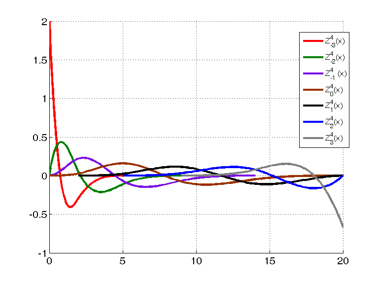
The basis functions of the space are plotted in Figure 7. Every spline can be written as
| (17) |
Thus, e.g., for the cubic spline with zero integral is plotted in Figure 6.

3 Smoothing spline in
In [12], the construction of smoothing splines in the space was studied, however using standard -spline basis functions . Now we are able to construct smoothing splines in this space with new basis functions . For this purpose, let data , , weights , , sequence of knots , , and a parameter be given. For arbitrary our task is to find a spline , which minimizes the functional
Note that the choice of parameter and , where stands for th derivation, affects smoothness of the resulting spline. Let us denote , , and . Regarding the representation (13) and matrix notation (16), the functional can be written as a quadratic function
| (18) |
see [10, 11, 12] for details. In fact the matrix
| (19) |
is positive definite, because , are basis functions. Upper triangular matrix has full row rank. is a diagonal matrix such that
with
and
Finally, stands for the collocation matrix, i.e.
Using the notation ,
| (20) |
and
it is possible to rewrite the quadratic function as
| (21) |
Our task is to find a spline which minimizes the functional , in other words, we want to find a minimum of the function (21). It is obvious that this function has just one minimum if and only if the matrix is positive definite (p.d.). From (20) it can be easily seen that
From Schoenberg-Whitney theorem and its generalization, see [2] and [10], it is known that matrix is of full column rank if and only if there exists with , , such that , . In this case from the necessary and sufficient condition for a unique minimum of quadratic function, i.e.
we get a system of linear equations and then the unique solution of this system is given by
| (22) |
Consequently, the resulting smoothing spline is obtained by the formula
in matrix notation using standard -splines as
where the vector is obtained as
.
4 Orthogonalization of basis functions
A further step is to orthogonalize the basis
of the space that is by construction obligue with respect to the space metric. For this purpose the idea presented in [19] is used. We search for a linear transformation such that
forms an orthogonal set of basis functions of the space , i.e.
Regarding the lemma presented in [19] and notation used here, we can formulate the following statement.
Lemma 4.1.
An invertible transformation orthogonalizes the basis functions if and only if it satisfies the condition that
where represents the positive definite matrix
With respect to the definition of basis functions the matrix can be expressed as
| (23) |
where . The linear transformation is not unique and can be computed for example by the Cholesky decomposition. The basis functions
are orthogonal and have a zero integral. The linear and quadratic -splines with zero integral and their orthogonalization are plotted in Figures 8 and 9.


To sum up, the spline with zero integral can be constructed as a linear combination of orthogonal splines having zero integral in a form
On the other hand, the standard and well-known -splines can be used to represent in matrix form
This formulation seems to be very useful because it allows us to use existing -spline codes in software R or Matlab, for example, the collocation matrix or computation of integrals in (19).
5 Compositional splines in the Bayes space
Construction of splines directly in has important practical consequences, however, it is crucial also from the theoretical perspective. Expressing splines as functions in enables to back-transform them to the original Bayes space using (5). It results in compositional -splines, obtained from (8) as
| (24) |
Accordingly, for instance -splines from Figures 1-5 can be now expressed directly in the Bayes space as -splines, see Figures 10-12. Note that -splines fulfill the unit integral constraint which is, however, not necessary for further considerations. As a consequence, it is immediate to define vector space of compositional polynomial splines of degree , defined on a finite interval with the sequence of knots . From isomorphism between and it holds that
Moreover, from isometric properties of clr transformation it follows that every compositional spline in can be uniquely represented as
| (25) |
-splines forming the basis are by the default setting (8) not orthogonal. Their orthogonalization can be done as described in Section 4, i.e. by employing with the back-transformation to .


The resulting compositional splines (with either orthogonal, or non-orthogonal -spline basis) can be used for representation of densities directly in . This is an important step in construction of methods of functional data analysis involving density functions, like for ANOVA modeling [22] or for the SFPCA method introduced in [9] and demonstrated in the next section. In the latter case -splines were indeed already used for construction of the procedure, although at the respective level of development the authors were not aware of that. With -splines one has a guarantee that methods are developed consistently in the Bayes space. Moreover, the possibility of having an orthogonal basis enables to gain additional features resulting from orthogonality of finite dimensional projection in combination with approximate properties of spline functions.
As usual, compositional splines can be tuned according to concrete problem, with the advantage of their direct formulation in the Bayes space sense.
Example 5.1.
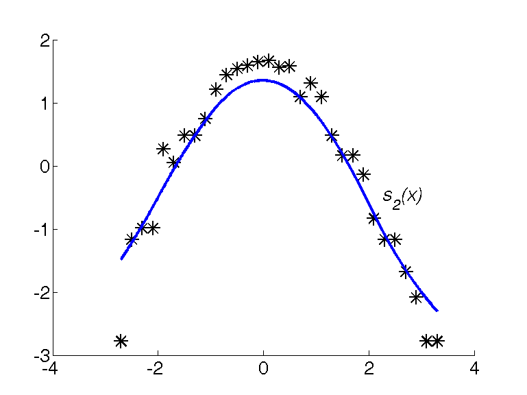
To illustrate smoothing of concrete data with a compositional spline, 1000 values from standard normal distribution were simulated and the support was determined by minimum and maximum simulated values, . Data were collected in a form of histogram, where the breakpoints are equidistantly spaced. The representative points of the histogram cells are denoted as asterisks in Figure 13 (left) and these points form the input data , for smoothing purpose. The -values stand for discretized relative contributions to the overall probability mass, therefore discrete clr transformation [1] is needed to obtain a real vector with zero sum constraint (Figure 13, right). These data points were smoothed using the procedure from Section 3 and back-transformed to the original space. In the concrete setting , , , , , were considered. The resulting spline with zero integral on interval is plotted in Figure 13 (right). In the left plot the compositional spline with unit integral by using (5) is depicted.

6 Application to anthropometric data
For the purpose of illustrating the smoothing procedure outlined in Section 3, a real-world data set dealing with the most commonly used anthropometric measure relating to body weight is presented. The data set we consider collects the body weight of apparently healthy Czech adolescents and young adults aged 15-31 years (the total of 4436 records) which were recruited non-randomly by offering free body composition assessment. Body weight was measured by the InBody 720 device (Biospace Co., Ltd, Seoul, Korea), recorded as the total body mass rounded to the nearest 0.1 kg.
The raw data for each of age groups, i.e. , , were turned into a form of histogram data as follows. The sampled values of the body weight in each age group were divided into equally-spaced classes of the united range 40-110 kg and the optimal number of classes, denoted by , , was set according to the well-known Sturge’s rule separately across the age groups. Because of the insufficient number of sampled data for males and females in each age group, gender information was ignored. Although there might be some differences between male and female samples due to sex dimorphism, they are not that dramatic (e.g., contrary to body height) because the weight is influenced also by external factors (nutrition, physical activity), and still allow for a reasonable aggregation of data. Subsequently, the proportions in classes within each age group were computed and present zero-values (zero counts in the respective classes) were imputed by values according to [13], where stands for the number of observations in th age group. Finally, the raw discretized density data which correspond to the midpoints of classes, (i.e., , were obtained by dividing (not necessary normalized) proportions of counts in classes by the length of the respective intervals resulting from partition of the weight range in each of age groups. Figure 14 shows four examples of histograms with different number of classes together with raw data (Table 1) to be smoothed. To do so, their transformation into real vectors is needed. We note that if the histogram data are constructed on subintervals of the same length, i.e. with equally-spaced breakpoints, it enables to use the discrete version of the clr transformation [1] directly on the vector of proportions by considering the scale invariance property. Otherwise, the input of the clr transformation must be vectors with raw density data in order to avoid misleading results which would not reflect the actual behavior of data. Vectors of clr transforms are hereafter denoted as for and clr values are listed in Table 2.
Having the collected data , we proceed to smooth them with the compositional smoothing splines using a system of -spline basis functions from the . They are considered on domain which has been modified in order to avoid undesired artifacts in densities at their right-hand side. For all observations, the same strategy was followed to set the values of the input parameters for the smoothing procedure. We employed cubic smoothing splines () with the given sequence of knots , the vectors of weights for all input data equal to vectors of ones and the smoothing parameter was set to . That is, when minimizing the penalized functional (18), the same importance is assigned to both smoothness of the smoothing splines as well as to their approximative properties. The resulting compositional smoothing splines are obtained via their clr representation
| (26) |
the corresponding -spline coefficients are reported in Table 3.
Figure 15(a) displays an example of three raw density data from Figure 14 together with smoothed curves in the space (right) and after the inverse transformation (5) in the space (left). The whole sample of smoothed density functions (Figure 15(b)) is plotted on blue scale distinguishing the age groups. Two trends are apparent – in the younger age groups, the estimated density functions are right skewed and exhibit lower variability while with increasing age they become more symmetric followed by higher variability. Nevertheless, density function in age group does not fully respect this behavior: the variability trend holds, but the distribution of weights is more similar to those in younger age groups as it is skewed more to the left. In general, it seems that adolescents appear to be predominantly of a lower body weight than the older persons whose weight is more spread over the weight classes and more pronounced in the middle part of the distribution. Accordingly, there is also a higher incidence of higher weights in comparison with the younger adolescents.
Importantly, the quality of smoothing is the same irrespective of the shape of the distribution. It might just happen that the smoothed densities exhibit heavier tails although they are not indicated by the data , even with some artifacts typical for overfitting. This is obviously due to keeping the zero integral constraint, which is more sensitive to deviations from monotonic character of densities at their tails. A possible way out, applied here, was to reduce slightly the range from to in order to keep predominantly the monotonic behavior of (normalized) counts at the right tails.
Of course, the smoothed data can be further analyzed using methods of functional data analysis [18], adapted in order to respect specific properties of densities. It is demonstrated here for case of the compositional functional principal component analysis (SFPCA) [9]. This statistical tool has been recently designed based on the Bayes space methodology, so it enables to capture the main modes of relative variability in a data set consisting of sampled density functions. Given a data set of zero-mean functional observations in , SFPCA aims to find the (normalized and orthogonal) directions of maximum variability in dataset, i.e., a collection of density functions called simplicial functional principal components (SPFCs) which maximize the following objective function over ,
| (27) |
where the orthogonality condition is assumed to be fulfilled for . Since represents a projection of along the direction , in fact we look for orthogonal basis functions in maximizing the relative variability of these projections. The maximization task (27) is efficiently implemented by applying the clr transformation (3) and the output can be back-transformed from the to the space, as detailed in [9].
The interpretation of SFPCs can be performed by displaying:
- •
individual SFPCs (as clr transformed density functions, SFPCs always represent contrasts between the parts of domain );
- •
overall mean density function along with its perturbation by SFPCs powered by a suitable constant,
(28) where is an amount of the variability of the dataset along the direction and it holds . This is a natural choice because SFPCs represent variation around the overall mean density function;
- •
the projection of dataset along the directions ,
where are so called principal component scores associated with the th SFPCs . The scores can be plotted for pairs of the first SFPCs to assess the relationship among sampled density functions or to reveal presence of outlying observations;
- •
to complete the above interpretation it is important to note that the original functions and the eigenfunctions are based on a -spline basis expansion
(29) respectively, by considering (26).
SFPCA is also a statistical method for reducing dimensionality of dataset. The number of SFPCs can be determined from the scree plot which displays cumulative percentage of the total variance explained by each subsequent SFPC. That is, the dimensionality is identified by a point in scree plot at which explained variability drops off.
For the actual computation, -splines (29) of the input functional observations, represented by the corresponding -splines (26), were expressed by -splines with -spline coefficients (listed in Table 4) using formula (16). The output of SFPCA for body weight density functions is reported in Figure 16. According to scree plot (Figure 16(b)), two or three SFPCs should be taken, but we resort to use only first two of them which capture together almost 85 of the total variability of the data set. The first SFPC (Figure 16(c)) represents the contrast between the weight below and above 78 kg, which could be considered as a reference (average) weight. Hence, higher scores along the SFPC1 are expected for age groups with higher incidence of individuals with higher body weight than the average, and, conversely, lower scores are associated with age groups with higher incidence of individuals with lower body weight then the average. The interpretation of SFPC1 can be obviously linked with age, see Figure 16(b). The scree plot more or less separates rather right skewed weight density functions of younger age groups (located on the left in the scree plot) from those more symmetric ones associated with older age groups (located on the right in the scree plot).
The second SFPC (Figure 16(d)) characterizes the variability within the tails of density functions, i.e. the main contribution to the variability along SFPC2 is provided by the lowest and highest weight values ( 51 kg and 98 kg respectively). It contrasts low and high weights (associated with high scores along the SFPC2) against middle weight values (associated with low scores along the SFPC2), see Figure 16(b). The consistent interpretation can be also observed from Figure 16(e) which displays the variation along the first two directions – SFPC1 and SFPC2 – with respect to sample mean (i.e. ).
Figures 16(f) and 16(g), respectively, represent two main modes of variability in the data set (). For instance, the variation along SFPC2 is confirmed to be exhibited in tails of density functions and the observations with lowest (gold curve) and highest score (red curve) further support the conclusions made so far. The high scores along the second direction thus reflect heavier tails and, conversely, the low scores along the second direction reflects low incidence of individuals with extreme (both small and high) weights. Nevertheless, the relationship of scores (Figure 16(b)) is apparent: at the beginning, they continue to fall, reach a bottom and then continue to grow. The relationship might be partially explained by unequal representation of men and women in age groups and unequal number of observations in these age groups. Another reason might be that data corresponding to age groups with low SFPC2 scores were collected mostly from students of the Faculty of Physical Culture at Palacký University in Olomouc, Czech Republic, which form more homogeneous population than an average one. In any case, the second SFPC reveals an interesting feature which is worth to be further investigated.
| 0.0656 | 0.2625 | 0.3375 | 0.2156 | 0.0750 | 0.0281 | 0.0094 | 0.0062 | |||||
|---|---|---|---|---|---|---|---|---|---|---|---|---|
| 0.0075 | 0.0300 | 0.0386 | 0.0246 | 0.0086 | 0.0032 | 0.0011 | 0.0007 | |||||
| 44.375 | 53.125 | 61.875 | 70.625 | 79.375 | 88.125 | 96.875 | 105.625 | |||||
| 0.0156 | 0.0869 | 0.1804 | 0.2138 | 0.2272 | 0.1514 | 0.0935 | 0.0200 | 0.0067 | 0.0045 | |||
| 0.0022 | 0.0124 | 0.0258 | 0.0305 | 0.0325 | 0.0216 | 0.0134 | 0.0029 | 0.0010 | 0.0006 | |||
| 43.5 | 50.5 | 57.5 | 64.5 | 71.5 | 78.5 | 85.5 | 92.5 | 99.5 | 106.5 | |||
| 0.0078 | 0.0908 | 0.2100 | 0.1971 | 0.1659 | 0.1659 | 0.1011 | 0.0259 | 0.0337 | 0.0017 | |||
| 0.0011 | 0.0130 | 0.0300 | 0.0282 | 0.0237 | 0.0237 | 0.0144 | 0.0037 | 0.0048 | 0.0002 | |||
| 43.5 | 50.5 | 57.5 | 64.5 | 71.5 | 78.5 | 85.5 | 92.5 | 99.5 | 106.5 | |||
| 0.0568 | 0.1023 | 0.2045 | 0.2386 | 0.2159 | 0.1364 | 0.0455 | ||||||
| 0.0057 | 0.0102 | 0.0205 | 0.0239 | 0.0216 | 0.0136 | 0.0045 | ||||||
| 45.0 | 55.0 | 65.0 | 75.0 | 85.0 | 95.0 | 105.0 |
| 0.100 | 1.486 | 1.737 | 1.289 | 0.233 | -0.748 | -1.846 | -2.252 | |||||
|---|---|---|---|---|---|---|---|---|---|---|---|---|
| 44.375 | 53.125 | 61.875 | 70.625 | 79.375 | 88.125 | 96.875 | 105.625 | |||||
| -0.210 | 1.217 | 1.760 | 1.636 | 0.396 | -0.392 | -2.001 | -2.407 | |||||
| 44.375 | 53.125 | 61.875 | 70.625 | 79.375 | 88.125 | 96.875 | 105.625 | |||||
| -1.375 | 0.570 | 1.316 | 1.669 | 1.381 | 0.534 | -0.364 | -2.069 | -1.663 | ||||
| 43.889 | 51.667 | 59.444 | 67.222 | 75.000 | 82.778 | 90.556 | 98.333 | 106.111 | ||||
| -1.354 | 0.592 | 1.419 | 1.443 | 1.406 | 1.131 | 0.563 | -0.661 | -1.171 | -3.369 | |||
| 43.5 | 50.5 | 57.5 | 64.5 | 71.5 | 78.5 | 85.5 | 92.5 | 99.5 | 106.5 | |||
| -1.536 | 0.628 | 1.408 | 1.555 | 1.535 | 1.209 | 0.302 | -0.774 | -1.536 | -2.789 | |||
| 43.5 | 50.5 | 57.5 | 64.5 | 71.5 | 78.5 | 85.5 | 92.5 | 99.5 | 106.5 | |||
| -1.341 | 0.674 | 1.333 | 1.558 | 1.638 | 1.452 | 0.422 | -0.568 | -2.034 | -3.133 | |||
| 43.5 | 50.5 | 57.5 | 64.5 | 71.5 | 78.5 | 85.5 | 92.5 | 99.5 | 106.5 | |||
| -1.746 | 0.451 | 1.185 | 1.463 | 1.411 | 1.131 | 0.531 | -0.242 | -1.746 | -2.439 | |||
| 43.5 | 50.5 | 57.5 | 64.5 | 71.5 | 78.5 | 85.5 | 92.5 | 99.5 | 106.5 | |||
| -1.168 | 0.550 | 1.281 | 1.450 | 1.511 | 1.106 | 0.624 | -0.917 | -2.015 | -2.421 | |||
| 43.5 | 50.5 | 57.5 | 64.5 | 71.5 | 78.5 | 85.5 | 92.5 | 99.5 | 106.5 | |||
| -1.884 | 0.573 | 1.412 | 1.348 | 1.177 | 1.177 | 0.681 | -0.680 | -0.417 | -3.388 | |||
| 43.5 | 50.5 | 57.5 | 64.5 | 71.5 | 78.5 | 85.5 | 92.5 | 99.5 | 106.5 | |||
| -1.602 | 0.595 | 1.186 | 1.274 | 1.106 | 0.796 | 0.056 | -0.423 | -2.988 | ||||
| 43.889 | 51.667 | 59.444 | 67.222 | 75.000 | 82.778 | 90.556 | 98.333 | 106.111 | ||||
| -1.401 | 0.471 | 0.768 | 0.824 | 1.145 | 0.850 | 0.209 | -1.178 | -1.688 | ||||
| 43.889 | 51.667 | 59.444 | 67.222 | 75.000 | 82.778 | 90.556 | 98.333 | 106.111 | ||||
| -1.045 | 0.513 | 0.901 | 1.180 | 1.258 | 0.513 | -0.485 | -2.836 | |||||
| 44.375 | 53.125 | 61.875 | 70.625 | 79.375 | 88.125 | 96.875 | 105.625 | |||||
| -0.816 | 0.570 | 0.742 | 0.742 | 1.056 | 0.570 | -0.256 | -2.608 | |||||
| 44.375 | 53.125 | 61.875 | 70.625 | 79.375 | 88.125 | 96.875 | 105.625 | |||||
| -1.155 | 0.579 | 0.790 | 0.965 | 0.690 | -0.308 | -1.561 | ||||||
| 45.0 | 55.0 | 65.0 | 75.0 | 85.0 | 95.0 | 105.0 | ||||||
| -1.060 | 0.480 | 0.837 | 0.674 | 0.614 | -0.773 | -0.773 | ||||||
| 45.0 | 55.0 | 65.0 | 75.0 | 85.0 | 95.0 | 105.0 | ||||||
| –0.756 | -0.168 | 0.525 | 0.679 | 0.579 | 0.120 | -0.979 | ||||||
| 45.0 | 55.0 | 65.0 | 75.0 | 85.0 | 95.0 | 105.0 |
| age group | spline coefficients, | ||||
|---|---|---|---|---|---|
| -6.950 | 6.647 | 46.536 | 40.973 | 13.163 | |
| -7.806 | -0.596 | 41.616 | 45.181 | 14.083 | |
| -16.677 | -11.292 | 18.284 | 43.917 | 9.102 | |
| -17.067 | -8.988 | 21.373 | 33.533 | 20.188 | |
| -18.483 | -9.902 | 22.408 | 38.249 | 16.447 | |
| -17.242 | -7.010 | 18.199 | 46.788 | 18.682 | |
| -20.452 | -10.875 | 11.653 | 36.887 | 14.797 | |
| -15.236 | -5.368 | 16.735 | 46.421 | 14.071 | |
| -22.485 | -12.348 | 17.033 | 23.450 | 20.153 | |
| -19.873 | -14.176 | 13.567 | 20.115 | 19.448 | |
| -19.011 | -5.949 | -4.623 | 30.860 | 9.973 | |
| -14.997 | -10.545 | 2.638 | 28.225 | 19.143 | |
| -14.461 | -4.455 | -0.689 | 21.892 | 18.070 | |
| -18.518 | -11.045 | -2.723 | 21.744 | 10.395 | |
| -16.445 | -9.417 | -1.814 | 23.562 | 2.889 | |
| -5.077 | -15.534 | -4.171 | 8.220 | 7.618 | |
| age group | spline coefficients, | |||||
|---|---|---|---|---|---|---|
| -1.264 | 1.236 | 2.381 | -0.332 | -2.472 | -2.289 | |
| -1.419 | 0.655 | 2.520 | 0.213 | -2.764 | -2.449 | |
| -3.032 | 0.490 | 1.766 | 1.530 | -3.095 | -1.583 | |
| -3.103 | 0.734 | 1.813 | 0.726 | -1.186 | -3.511 | |
| -3.361 | 0.780 | 1.929 | 0.946 | -1.938 | -2.860 | |
| -3.135 | 0.930 | 1.505 | 1.707 | -2.498 | -3.249 | |
| -3.719 | 0.871 | 1.345 | 1.507 | -1.964 | -2.573 | |
| -2.770 | 0.897 | 1.320 | 1.772 | -2.876 | -2.447 | |
| -4.088 | 0.922 | 1.754 | 0.383 | -0.293 | -3.505 | |
| -3.613 | 0.518 | 1.656 | 0.391 | -0.059 | -3.382 | |
| -3.456 | 1.187 | 0.079 | 2.118 | -1.857 | -1.734 | |
| -2.727 | 0.405 | 0.787 | 1.528 | -0.807 | -3.329 | |
| -2.629 | 0.910 | 0.225 | 1.348 | -0.340 | -3.143 | |
| -3.367 | 0.679 | 0.497 | 1.461 | -1.009 | -1.808 | |
| -2.990 | 0.639 | 0.454 | 1.515 | -1.838 | -0.502 | |
| -0.923 | -0.951 | 0.678 | 0.740 | -0.053 | -1.325 | |
7 Conclusions
The compositional splines, which enable to construct a spline basis in the clr space of density functions (-spline basis) and consequently also in the original space of densities (-spline basis), might become an important contribution within the Bayes space methodology for processing of functional data carrying relative information. They provide a solid theoretical base for further developments of the approximation theory in context of the Bayes spaces, but even more importantly, compositional splines can be used also for adaptation of popular methods of functional data analysis for density functions. Here the case of compositional functional principal component analysis was presented, but similarly, e.g., regression analysis or classification methods could be developed. Also further tuning of the compositional splines is possible, here represented by the smoothing compositional splines or by orthonormalization of the -basis. The latter case be used for an orthogonal projection of a density function on a subset of -splines, to further applications within the approximation theory or also for development of the theoretical framework of functional data analysis.
The pending challenge is to generalize the methodology introduced above also to dimensional density functions, , which can be formally extended from any univariate density to , where , in Equations (1) to (6); would be replaced by . Currently an approach which focuses on keeping the zero integral constraint of the clr transformed densities was developed in [8] as a generalization of [12], which, however, does not lead to a compositional counterpart of the -spline basis. A consistent approach in this direction is currently under development.
Acknowledgements
The authors gratefully acknowledge both the support by Czech Science Foundation GA18-09188S, the grant IGA_PrF_2018_024 Mathematical Models of the Internal Grant Agency of the Palacký University in Olomouc, and the grant COST Action CRoNoS IC1408.
References
- [1] J. Aitchison. The statistical analysis of compositional data. Journal of the Royal Statistical Society. Series B (Methodological), pages 139–177, 1982.
- [2] C. De Boor. A practical guide to splines, volume 27. Springer-Verlag New York, 1978.
- [3] P. Delicado. Dimensionality reduction when data are density functions. Computational Statistics & Data Analysis, 55(1):401–420, 2011.
- [4] P. Dierckx. Curve and surface fitting with splines. Oxford University Press, 1995.
- [5] M. L. Eaton. Multivariate statistics: a vector space approach. JOHN WILEY & SONS, INC., 605 THIRD AVE., NEW YORK, NY 10158, USA, 1983, 512, 1983.
- [6] J. J. Egozcue, J. L. Díaz-Barrero, and V. Pawlowsky-Glahn. Hilbert space of probability density functions based on aitchison geometry. Acta Mathematica Sinica, 22(4):1175–1182, 2006.
- [7] J. J. Egozcue, V. Pawlowsky-Glahn, G. Mateu-Figueras, and C. Barcelo-Vidal. Isometric logratio transformations for compositional data analysis. Mathematical Geology, 35(3):279–300, 2003.
- [8] D. Guégan and M. Iacopini. Nonparametric forecasting of multivariate probability density functions. arXiv preprint arXiv:1803.06823, 2018.
- [9] K. Hron, A. Menafoglio, M. Templ, K. Hruzová, and P. Filzmoser. Simplicial principal component analysis for density functions in bayes spaces. Computational Statistics & Data Analysis, 94:330–350, 2016.
- [10] J. Machalová. Optimal interpolating and optimal smoothing spline. Journal of Electrical Engineering, 53:79–82, 2002.
- [11] J. Machalová. Optimal interpolatory splines using -spline representation. Acta Universitatis Palackianae Olomucensis. Facultas Rerum Naturalium. Mathematica, 41(1):105–118, 2002.
- [12] J. Machalova, K. Hron, and G. S. Monti. Preprocessing of centred logratio transformed density functions using smoothing splines. Journal of Applied Statistics, 43(8):1419–1435, 2016.
- [13] J.-A. Martín-Fernández, K. Hron, M. Templ, P. Filzmoser, and J. Palarea-Albaladejo. Bayesian-multiplicative treatment of count zeros in compositional data sets. Statistical Modelling, 15(2):134–158, 2015.
- [14] A. Menafoglio, A. Guadagnini, and P. Secchi. A kriging approach based on aitchison geometry for the characterization of particle-size curves in heterogeneous aquifers. Stochastic Environmental Research and Risk Assessment, 28(7):1835–1851, 2014.
- [15] A. Menafoglio, A. Guadagnini, and P. Secchi. Stochastic simulation of soil particle-size curves in heterogeneous aquifer systems through a bayes space approach. Water Resources Research, 52(8):5708–5726, 2016.
- [16] V. Pawlowsky-Glahn and J. J. Egozcue. Geometric approach to statistical analysis on the simplex. Stochastic Environmental Research and Risk Assessment, 15(5):384–398, 2001.
- [17] V. Pawlowsky-Glahn, J. J. Egozcue, and R. Tolosana-Delgado. Modeling and analysis of compositional data. John Wiley & Sons, 2015.
- [18] J. Ramsay. Functional data analysis. Encyclopedia of Statistics in Behavioral Science, 2005.
- [19] A. Redd. A comment on the orthogonalization of b-spline basis functions and their derivatives. Statistics and Computing, 22(1):251–257, 2012.
- [20] R. Talská, A. Menafoglio, J. Machalová, K. Hron, and E. Fišerová. Compositional regression with functional response. Computational Statistics & Data Analysis, 123:66–85, 2018.
- [21] K. G. Van den Boogaart, J. J. Egozcue, and V. Pawlowsky-Glahn. Bayes linear spaces. SORT: statistics and operations research transactions, 2010, vol. 34, núm. 4, p. 201-222, 2010.
- [22] K. G. Van den Boogaart, J. J. Egozcue, and V. Pawlowsky-Glahn. Bayes hilbert spaces. Australian & New Zealand Journal of Statistics, 56(2):171–194, 2014.