Planetary Nebulae and How to Find Them: Color Identification in Big Broadband Surveys
Abstract
Planetary nebulae (PNe) provide tests of stellar evolution, can serve as tracers of chemical evolution in the Milky Way and other galaxies, and are also used as a calibrator of the cosmological distance ladder. Current and upcoming large scale photometric surveys have the potential to complete the census of PNe in our galaxy and beyond, but it is a challenge to disambiguate partially or fully unresolved PNe from the myriad other sources observed in these surveys. Here we carry out synthetic observations of nebular models to determine color-color spaces that can successfully identify PNe among billions of other sources. As a primary result we present a grid of synthetic absolute magnitudes for PNe at various stages of their evolution, and we make comparisons with real PNe colors from the Sloan Digital Sky Survey. We find that the versus , and the versus , color-color diagrams show the greatest promise for cleanly separating PNe from stars, background galaxies, and quasars. Finally, we consider the potential harvest of PNe from upcoming large surveys. For example, for typical progenitor host star masses of 3 M⊙, we find that the Large Synoptic Survey Telescope (LSST) should be sensitive to virtually all PNe in the Magellanic Clouds with extinction up to of 5 mag; out to the distance of Andromeda, LSST would be sensitive to the youngest PNe (age less than 6800 yr) and with up to 1 mag.
Subject headings
planetary nebulae: general—stars: evolution—surveys—techniques: photometricI. Introduction
Planetary Nebulae (PNe) are the shells of gas ionized by hot central stars. The PN forms from previously ejected material lost during the asymptotic giant branch (AGB) phase of a low-to-intermediate mass star (). The central star of a planetary nebula (CSPN) plays a key role in the PN characteristics since its fast stellar wind plows into the AGB wind to form the nebula while the CSPN’s high surface temperature photoionizes the gas in the newly-formed nebula. A PN will expand and fade over time, while the CSPN rises in temperature, until it eventually cools towards the white dwarf (WD) cooling track (Kwok et al. 1978; Vassiliadis & Wood 1994; Bloecker 1995; Miller Bertolami 2016). Compared to the lifetime of the star, the PN phase is short-lived remaining visible for only years (Iben 1995; Jacob et al. 2013).
For over 60 years the formation process of PNe has been questioned favoring two contending processes. The first consists of a single star in which heavy mass loss occurs during the AGB phase while stellar rotation and magnetic fields shape the expanding nebula (Gurzadian 1962; Garcia-Segura et al. 1999; Garcia‐Segura et al. 2005; Matt et al. 2004; Blackman 2004). The second process favors a wide range of interactions between the evolving star and a binary companion for shaping the nebula (Fabian & Hansen 1979; Soker 1997; De Marco 2009). Theoretical and observational considerations suggest that a single AGB star is unlikely to produce a strong enough magnetic field to dramatically shape the nebula, favouring the possibility of binary interactions being mainly responsible for the formation and shaping of non-spherical PN (Soker 2006; Nordhaus et al. 2007). It is likely that there are still many PNe left undiscovered as our best estimates place the total number of galactic PNe anywhere between and depending on the formation process (De Marco 2005; Moe & De Marco 2006).
Naturally, because they represent a specific and short-lived phase of stellar evolution, PNe can be difficult to study but they are important for improving our understanding of late-stage low- to intermediate-mass stars (Iben 1995; Frew 2008). PNe that have been found in the Milky Way and in neighboring galaxies have been extremely valuable for a variety of studies. Because of their bright emission lines, PNe are identifiable across the Galaxy and in nearby stellar systems. PNe can be used as tracers of galaxy kinematics (Hurley-Keller & Morrison 2004; Peng et al. 2004; Merrett et al. 2006; Coccato & Coccato 2016); as a rung on the distance ladder via the PN luminosity function (Ciardullo 2003; Gesicki et al. 2018); and as potential tracers of the chemical evolution of the Milky Way and other galaxies (Walsh et al. 1997; Richer et al. 1998; Kniazev et al. 2008; Saviane et al. 2009; Magrini & Gonçalves 2009; Kwitter et al. 2012; Sanders et al. 2012; Cavichia et al. 2017).
There is ongoing interest in techniques for readily identifying more PNe efficiently and reliably. A large number of PNe have been discovered through techniques that take advantage of their bright nebular emission lines. surveys such as the SuperCOSMOS Survey (SHS) (Parker et al. 2005; Frew et al. 2014), the INT Photometric Survey (IPHAS) (Drew et al. 2005), and the VST Photometric Survey (VPHAS+) (Drew et al. 2014) have been very successful in identifying galactic PNe and are cataloged in the Hong Kong/AAO/Strasbourg/ (HASH) (Parker et al. 2016) database which contains objects. Integral field spectroscopy of [O III] has been used to find PNe in crowded areas (Pastorello et al. 2013). Dust can make it difficult for optical surveys to detect PNe but they have also been found in the UKIRT Wide-field Imaging Survey for survey (UWISH2) through their emission (Gledhill et al. 2018). More galactic PNe have recently been discovered through their multi-wavelength characteristics ranging from optical to radio emission (Fragkou et al. 2018).
Large, all-sky surveys, like the Sloan Digital Sky Survey (SDSS) and, in the future, the Large Synoptic Survey Telescope (LSST), can be used to potentially identify thousands of new PN based on broadband photometry where PNe are poorly characterized. Although the observed broadband colors of PNe have been studied (Schmeja & Kimeswenger 2001; Frew & Parker 2010; Iłkiewicz & Mikołajewska 2017, e.g., in 2MASS and WISE colors), and although the theoretically expected broadband colors of PN central stars have previously been calculated (Weston et al. 2009; Morris & Montez 2015, e.g.,), the theoretically expected broadband colors of PN nebular emission have yet to be characterized and compared with observations. Existing PNe catalogs are far from complete, and upcoming all-sky photometric surveys have great potential to uncover troves of additional PNe, assuming that it will be possible to efficiently distinguish true PNe from the large numbers of false positives.
We focus on the optical region of the PN spectrum because of the prominent nebular emission lines at these wavelengths. A vast amount of survey data is or will become available through SDSS and LSST, therefore we attempt to characterize PNe in this photometric system. We consider the broadband characteristics of a synthetic PN as a function of evolutionary age, for both resolved and unresolved PNe. Our methodology for creating our synthetic PN models and calculating the synthesized observations are presented in §II. A grid of broadband absolute magnitudes and the efficacy of different color-color diagrams to reliably identify PNe are provided in §III. In §IV we compare our results to existing observational SDSS studies and consider future applications with LSST. Finally, §V presents a summary of our conclusions.
II. Methodology
In this section, we describe our methodology for creating synthetic broadband observations of PNe as functions of evolutionary age for both resolved and unresolved PNe. We begin by describing the physical ingredients and assumptions adopted. Because we seek to undertake a more comprehensive study of the broadband behavior of PNe than previously attempted, we intentionally construct our methodology to fully and self-consistently include the effects of both the central star and the nebular evolution. Next we describe the production of the nebular spectra followed by the synthetic magnitudes and colors from these spectra, and we discuss our treatment of resolved and unresolved PNe. Finally, we include the effects of interstellar reddening for resolved and unresolved spectra.
II.1. Planetary Nebula Ingredients
To build our synthetic PN we start with the central star and nebular properties. In particular, throughout this study we work with a 3 progenitor star, because it is for such a star that nebular evolution models exist to which we can self-consistently couple the evolution of the central star and thereby produce synthetic spectra and colors over the course of the evolution of the star+PN. Figure 1 depicts the HR diagram for a central star evolutionary track from the models of Vassiliadis & Wood 1994; Bloecker 1995, along with and progenitor masses for context. The final mass of the white dwarf in this model is , similar to the 0.6 M⊙ mass that is often assumed as a fiducial mass for PN central stars (Perinotto et al. 2004). Thirteen specific age positions on the evolutionary track are indicated, representing the discrete ages that we have chosen to include in our study, spanning the evolution of the system from emergence of the PN to exposing the white dwarf. Figure 2 (top panel) indicates the temporal behavior of the CSPN luminosity () and temperature () corresponding to these 13 ages.


For every age position on the central star’s evolutionary track (Figure 1) we require a nebular emission model corresponding to that evolutionary age and with the appropriate central star mass. Fortunately, 1D radiation-hydrodynamics simulations of a PN have been performed by Perinotto et al. 2004; Schönberner et al. 2005. Because those simulations were done for the expansion of a PN illuminated by a central remnant of 0.595 , it is essential to use a central-star evolutionary model that produces a remnant as close to this same final mass as possible. That is why our choice above is of a central star whose final mass is most similar to this value11 1 The slight discrepancy between the central star final masses of 0.595 versus 0.605 in the nebular versus central star evolutionary tracks, respectively, is negligible for compact nebula with radii (Jacob et al. 2013)., corresponding to a progenitor mass of 3 .
We calculate the nebular size at each time step using a simple approximation based on the Perinotto et al. 2004; Schönberner et al. 2005 nebular model. Based on the radiation-hydrodynamic simulations, the densest part of the nebula is coincident with the inner radius (or rim), , which follows the relationship , where pc, yrs, , and . For each time step in the evolutionary track, we determine the inner radius () based on this prescription. Since the prescription is only applicable for yrs, we only considered the evolutionary track between these ages. As a result, the radii of our synthetic nebula model expands from pc to pc.
The outer radius of the nebula is determined by Cloudy calculations (see next section), specifically by a mass stopping criteria for each model. Phillips 2007 describe an empirical relationship to the total ionized mass, . increases linearly for according to until reaching a constant total mass, , for . In our radiative transfer calculations, we restrict the total ionized mass of the nebula according to this empirical relationship using . As a result the final mass of our synthetic nebula are designed to closely match the final masses of the ionized nebula described in Phillips 2007. Also as a consequence of this stopping mass criteria the thickness of the nebular shell remains thin, specifically, is always 0.25.
In addition to the inner radius, for each considered position on the evolutionary track we must calculate the electron density, , of the nebula. Based on the behavior of Galactic and Magellanic PNe Frew 2008 derived a nebular density relation with nebular radius of , where is the electron density of the nebula and is the nebular radius, in our case . Figure 2 (bottom panel) shows the evolution of and over all ages of the nebula.
II.2. Cloudy, With a Chance of Photons
The central star and nebular properties described in the previous section are used as input to Cloudy radiative transfer calculations. Cloudy is a plasma simulation software that simulates non-equilibrium gas conditions to predict an observable spectrum(version 13.03; Ferland et al. 2013).
In Table 1, we list the stellar and nebular ingredients needed to run our Cloudy radiative transfer models. For the nebular composition we use chemical abundances typical of a planetary nebula (Ferland et al. 2013; Aller & Czyzak 1983; Khromov 1989, see Table 2). We assume spherical geometry for the nebula, a uniform filling factor of unity, and no stopping temperature criteria. Distance between the observer and the nebula is assumed to be 1 kpc. The resulting coarse (R = 200) and high-resolution (R = 2000) spectra at the youngest nebular age considered ( yrs, K, ) are shown in Figure 3 for our region of interest (). The high-resolution spectrum is used for display purposes. Since the high-resolution spectrum does not preserve flux, we use the coarse spectrum for our photometric calculations.
| (yrs) | (K) | () | (pc) | () | () |
|---|---|---|---|---|---|
| 3502 | 4.786 | 3.782 | 0.035 | 4.386 | 0.071 |
| 4154 | 4.887 | 3.766 | 0.044 | 4.159 | 0.088 |
| 4860 | 4.988 | 3.736 | 0.056 | 3.911 | 0.113 |
| 5663 | 5.089 | 3.671 | 0.073 | 3.652 | 0.146 |
| 6328 | 5.155 | 3.571 | 0.088 | 3.460 | 0.178 |
| 6745 | 5.183 | 3.468 | 0.098 | 3.349 | 0.199 |
| 7031 | 5.194 | 3.363 | 0.106 | 3.277 | 0.201 |
| 7224 | 5.195 | 3.257 | 0.111 | 3.230 | 0.201 |
| 7387 | 5.181 | 3.056 | 0.115 | 3.192 | 0.202 |
| 7453 | 5.165 | 2.912 | 0.117 | 3.176 | 0.202 |
| 7552 | 5.140 | 2.73 | 0.119 | 3.153 | 0.203 |
| 7751 | 5.114 | 2.566 | 0.125 | 3.108 | 0.202 |
| 8351 | 5.095 | 2.452 | 0.142 | 2.980 | 0.202 |
| Atom | [X/H] |
| (dex) | |
| H | 0.0000 |
| He | -1.0000 |
| C | -3.1079 |
| N | -3.7447 |
| O | -3.3565 |
| F | -6.5229 |
| Ne | -3.9586 |
| Na | -5.7212 |
| Mg | -5.7959 |
| Al | -6.5686 |
| Si | -5.0000 |
| P | -6.6990 |
| S | -5.0000 |
| Cl | -6.7696 |
| Ar | -5.5686 |
| K | -6.9208 |
| Ca | -7.9208 |
| Fe | -6.3010 |
| Ni | -7.7447 |

II.3. Synthesizing Broadband Photometric Observations
We consider observations of our synthetic nebulae performed with a standard photometric system22 2 We used the LSST filters as defined on 2016-12-07 obtained from the Spanish Virtual Observatory (SVO) Filter Profile Service. The filter is shown for completeness but is not used in this study.. The set of photometric filters cover wavelengths between 320 nm and 1080 nm and their properties are provided in Table 3 with their transmission curves shown in Figure 3. The filter transmission curve is interpolated onto the wavelength grid of the coarse resolution Cloudy spectra described in §II.2. For each age of our synthetic nebula we convolved the nebular and central star flux spectra with the filter transmission curves. Then we normalized the resulting flux to the AB magnitude system to determine the magnitudes. We scaled these magnitudes to 10 pc to determine the absolute magnitudes, which are presented in Table 4.
| Filter | Range | ||||
|---|---|---|---|---|---|
| (nm) | (nm) | (nm) | (mags) | (mags) | |
| 320–400 | 373.2 | 54.6 | 14.7 | 23.9 | |
| 400–552 | 473.0 | 133.2 | 15.7 | 25.0 | |
| 552–691 | 613.8 | 133.7 | 15.8 | 24.7 | |
| 691–818 | 748.7 | 832.5 | 15.8 | 24.0 | |
| 818–922 | 866.8 | 937.5 | 15.3 | 23.3 | |
| aafootnotemark: | 950–1080 | 967.6 | 81.0 | 13.9 | 22.1 |
II.4. Accounting for Spatially Resolved Extended Emission
The extended nature of a PN requires additional consideration. For aperature photometry, when the nebula and central star are resolved only a fraction of the nebular flux will be measured. To understand the impact of resolved nebula and central stars, we constructed a toy model of the synthetic nebulae. For each stage, we assumed a three-dimensional spherical shell with the radius, thickness, and density used in our synthetic nebulae. We projected this shell onto the plane of the sky. Assuming aperture photometry, we considered a range of aperture diameters on the sky, , and nebular diameter on the sky, . For a range of aperture to nebular diameter ratios, , we calculated the fraction of nebular emission, , that is measured by the aperture. We recalculated the magnitudes after scaling the nebular flux by this fraction and adding it to the central star flux. We consider models with the same nebular fraction as a fractional variant and label them with roman numerals in increasing order as decreases.
This method of estimating resolved nebular magnitudes provides the most flexibility with regards to survey resolution characteristics. Note that because in reality a given PN, at a given distance, will evolve in its apparent angular size, it will not in general evolve along a single variant “track”. Rather, the collection of variant tracks represent the overall parameter space through which individual PNe may evolve, for a range of distances, photometric apertures, and states of evolution.
II.5. Reddening
Intervening dust poses a serious problem for observing and identifying objects with photometric colors. The dust will dim (extinction) and redden an object which can limit the distance at which an object can be detected and change its position in a color-color diagram. To determine the reddening vector in the ugrizy system, we applied the reddening curve of Cardelli et al. 1989 to all ages of the synthetic nebular spectra then calculated the reddened magnitudes. Figure 4 shows how varying levels of extinction () can affect the spectrum of a PN. Figures 5 and 6 show the reddening vector that all 13 models would follow with .

III. Results
In this section, we present the main results of our study. First, we provide a grid of synthetic photometry representing our model PN at different evolutionary ages and different observed angular sizes. Second, we describe the evolution of prominent emission lines in each filter and their effect on the calculated magnitudes. We then identify the color-color spaces that are most effective at differentiating PNe from other celestial objects.
III.1. Synthesized Nebula Absolute Magnitudes
A key result of this study is the collection of the absolute magnitudes for our synthetic nebulae in the photometric system (see Table 4, Table 5 and Figure 5 for all variants). These absolute magnitudes span years of PN evolution for a progenitor star evolving into a white dwarf. The contributions from continuum and line emission dictate the behavior of the broad band magnitudes as a function of age. In each band, the continuum drops by about an order of magnitude as the models approach older stages resulting in the overall decline in the broadband magnitudes as the nebula evolves. We do not display variants beyond VII, as variants VIII–X become too faint to be practical.
The line emission as a function of age in each band is often dictated by one or two species that dominate a given bandpass. In the band, the prominent emission lines are: [Ne III] (, ), [O II] (, ), H II (, , ), and He III (). In the band, the prominent emission lines are: [O III] (, ), H I ( , , ), He II (), He I (), [S II] (, , ), and N I (, ). In the band, the prominent emission lines are: H I ( ), [N II] (, ), He I (), [S II] (, , ), S III (), [Cl III] () and [O I] (). In the band, the prominent emission lines are: [Ar III] (, ), [O II] (, ), He I (), and Cl IV (). Fluxes from the aforementioned lines exhibit three common behaviors: (1) decreasing throughout the evolution, (2) double-peaked with an initial rise, a decrease, then another rise as the CSPN approaches its hottest temperature before decreasing again as cools, and, (3) single-peak with a steady increase in flux as the as CSPN approaches its hottest temperature before decreasing as cools. Lines with decreasing behavior are: [Ne III], H I, [O III], He I, S III, [Cl III], Cl IV, [Ar III]. Lines with a double peak behavior are: [O II], [S II], N I, [N II], [O I]. Only He II lines show a single peak behavior. These behaviors of the line emission are due to the ionization and physical parameters (radius and density) of the modeled nebula.
When convolved with the bandpass transmission curves the broadband magnitudes can mimic the age-related behavior of the strongest emission lines. The band magnitude behavior is double-peaked with a steady decrease largely influenced by the [O II] emission and the overall decreasing flux from the other lines in this bandpass. The [Ne III] lines are very close to the edge of the filter bandpass, where the transmission is reduced, therefore, despite being the most prominent line in the band, [Ne III] does not contribute as much flux as the [O II] lines. The band magnitude exhibits decreasing behavior and is largely influenced by [O III]. The band magnitude is double-peaked, which is the result of the H I emission dominating at earlier ages () until [N II] begins to dominate. The band magnitude decreases according to the evolution of [Ar III] with some influence from [O II].
In the CMDs (Figure 5) there exists a hook feature before the eighth model ( yrs) (also somewhat visible in the CCDs) due to the evolution of these lines. Once the models have reached the empirically observed maximum mass we imposed (at the eighth model yrs) they become matter bounded and transparent to ionizing radiation resulting in a somewhat steady decline in brightness and color evolution.


The absolute magnitudes given in Table 4 are only valid for the total integrated flux from a PN. When a PN is resolved, only a fraction of the nebula will be observed, thus reducing the nebular contribution. This effect changes the measured flux in each filter and the measured color for any two filters. Figures 5, 6, and 8 show how magnitudes and colors change as the aperture encloses less of the nebula.
| Variant I: | = | |||||
|---|---|---|---|---|---|---|
| Age | ||||||
| (yrs) | (mags) | (mags) | (mags) | (mags) | (mags) | (mags) |
| 3502 | -2.59 | -3.63 | -3.38 | -2.20 | -2.18 | -2.09 |
| 4154 | -2.70 | -3.91 | -3.47 | -2.21 | -2.20 | -2.15 |
| 4860 | -2.46 | -3.94 | -2.98 | -1.87 | -1.98 | -1.94 |
| 5663 | -2.11 | -3.66 | -2.53 | -1.44 | -1.62 | -1.66 |
| 6328 | -1.93 | -3.41 | -2.36 | -1.21 | -1.40 | -1.49 |
| 6745 | -1.95 | -3.23 | -2.43 | -1.14 | -1.29 | -1.39 |
| 7031 | -1.98 | -3.00 | -2.53 | -1.06 | -1.13 | -1.28 |
| 7224 | -2.00 | -2.72 | -2.64 | -0.98 | -0.98 | -1.21 |
| 7387 | -1.71 | -2.10 | -2.49 | -0.63 | -0.54 | -0.95 |
| 7453 | -1.44 | -1.60 | -2.27 | -0.33 | -0.18 | -0.72 |
| 7552 | -1.09 | -0.90 | -1.98 | 0.08 | 0.28 | -0.45 |
| 7751 | -0.75 | -0.22 | -1.68 | 0.45 | 0.71 | -0.24 |
| 8351 | -0.51 | 0.24 | -1.46 | 0.73 | 1.00 | -0.11 |
III.2. Identifying PNe in Color-Color Diagrams
We compare our PN models and variants to SDSS objects in Figure 6. Contours of stars, galaxies, and quasars are used to illustrate their locations in the various diagrams. Data for these object types come from SDSS DR7 (Abazajian et al. 2009) and were queried using the SDSS SkyServer. We only included objects with SDSS spectroscopic observations to allow for further filtering on for the star, galaxy, and quasar object types.
The top panel of Figure 6 shows the vs color-color diagram. Here, models occupy a separated space from the SDSS data with between 0 and and between 1.75 and . The unresolved synthetic nebular models (variant I), as well as the oldest resolved models (variants VI through IX) remain separated from stars, quasars, and galaxies through out all or most stages of evolution in this diagram for . (We do not show variants II–V as these are effectively equivalent to variant I.) As the central star and nebula are resolved, the colors converge towards the locus of blue evolved stars, as expected. Similarly, the bottom panel of Figure 6 shows that our models are also separated from most of the SDSS data in the vs color-color diagram for . These two diagrams will be essential in identifying new PN candidates of all ages.
In the middle panel of Figure 6, the PN models occupy the left region of the diagram. They fall between values of 1.75 to in and 1.6 to in . Our synthetic nebulae cross through the loci of early-type MS stars, quasars, and blue evolved stars in this diagram. The youngest ( yrs) and oldest ( yrs) stages in our fully unresolved models (variant I) are somewhat separated from these loci making these areas good places to look for young and old unresolved PN candidates. The change in color values for all CCDs is a result of the nebular emission as seen in Figure 5 and is described in the previous section.


IV. Discussion
IV.1. Comparison to Prior Work
A number of studies have shown that emission line objects like PNe can be identified or characterized by broadband filters. In the UV, optical, and near-infrared (NIR) Veyette et al. 2014 used Hubble Space Telescope (HST) Advanced Camera for Surveys and the Panchromatic Hubble Andromeda Treasury (PHAT) survey data to identify broadband detections of known PNe and were able to roughly estimate the excitation classifications of groups of PNe with the addition of archival m5007 narrow-band magnitudes. In the optical, Kniazev et al. 2014 used the Sloan Digital Sky Survey (SDSS) colors to separate PNe from other point sources in the outskirts of M31. Parker et al. 2016 developed a method using mid-infrared colors to identify galactic PN candidates using available data in the Galactic Legacy Infrared Mid-Plane Survey Extraordinaire I (GLIMPSE I) point source archive. Data from the Infrared Astronomical Satellite (IRAS) was used to inform optical spectroscopic follow-up by Suárez et al. 2006 to confirm PNe candidates along with post-AGB stars and sources transitioning from AGB to PN stages of evolution. Corradi et al. 2008 and following papers in the series (Corradi et al. 2010; Rodríguez-Flores et al. 2014) describe a similar method for selecting symbiotic star candidates using the INT Photometric Survey (IPHAS) and the Two Micron All Sky Survey (2MASS) colors showing that symbiotic stars can be distinguished from PNe through colors but ultimately spectroscopic follow-up is necessary for verification.
We compare our predicted PNe colors and magnitudes (for variant I) to confirmed PNe in M31 (Kniazev et al. 2014). Kniazev et al. 2014 used 29 known PNe in M31 (Jacoby & Ford 1986; Nolthenius & Ford 1987) to construct magnitude and color criteria to identify additional PNe with SDSS photometry. 70 were confirmed to be PNe through follow-up spectroscopy (Kniazev et al. 2014). In Figure 7 the color-magnitude and color-color diagrams presented in Kniazev et al. 2014 are reproduced along with some of their selection criteria. We queried SDSS (Abolfathi et al. 2018, DR14;) for clean sources within 1 degree of M31 and with point source criteria outlined in Kniazev et al. 2014. The spectroscopically verified PNe from Nolthenius & Ford 1987 along with our 3 PN evolutionary models scaled to the distance of M31 (van den Bergh 1999, 760 kpc;) are overlaid onto the CMD and CCD. At such a distance, all of our nebular models are unresolved. In the CMD, the sample identified by Kniazev et al. 2014 is consistent with the youngest stages of our PN models ( years). We find similar consistency in the CCD, except for youngest stage ( years), which is outside of the color cut used by Kniazev et al. 2014 to reduce contamination from high redshift objects. As suggested by our PN models, this color cut will limit the identification of the youngest and oldest PNe in M31, however, these PNe might be present and identifiable using the CCD.
We also compared our results for resolved and unresolved colors and magnitudes to six faint PNe (PN G094.0+27.4, PN G211.4+18.4, PN G049.3+88.1, PN G025.3+40.8, PN G047.0+42.4, and PN G158.8+37.1) recovered by Yuan & Liu 2013 through identification of excess or emission in the SDSS spectra of objects who’s photometry was affected by the nebula. For each PN, we used the object’s coordinates to obtain an SDSS g band image of the region (Abolfathi et al. 2018, DR14;) and visually identified the PN in the image (using ds9). We then visually located the closest object to the CS position of the PN and obtained the SDSS ugriz magnitudes of that source. In Figure 8 we compare the colors of these six sources in relation to our models. The colors for PN G094.0+27.4, PN G211.4+18.4, PN G047.0+42.4, and PN G158.8+37.1 are consistent with that expected from a central star with very little nebular emission as they appear close to our model variants VIII-X (marked as stars in Figure 8). The nebular radii of these three objects are > , which is much larger than the typical seeing resolution limit of SDSS, hence only a small fraction of the nebular emission is detected in these objects. PN G025.3+40.8 (marked as a triangle in Figure 8), with a nebular radius of , is consistent with a higher fraction of nebular flux detected as it appears near our variant VI models indicating a fractional nebular flux of was observed with the CS. PN G049.3+88.1 (marked as a circle in Figure 8), with a nebular radius of , is consistent with nearly all of the nebular flux detected as it appears near our variant I models. While this is not a rigorous comparison of these sources to our models, generally, we see that CSPNe with a larger sized nebula contain less nebular flux than CSPNe with a smaller sized nebula as predicted by our models.


IV.2. Applications to Upcoming Surveys
Upcoming surveys such as LSST can potentially greatly expand the number of known PNe at different stages of evolution, both within the Milky Way and in other nearby galaxies. As an example, other authors have estimated LSST’s distance limit for RR Lyrae variables to be 400 kpc (LSST Science Collaboration et al. 2009); LSST’s potential reach for PNe may also be similarly impressive. LSST will commence operations in 2023 and is scheduled to be a 10-year long survey of the southern sky aiming at addressing questions from scales of the solar system to dark energy. The telescope harbors an 8.4 meter mirror and a 3,200 megapixel camera that will image 37 billion stars and galaxies. The camera is equipped with the filter set with sensitivity information detailed in Table 3.
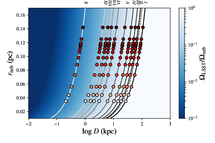
The first consideration for LSST’s reach of PNe is spatial resolution of PNe flux. The optimal seeing limit for LSST is projected to be (LSST Science Collaboration et al. 2009), if we take this as an estimate of the size of aperture (), then for any the nebula will potentially be resolved. In Figure 9, we calculate the ratio for a range of distances and include the locations of our synthetic nebular models shown in Figures 5 and 6. At a distance to the Magellanic Clouds (Pietrzyński et al. 2013; Graczyk et al. 2014, 49.97 and 62.1 kpc;) young models () are unresolved while older models are marginally resolved. For our oldest models () the nebular diameters are . With worse seeing or by utilizing a slightly adjustable aperture in the imaging analysis, it is possible to observe all the nebular flux for marginally-resolved cases.
The reach for a given survey is also dependent on the survey saturation and limiting magnitudes (LSST Science Collaboration et al. 2009, see Table 3;), as well as extinction to the source. Using Table 4, it is possible to study unresolved nebular fluxes for specific combinations of distance and extinction to determine the reach for LSST. Because the identification of potential PNe requires detection in at least three filters (, , and ) we considered the saturation and 5 limiting magnitudes, and , respectively, for these three filters. In Figure 10, we determined the LSST detection limit for our unresolved nebular models as a function of distance and extinction. For modest extinction values () at the LMC/SMC, all of our nebular models predict detectable emission in , , and , however, we potentially reach the saturation limit in and , for our youngest models when extinction drops below 1 mag (see Figure 10). For another example, if LSST observed a system like Andromeda (M31) at a distance of 760 kpc (van den Bergh 1999), in the areas of low extinction (), similar to those found in the outskirts of that galaxy (Kniazev et al. 2014; Dalcanton et al. 2015), the youngest nebular models can be detected in these three bands, but fewer of the older nebular models would be detected in (). Hence, surveys like LSST can be used to discover many new potential PNe beyond our galaxy.
We can also consider LSST’s reach for PNe specifically within the Milky Way. Here, estimating the reach is further complicated by the numerous combinations of nebular age/size, distance, and extinction. The contribution of the nebular flux to the aperture is a strong function of (see Figure 5). To consider the reach within the Milky Way, we provide variants of the absolute magnitudes in Table 5 for a range of . For example, we considered the distance- based reach for LSST at a distance consistent with the galactic center (Majaess et al. 2018, 8.3 kpc;). Young PNe (, ) will be resolved at the galactic center with only 1.6% of the nebular emission measured by a aperture (). As a result, such a PN would be detectable in , , and for lines of sight where . However, for lines of sight where drops below , the model-predicted flux would reach the saturation limits. For older models () at the distance of the galactic center, since the nebula grows in size, the nebular flux contribution reduces further. For these older models, saturation is unlikely with serving as the only limit on detection with maximum line of sight values in the range of .


IV.3. Limitations of the Current Work
The methodology and results presented in this work demonstrate the potential of using synthetic optical PNe spectra and a set of filters to produce accurate magnitudes and colors. However, we have only considered the evolutionary track for a progenitor with chemical abundances similar to those of galactic PNe. Constructing these models for a range of progenitor masses will give a better understanding of the distribution of PNe in color-color space and their identification in future surveys.
In developing our methodology, we discovered that a crucial ingredient to construct accurate models is the hydrodynamical expansion over time of the nebular radius as the central star evolves. In particular, self-consistent radiation-hydrodynamic models of a PN (Jacob et al. 2013; Schönberner et al. 2005; Toalá & Arthur 2014, e.g.,) are important ingredients necessary to track to evolutionary behavior of the nebula and its radiation.
As mentioned in section 2.4, this method can only identify PNe candidates. All potential PNe candidates will require supporting spectroscopic or narrowband observations to verify their nature. This is also necessary to distinguish true PNe from other emission line objects such as Wolf-Rayet (WR) stars, HII regions, symbiotic stars, and CVs which may contaminate the same color-color space.
Finally, our study highlights an immediate outcome and discovery space made possible by a survey like LSST. We have not carefully considered the impact of repeated observations, which can be used to search for variability of the central star and/or potential companions and push the 5- limiting magnitude fainter when observations are combined.
V. Conclusions
In this work we presented synthetic absolute magnitudes in the filters of 13 PN models representing the evolution of a PN for a progenitor star over 5,000 years (Table 4). We have calculated the colors for various photometric aperture sizes to explore spatially resolved and unresolved cases. We showed that our model magnitudes and colors are consistent with real observations for both resolved and unresolved cases. We also showed that LSST will allow for the identification of many PNe in the Milky Way and neighboring galaxies.
Color-color diagrams will be useful in differentiating PNe from other point sources in the upcoming LSST era. We showed that the PNe model colors are entirely separate from most other SDSS objects cataloged in SDSS; indeed, we can simply provide a cutoff above to find viable PNe candidates. Moreover, we showed that colors can also differentiate younger PNe () from older PNe (). This will likely still be possible even in the presence of large amounts of extinction. There is still work to be done on how colors of PNe with various progenitor masses will change.
Given the LSST seeing limited resolution and magnitude limits, PNe detected at various distances will be spatially resolved to varying degrees. For distances to the galactic center, the youngest PNe () will saturate with , be visible up to , and be partially resolved. The oldest PNe () will be visible up to and be mostly resolved. Young PNe () at the LMC/SMC will be fully unresolved and visible for moderate between while older models will be resolved containing at least 20% of the nebular emission. For distances similar to M31, all PNe will be unresolved but only younger PNe () will be visible with between . This and future works will help prepare the astronomical community for the massive amounts of data that will be provided by LSST and enable the discovery of unprecedented numbers of new PNe, enabling detailed tests of our current theories of this phase of stellar evolution.
Acknowledgements
The specific use of Cloudy in this work is through the Python wrapper pyCloudy which allows the user to interact with the Cloudy input and output files through Python (Morisset 2013). This research has made use of the Spanish Virtual Observatory (http://svo.cab.inta-csic.es) supported from the Spanish MINECO/FEDER through grant AyA2014-55216. This research has made use of the VizieR catalogue access tool, CDS, Strasbourg, France. This research has made use of the SIMBAD database, operated at CDS, Strasbourg, France. This work made use of the IPython package (Pérez & Granger 2007). This research made use of SciPy (Jones et al. 2001). This research made use of NumPy (Van Der Walt et al. 2011) This research made use of matplotlib, a Python library for publication quality graphics (Hunter et al. 2007). This research made use of ds9, a tool for data visualization supported by the Chandra X-ray Science Center (CXC) and the High Energy Astrophysics Science Archive Center (HEASARC) with support from the JWST Mission office at the Space Telescope Science Institute for 3D visualization. This research made use of Astropy, a community-developed core Python package for Astronomy (Astropy Collaboration et al. 2013). Funding for the Sloan Digital Sky Survey IV has been provided by the Alfred P. Sloan Foundation, the U.S. Department of Energy Office of Science, and the Participating Institutions. SDSS-IV acknowledges support and resources from the Center for High-Performance Computing at the University of Utah. The SDSS web site is www.sdss.org. SDSS-IV is managed by the Astrophysical Research Consortium for the Participating Institutions of the SDSS Collaboration including the Brazilian Participation Group, the Carnegie Institution for Science, Carnegie Mellon University, the Chilean Participation Group, the French Participation Group, Harvard-Smithsonian Center for Astrophysics, Instituto de Astrofísica de Canarias, The Johns Hopkins University, Kavli Institute for the Physics and Mathematics of the Universe (IPMU) / University of Tokyo, Lawrence Berkeley National Laboratory, Leibniz Institut für Astrophysik Potsdam (AIP), Max-Planck-Institut für Astronomie (MPIA Heidelberg), Max-Planck-Institut für Astrophysik (MPA Garching), Max-Planck-Institut für Extraterrestrische Physik (MPE), National Astronomical Observatories of China, New Mexico State University, New York University, University of Notre Dame, Observatário Nacional / MCTI, The Ohio State University, Pennsylvania State University, Shanghai Astronomical Observatory, United Kingdom Participation Group, Universidad Nacional Autónoma de México, University of Arizona, University of Colorado Boulder, University of Oxford, University of Portsmouth, University of Utah, University of Virginia, University of Washington, University of Wisconsin, Vanderbilt University, and Yale University. Funding for the SDSS and SDSS-II has been provided by the Alfred P. Sloan Foundation, the Participating Institutions, the National Science Foundation, the U.S. Department of Energy, the National Aeronautics and Space Administration, the Japanese Monbukagakusho, the Max Planck Society, and the Higher Education Funding Council for England. The SDSS is managed by the Astrophysical Research Consortium for the Participating Institutions. The Participating Institutions are the American Museum of Natural History, Astrophysical Institute Potsdam, University of Basel, University of Cambridge, Case Western Reserve University, University of Chicago, Drexel University, Fermilab, the Institute for Advanced Study, the Japan Participation Group, Johns Hopkins University, the Joint Institute for Nuclear Astrophysics, the Kavli Institute for Particle Astrophysics and Cosmology, the Korean Scientist Group, the Chinese Academy of Sciences (LAMOST), Los Alamos National Laboratory, the Max-Planck-Institute for Astronomy (MPIA), the Max-Planck-Institute for Astrophysics (MPA), New Mexico State University, Ohio State University, University of Pittsburgh, University of Portsmouth, Princeton University, the United States Naval Observatory, and the University of Washington.
George Vejar thanks the LSSTC Data Science Fellowship Program, his time as a Fellow has benefited this work.
References
- Abazajian et al. (2009) Abazajian, K. N., Adelman-McCarthy, J. K., Agüeros, M. A., et al. 2009, The Astrophysical Journal Supplement Series, 182, 543
- Abolfathi et al. (2018) Abolfathi, B., Aguado, D. S., Aguilar, G., et al. 2018, The Astrophysical Journal Supplement Series, 235, 42
- Allende Prieto et al. (2001) Allende Prieto, C., Lambert, D. L., & Asplund, M. 2001, The Astrophysical Journal, 556, L63
- Allende Prieto et al. (2002) —. 2002, Astrophys. J., 573, L137
- Aller & Czyzak (1983) Aller, L. H., & Czyzak, S. J. 1983, The Astrophysical Journal Supplement Series, 51, 211
- Astropy Collaboration et al. (2013) Astropy Collaboration, Robitaille, T. P., Tollerud, E. J., et al. 2013, Astronomy & Astrophysics, 558, A33
- Blackman (2004) Blackman, E. G. 2004, in Asymmetrical Planetary Nebulae III: Winds, Structure and the Thunderbird, ed. M. Meixner, J. H. Kastner, B. Balick, & N. Soker, Vol. 313, 401
- Bloecker (1995) Bloecker, T. 1995, Astronomy and Astrophysics, 299, 755
- Cardelli et al. (1989) Cardelli, J. A., Clayton, G. C., & Mathis, J. S. 1989, The Astrophysical Journal, 345, 245
- Cavichia et al. (2017) Cavichia, O., Costa, R. D., Maciel, W. J., & Mollandá, M. 2017, Monthly Notices of the Royal Astronomical Society, 468, 272
- Ciardullo (2003) Ciardullo, R. 2003, Stellar Candles for the Extragalactic Distance Scale, 635, 243
- Coccato & Coccato (2016) Coccato, L., & Coccato. 2016, Proceedings of the International Astronomical Union, 11, 20
- Corradi et al. (2008) Corradi, R. L. M., Rodríguez–Flores, E. R., Mampaso, A., et al. 2008, Astronomy & Astrophysics, 480, 409
- Corradi et al. (2010) Corradi, R. L. M., Valentini, M., Munari, U., et al. 2010, Astronomy and Astrophysics, 509, A41
- Dalcanton et al. (2015) Dalcanton, J. J., Fouesneau, M., Hogg, D. W., et al. 2015, Astrophysical Journal, 814, 3
- De Marco (2005) De Marco, O. 2005, in AIP Conference Proceedings, ed. R. Szczerba, G. Stasińska, & S. K. Gorny, Vol. 804 (AIP), 169–172
- De Marco (2009) De Marco, O. 2009, Publications of the Astronomical Society of the Pacific, 121, 316
- Drew et al. (2005) Drew, J. E., Greimel, R., Irwin, M. J., et al. 2005, Monthly Notices of the Royal Astronomical Society, 362, 753
- Drew et al. (2014) Drew, J. E., Gonzalez-solares, E., Greimel, R., et al. 2014, Monthly Notices of the Royal Astronomical Society, 440, 2036
- Fabian & Hansen (1979) Fabian, A. C., & Hansen, C. J. 1979, Monthly Notices of the Royal Astronomical Society, 187, 283
- Ferland et al. (2013) Ferland, G. J., Porter, R. L., van Hoof, P. A. M., et al. 2013, Revista Mexicana de Astronomia y Astrofisica, 49, 137
- Fragkou et al. (2018) Fragkou, V., Parker, Q. A., Bojicic, I. S., & Aksaker, N. 2018, Monthly Notices of the Royal Astronomical Society, 480, 2916
- Frew (2008) Frew, D. J. 2008, PhD thesis, Department of Physics, Macquarie University, NSW 2109, Australia, doi:10.13140/RG.2.1.2623.4406/1
- Frew et al. (2014) Frew, D. J., Bojičić, I. S., Parker, Q. A., et al. 2014, Monthly Notices of the Royal Astronomical Society, 440, 1080
- Frew & Parker (2010) Frew, D. J., & Parker, Q. A. 2010, Publications of the Astronomical Society of the Australia, 27, 129
- Garcia-Segura et al. (1999) Garcia-Segura, G., Langer, N., Rożyczka, M., & Franco, J. 1999, The Astrophysical Journal, 517, 767
- Garcia‐Segura et al. (2005) Garcia‐Segura, G., Lopez, J. A., & Franco, J. 2005, The Astrophysical Journal, 618, 919
- Gesicki et al. (2018) Gesicki, K., Zijlstra, A. A., & Miller Bertolami, M. M. 2018, Nature Astronomy, 2, 580
- Gledhill et al. (2018) Gledhill, T. M., Froebrich, D., Campbell-White, J., & Jones, A. M. 2018, Monthly Notices of the Royal Astronomical Society, 479, 3759
- Graczyk et al. (2014) Graczyk, D., Pietrzyński, G., Thompson, I. B., et al. 2014, Astrophysical Journal, 780, 59
- Grevesse & Sauval (1998) Grevesse, N., & Sauval, A. J. 1998, Space Science Reviews, 85, 161
- Gurzadian (1962) Gurzadian, G. A. 1962, Vistas in Astronomy, 5, 40
- Holweger (2001) Holweger, H. 2001, in AIP Conference Proceedings, ed. R. F. Wimmer-Schweingruber, Vol. 598, 23–30
- Hunter et al. (2007) Hunter, J. D., Asnicar, F., Manghi, P., et al. 2007, Computing in Science & Engineering, 9, 90
- Hurley-Keller & Morrison (2004) Hurley-Keller, D., & Morrison, H. L. 2004, The Astrophysical Journal, 616, 804
- Iben (1995) Iben, I. 1995, Physics Reports, 250, 1
- Iłkiewicz & Mikołajewska (2017) Iłkiewicz, K., & Mikołajewska, J. 2017, Astronomy & Astrophysics, 606, A110
- Jacob et al. (2013) Jacob, R., Schönberner, D., & Steffen, M. 2013, Astronomy & Astrophysics, 558, A78
- Jacoby & Ford (1986) Jacoby, G. H., & Ford, H. C. 1986, The Astrophysical Journal, 304, 490
- Jones et al. (2001) Jones, E., Oliphant, T., Peterson, P., & Others. 2001, SciPy: Open source scientific tools for Python
- Khromov (1989) Khromov, G. S. 1989, Space Science Reviews, 51, 339
- Kniazev et al. (2014) Kniazev, A. Y., Grebel, E. K., Zucker, D. B., et al. 2014, Astronomical Journal, 147, 16
- Kniazev et al. (2008) Kniazev, A. Y., Zijlstra, A. A., Grebel, E. K., et al. 2008, Monthly Notices of the Royal Astronomical Society, 388, 1667
- Kwitter et al. (2012) Kwitter, K. B., Lehman, E. M., Balick, B., & Henry, R. B. 2012, Astrophysical Journal, 753, 12
- Kwok et al. (1978) Kwok, S., Purton, C. R., & Fitzgerald, P. M. 1978, The Astrophysical Journal, 219, L125
- LSST Science Collaboration et al. (2009) LSST Science Collaboration, Abell, P. A., Allison, J., et al. 2009, LSST Corporation
- Magrini & Gonçalves (2009) Magrini, L., & Gonçalves, D. R. 2009, Monthly Notices of the Royal Astronomical Society, 398, 280
- Majaess et al. (2018) Majaess, D., Dékány, I., Hajdu, G., et al. 2018, Astrophysics and Space Science, 363, 127
- Matt et al. (2004) Matt, S., Ls, C., Frank, A., & Blackman, E. 2004, in Asymmetrical Planetary Nebulae III: Winds, Structure and the Thunderbird, ed. M. Meixner, J. H. Kastner, B. Balick, & N. Soker, Vol. 313, 449–455
- Merrett et al. (2006) Merrett, H. R., Merrifield, M. R., Douglas, N. G., et al. 2006, Monthly Notices of the Royal Astronomical Society, 369, 120
- Miller Bertolami (2016) Miller Bertolami, M. M. 2016, Astronomy & Astrophysics, 588, A25
- Moe & De Marco (2006) Moe, M., & De Marco, O. 2006, The Astrophysical Journal, 650, 916
- Morisset (2013) Morisset, C. 2013, pyCloudy: Tools to manage astronomical Cloudy photoionization, Astrophysics Source Code Library
- Morris & Montez (2015) Morris, M., & Montez, R. 2015, in American Astronomical Society Meeting Abstracts, Vol. 225, American Astronomical Society Meeting Abstracts #225, 139.07
- Nolthenius & Ford (1987) Nolthenius, R., & Ford, H. C. 1987, The Astrophysical Journal, 317, 62
- Nordhaus et al. (2007) Nordhaus, J., Blackman, E. G., & Frank, A. 2007, Monthly Notices of the Royal Astronomical Society, 376, 599
- Oke & Gunn (1983) Oke, J. B., & Gunn, J. E. 1983, The Astrophysical Journal, 266, 713
- Parker et al. (2016) Parker, Q. A., Bojičić, I. S., & Frew, D. J. 2016, in Journal of Physics Conference Series, Vol. 728, Journal of Physics Conference Series, 32008
- Parker et al. (2005) Parker, Q. A., Phillipps, S., Pierce, M. J., et al. 2005, Monthly Notices of the Royal Astronomical Society, 362, 689
- Pastorello et al. (2013) Pastorello, N., Sarzi, M., Cappellari, M., et al. 2013, Monthly Notices of the Royal Astronomical Society, 430, 1219
- Peng et al. (2004) Peng, E. W., Ford, H. C., & Freeman, K. C. 2004, The Astrophysical Journal, 602, 705
- Pérez & Granger (2007) Pérez, F., & Granger, B. E. 2007, Computing in Science and Engineering, 9, 21
- Perinotto et al. (2004) Perinotto, M., Schönberner, D., Steffen, M., & Calonaci, C. 2004, Astronomy & Astrophysics, 414, 993
- Phillips (2007) Phillips, J. P. 2007, Monthly Notices of the Royal Astronomical Society, 378, 231
- Pietrzyński et al. (2013) Pietrzyński, G., Graczyk, D., Gieren, W., et al. 2013, Nature, 495, 76
- Richer et al. (1998) Richer, M., McCall, M. L., & Stasińska, G. 1998, Astronomy and Astrophysics, 340, 67
- Rodríguez-Flores et al. (2014) Rodríguez-Flores, E. R., Corradi, R. L. M., Mampaso, A., et al. 2014, Astronomy and Astrophysics, 567, A49
- Sanders et al. (2012) Sanders, N. E., Caldwell, N., McDowell, J., & Harding, P. 2012, Astrophysical Journal, 758, 133
- Saviane et al. (2009) Saviane, I., Exter, K., Tsamis, Y., Gallart, C., & Péquignot, D. 2009, Astronomy & Astrophysics, 494, 515
- Schmeja & Kimeswenger (2001) Schmeja, S., & Kimeswenger, S. 2001, Astronomy & Astrophysics, 377, L18
- Schönberner et al. (2005) Schönberner, D., Jacob, R., & Steffen, M. 2005, Astronomy & Astrophysics, 441, 573
- Soker (1997) Soker, N. 1997, The Astrophysical Journal Supplement Series, 112, 487
- Soker (2006) —. 2006, Publications of the Astronomical Society of the Pacific, 118, 260
- Suárez et al. (2006) Suárez, O., García-Lario, P., Manchado, A., et al. 2006, Astronomy & Astrophysics, 458, 173
- Toalá & Arthur (2014) Toalá, J. A., & Arthur, S. J. 2014, Monthly Notices of the Royal Astronomical Society, 443, 3486
- van den Bergh (1999) van den Bergh, S. 1999, Astronomy and Astrophysics Review, 9, 273
- Van Der Walt et al. (2011) Van Der Walt, S., Colbert, S. C., & Varoquaux, G. 2011, Computing in Science and Engineering, doi:10.1109/MCSE.2011.37
- Vassiliadis & Wood (1994) Vassiliadis, E., & Wood, P. R. 1994, The Astrophysical Journal Supplement Series, 92, 125
- Veyette et al. (2014) Veyette, M. J., Williams, B. F., Dalcanton, J. J., et al. 2014, The Astrophysical Journal, 792, 121
- Walsh et al. (1997) Walsh, J. R., Dudziak, G., Minniti, D., & Zijlstra, A. A. 1997, The Astrophysical Journal, 487, 651
- Weston et al. (2009) Weston, S., Napiwotzki, R., & Sale, S. 2009, Journal of Physics: Conference Series, 172, 012033
- Yuan & Liu (2013) Yuan, H. B., & Liu, X. W. 2013, Monthly Notices of the Royal Astronomical Society, 436, 718
| Variant I: | = | |||||
| Age | u | g | r | i | z | y |
| (yrs) | (mags) | (mags) | (mags) | (mags) | (mags) | (mags) |
| 3502 | -2.59 | -3.63 | -3.38 | -2.20 | -2.18 | -2.09 |
| 4154 | -2.70 | -3.91 | -3.47 | -2.21 | -2.20 | -2.15 |
| 4860 | -2.46 | -3.94 | -2.98 | -1.87 | -1.98 | -1.94 |
| 5663 | -2.11 | -3.66 | -2.53 | -1.44 | -1.62 | -1.66 |
| 6328 | -1.93 | -3.41 | -2.36 | -1.21 | -1.40 | -1.49 |
| 6745 | -1.95 | -3.23 | -2.43 | -1.14 | -1.29 | -1.39 |
| 7031 | -1.98 | -3.00 | -2.53 | -1.06 | -1.13 | -1.28 |
| 7224 | -2.00 | -2.72 | -2.64 | -0.98 | -0.98 | -1.21 |
| 7387 | -1.71 | -2.10 | -2.49 | -0.63 | -0.54 | -0.95 |
| 7453 | -1.44 | -1.60 | -2.27 | -0.33 | -0.18 | -0.72 |
| 7552 | -1.09 | -0.90 | -1.98 | 0.08 | 0.28 | -0.45 |
| 7751 | -0.75 | -0.22 | -1.68 | 0.45 | 0.71 | -0.24 |
| 8351 | -0.51 | 0.24 | -1.46 | 0.73 | 1.00 | -0.11 |
| Variant II: | = | |||||
| 3502 | -1.88 | -2.78 | -2.52 | -1.39 | -1.35 | -1.24 |
| 4154 | -1.90 | -3.03 | -2.58 | -1.35 | -1.33 | -1.27 |
| 4860 | -1.62 | -3.04 | -2.09 | -0.99 | -1.10 | -1.05 |
| 5663 | -1.25 | -2.76 | -1.63 | -0.56 | -0.73 | -0.77 |
| 6328 | -1.06 | -2.51 | -1.46 | -0.32 | -0.50 | -0.59 |
| 6745 | -1.06 | -2.33 | -1.54 | -0.24 | -0.39 | -0.49 |
| 7031 | -1.09 | -2.10 | -1.63 | -0.16 | -0.24 | -0.38 |
| 7224 | -1.10 | -1.82 | -1.74 | -0.08 | -0.08 | -0.31 |
| 7387 | -0.82 | -1.20 | -1.59 | 0.27 | 0.36 | -0.05 |
| 7453 | -0.55 | -0.70 | -1.37 | 0.57 | 0.72 | 0.19 |
| 7552 | -0.20 | 0.00 | -1.07 | 0.97 | 1.18 | 0.45 |
| 7751 | 0.14 | 0.67 | -0.78 | 1.35 | 1.60 | 0.66 |
| 8351 | 0.38 | 1.13 | -0.56 | 1.62 | 1.89 | 0.79 |
| Variant III: | = | |||||
| 3502 | -1.45 | -2.17 | -1.90 | -0.83 | -0.77 | -0.65 |
| 4154 | -1.35 | -2.38 | -1.93 | -0.74 | -0.70 | -0.63 |
| 4860 | -1.03 | -2.38 | -1.43 | -0.36 | -0.45 | -0.39 |
| 5663 | -0.63 | -2.09 | -0.97 | 0.10 | -0.07 | -0.10 |
| 6328 | -0.41 | -1.84 | -0.79 | 0.34 | 0.17 | 0.08 |
| 6745 | -0.41 | -1.66 | -0.86 | 0.43 | 0.29 | 0.18 |
| 7031 | -0.42 | -1.42 | -0.95 | 0.51 | 0.44 | 0.30 |
| 7224 | -0.44 | -1.14 | -1.06 | 0.59 | 0.60 | 0.37 |
| 7387 | -0.15 | -0.53 | -0.91 | 0.94 | 1.04 | 0.63 |
| 7453 | 0.12 | -0.02 | -0.69 | 1.24 | 1.39 | 0.86 |
| 7552 | 0.47 | 0.67 | -0.39 | 1.64 | 1.85 | 1.13 |
| 7751 | 0.81 | 1.34 | -0.10 | 2.02 | 2.27 | 1.34 |
| 8351 | 1.04 | 1.79 | 0.12 | 2.29 | 2.56 | 1.47 |
| Variant IV: | = | |||||
| 3502 | -1.08 | -1.53 | -1.24 | -0.27 | -0.17 | -0.03 |
| 4154 | -0.82 | -1.65 | -1.20 | -0.08 | -0.02 | 0.07 |
| 4860 | -0.42 | -1.61 | -0.68 | 0.35 | 0.28 | 0.35 |
| 5663 | 0.05 | -1.31 | -0.20 | 0.83 | 0.69 | 0.67 |
| 6328 | 0.31 | -1.05 | -0.01 | 1.10 | 0.94 | 0.87 |
| 6745 | 0.34 | -0.86 | -0.07 | 1.20 | 1.07 | 0.97 |
| 7031 | 0.34 | -0.62 | -0.16 | 1.29 | 1.22 | 1.09 |
| 7224 | 0.34 | -0.34 | -0.26 | 1.38 | 1.39 | 1.17 |
| 7387 | 0.63 | 0.27 | -0.11 | 1.72 | 1.82 | 1.42 |
| 7453 | 0.90 | 0.76 | 0.11 | 2.03 | 2.18 | 1.66 |
| 7552 | 1.24 | 1.46 | 0.41 | 2.42 | 2.64 | 1.93 |
| 7751 | 1.58 | 2.11 | 0.70 | 2.80 | 3.05 | 2.14 |
| 8351 | 1.81 | 2.55 | 0.92 | 3.07 | 3.34 | 2.27 |
| Variant V: | = | |||||
| 3502 | -0.77 | -0.83 | -0.47 | 0.27 | 0.45 | 0.63 |
| 4154 | -0.31 | -0.73 | -0.27 | 0.67 | 0.80 | 0.93 |
| 4860 | 0.23 | -0.58 | 0.29 | 1.20 | 1.21 | 1.31 |
| 5663 | 0.82 | -0.23 | 0.82 | 1.77 | 1.69 | 1.71 |
| 6328 | 1.19 | 0.05 | 1.06 | 2.11 | 1.99 | 1.94 |
| 6745 | 1.30 | 0.25 | 1.03 | 2.24 | 2.15 | 2.07 |
| 7031 | 1.35 | 0.49 | 0.96 | 2.36 | 2.31 | 2.20 |
| 7224 | 1.38 | 0.77 | 0.86 | 2.45 | 2.48 | 2.28 |
| 7387 | 1.68 | 1.37 | 1.02 | 2.80 | 2.92 | 2.54 |
| 7453 | 1.94 | 1.86 | 1.24 | 3.10 | 3.26 | 2.78 |
| 7552 | 2.29 | 2.52 | 1.54 | 3.49 | 3.71 | 3.05 |
| 7751 | 2.61 | 3.14 | 1.83 | 3.85 | 4.11 | 3.25 |
| 8351 | 2.83 | 3.54 | 2.05 | 4.11 | 4.38 | 3.39 |
| Variant VI: | = | |||||
| 3502 | -0.62 | -0.32 | 0.10 | 0.61 | 0.85 | 1.08 |
| 4154 | -0.01 | 0.11 | 0.59 | 1.23 | 1.45 | 1.65 |
| 4860 | 0.66 | 0.51 | 1.24 | 1.90 | 2.06 | 2.23 |
| 5663 | 1.41 | 1.01 | 1.91 | 2.63 | 2.72 | 2.82 |
| 6328 | 1.96 | 1.38 | 2.29 | 3.13 | 3.16 | 3.20 |
| 6745 | 2.23 | 1.62 | 2.36 | 3.38 | 3.40 | 3.39 |
| 7031 | 2.40 | 1.88 | 2.35 | 3.56 | 3.60 | 3.56 |
| 7224 | 2.50 | 2.15 | 2.30 | 3.70 | 3.79 | 3.67 |
| 7387 | 2.84 | 2.73 | 2.48 | 4.06 | 4.22 | 3.95 |
| 7453 | 3.10 | 3.17 | 2.70 | 4.35 | 4.54 | 4.18 |
| 7552 | 3.42 | 3.75 | 3.00 | 4.71 | 4.95 | 4.45 |
| 7751 | 3.71 | 4.25 | 3.28 | 5.03 | 5.30 | 4.66 |
| 8351 | 3.90 | 4.55 | 3.50 | 5.25 | 5.54 | 4.80 |
| Variant VII: | = | |||||
| 3502 | -0.59 | -0.21 | 0.24 | 0.68 | 0.94 | 1.18 |
| 4154 | 0.06 | 0.35 | 0.83 | 1.36 | 1.61 | 1.84 |
| 4860 | 0.76 | 0.89 | 1.54 | 2.09 | 2.30 | 2.52 |
| 5663 | 1.55 | 1.50 | 2.28 | 2.88 | 3.05 | 3.22 |
| 6328 | 2.17 | 1.96 | 2.77 | 3.47 | 3.60 | 3.70 |
| 6745 | 2.52 | 2.24 | 2.94 | 3.80 | 3.90 | 3.96 |
| 7031 | 2.75 | 2.51 | 3.00 | 4.03 | 4.14 | 4.16 |
| 7224 | 2.91 | 2.79 | 2.99 | 4.20 | 4.35 | 4.30 |
| 7387 | 3.27 | 3.33 | 3.20 | 4.57 | 4.77 | 4.60 |
| 7453 | 3.52 | 3.73 | 3.42 | 4.85 | 5.07 | 4.84 |
| 7552 | 3.83 | 4.22 | 3.71 | 5.18 | 5.44 | 5.11 |
| 7751 | 4.09 | 4.64 | 3.99 | 5.47 | 5.76 | 5.32 |
| 8351 | 4.27 | 4.88 | 4.20 | 5.67 | 5.96 | 5.45 |
| Variant VIII: | = | |||||
| 3502 | -0.58 | -0.16 | 0.30 | 0.71 | 0.98 | 1.23 |
| 4154 | 0.08 | 0.47 | 0.96 | 1.42 | 1.69 | 1.93 |
| 4860 | 0.80 | 1.10 | 1.70 | 2.18 | 2.43 | 2.67 |
| 5663 | 1.62 | 1.81 | 2.50 | 3.01 | 3.24 | 3.45 |
| 6328 | 2.28 | 2.35 | 3.08 | 3.66 | 3.86 | 4.02 |
| 6745 | 2.67 | 2.68 | 3.34 | 4.04 | 4.21 | 4.35 |
| 7031 | 2.95 | 2.97 | 3.47 | 4.31 | 4.49 | 4.59 |
| 7224 | 3.15 | 3.24 | 3.52 | 4.52 | 4.72 | 4.76 |
| 7387 | 3.52 | 3.74 | 3.76 | 4.90 | 5.13 | 5.09 |
| 7453 | 3.77 | 4.10 | 3.99 | 5.17 | 5.42 | 5.32 |
| 7552 | 4.07 | 4.52 | 4.28 | 5.48 | 5.75 | 5.59 |
| 7751 | 4.32 | 4.86 | 4.55 | 5.74 | 6.03 | 5.80 |
| 8351 | 4.48 | 5.07 | 4.74 | 5.92 | 6.21 | 5.94 |
| Variant IX: | = | |||||
| 3502 | -0.57 | -0.13 | 0.34 | 0.72 | 1.00 | 1.25 |
| 4154 | 0.10 | 0.53 | 1.02 | 1.45 | 1.73 | 1.98 |
| 4860 | 0.82 | 1.22 | 1.78 | 2.22 | 2.49 | 2.74 |
| 5663 | 1.65 | 1.98 | 2.61 | 3.08 | 3.34 | 3.57 |
| 6328 | 2.33 | 2.58 | 3.24 | 3.76 | 4.00 | 4.20 |
| 6745 | 2.75 | 2.95 | 3.57 | 4.17 | 4.39 | 4.57 |
| 7031 | 3.05 | 3.25 | 3.77 | 4.47 | 4.69 | 4.85 |
| 7224 | 3.28 | 3.53 | 3.88 | 4.70 | 4.93 | 5.05 |
| 7387 | 3.66 | 4.00 | 4.16 | 5.09 | 5.34 | 5.40 |
| 7453 | 3.91 | 4.32 | 4.39 | 5.34 | 5.61 | 5.64 |
| 7552 | 4.19 | 4.69 | 4.68 | 5.64 | 5.92 | 5.90 |
| 7751 | 4.43 | 4.98 | 4.93 | 5.89 | 6.18 | 6.12 |
| 8351 | 4.59 | 5.16 | 5.11 | 6.05 | 6.35 | 6.26 |
| Variant X: | = | |||||
| 3502 | -0.57 | -0.10 | 0.37 | 0.74 | 1.02 | 1.28 |
| 4154 | 0.11 | 0.60 | 1.10 | 1.48 | 1.77 | 2.03 |
| 4860 | 0.85 | 1.36 | 1.88 | 2.27 | 2.57 | 2.83 |
| 5663 | 1.69 | 2.22 | 2.75 | 3.16 | 3.45 | 3.72 |
| 6328 | 2.39 | 2.93 | 3.47 | 3.88 | 4.18 | 4.45 |
| 6745 | 2.84 | 3.38 | 3.92 | 4.34 | 4.64 | 4.91 |
| 7031 | 3.17 | 3.72 | 4.26 | 4.68 | 4.98 | 5.25 |
| 7224 | 3.44 | 3.98 | 4.52 | 4.95 | 5.25 | 5.52 |
| 7387 | 3.84 | 4.39 | 4.91 | 5.34 | 5.65 | 5.91 |
| 7453 | 4.08 | 4.63 | 5.15 | 5.59 | 5.89 | 6.15 |
| 7552 | 4.36 | 4.91 | 5.43 | 5.86 | 6.16 | 6.42 |
| 7751 | 4.58 | 5.13 | 5.65 | 6.08 | 6.38 | 6.64 |
| 8351 | 4.72 | 5.27 | 5.79 | 6.22 | 6.52 | 6.78 |