False Discovery Rates to Detect Signals from Incomplete Spatially Aggregated Data
Abstract
There are a number of ways to test for the absence/presence of a spatial signal in a completely observed fine-resolution image. One of these is a powerful nonparametric procedure called Enhanced False Discovery Rate (EFDR). A drawback of EFDR is that it requires the data to be defined on regular pixels in a rectangular spatial domain. Here, we develop an EFDR procedure for possibly incomplete data defined on irregular small areas. Motivated by statistical learning, we use conditional simulation (CS) to condition on the available data and simulate the full rectangular image at its finest resolution many times (, say). EFDR is then applied to each of these simulations resulting in estimates of the signal and statistically dependent -values. Averaging over these estimates yields a single, combined estimate of a possible signal, but inference is needed to determine whether there really is a signal present. We test the original null hypothesis of no signal by combining the -values into a single -value using copulas and a composite likelihood. If the null hypothesis of no signal is rejected, we use the combined estimate. We call this new procedure EFDR-CS and, to demonstrate its effectiveness, we show results from a simulation study; an experiment where we introduce aggregation and incompleteness into temperature-change data in the Asia-Pacific; and an application to total-column carbon dioxide from satellite remote sensing data over a region of the Middle East, Afghanistan, and the western part of Pakistan.
Keywords:
Conditional simulation, copula, EFDR, hypothesis testing, small area data, wavelets1 Introduction
Spatial statistical data have been classified as geostatistical, lattice, or point pattern (Cressie, 1993). Here, our interest is in detecting a spatial signal from irregular lattice data, sometimes called small area data, which we consider to be the result of aggregation of pixel values of a fine-resolution image where it is possible that not all these values are included in the aggregation. We emphasize that the fine-resolution pixel values are not observed, only the irregular lattice data. We formalize this below.
1.1 Statistical learning and inference for a spatial signal
We consider first a signal-detection problem in a standard rectangular image. That is, is a rectangular lattice of locations defined on nonoverlapping, fine-resolution areas (or pixels) with area , so . Then the -th pixel value is , and the fine-resolution image values are denoted as . If were observed, this would result in regular-lattice data. In a geostatistical context, where there is an underlying continuously indexed spatial process, the have been called Basic Areal Units (BAUs); see Nguyen et al. (2012).
In what follows, we write
| (1) |
where with “Gau" denoting an -variate Gaussian distribution, and we are interested in detecting if there is a spatial signal in the image’s mean vector . We model spatial statistical dependence in the noise term through a spatial covariance function . For example, suppose we are comparing two noisy images and want a way to declare whether the images have the same underlying signal or not. This problem can be formulated in terms of a hypothesis test, where
| (2) |
is tested, and the regular-lattice data is defined to be the pixel-wise difference between the two images.
If the data vector at the pixel resolution is completely observed, then a powerful nonparametric hypothesis-testing method based on the false discovery rate (FDR), called the enhanced FDR (EFDR) procedure (Shen et al., 2002), can be applied to test : and, if it is rejected, to estimate the spatial signal, . The EFDR procedure is described in more detail in Section 2.
Benjamini and Heller (2007) introduced another procedure for estimating the spatial signal using the FDR when repeated measurements of are available and, in more recent literature, Martinez et al. (2013) considered a similar testing problem with corresponding to a completely observed two-dimensional image of a moving-window spectrogram. They took a Bayesian approach and generated posterior samples to control a Bayesian FDR. Sun et al. (2015) and Risser et al. (2019) developed procedures to test : (or ), for , that do not require to be completely observed. The former paper relies on a posterior sample of from Bayesian modeling, and it is sensitive to model misspecification. The latter paper applies a hierarchical Bayesian model and controls the FDR in a Bayesian decision-theoretical framework when repeated measurements of are available.
The hypothesis-testing method developed by Hering and Genton (2011) tests an average (over a spatial domain ) effect of , and it does not rely directly on a Gaussian model for . The trade-off taken by the authors to achieve a valid procedure is to integrate out “space." When is rejected their procedure provides no local information about where the spatial signal might be. Gilleland (2013) used it to test competing weather forecasts, and he provides software for it in his R package “SpatialVx". Yun et al. (2018) considered testing the equality of the spatial means (or spatial covariances) between two spatio-temporal random fields. While nonparametric in nature, their approach requires -values to be available at individual locations based on data observed at multiple time points. Lei et al. (2017) developed a sequential testing procedure by gradually pruning a candidate rejection set, which can be applied to identify some spatial signal. None of the papers reviewed above is able to address the change-of-support problem that is central to our research, and which we describe in Section 1.2.
We consider the general problem where possibly coarser-resolution irregular-lattice data are observed:
| (3) |
where is made up of one or more pixels , and we wish to make inference on the spatial signal at the finest resolution. In what follows, we allow for a general type of coarsening where there might be some overlap of the , or where there is no coarsening but not every pixel in is included. That is, our approach can handle situations where for some and .
1.2 The spatial statistical model
Consider a spatial Gaussian process, , defined on a finite regular lattice of locations , which are in -dimensional Euclidean space . From (1),
| (4) |
where is a deterministic mean function, is a zero-mean stationary Gaussian process with a covariance function, . In what follows, we consider the two-dimensional Euclidean space where , although our approach is general and applies to any .
The spatial statistical model (4) can be written as,
| (5) |
where , , and the -th element of is , which is generally non-zero. By applying the linear operator (3) to the model (5), we obtain the aggregated data vector . Hence, can be written as:
| (6) |
for some known matrix that represents the spatial averaging in (3). Note that , the dimension of , is usually smaller than but, in the case of overlapping , it could be larger than . Importantly, the mean in (6) is , although we still wish to make inference on at the finest resolution. Specifically, we wish to estimate from and, to see whether it is estimating something non-zero, we carry out inference by testing versus given by (2). Examples of in (6) are many: the that define might correspond to provinces/states in a country, or counties in a state, or blocks of an image at a coarser resolution than the image’s native resolution, or the observed areas/pixels in an image with missing data (e.g., an image of Earth’s surface partially obscured by cloud).
The aggregation matrix can also be written as , where is a incidence matrix that describes the aggregation relationship between and , and is a diagonal matrix with its -th diagonal element equal to the number of pixels in , for . If the original image has some pixels not observed (i.e., missing), then the original pixels that are observed can be represented as made up of distinct pixels from . In that case, is a sub-vector of , is a sub-matrix of the -dimensional identity matrix, and is the identity matrix.
We now summarize the organization of our paper. In Section 2, we introduce our proposed signal-detection procedure EFDR-CS, which includes conditional simulation (CS), EFDR, and the combining of dependent -values to test for spatial signal. Section 3 gives a simulation study with results that demonstrate the validity and relative efficiency of EFDR-CS to the problem of signal detection from incomplete spatially aggregated data. In the first part of Section 4, we apply the EFDR-CS procedure to a temperature dataset over the Asia-Pacific region generated by a climate model from the National Center for Atmospheric Research (NCAR), in an experiment where we purposely introduce both aggregation and incompleteness into the data. In the second part of Section 4, remote sensing data from NASA’s Orbiting Carbon Observatory-2 satellite is used to illustrate EFDR-CS inference for total-column carbon dioxide over a region of the Middle East, Afghanistan, and the western part of Pakistan. Finally, discussion and conclusions are given in Section 5. Additional material is given in the on-line Supplementary Material.
2 Inferring spatial signal from data on an irregular lattice
2.1 The EFDR procedure
When all the data, , in (5) are available, we can apply the EFDR procedure (Shen et al., 2002) to test : versus : . Since is specified, without loss of generality we can assume that the null hypothesis is . Then the EFDR procedure is performed in four steps.
First, is transformed into a vector of wavelet coefficients by applying an orthogonal discrete wavelet transform,
where is a known orthogonal discrete-wavelet-transform (DWT) matrix (see Daubechies, 1992), and is given in (1). The wavelet coefficients of the noise, , can be written as
| (7) |
where, for , the wavelet coefficients at the -th scale are
and are powers of two, and . Each component, , corresponds to the horizontal, vertical, and diagonal spatial orientations, respectively; and comprise the scaling-function coefficients. In “wavelet space," the signal can be identified more easily, since typically it has a sparse wavelet representation (i.e., only a few components of are non-zero), and the error has been decorrelated.
Second, by utilizing this property that the elements of tend to be uncorrelated and have a homogeneous variance within each wavelet scale/orientation (Shen et al., 2002), is standardized by scale/orientation. Under , the resulting standardized coefficients are assumed to be independent and identically distributed random variables.
Third, both statistical and computational efficiencies are increased by reducing the number of tests on the wavelet coefficients. This is achieved by ordering all the individual wavelet-coefficient hypotheses using the network structure of wavelets and then selecting the number of hypotheses based on the generalized-degrees-of-freedom criterion of Ye (1998).
Fourth, the false-discovery-rate (FDR) procedure of Benjamini and Hochberg (1995) is applied to the selected wavelet coefficients to obtain a -value for the hypothesis test of and an estimate of the spatial signal through the inverse DWT. If the -value is larger than a pre-specified level , it is concluded that . Here, the -value is interpreted as the strictest level of FDR control with at least one null hypothesis rejected and, in Yekutieli and Benjamini (1999), it is called the smallest FDR-adjusted -value. Notice that the EFDR procedure controls the FDR (at level ) with tests on the multiple coefficients in the wavelet space; EFDR also controls the Type-I error of testing a global null hypothesis of at the same level . Importantly, we do not claim to control the FDR of the individual hypothesis tests that constitute (2).
2.2 Testing for signal in conditionally simulated images
Our goal is to test : , based on the model (5), however we only observe in (6), not . Our methodology is based on conditionally simulating , conditional on , which takes into account the spatial dependence given by in (5). This approach is very similar to multiple imputation that has been developed in a non-spatial context (Little and Rubin, 2002). Henceforth, we write as , where
| (8) |
parameterizes the individual variances of with
Details of the estimation procedure in our methodology are given in Section S1 of the Supplementary Material.
Once the spatial covariance parameters have been estimated, we are ready to apply our methodology to the very general problem of detecting spatial signal. Our new procedure, EFDR-CS, consists of the following steps. First, we simulate times the -dimensional vector conditional on the data (with substituted in for ), via
| (9) |
resulting in the simulated outcomes, . Then we apply the EFDR procedure to each separately, from which we obtain corresponding -values, , and estimates, , of .
In our implementation of EFDR-CS, we estimate with
| (10) |
where are given by the EFDR procedure of Shen et al. (2002) applied to each of the conditional simulations. Now is an estimate of a spatial signal that may in fact be zero, so inference on is needed.
We now show how can be accompanied by a -value that allows one to infer whether or not. We combine into a single -value, although doing so is not straightforward since the -values are statistically dependent, each being a function of . Even if they were independent, the naïve approach of taking the sample mean of tends to produce a -value for testing (2) that is too large (Brown, 1975). For independent , Fisher (1925) proposed using the test statistic,
| (11) |
to test . Brown (1975) used the same test statistic for dependent obtained from multiple one-sided location tests in a multivariate Gaussian setting with known covariance matrix. In the next subsection, we develop new distribution theory for to account for the special dependence between the that is a consequence of the CS.
Finally, a single -value is obtained with regard to and its distribution, from which is tested. A succinct summary of these steps is given in Section 2.6.
2.3 Distribution theory for combining dependent -values
From (11), we write , where , and we use the flexible Gamma family of distributions to approximate the distribution of . That is, we fit to a distribution whose probability density function is , for , and for , where our proposed methodology determines and . Under , the marginal distribution of is , which is a chi-squared distribution on degrees of freedom (e.g., Littell and Folks, 1971). If were independent, then , so that and (resulting in Fisher’s combined probability test). In our case, are not independent, which leads to the need for estimates of the Gamma parameters and .
The dependence in is caused by dependence between the replicates from the conditional simulation: Each depends on the original -dimensional data vector , and hence they are not independent. However, they are exchangeable (e.g., Section 3.17 of Spiegelhalter et al., 2004), and hence , for . We call the level of exchangeability, and
| (12) |
which is a matrix of constant intra-class correlations. Note that , which implies that an eigenvalue of is . The covariance matrix is known to have only two eigenvalues with the second one being (e.g., see Example 3.9 of Schott, 2017). Since is nonnegative-definite, the eigenvalues must be nonnegative, and hence . Since does not depend on , we do not wish the parameter space to depend on , and hence the parameter space for is
| (13) |
in which (12) is positive-definite.
Recall that . Then under , the first moment is , and the second central moment is,
since . These relations for and , together with and , where , give the following estimating equations for the Gamma parameters and :
| (14) | ||||
| (15) |
In practice, is not known. We discuss its estimation in the next subsection.
2.4 Estimation of the level of exchangeability,
From (14), (15), and for given, the distribution of can be fitted to a distribution. In this subsection, we present a method for estimating based on bivariate copulas. We use copulas because we know that has a marginal distribution that is exactly (an exponential distribution with rate parameter ) for all . Therefore, the cumulative distribution function of is , for , and for . For , we use Gaussian copulas to model the bivariate distribution of . That is, is modeled as a bivariate exponential distribution with cumulative distribution function,
| (16) |
where, for and , is the bivariate Gaussian copula generated by a bivariate standard Gaussian distribution with correlation (Song, 2000).
The probability density function of is given by
where is the cumulative distribution function of the standard distribution. It follows that is a function of the Gaussian-based correlation , where recall that .
Let be the resulting bivariate exponential probability density function obtained from (16). Since and , for , we have
In our procedure, we estimate by maximizing the composite likelihood function,
where recall that ; . Denote this estimator by , and hence denote the maximum composite likelihood (MCL) estimator of as . We use simulation to obtain ; that is, we sample from (16) with in place of and, from the simulations, we compute the sample correlation, which we denote by . If lies outside the parameter space given by (13), we put it equal to the nearest value in the parameter space. Then we obtain the following estimates of the Gamma parameters, and :
| (17) |
Other estimates of and are possible. For example, there is a simple method-of-moments estimate that can be used, which we now present. Under , is an unbiased estimator of , and is an unbiased estimator of . Then a method-of-moments estimator is:
| (18) |
2.5 A final -value to infer the presence of the spatial signal
Recall that our goal is to detect signals from incomplete spatially aggregated data . The final -value of our EFDR-CS procedure for testing (2) depends on and through
| (20) |
where is given by (11) and is the cumulative distribution function of a random variable. Hence, once and are specified or estimated, in (20) can be easily obtained from Gamma-distribution tables. For and given by (17), we obtain the final -value,
| (21) |
In Section 3, we call the EFDR-CS procedure based on (21), “CPL," which is an abbreviation of “copula."
For and given by (19), we obtain the final -value,
| (22) |
In Section 3, we call the EFDR-CS procedure based on (22), “MOM," which is an abbreviation of “method-of-moments." MOM is easier to implement than CPL, although it is typically not as statistically efficient.
For and specified or estimated, the significance test of (2) at level is:
| (23) |
where is defined by (11), and is a pre-specified significance level between and (e.g., ).
In Section 3, we present simulation experiments for inference on the spatial signal based on the significance test (23). The applications we give in Section 4 use CPL, where given by (17), since in Section 3 we found it more statistically efficient (although not substantially so) than MOM given by (19). In some circumstances, the computational simplicity of the estimates given by (19) may be preferred to the more involved estimates given by (17). Results from a simulation experiment that demonstrate the validity of this hypothesis-testing procedure (in a simple non-spatial setting) are given in Section S2 of the Supplementary Material.
2.6 A summary of our proposed procedure for inferring spatial signal
For detecting and estimating pixel-scale signal from incomplete spatially aggregated data, we propose the following six steps:
3 Simulation studies
To evaluate the performance of our proposed procedure summarized in Section 2.6, we performed three experiments in a factorial design. Our proposed procedure was evaluated under three scenarios involving complete data at different scales of aggregation and two types of incomplete data (missing in a contiguous block and missing at random) at different scales of aggregation. The “responses" used in the study were the Type-I error rate (i.e., the probability of incorrectly rejecting a true ), the power (i.e., the probability of correctly rejecting a false ), and the receiver operating characteristic (ROC) curve (i.e., a plot of the power as a function of the Type-I error rate).
In our experimental set-up, we let the finest pixel resolution be of size . That is, in (5) is a vector of length . To check the power of our proposed procedure, we generated data with a signal given by
| (24) |
where , and we considered four different square regions of width . Here, all squares were centered at the juncture of the middle four pixels in the region. For each , we considered six different signal magnitudes , where corresponds to no signal and is used to compute the Type-I error rate. We generated spatially correlated errors using an exponential covariance function (i.e., ), and we checked how the power depends on the degree of spatial correlation by considering . For each setting of , , and , we simulated 400 datasets , from which we obtained the empirical power curve and the empirical ROC curve.
Throughout the simulation, we chose two wavelet-decomposition levels (i.e., ), resulting in seven (i.e., ) wavelet classes corresponding to different scales and orientations. For each of the 400 simulated datasets, we estimated through (S4) in the Supplementary Material, where and are the ML estimators based on the exponential covariance model, . Using the estimate for a given dataset, we generated conditional simulations through (9). We then used the R package “EFDR" (Zammit-Mangion and Huang, 2015) on each conditionally simulated image, implemented with the Daubechies least asymmetric wavelet filter of length (Daubechies, 1992), and we let the number of hypotheses to be tested in the wavelet space be . For each dataset, these conditional simulations produced -values, which were combined using the statistic in (11) and the final -value given by (20). Then the hypothesis test (2) was performed using (23).
We compared the performance of the EFDR-CS procedure, CPL (and its variant MOM), with the naïve approach where the -values are combined naïvely through their simple average (NVE). In addition, we considered an ideal setting (IDL) where it is assumed that all fine-resolution pixels were observed and , so that the EFDR procedure can be directly applied without CS. Three experiments and an analysis of their responses are now presented.
3.1 Experiment 1: Complete data at different scales of aggregation
Figure 1(a) shows three randomly generated datasets with (i.e., no signal) and strength of spatial dependence , respectively. Note that when is larger, it is more difficult to separate a signal from the spatially dependent noise, since strong spatial dependence can take on the appearance of a non-zero mean vector of spatially coherent entries. Data were generated by aggregating into and regular grid cells, and they are denoted by and , respectively. Figures 1(b) and 1(c) show the data, and , respectively, obtained through aggregation of the corresponding images in Figure 1(a). Figures 1(d) and 1(e) show, for illustration, a single conditionally simulated , conditional on and , respectively. Although we do not expect to reproduce the image shown in column (a) in Figure 1 exactly, the conditional simulations do produce patterns similar to . Figure 2 shows data generated from (5) with spatial signal corresponding to in (24) and (i.e., ). These images are then aggregated, resulting in data, and ; the case is shown in Figure 3. Full sets of plots for all combinations of the factors with are shown in Figures S1–S3 in the Supplementary Material.
| (a) | (b) | (c) | (d) | (e) |
|---|---|---|---|---|
|
|
| | | |
|
|
| | | |
|
|
| | | |
| | |
| | |
Tests were carried out at the commonly used significance level, and empirical power curves as a function of for all values of and for all methods (IDL, CPL, MOM, and NVE) are shown in Figure S4 in the Supplementary Material; note that the empirical power curve at is equivalent to the empirical Type-I error rate. These power curves suggest that our proposed procedure, CPL, is slightly more competitive than MOM and IDL (although not substantially), so in Figure 4 we show only a comparison of scenarios for IDL and CPL as a function of signal magnitude for in (24), and . Note that for a true power , the Monte Carlo standard error of the estimated power is , which is bounded above by (when ).
From the power-curve plots in Figure 4, we see that the Type-I error rates of CPL (and IDL) are under control, reinforcing our conclusions from an initial simulation study; see Section S2 in the Supplementary Material. At worst, when and , and from the nominal value of , CPL has a Type-I error rate of for and for with Monte Carlo standard errors of and , respectively. It is clear that the power curve of CPL increases with the magnitude and the extent of the signal, as it does for IDL. We can also see that signals can be detected much more easily for smaller (i.e., when the spatial dependence is weaker). In particular, the power curves for are considerably larger than the corresponding powers for , indicating that spatial dependence makes the signal-detection problem harder. It is also not surprising to see that our proposed procedure CPL has more power when applied to than when applied to , and the empirical power curve increases more slowly with when the spatial dependence is stronger.
It is encouraging that IDL’s and CPL’s empirical power curves are close after one coarsening of resolution to . Often CPL (and MOM) applied to outperformed IDL applied to . This is likely a consequence of basing the smoothed estimate on the exponential covariance function, which is of the same form as that used to generate in (1). IDL makes no such assumptions when estimating the parameters . In the presence of spatial dependence, another coarsening of resolution to results in a substantial deterioration of the empirical power curve of CPL (and that of MOM, not shown), with power to find a signal occurring only when . Again, as spatial dependence increases, the power to detect a spatial signal weakens. The full set of power curves is shown in Figure S4 in the Supplementary Material.
|
|
||
|---|---|---|
|
|
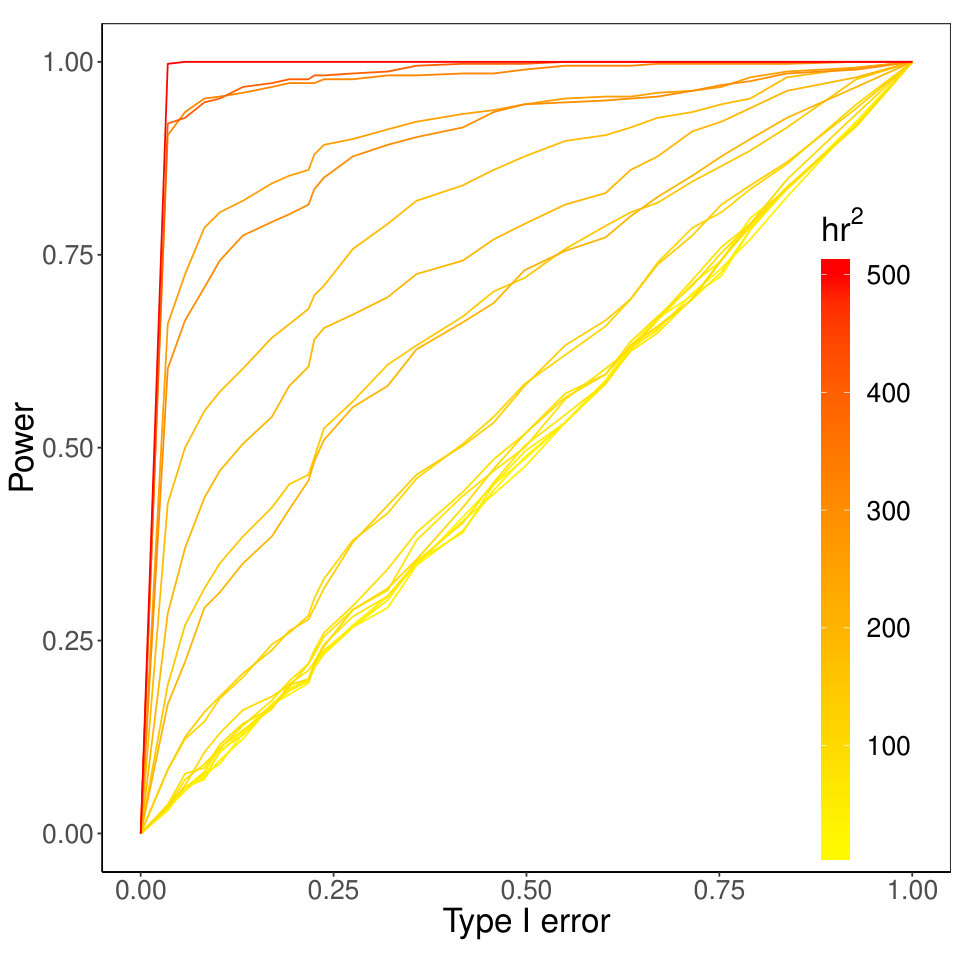
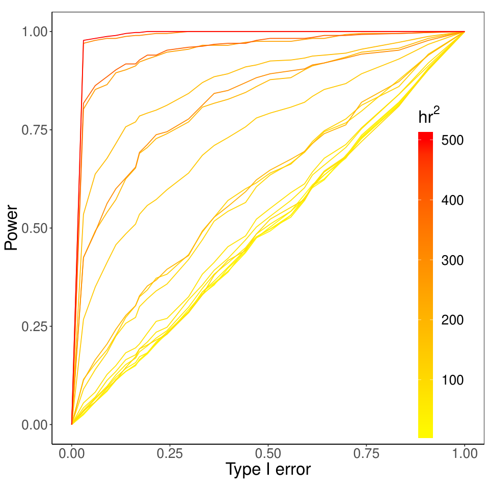
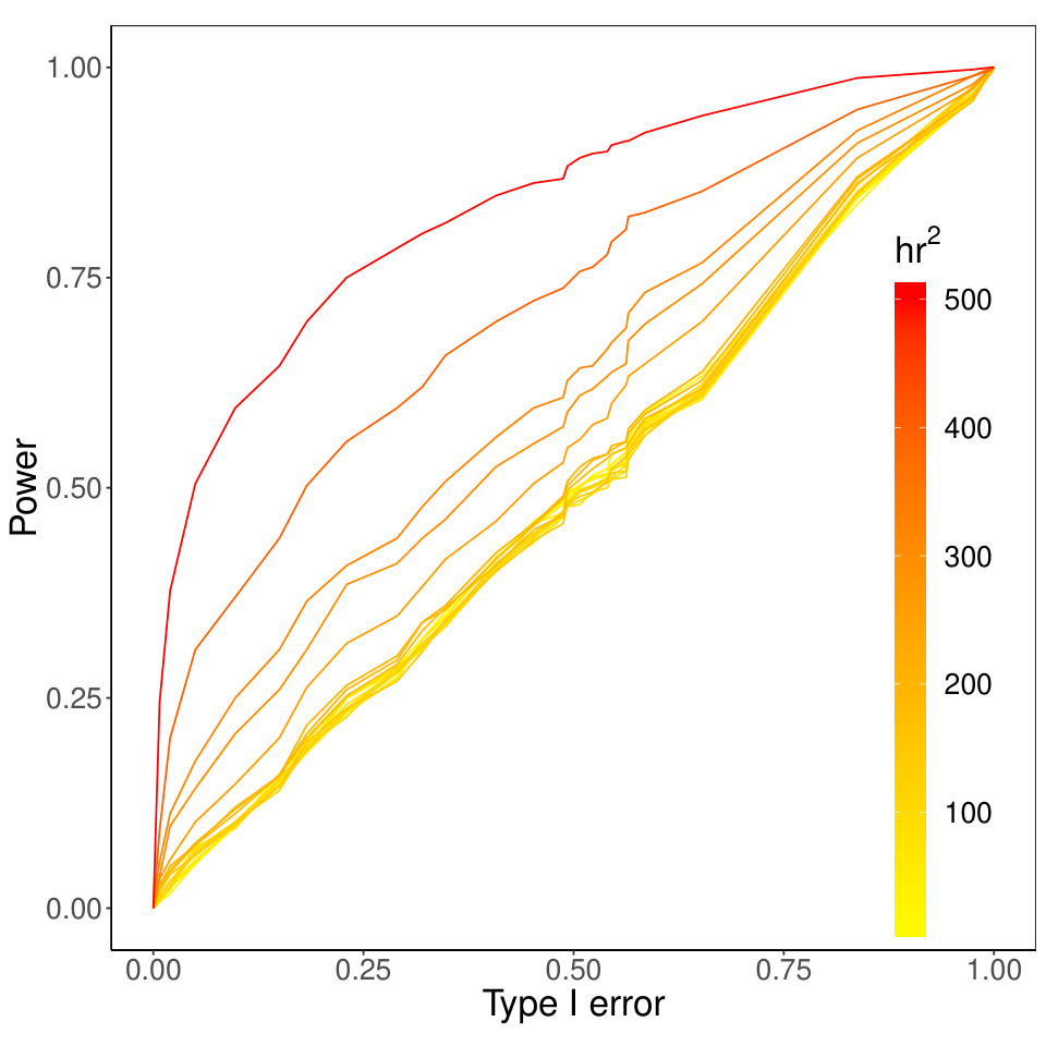
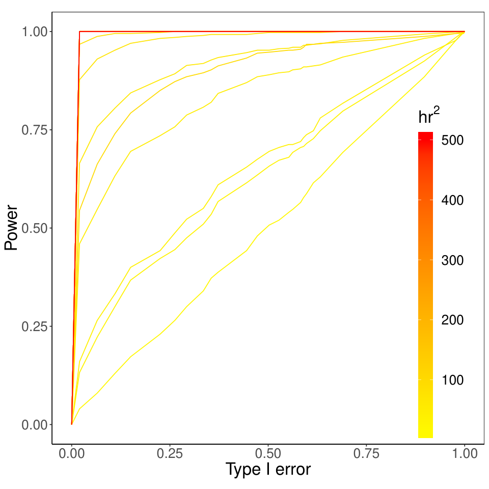
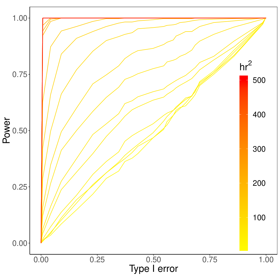
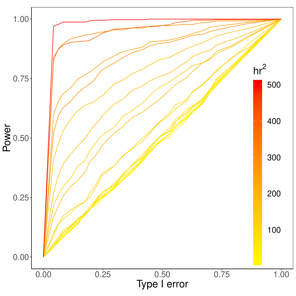
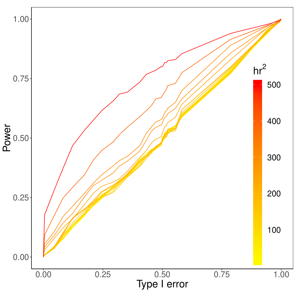
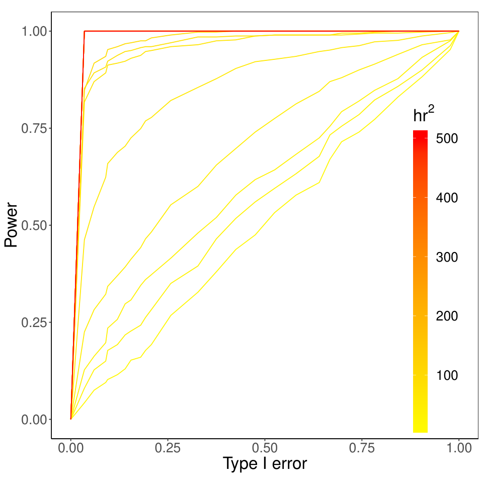
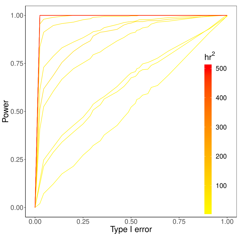
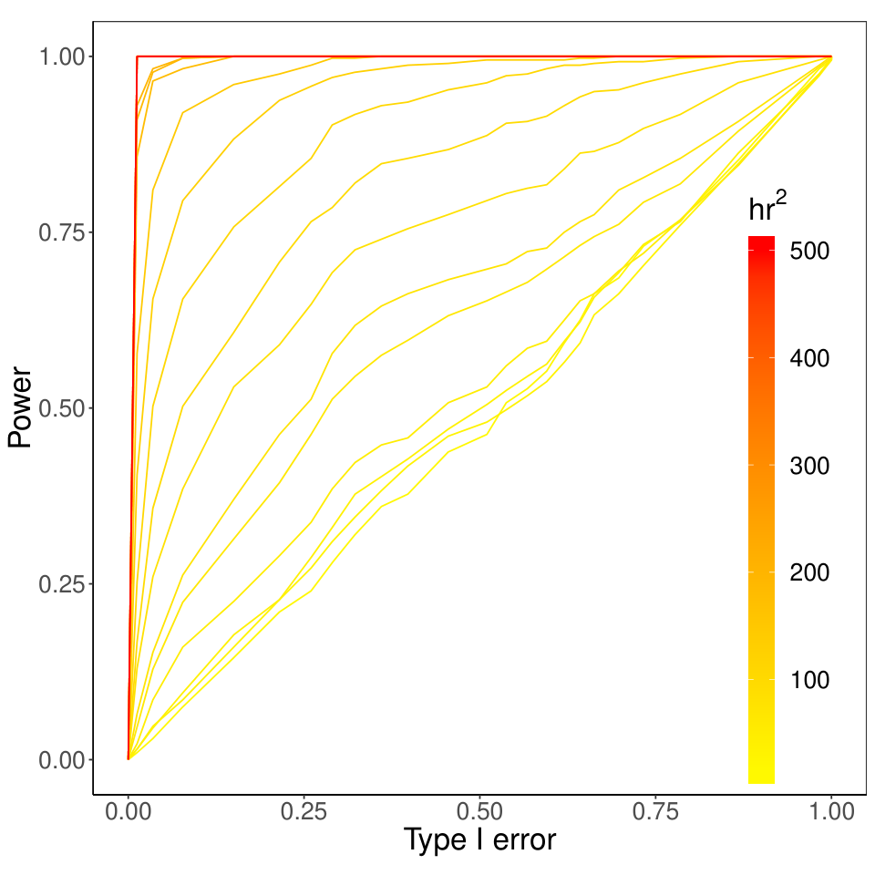
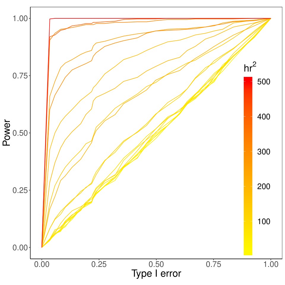
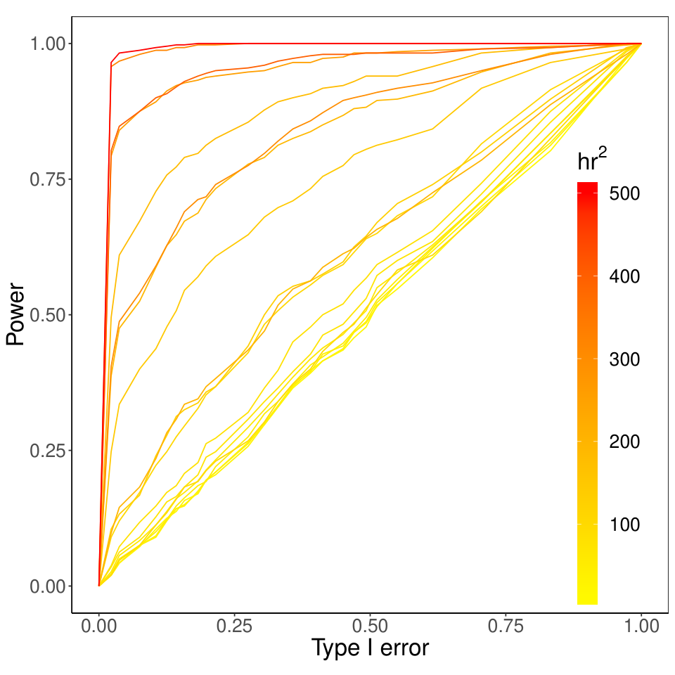
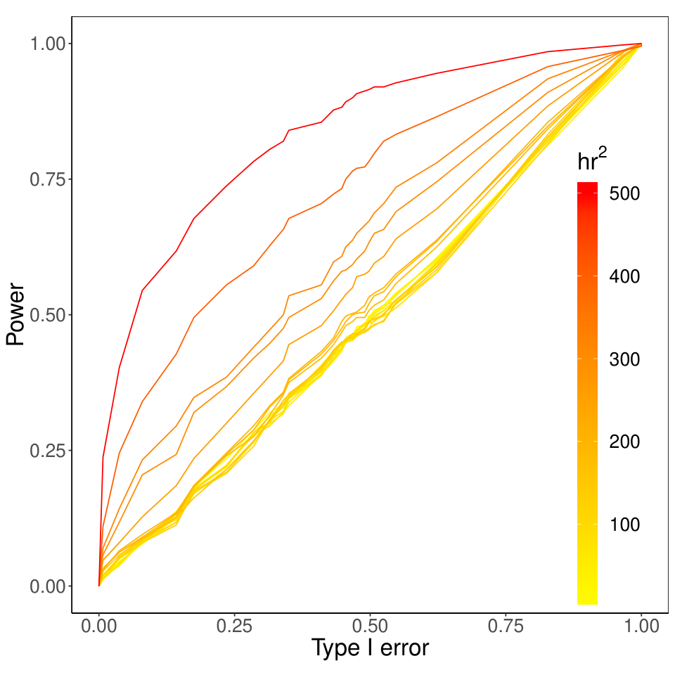
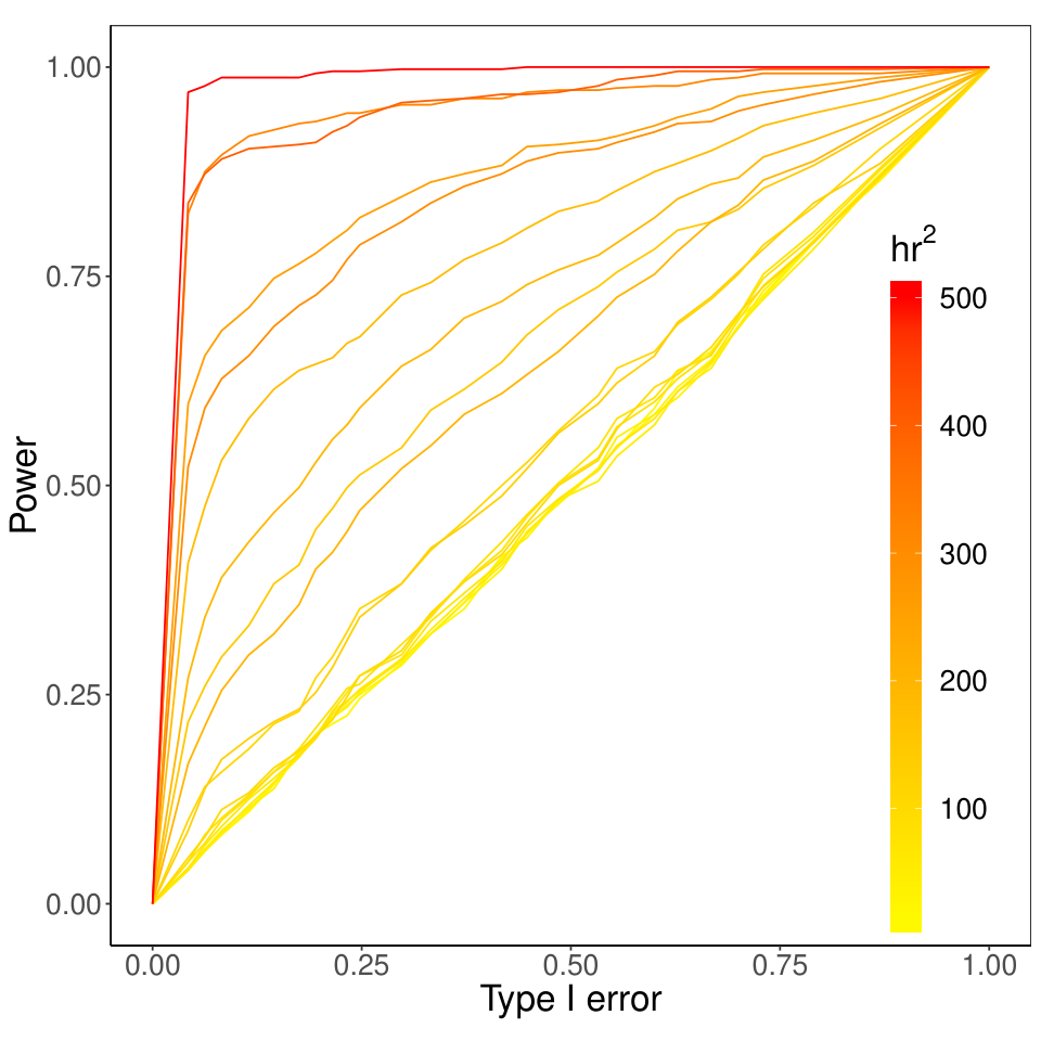
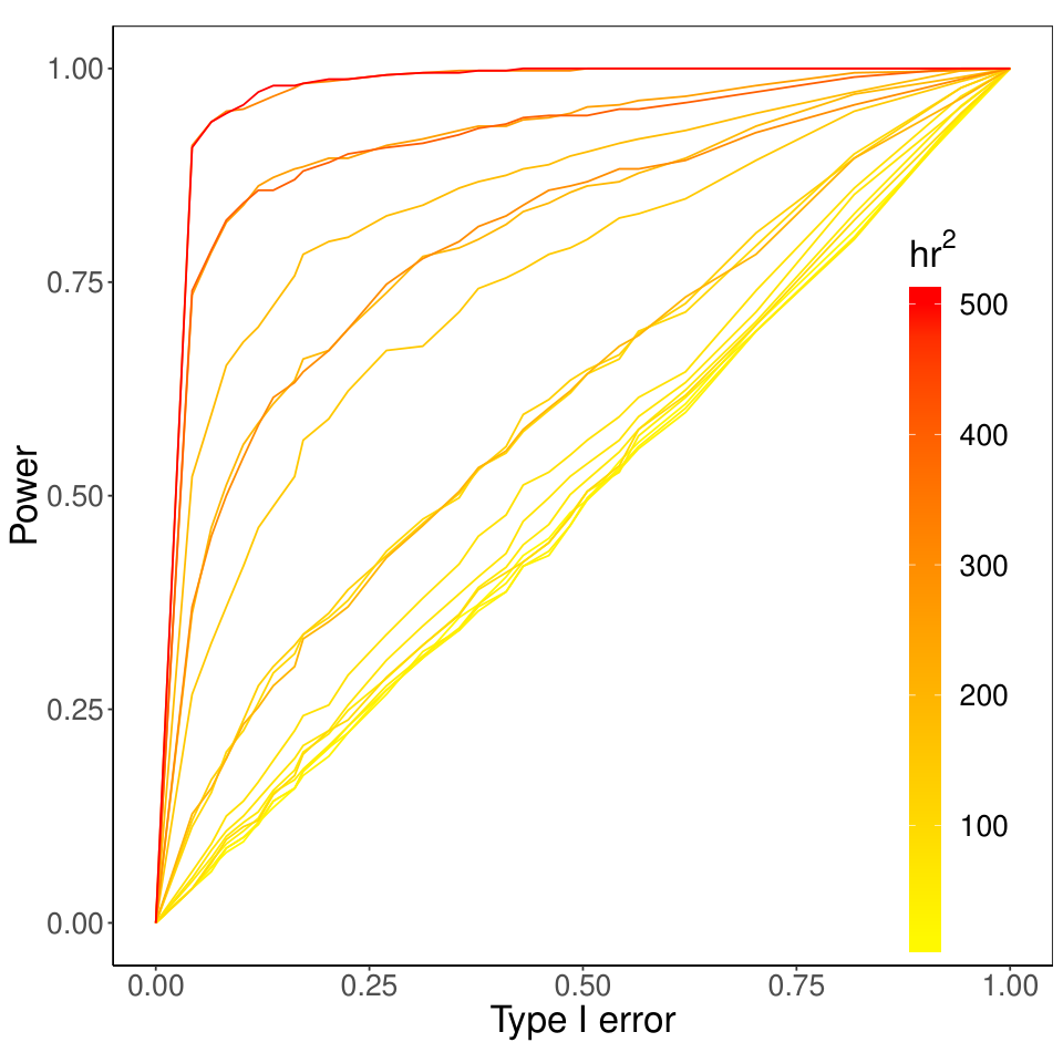
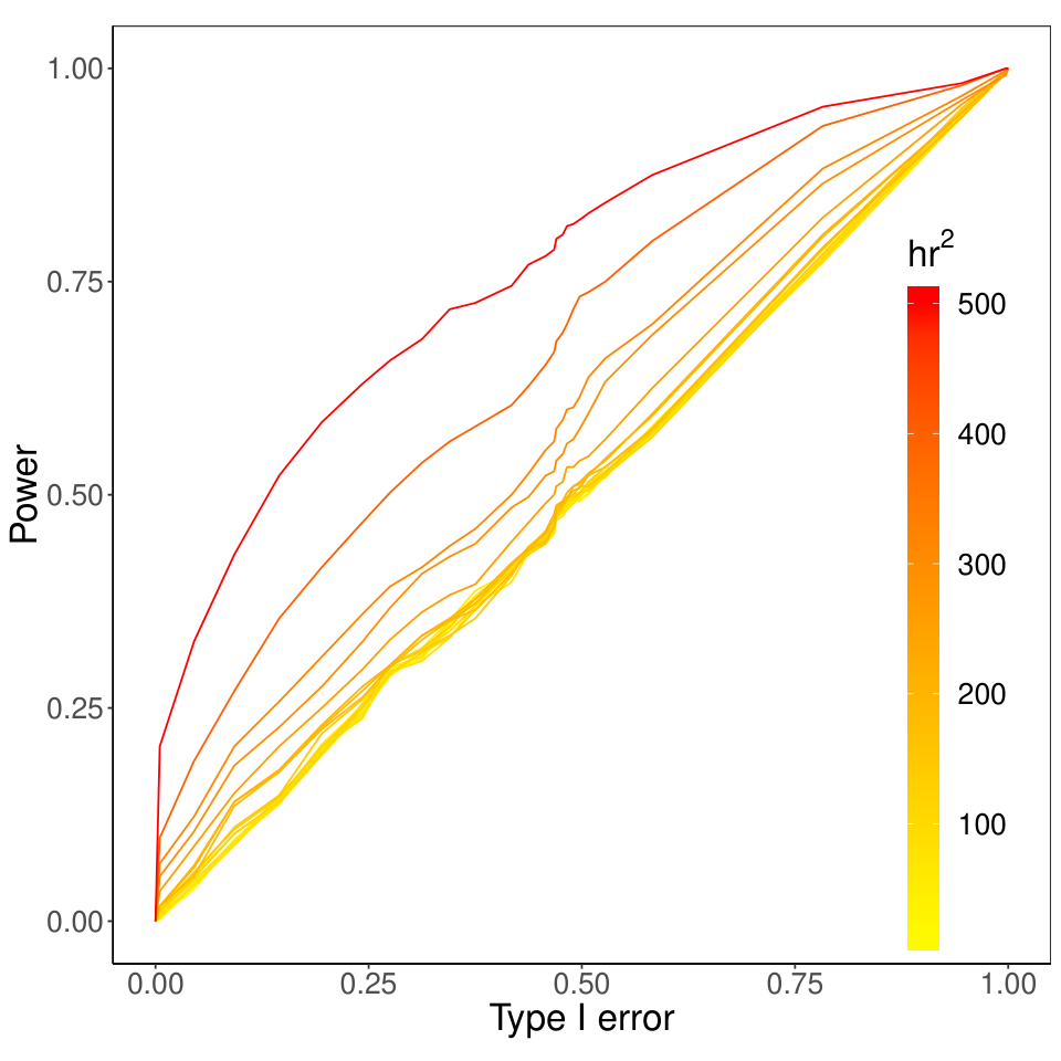
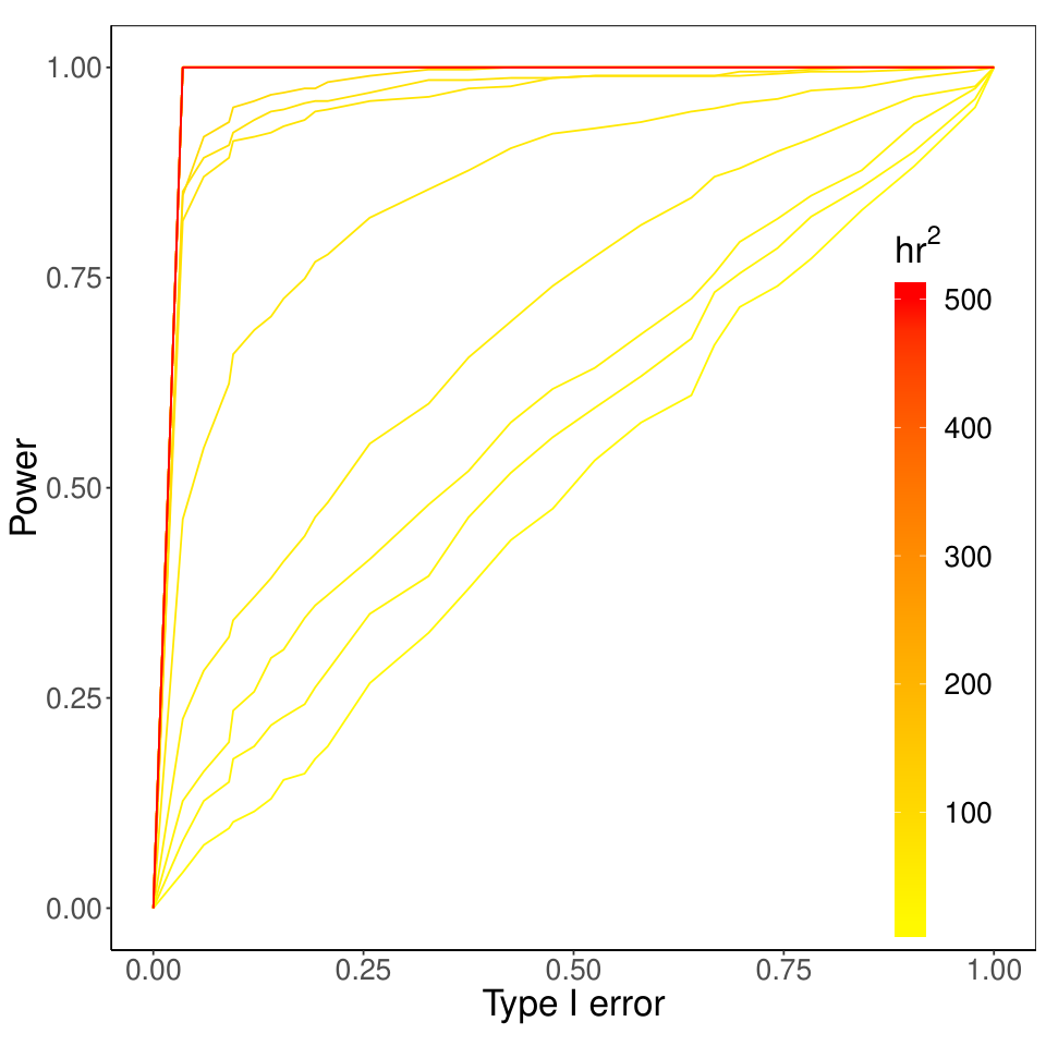
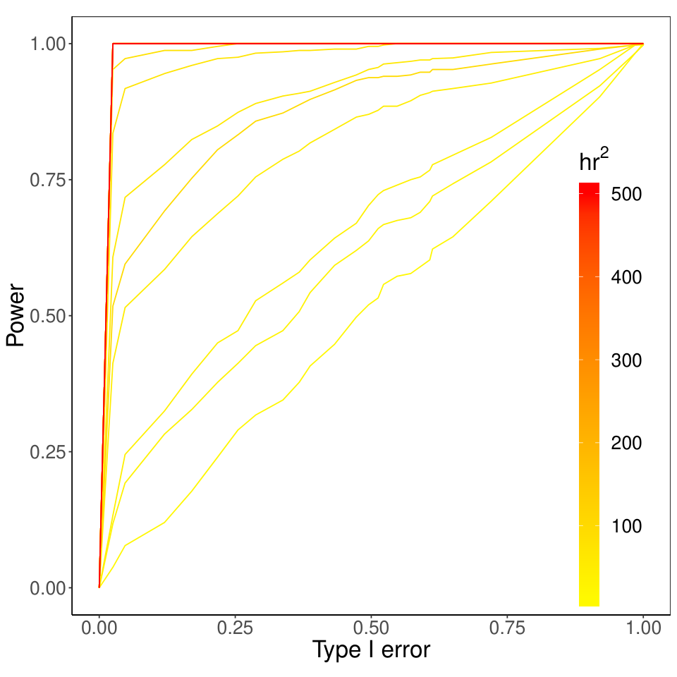
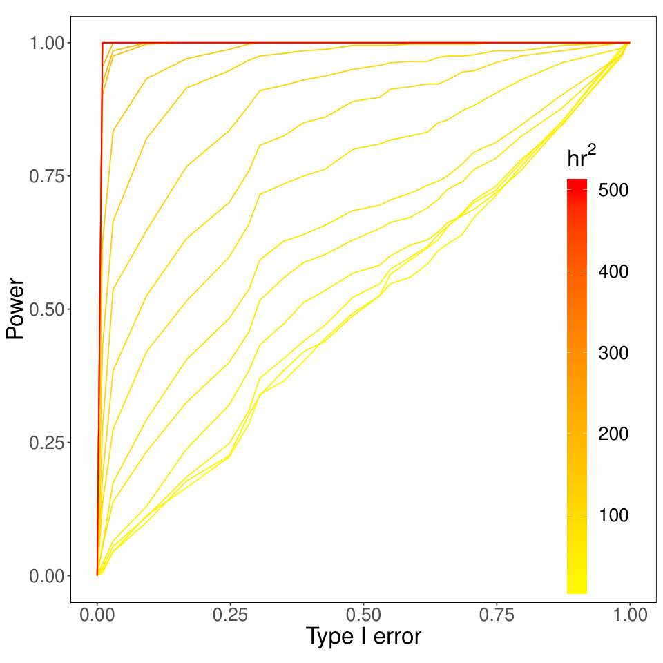
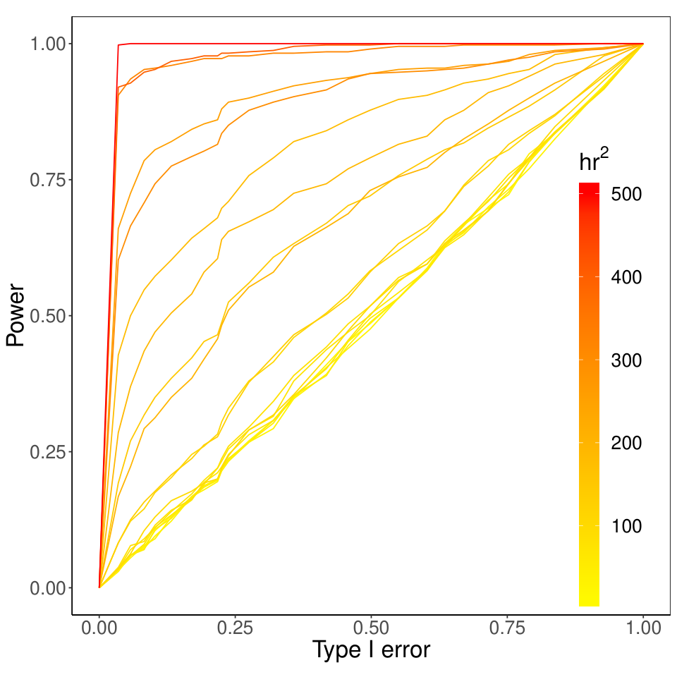
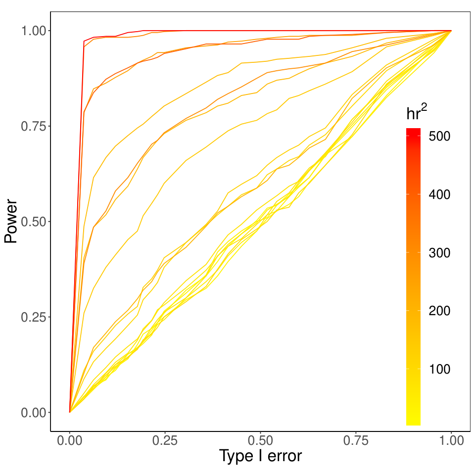
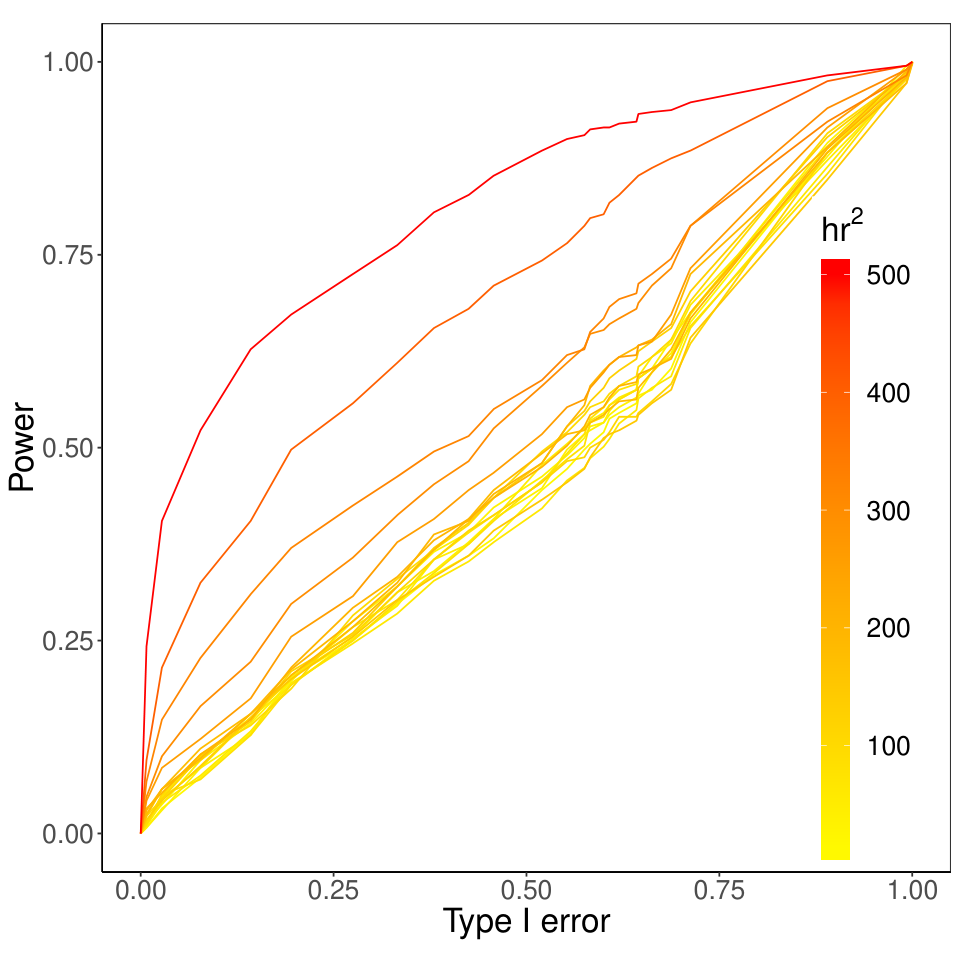
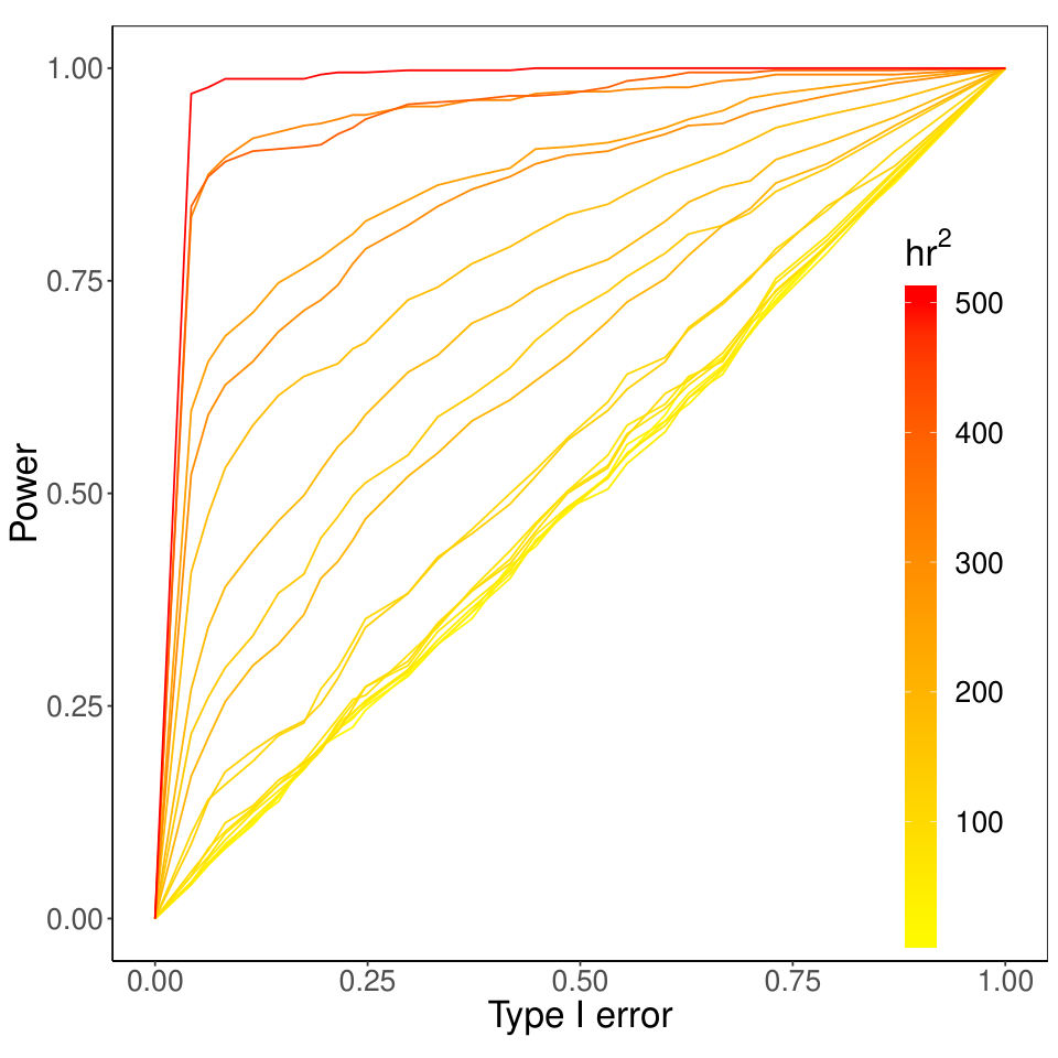
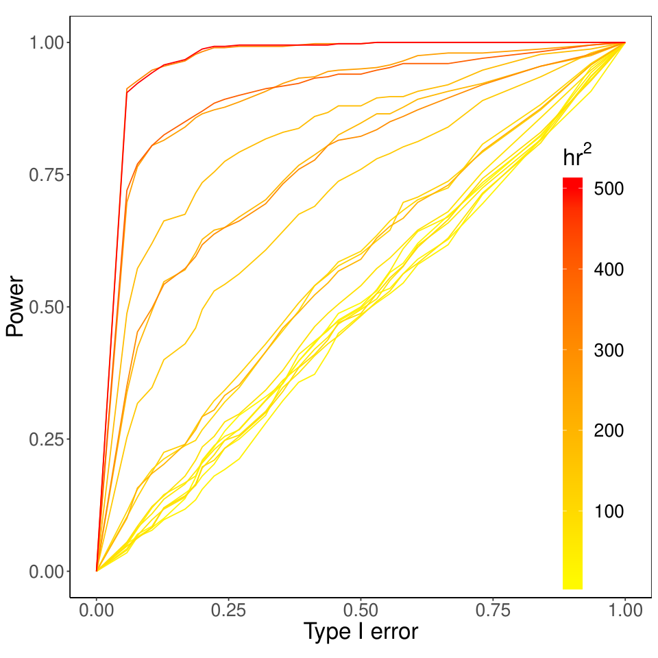
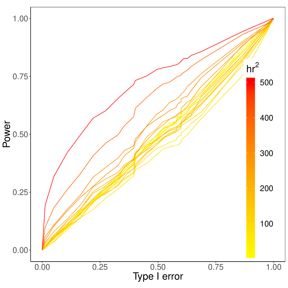
We also used the receiver operating characteristic (ROC) curve (e.g., Egan, 1975) to facilitate comparison of the different methods. Figure 5 shows empirical ROC curves with signals of various volumes, , obtained from the 24 combinations of and in (24), and . Each empirical ROC curve was computed based on 200 images of , 100 of these images generated under the null hypothesis of no signal and the other 100 images generated under the alternative hypothesis by adding a signal given by and in (24). Each curve was traced out by varying on the right-hand side of (23). From Figure 5, we see that the area under the curve (AUC) tends to increase with the signal volume and decrease with the amount of aggregation, as expected. The full set of ROC curves for this experiment is shown in Figure S7 in the Supplementary Material.
| IDL () | CPL () | CPL () |
|---|---|---|
 |
 |
 |
3.2 Experiment 2: Missing data (in a contiguous block) at different scales of aggregation
Experiment 2 is similar to Experiment 1, except that here we considered missing data in the upper-right corner of (), , and , with the fraction of missing data fixed at ; see Figure 6 for an illustration. Tests were carried out at the usual significance level. The empirical power curves and the empirical ROC curves obtained were similar to those in Figures 4 and 5, respectively; for the full set of curves, see Figures S5 and S8 in the Supplementary Material. The results demonstrate that our proposed procedure is not likely to be affected by a large contiguous block of missing data (as long as the block does not contain signal).
| | |
3.3 Experiment 3: Missing data (at random) at different scales of aggregation
Experiment 3 is similar to Experiment 2, except that we considered small blocks missing at random, with the same fraction missing (); see Figure 7 for an illustration. These were taken at random from all blocks except those in the central square region (where the signal is located), shown with a black square outline in each panel of Figure 7. The empirical power curves and the empirical ROC curves obtained were similar to those in Experiments 1 and 2; for the full set of curves, see Figures S6 and S9 in the Supplementary Material. A comparison of Experiments 2 and 3 shows that our proposed procedure, CPL, performs well irrespective of whether the data are missing at random or in a contiguous block. This is an illustration of how spatial modeling and its corresponding conditional simulation can successfully borrow strength for two very different missing-data mechanisms.
| | |
3.4 Experiment 4: Nonstationary noise
Experiment 4 is similar to Experiment 1 except that data are generated with in (4) replaced by a nonstationary process obtained by deforming the coordinates of :
where is a parameter controlling the degree of nonstationarity with corresponding to a non-deformed stationary process. The spatial covariance function of is
A larger departure of from indicates a higher degree of nonstationarity. In this experiment, we considered , , , and . Figure 8 shows five randomly generated datasets with signal magnitude , for . We can see that the data show higher spatial dependence around the upper right-hand corner than the lower left-hand corner for and . In contrast, the data show higher spatial dependence around the lower left-hand corner than the upper right-hand corner for and .
| | | | | |
The empirical power curves for are shown in Figure 9, where the curves are a function of , and . Note that the plot for is the same as the plot for and in Figure 4. Although both IDL and CPL (for ) show elevated Type-I error rates for and , the five plots in Figure 9 generally have similar power curves, indicating that our proposed procedure is robust to mild nonstationarity. Nevertheless, if the nonstationarity is strong (e.g., the variance of varies substantially as ranges over ), then it would not be possible to distinguish the mean from the random component without further prior knowledge on the covariance function.
| | | | | |
4 Applications
4.1 An application to temperature data in the Asia-Pacific
Finding signals in climate data is critically important for assessing the sustainability of Earth’s ecosystems. In this section, we apply our proposed procedure to a temperature dataset obtained from the National Center for Atmospheric Research (NCAR) climate system model. The original data comprise monthly averages of 2-meter air temperatures on the Kelvin scale for the period 1980–1999 over the whole globe on equiangular longitude-latitude (about ) grid cells or pixels. It is of interest to know if there is a decadal change in temperature (i.e., whether there is a possible signal) from the 1980s to the 1990s and, if a change has occurred, to identify the magnitudes and locations of the change. Here, we focus on a region of grid cells containing most of the Asia-Pacific from E to E and from S to N. We obtained the data by computing the average monthly temperature in the 1990s for each pixel in , from which we subtracted the corresponding average monthly temperature in the 1980s. The resulting data, , are shown in Figure 10(a).
| | | |
| (a) | (b) | (c) |
| | | |
| (d) | (e) | (f) |
Just as for the simulation experiments in Section 3, we considered scenarios involving complete data at different resolutions and incomplete data at different resolutions. Under the first of three scenarios, we aggregated into and regular grid cells, denoted by and and shown in Figure 10(b) and Figure 10(c), respectively. Under the next two scenarios, data missing in a contiguous block and data missing at random were considered: Initially, we removed a strip of data from , , and to mimic a missing swath commonly seen in satellite data. The resulting data are denoted by , , and , with the same fraction of fine-resolution pixels missing (), and they are shown in Figures 11(a)–(c), respectively. We then randomly removed a further 1/8 of the grid cells from the datasets , , and , respectively. The resulting data, denoted by , , and , respectively, are shown in Figures 12(a)–(c), where it is seen that after removing data on the strip and the random scattering of pixels, we obtain irregular lattice data.
| | | |
| (a) | (b) | (c) |
| | | |
| (d) | (e) | (f) |
| | | |
| (a) | (b) | (c) |
| | | |
| (d) | (e) | (f) |
We applied the EFDR-CS procedure (with CPL defined in Section 2), based on the significance test (23), to the nine cases of incomplete spatially aggregated data: , , , , , , , , and . Similar to the numerical experiments in Section 3, we used the R package “EFDR" (Zammit-Mangion and Huang, 2015) with its default setting of the Daubechies least asymmetric wavelet filter of length and the number of hypotheses to be tested in the wavelet space fixed at . As for the simulations in Section 3, we chose two wavelet scales resulting in seven wavelet classes corresponding to different scales and orientations. We estimated through (S4) in the Supplementary Material, where and are the ML estimators based on the exponential covariance model, .
Except for the last case, , where one of the missing cells is coincident with the potential signal, our proposed procedure rejected the null hypothesis of no decadal change in temperature at the significance level. The final -values (on the scale ) are shown in Table 1. As expected, for a given row of the Table, the values on the -scale across rows tend to increase (i.e., -values tend to decrease) for data at finer-scale resolutions. Comparison down columns supports our conclusion from the simulations in Section 3, that CPL is not greatly affected by incomplete data as long as the signal is observed.
The spatial patterns of temperature changes, given by in (10) and based on , , , are shown in Figures 10(d)–(f), respectively. As we saw in the simulations in Section 3, our proposed procedure handles successive spatial aggregations well, and very similar signals of temperature increase are observed over central eastern Australia. For the incomplete data, , , , , and , our proposed procedure identified similar signals, albeit with smaller spatial extents. The results are shown in Figures 11(d)–(f) and Figures 12(d)–(e), respectively. However, Figure 12(f) does not show a signal because in , one of the missing cells was coincident with the potential signal (see Figure 12(c)). This resulted in a failure to reject the null hypothesis and an almost blank image in Figure 12(f) with a final -value of that indicates no signal is present. When that cell was allowed to remain and a different cell removed from the dataset in Figure 12(c), went from to , and a spatial signal like those seen in Figures 12(d) and 12(e) appeared.
| Missing Fraction | Scales of Aggregation | ||
|---|---|---|---|
Note: .
4.2 Total column CO2 signal from remote sensing data
We applied the EFDR-CS procedure to a total-column carbon-dioxide (CO2) dataset obtained from the Orbiting Carbon Observatory-2 (OCO-2) satellite of the U.S. National Aeronautics and Space Administration (NASA). The data consist of retrievals measured in parts per million (ppm) during 1–16 July 2018 in a region centered on the Middle East. The retrieval locations and are shown in Figure 13, and the daily retrieval times play a role, as we now explain.
First, we estimated a temporal trend:
and obtained the residuals,
which we now treat as a purely spatial process. Second, a spatial trend that is linear in latitude, , was observed, estimated by ordinary least squares, and subtracted to obtain spatial residuals that now have mean zero:
The residuals are shown in Figure 13; notice that there are large gaps in the map caused by the orbit tracks or no retrieval from the OCO-2 satellite. Third, we obtained the data at the EFDR-CS procedure’s finest resolution by aggregating into longitude-latitude grid cells using simple averaging. We focused on a region from E to E and from N to N (a region of the Middle East, Afghanistan, and the western part of Pakistan), which consists of grid cells at resolution. There were 1548 grid cells out of that contained no data. The resulting data, , consisting of observations, are shown in Figure 14(a), where the 1548 missing data are shown in yellow, and the missing fraction is .

| (a) | (b) |
We applied our EFDR-CS procedure with CPL (defined in Section 2) based on the significance test (23) in the same way as in Section 4.1. We estimated through (S4) in the Supplementary Material, but now , , and are ML estimators based on the exponential covariance model with a nugget effect (i.e., ) to account for fine-scale-process variability. The estimated map of the signal is displayed in Figure 14(b), which shows a large hotspot in west Pakistan in the vicinity of Karachi, of about +4ppm. Our inference on rejected the null hypothesis : at the 5 significance level with a -value of , indicating that the signal is real.
5 Discussion and conclusions
In this article, we have proposed a spatial inference procedure to detect signals from possibly incomplete, area-aggregated data, in the presence of spatially correlated noise. The procedure, which we call EFDR-CS, is based on using the Enhanced False Discovery Rate and Conditional Simulations to infer the fine-scale spatial signal from incomplete spatially aggregated data.
A critical component of the research presented in this article is a novel methodology to combine exchangeable -values into a single -value using a bivariate Gaussian copula and a composite likelihood. In Section 3 and the Supplementary Material, we show that the methodology is able to properly control the Type-I error rate, even when the -values are strongly correlated. Further, we can extend the rectangular dimensions and to their next powers of two, to deal with any boundary effects caused by applying a DWT to a rectangular image.
While we consider that the image at the original pixel resolution follows a multivariate Gaussian distribution, it is possible to extend the CS approach for images generated from non-Gaussian distributions (or even discrete distributions). For example, one might use a generalized linear mixed model for non-Gaussian data, with the random effects derived from a latent Gaussian spatial process (e.g., Sengupta et al., 2016; Wilson and Wakefield, 2020). This would be useful when, for example, are counts of events aggregated over a number of regions from a log-Gaussian Cox process. It would be straightforward to adapt the procedure proposed in this paper to these models by defining the signal to be the mean of the latent Gaussian process. The null hypothesis, : , could be tested by conditionally simulating the hidden Gaussian process times, conditional on the data. Then EFDR would be applied to each simulated process and the resulting -values combined into a single -value, as we have done for Gaussian data.
Acknowledgments
Hsin-Cheng Huang’s research was supported by ROC Ministry of Science and Technology grants MOST 105-2119-M-007-032 and MOST 106-2118-M-001-002-MY3. Noel Cressie’s research was supported by Australian Research Council Discovery Projects DP150104576 and DP190100180, and by NSF grant SES-1132031 funded through the NSF-Census Research Network (NCRN) program. Andrew Zammit-Mangion’s research was supported by Australian Research Council Discovery Early Career Research Award (DECRA) DE180100203 and Discovery Project DP190100180. Cressie’s and Zammit-Mangion’s research was also supported by NASA ROSES grant 17-OCO2-17-0012. The authors would like to thank Chris Wikle, Scott Holan, Vineet Yadav, and Mike Gunson for comments on parts of this research, and Yi Cao for assistance with Section 4.2.
Supplementary Material
The supplementary material consists of three sections. Section S1 gives estimation of the spatial covariance parameters introduced in Section 2.2. Section S2 provides an initial simulation study to investigate the Type-I error rates obtained using the testing rule (23). Section S3 contains complete figures for the simulations in Section 3. These include: and , corresponding to in Figure 2; empirical power curves as a function of the signal’s magnitude , for various procedures (NVE, IDL, our proposed procedure CPL, and its variant MOM); and empirical ROC curves for CPL, where the signal volume is varied.
References
-
Benjamini, Y. and Heller, R. (2007). False discovery rates for spatial signals. Journal of the American Statistical Association, 102, 1272-1281.
-
Benjamini, Y. and Hochberg, Y. (1995). Controlling the false discovery rate: A practical and powerful approach to multiple testing, Journal of the Royal Statistical Society, Series B, 57, 289-300.
-
Brown, M. (1975). A method for combining non-independent, one-sided tests of significance, Biometrics, 31, 987-992.
-
Cressie, N. (1993). Statistics for Spatial Data, rev. edn, Wiley, New York, NY.
-
Daubechies, I. (1992). Ten Lectures on Wavelets, CBMS-NSF Regional Conference Series in Applied Mathematics, SIAM, Philadelphia, PA.
-
Egan, J. P. (1975). Signal Detection Theory and ROC Analysis, Academic Press, New York, NY.
-
Fisher, R. A. (1925). Statistical Methods for Research Workers, Oliver and Boyd, Edinburgh, UK.
-
Gilleland, E. (2013). Testing competing precipitation forecasts accurately and efficiently: The spatial prediction comparison test, Monthly Weather Review, 141, 340-355.
-
Hering, A. S. and Genton, M. G. (2011). Comparing spatial predictions, Technometrics, 53, 414-425.
-
Lei, L., Ramdas, A., and Fithian, W. (2017). STAR: A general interactive framework for FDR control under structural constraints, arXiv preprint arXiv:1710.02776.
-
Littell, R. C. and Folks, J. L. (1971). Asymptotic optimality of Fisher’s method of combining independent tests, Journal of the American Statistical Association, 66, 802-806.
-
Little, R. J. A. and Rubin, D. B. (2002). Statistical Analysis with Missing Data, 2nd edn, Wiley, New York, NY.
-
Martinez, J. G., Bohn, K. M., Carroll, R. J., and Morris, J. S. (2013). A study of Mexican free-tailed bat chirp syllables: Bayesian functional mixed models for nonstationary acoustic time series, Journal of the American Statistical Association, 108, 514-526.
-
Nguyen, H., Cressie, N., and Braverman, A. (2012). Spatial statistical data fusion for remote sensing applications, Journal of the American Statistical Association, 107, 1004-1018.
-
Risser, M. D., Paciorek, C. J., and Stone, D. A. (2019). Spatially-dependent multiple testing under model misspecification, with application to detection of anthropogenic influence on extreme climate events, Journal of the American Statistical Association, 114, 61-78.
-
Schott, J. R. (2017). Matrix Analysis for Statistics, 3rd edn, Wiley, Hoboken, NJ.
-
Sengupta, A., Cressie, N., Kahn, B. H., and Frey, R. (2016). Predictive inference for big, spatial, non-Gaussian data: MODIS cloud data and its change-of-support, Australian and New Zealand Journal of Statistics, 58, 15-45.
-
Shen, X., Huang, H.-C., and Cressie, N. (2002). Nonparametric hypothesis testing for a spatial signal, Journal of the American Statistical Association, 97, 1122-1140.
-
Song, P. X.-K. (2000). Multivariate dispersion models generated from Gaussian copula, Scandinavian Journal of Statistics, 27, 305-320.
-
Spiegelhalter, D. J., Abrams, K. R., and Myles, J. P. (2004). Bayesian Approaches to Clinical Trials and Health-Care Evaluation, Wiley, New York, NY.
-
Sun, W., Reich, B.J., Cai, T.T., Guindani, M., and Schwartzman, A. (2015). False discovery control in large-scale spatial multiple testing, Journal of the Royal Statistical Society, Series B, 77, 59-83.
-
Wasserstein, R. L., Schirm, A. L., and Lazar, N. A. (2019). Moving to a world beyond “," The American Statistician, 73, 1-19.
-
Wilson, K. and Wakefield, J. (2020). Pointless spatial modeling, Biostatistics, 21, e17-e32.
-
Ye, J. (1998). On measuring and correcting the effects of data mining and model selection, Journal of the American Statistical Association, 93, 120-131.
-
Yekutieli, D and Benjamini, Y. (1999). Resampling-based false discovery rate controlling multiple test procedures for correlated test statistics, Journal of Statistical Planning and Inference, 82, 171-196.
-
Yun, S., Zhang, X., and Li, B. (2018). Detection of local differences between two spatiotemporal random fields, Manuscript.
-
Zammit-Mangion, A. and Huang, H.-C. (2015). EFDR: Wavelet-based enhanced FDR for signal detection in noisy images, R package version 0.1.1. URL https://CRAN.R-project.org/package=EFDR.
Supplementary Material for “False Discovery Rates to Detect Signals from Incomplete Spatially Aggregated Data"
The supplementary material consists of three sections. Section S1 gives estimation of introduced in Section 2.2. Section S2 provides an initial simulation study to investigate the Type-I error rates obtained using the significance test (23). Section S3 contains nine figures for the simulations in Section 3.
S1 Estimation of spatial dependence from incomplete spatially aggregated data
To obtain in Section 2.2, we start with the null hypothesis in (2) and a model in the wavelet domain for defined by (7). As in Shen et al. (2002), the wavelet coefficients, , are modeled independently as
| (S1) |
The covariance matrix in the wavelet domain, is a diagonal matrix whose -th diagonal block is given by , for . We estimate through
| (S2) |
since is orthogonal. In (S2), is the Frobenius norm and is a smooth empirical estimator, here the maximum likelihood (ML) estimator of under a parametric covariance model, , and . Note that it is generally not possible to define the usual method-of-moments estimator of from the incomplete spatially aggregated data , for which there are no replications available.
As an example, consider the Matérn covariance model for given by,
| (S3) |
where is the modified Bessel function of the second kind of order , is a variance parameter, and consists of a spatial-scale parameter , a smoothness parameter , and a nugget-effect parameter . Under , the ML estimator of can be obtained from the data, , by minimizing the negative log profile likelihood, as follows:
where is an correlation matrix whose -th entry is . Then the ML estimator of the stationary variance is:
Consequently, a smooth empirical estimator of for use in (S2) is given by .
Let be a sub-matrix of , consisting of the rows corresponding to the -th wavelet component. Then . It follows from (S2) that is given by,
| (S4) |
where is the number of rows of , and denotes the trace of a square matrix .
S2 Observed Type-I error rates using -values from correlated -tests
We conducted an initial simulation study to investigate the Type-I error rates obtained using the significance test (23) when the level of exchangeability was estimated using copulas (CPL) and the method-of-moments (MOM). The significance test where the -values are combined naïvely through their simple average (NVE) was also considered for comparison. In this study, the -values came from a two-sided -test for the mean of a Gaussian distribution with known variance; the purpose of the study is to assess the validity of our proposed procedure in a very simple, non-spatial setting where there is exchangeability.
Let the set be made up of elements distributed independently as , for . We put and drew from , and then we randomly drew subsamples of size without replacement from . For , let be the -th subsample and be a statistic for testing the hypotheses, versus . Under , it is easy to see that and . However, the are dependent; indeed, they are exchangeable due to the sampling-without-replacement from .
The individual -test, based on the statistic , rejects if
| (S5) |
where is a pre-specified significance level. Because are exchangeable, so too are the -values . We are interested in knowing how well they can be combined into a single -value using the naïve procedure of averaging (NVE), our proposed copula-based procedure (CPL), and its method-of-moments variant (MOM). That is, we compare
Note that a Type-I error occurs if, under , the resulting -value is smaller than .
In this experimental set-up, the level of exchangeability in the intra-class correlation model (12) is higher when (i.e., the subsample size) is closer to the full sample size of . So we considered only . In addition, we considered the three significance levels, , commonly used in practice. The resulting empirical Type-I error rates for the three methods (NVE, CPL, MOM) under the 12 different combinations of and , based on 50,000 simulation replicates, are shown in Table S1.
| NVE | CPL | MOM | ||
|---|---|---|---|---|
| 0.01 | 80 | 0.0016 (0.0002) | 0.0078 (0.0004) | 0.0063 (0.0004) |
| 85 | 0.0030 (0.0002) | 0.0089 (0.0004) | 0.0073 (0.0004) | |
| 90 | 0.0049 (0.0003) | 0.0098 (0.0004) | 0.0087 (0.0004) | |
| 95 | 0.0065 (0.0004) | 0.0098 (0.0004) | 0.0090 (0.0004) | |
| 0.05 | 80 | 0.0161 (0.0006) | 0.0454 (0.0009) | 0.0446 (0.0009) |
| 85 | 0.0233 (0.0007) | 0.0488 (0.0010) | 0.0481 (0.0010) | |
| 90 | 0.0305 (0.0008) | 0.0482 (0.0010) | 0.0478 (0.0010) | |
| 95 | 0.0389 (0.0009) | 0.0485 (0.0010) | 0.0482 (0.0010) | |
| 0.10 | 80 | 0.0443 (0.0009) | 0.0958 (0.0013) | 0.1033 (0.0014) |
| 85 | 0.0574 (0.0010) | 0.0968 (0.0013) | 0.1044 (0.0014) | |
| 90 | 0.0686 (0.0011) | 0.0949 (0.0013) | 0.1001 (0.0013) | |
| 95 | 0.0828 (0.0012) | 0.0971 (0.0013) | 0.0997 (0.0013) |
NVE consistently gives Type-I error rates that are too small, which was expected since the sample average of the -values results in a combined -value that tends to be too large, causing the null hypothesis to be rejected less often than it should. The effect is less pronounced when the -values are more correlated; that is, as the size of the subsample increases, the Type-I error rate of NVE improves. Our proposed procedure, whether it is CPL or MOM, is adaptive to the amount of dependence, and the Type-I error rates are very close to the nominal levels for all cases.
This initial study is encouraging and indicates that our proposal is valid in the presence of exchangeably dependent -values.
S3 Figures for the simulations in Section 3
This section contains the following nine figures:
- S1
Images of with and signals from (24) of various extents down rows and various magnitudes across columns.
- S2
Images of obtained by aggregating in Figure S1 into blocks resulting in grid cells.
- S3
Images of obtained by aggregating in Figure S1 into blocks resulting in grid cells.
- S4–S6
Empirical power curves as a function of the signal’s magnitude , for various procedures for testing of in Experiments 1–3 in Section 3, respectively.
- S7–S9
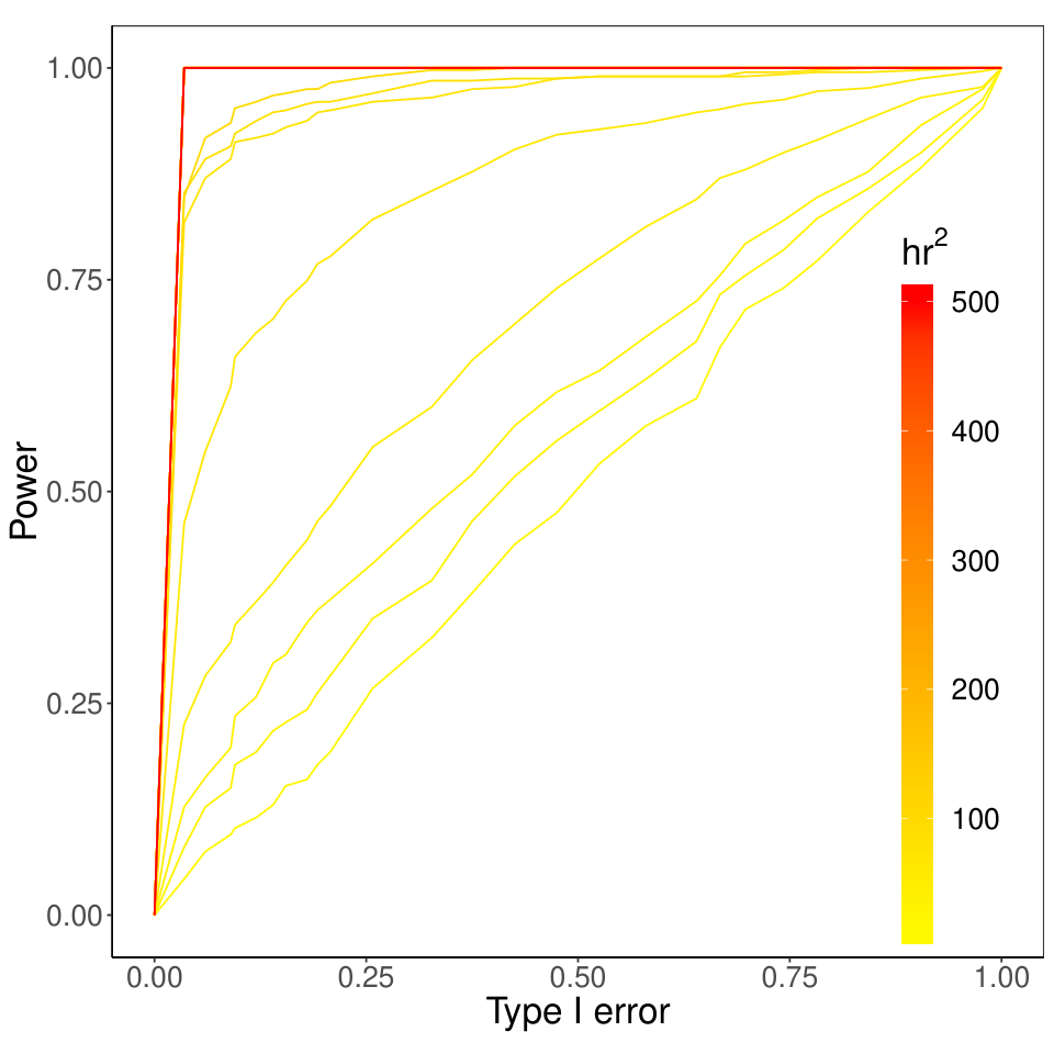
Empirical ROC curves for IDL and the proposed procedure, CPL, in Experiments 1–3 in Section 3, respectively.
|
|
| | | | |
|
|
| | | | |
|
|
| | | | |
|
|
| | | | |
|
|
| | | | |
|
|
| | | | |
|
|
| | | | |
|
|
| | | | |
|
|
| | | | |
|
|
| | | | |
|
|
| | | | |
|
|
| | | | |
|
|
||
|---|---|---|
|
|
||
|
|
||
|
|
|
|
||
|---|---|---|
|
|
||
|
|
||
|
|
|
|
||
|---|---|---|
|
|
||
|
|
||
|
|
| IDL | CPL () | CPL () |
|---|---|---|
 |
 |
 |
 |
 |
 |
 |
 |
 |
| CPL () | CPL () | CPL () |
|---|---|---|
 |
 |
 |
 |
 |
 |
 |
 |
 |
| CPL () | CPL () | CPL () |
|---|---|---|
 |
 |
 |
 |
 |
 |
 |
 |
 |