Stochastic approximation with cone-contractive operators: Sharper -bounds for -learning
| Martin J. Wainwright (GD) |
| Departments of Statistics and EECS |
| UC Berkeley |
| Voleon Group, Berkeley, CA |
| wainwrig@berkeley.edu |
Abstract
Motivated by the study of -learning algorithms in reinforcement learning, we study a class of stochastic approximation procedures based on operators that satisfy monotonicity and quasi-contractivity conditions with respect to an underlying cone. We prove a general sandwich relation on the iterate error at each time, and use it to derive non-asymptotic bounds on the error in terms of a cone-induced gauge norm. These results are derived within a deterministic framework, requiring no assumptions on the noise. We illustrate these general bounds in application to synchronous -learning for discounted Markov decision processes with discrete state-action spaces, in particular by deriving non-asymptotic bounds on the -norm for a range of stepsizes. These results are the sharpest known to date, and we show via simulation that the dependence of our bounds cannot be improved in any uniform way. These results show that relative to model-based -iteration, the -based sample complexity of -learning is suboptimal in terms of the discount factor .
1 Introduction
Stochastic approximation (SA) algorithms are widely used in many areas, including stochastic control, communications, machine learning, statistical signal processing and reinforcement learning, among others. There is now a very rich literature on SA algorithms, their applications and the associated theory (e.g., see the books [5, 13, 8] and references therein). One set of fundamental questions concerns the convergence of SA algorithms; there are various general techniques for establishing convergence, including the ODE method, dynamical system, and Lyapunov-based methods, among others. Much of the classical theory in stochastic approximation is asymptotic in nature, whereas in more recent work, particularly in the special case of stochastic optimization, attention has been shifted to non-asymptotic results [14, 4].
The goal of this paper is to develop some non-asymptotic bounds for a certain class of stochastic approximation procedures. The motivating impetus for this work was to gain a deeper insight into the classical -learning algorithm [25] from Markov decision processes and reinforcement learning [17, 19, 6, 7, 21]. It is a stochastic approximation algorithm for solving a fixed point equation involving the Bellman operator. In the discounted setting, this operator is contractive with respect to a sup norm, and also monotonic in the elementwise ordering. We show that these conditions can be viewed as special cases of a more general structure on the operators used in stochastic approximation for solving fixed point equations. In particular, we introduce monotonicity and quasi-contractivity conditions that are defined with respect to the partial order and gauge norms induced by an underlying cone. In the case of sup norm contractions, this underlying cone is the orthant cone, but other cones also arise naturally in applications. For instance, for SA procedures that operate in the space of symmetric matrices, the cone of positive semidefinite matrices induces the spectral order, as well as various forms of spectral norms. For a sequence of operators satisfying these cone monotonicity and quasi-contractivity conditions, we prove a general result (Theorem 1) that sandwiches the error at each iteration in terms of the partial order induced by the cone. By considering concrete choices of stepsize—such as linearly or polynomial decaying ones—we derive corollaries that yield non-asymptotic bounds on the error.
We specialize this general theory to the synchronous form of -learning in discounted Markov decision processes, and use it to derive non-asymptotic bounds on the -error of -learning, for both polynomial stepsizes and a linearly rescaled stepsize. Notably, these results are the sharpest known to date, and depend on the structure of the optimal -function. We show via simulation studies that our bounds are unimprovable in general. In particular, we exhibit a “hard” problem for which our theory predicts that the number of iterations required to obtain an -accurate solution in -norm should scale as , and show that this prediction is empirically sharp. In the the worst case setting, our bounds lead to scaling, a scaling that matches known bounds on synchronous -learning from previous work [10]; however, we are not aware of a problem for which this worst-case bound is actually sharp. For context, we note that the speedy-Q-learning method, an extension of ordinary -learning, is known to have iteration complexity scaling as . Moreover, Azar et al. [3] show that model-based -iteration exhibits a scaling, and moreover that this is the best possible for any method in a minimax sense. Consequently, a corollary of our results is to reveal a gap between the performance of standard synchronous -learning and an optimal (model-based) procedure.
The remainder of this paper is organized as follows. In Section 2, we introduce the class of stochastic approximation algorithms analyzed in this paper, including some required background on cones and induced gauge norms. We then state our main result (Theorem 1), as well some of its corollaries for particular stepsize choices (Corollaries 1 and 2). In Section 3, we turn to the analysis of -learning. After introducing the necessary background in Section 3.1, we then devote Section 3.2 to statement of our two main results on -learning, namely -norm bounds for a linear rescaled stepsize (Corollary 3) and for polynomially decaying stepsizes (Corollary 4). In Section 3.3, we discuss past work on -learning and compare our guarantees to the best previously known non-asymptotic results. In Section 3.4, we describe and report the results of a simulation study that provides empirical evidence for the sharpness of our bounds. We conclude with a discussion in Section 4, with more technical aspects of our proofs deferred to the appendices.
2 A general convergence result
In this section, we set up the stochastic approximation algorithms of interest. Doing so requires some background on cones, monotonic operators on cones, and gauge norms induced by order intervals, which we provide in Section 2.1. In Section 2.2, we state a general result (Theorem 1) that sandwiches the iterate error using the partial order induced by the cone. This result holds for arbitrary stepsizes in the interval ; we follow up by using this general result to derive specific bounds that apply to stepsize choices commonly used in practice (cf. Corollaries 1 and 2).
2.1 Background and problem set-up
Consider a topological vector space , and an operator that maps to itself. Our goal is to compute a fixed point of —that is, an element such that —assuming that such an element exists and is unique. In various applications, we are not able to evaluate exactly, but instead are given access to a sequence of auxiliary operators , and permitted to compute the quantity for any . Here denotes an error term, allowed to be arbitrary in the analysis of this section. In the simplest case, we have for all , but the additional generality afforded by the setup here turns out to be useful.
Given an observation model of this type, we consider algorithms that generate a sequence according to the recursion
| (1) |
The stepsize parameters are assumed to belong to the interval , and should be understood as design parameters. Our primary goals are to specify conditions on the auxiliary operators , noise sequence , and stepsize sequence under which the sequence converges to . Moreover, we seek to develop tools for proving non-asymptotic bounds on the error—i.e., guarantees that hold for finite iterations, as opposed to in the limit as increases to infinity.
Of course, convergence guarantees are not possible without imposing assumptions on the auxiliary operators. In this paper, motivated by the analysis of -learning and related algorithms in reinforcement learning, we assume that they satisfy certain properties that depend on a cone contained in . Let us first introduce some relevant background on cones, order intervals and induced gauge norms. Any cone induces a partial order on via the relation
| (2) |
Cones that have non-empty interiors and are topologically normal [1, 12] can also be used to induce a certain class of gauge norms as follows. For a given element , the associated order interval is the set
| (3a) | ||||
| and it defines the Minkowski (gauge) norm given by | ||||
| (3b) | ||||
Let us consider some concrete examples to illustrate.
Example 1 (Orthant cone and -norms).
Suppose that is the usual Euclidean space d, and consider the orthant cone , where . It induces the usual elementwise ordering—viz. if and only if for all . Setting to be the all-ones vector, we find that
Thus, this choice of induces the usual -norm on vectors. Setting to some other vector contained in the interior of the orthant cone yields a weighted -norm.
Example 2 (Symmetric matrices and spectral norm).
Now suppose that is the space of -dimensional symmetric matrices . Letting denote the eigenvalues of a matrix , consider the cone of positive semidefinite matrices
This cone induces the spectral ordering if and only if all the eigenvalues of are non-negative. Setting to be the identity matrix , we have
so that the induced gauge norm is the spectral norm on symmetric matrices.
In this paper, we assume that the operators in the recursion (1) satisfy two properties: cone-monotonicity and cone-quasi-contractivity. More precisely, we assume that for each , the operator is monotonic with respect to the cone, meaning that
| (4a) | ||||
| Moreover, we assume that for some element , it is cone-quasi-contractive meaning that there is some and some such that | ||||
| (4b) | ||||
Here the terminology “quasi” denotes the fact that the relation (4b) only need hold for a single , as opposed to in a uniform sense. Note that it is not necessary that be a fixed point of each .
2.2 A sandwich result and its corollaries
With this set-up, we now turn to the analysis of the sequence generated by a recursion of the form (1). We first state a general “sandwich” result, which provides both lower and upper bounds on the error in terms of the partial order induced by the cone. This result holds for any sequence of stepsizes contained in the interval . By specializing this general theorem to particular stepsize choices that are common in stochastic approximation, we obtain non-asymptotic upper bounds on the error, as measured in the cone-induced norm .
Our results depend on a form of effective noise, defined as follows
| (5) |
Note that the effective noise at iteration is the sum of the “defect” in the operator —meaning its failure to preserve the target as a fixed point—and the original error term introduced in our set-up.
Our bounds involve the sequence of elements in defined via the recursion
| (6a) | ||||
| where denotes the zero element in . It also involves the sequences of non-negative scalars | ||||
| (6b) | ||||
| (6c) | ||||
Theorem 1.
Consider a sequence of operators that are monotonic (4a) and -quasi-contractive (4b) with respect to a cone with gauge norm . Then for any sequence of stepsizes in the interval , the iterates generated by the recursion (1) satisfy the sandwich relation
| (7) |
where denotes the partial ordering induced by the cone.
See Appendix A for the proof.
Theorem 1 is a general result that applies to any choice of stepsizes that belong to the unit interval . By specializing the stepsize choice, we can use the sandwich relation (7) to obtain concrete bounds on the error . In doing so, we specialize to the case , so that all the operators share the same quasi-contractivity coefficient .
We begin by considering a sequence of stepsizes in the interval that satisfy the bound
| (8) |
Note that the usual linear stepsize does not satisfy this bound for . Examples of stepsizes that do satisfy this bound are the rescaled linear stepsize , valid once , as well as the shifted version of rescaled linear stepsize , valid for all iterations .
Corollary 1 (Bounds for linear stepsizes).
Proof.
Define the error at iteration . Using the definitions (6b) and (6c) of and respectively, an inductive argument yields
| (10a) | ||||
| (10b) | ||||
By applying the stepsize bound (8) repeatedly to the recursion (10a), we find that . Applying this same identity to the recursion (10b) yields the bound . Combining these two inequalities, along with the additional term from the bound (7) in Theorem 1, yields the claim (9). ∎
It is worth pointing out why the linear stepsize is excluded from our theory. If we adopt this stepsize choice and substitute into the recursion (10a), then we find that
This behavior makes clear that an unrescaled linear stepsize will lead to bounds with exponential dependence on . It should be noted that this kind of sensitivity to the choices of constants is well-documented when using linear stepsizes for stochastic optimization; e.g., see Section 2.1 of Nemirovski et al. [14] for some examples showing slow rates when the strong convexity constant is mis-estimated. As we discuss at more length in Section 3.3, this type of exponential scaling has also been documented in past work on -learning [20, 10].
Corollary 2 (Bounds for polynomial stepsizes).
Under the assumptions of Theorem 1, consider the sequence of stepsizes for some . Then for all iterations , we have
| (11) |
Proof.
Observe that both of the recursions (10a) and (10b) hold for general stepsizes in the interval . In order to simplify these expressions, we need to bound the products of various stepsizes. We claim that for any positive integers , we have
| (12) |
The proof is straightforward. From the inequality , valid for , we find that . Now since the function is decreasing on the positive real line, we have
Combining the pieces yields the claimed bound. ∎
3 Applications to -learning
We now turn to the consequences of our general results for the problem of -learning in the tabular setting.
3.1 Background and set-up
Here we provide only a very brief introduction to Markov decision processes and the -learning algorithm; the reader can consult various standard sources (e.g., [17, 19, 6, 7, 21]) for more background. We consider a Markov decision process (MDP) with a finite set of possible states , and a finite set of possible actions . The dynamics are probabilistic in nature and influenced by the actions: performing action while in state causes a transition to a new state, randomly chosen according to a probability distribution denoted . Thus, underlying the MDP is a family of probability transition functions . The reward function maps state-action pairs to real numbers, so that is the reward received upon executing action while in state . A deterministic policy is a mapping from the state space to the action space, so that action is taken when in state .
For a given policy , the -function or state-action function measures the expected discounted reward obtained by starting in a given state-action pair, and then following the policy in all subsequent iterations. More precisely, for a given discount factor , we define
| (13) |
Naturally, we would like to choose the policy so as to optimize the values of the -function. From the classical theory of finite Markov decision processes [17, 19, 7], this task is equivalent to computing the unique fixed point of the Bellman operator. The Bellman operator is a mapping from |X|×|U| to itself, whose -entry is given by
| (14) |
It is well-known that is a -contraction with respect to the -norm, meaning that
| (15a) | ||||
| where the or sup norm is defined in the usual way—viz. | ||||
| (15b) | ||||
It is this contractivity that guarantees the existence and uniqueness of the fixed point of the Bellman operator (i.e., for which ).
In the context of reinforcement learning, the transition dynamics are unknown, so that it is not possible to exactly evaluate the Bellman operator. Instead, given some form of random access to these transition dynamics, our goal is to compute an approximation to the optimal -function on the basis of observed state-action pairs. Watkins and Dayan [25] introduced the idea of -learning, a form of stochastic approximation designed to compute the optimal -function. One can distinguish between the synchronous and asynchronous forms of -learning; we focus on the former here.11 1 Given bounds on the behavior of synchronous -learning, it is possible to transform them into guarantees for the asynchronous model via notions such as the cover time of the underlying Markov process; we refer the reader to the papers [10, 2] for instances of such conversions. In the synchronous setting of -learning, we make observations of the following type. At each time and for each state-action pair , we observe a sample drawn according to the transition function . Equivalently stated, we observe a random matrix with independent entries, in which the entry indexed by is distributed according to .
Based on these observations, the synchronous form of -learning algorithm generates a sequence of iterates according to the recursion
| (16) |
Here is a mapping from |X|×|U| to itself, and is known as the empirical Bellman operator: its -entry is given by
| (17) |
By construction, for any fixed , we have , so that the empirical Bellman operator (17) is an unbiased estimate of the population Bellman operator (14).
There are different ways in which we can express the -learning recursion (16) in a form suitable for the application of Theorem 1 and its corollaries. One very natural approach, as followed in some past work on the problem (e.g., [22, 11, 7, 10]), is to rewrite the -learning update (16) as an application of the population Bellman operator with noise. In particular, we can write
| (18) |
where the noise matrix is zero-mean, conditioned on . Theorem 1 and its corollaries can then be applied with the orthant cone and the norm, along with the operators and quasi-contraction coefficients for all iterations .
For our purposes, it turns out to be more convenient to apply our general theory with a different and time-varying choice—namely, with for each . This choice satisfies the required assumptions, since it can be verified that each one of the random operators is monotonic with respect to the orthant ordering, and moreover
Setting leads to effective noise variables (as defined in equation (5)) of the form
| (19) |
These effective noise variables are especially easy to control. In particular, note that is an i.i.d. sequence of random matrices with zero mean, where entry has variance
| (20) |
Here the expectations and are both computed over .
3.2 Non-asymptotic guarantees for -learning
With this set-up, we are now equipped to state some non-asymptotic guarantees for -learning. These bounds involve the quantity , corresponding to the total number of state-action pairs, as well as the span seminorm of given by
| (21) |
Note that this is a seminorm (as opposed to a norm), since we have whenever is constant for all state-action pairs. See §6.6.1 of Puterman [17] for further background on the span seminorm and its properties. Finally, we also define the maximal standard deviation
| (22) |
where the variance was previously defined in equation (20).
With these definitions in place, we are now ready to state bounds on the expected -norm error for -learning with rescaled linear stepsizes:
Corollary 3 (-learning with rescaled linear stepsize).
Consider the step size choice . Then there is a universal constant such that for all iterations , we have
| (23) |
A few remarks about the bound (23) are in
order. Naturally, the first term (involving ) measures how quickly the error due to an
initialization decays. The rate for
this term is , which is to be expected with a linearly
decaying step size. The second term in curly braces arises from the
fluctuations of the noise in -learning, in particular via a
Bernstein bound (see Lemma 3). The term with
corresponds to the standard deviation
of the effective noise terms (19) whereas the term
with arises from the boundedness of the
noises. Finally, while we have stated a bound on the expected error,
it is also possible to derive a high probability bound: in particular,
if we replace the terms with for a
universal constant , then the bounds hold with probability at least
. (See Lemma 2 in
Appendix B.1.2 for a bound on the moment
generating function of the relevant noise terms.)
Next we analyze the case of -learning with a polynomial-decaying stepsize.
Corollary 4 (-learning with polynomial stepsize).
Consider the step size choice for some . Then there is a constant , universal apart from dependence on , such that for all iterations , we have
| (24) |
At a high level, the interpretation of this bound is similar to that of the bound in Corollary 3: the first term corresponds to the initialization error, whereas the second term corresponds to the fluctuations induced by the stochasticity of the update. When taking the much larger polynomial stepsizes—in contrast to the linear stepsize case—the initialization error vanishes much more quickly, in particular as an exponential function of . On the other hand, the noise terms exhibit larger fluctuations—with the two terms in the Bernstein bound scaling as and .
3.3 Comparison to past work
There is a very large body of work on -learning in different settings, and studying its behavior under various criteria. Here we focus only on the subset of work that has given bounds on the -error for discounted problems, which is most relevant for direct comparison to our results. The -learning algorithm was initially introduced and studied by Watkins and Dayan [25]. General asymptotic results on the convergence of -learning were given by Tsitsiklis [22] and Jaakkola et al. [11], who made explicit connection to stochastic approximation. Szepesvári [20] gave an asymptotic analysis showing (among other results) that the convergence rate of -learning with linear stepsizes can be exponentially slow as a function of . Bertsekas and Tsitsiklis [7] provided a general framework for the analysis of stochastic approximation of the -learning type, and used it to provide asymptotic convergence guarantees for a broad range of stepsizes. Using this same framework, Even-Dar and Mansour [10] performed an epoch-based analysis that led to non-asymptotic bounds on the behavior of -learning, both for the non-rescaled linear stepsize , and the polynomial stepsizes for . It is these non-asymptotic results that are most directly comparable to our Corollary 4.
In order to make some precise comparisons, consider the class of MDPs in which the reward function is uniformly as bounded
| (25) |
Bounds from past work [10] are given in terms of the iteration complexity of the algorithms, meaning the minimum number of iterations required to drive the expected -error22 2 In fact, they stated their results as high-probability bounds but up to some additional logarithmic factors, these are the same as the bounds on expected error. below .
3.3.1 Linear stepsizes
For the unrescaled linear stepsizes , Even-Dar and Mansour [10] proved a pessimistic result: namely, that -learning with this step size has an iteration complexity that grows exponentially in the quantity . As noted previously, earlier work by Szepesvári [20] had given an asymptotic analogue of this poor behavior of -learning with this linear stepsize. Moreover, as we discussed following Corollary 1, this type of exponential scaling will also arise if our general machinery is applied with the ordinary linear stepsize.
Let us now turn to the bounds given by Corollary 3 using the rescaled linear stepsize . Translating these bounds into iteration complexity, we find that taking
| (26) |
iterations is sufficient to guarantee -accuracy in expected norm. Here the notation denotes an inequality that holds with constants and log factors dropped, so as to simplify comparison of results. As we will see momentarily, all the quantities in our bound scale at most polynomially as a function of , demonstrating the importance of using the rescaled linear stepsize.
3.3.2 Polynomial stepsizes
We now turn to the polynomial step sizes for , and compare our results to past work. For these polynomial step sizes, Even-Dar and Mansour [10] (in Theorem 2 of their paper) proved that for any MDP with -bounded rewards and discount factor , it suffices to take at most
| (27) |
in order to drive the error below . Here as before, our notation indicates that we are dropping constants and other logarithmic factors (including those involving ).
On the other hand, Corollary 4 in this paper guarantees that for a -discounted MDP with optimal -function , initializing at and taking
| (28) |
steps is sufficient to achieve an -accurate estimate. As we will see momentarily, our guarantee (28) reduces to the earlier guarantee (27) in the worst-case setting.
3.3.3 Worst-case guarantees
In our bounds for -learning, the -specific difficulty enters via the span seminorm and the maximal standard deviation . In this section, we bound these quantities in a worst-case sense, and recover some guarantees known from past work. In particular, let denote the set of all optimal -functions that can be obtained from a -discounted MDP with an -uniformly bounded reward function (as in equation (25)).
Lemma 1.
Over the class , we have the uniform bounds
| (29a) | ||||
| (29b) | ||||
Lemma 1 allows us to derive uniform versions of our previous iteration complexity bounds. For simplicity, we assume initialization at , so that . For the rescaled linear stepsize, for all , we have
| (30) |
On the other hand, for the polynomial step size, we have
| (31) |
Note that this bound shows a trade-off between the two terms as a function of . Setting optimizes the trade-off in terms of , and yields a bound of the order , equivalent to that proved in past work (27). Note that this bound has the same scaling in as the linear rescaled bound (30), but with worse behavior in the ratio .
3.4 Simulation study of -dependence
It is natural to wonder whether or not the bounds given in Corollaries 3 and 4 give sharp scalings for the dependence of -learning on the variance and span seminorm . In this section, we provide empirical evidence for the sharpness of our bounds, as well as a case in which they fail to be sharp.
| (a) | (b) |
In order to do so, we consider a class of MDPs introduced in past work by Azar et al. [3], and used to prove minimax lower bounds. For our purposes—namely, exploring sharpness with the discount —it suffices to consider an especially simple instance of these “hard” problems. As illustrated in Figure 1(a), this MDP consists of a five element space , and a two element action space , shorthand for “left” and “right” respectively. When in state , taking action yields a deterministic transition (i.e., with probability ) to state whereas taking action leads to a deterministic transition to state . When in state , taking either action leads to a transition to state with probability , and remaining in state with probability . (The same assertion applies to the behavior in state , with state replaced by state .) Finally, both states an are absorbing states. The reward function in zero in every state except for states and , for which we have
A straightforward computation yields that the optimal -function has the form
For any , it is valid to set .
If we run -learning either with a rescaled linear stepsize (as in Corollary 3) or a polynomial stepsize (as in Corollary 4), then as shown in Figure 1(b), we see convergence at the rate for the linear stepsize, and for the polynomial stepsize. This is consistent with the theory, and standard for stochastic approximation. Of most interest to us is the behavior of the curves as the discount factor is changed; as seen in Figure 1(b), the curves shift upwards, reflecting the fact that problems with larger value of are harder. We would like to understand these shifts in a quantitative manner.
3.4.1 Behavior of and
For this particular class of problems, let us compute the quantities and that play a key role in our bounds. First, observe that with our choice of from above, we have , which implies that
| (32a) | |||
| Recalling that in our construction, observe that (up to a constant factor) this -function saturates the worst-case upper bound on from Lemma 1. As for the maximal standard deviation term, as shown in Appendix C, as long as , it is sandwiched as | |||
| (32b) | |||
 |
|
| (a) | (b) |
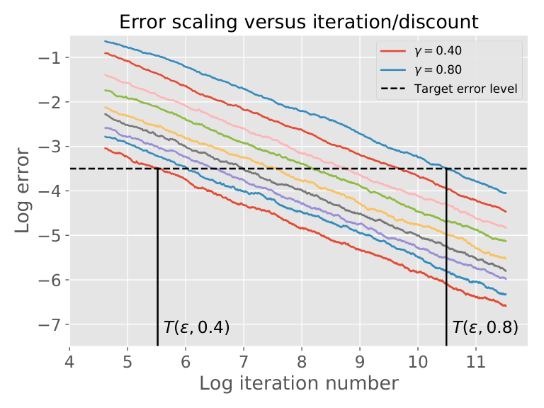
Consequently, by examining our iteration complexity bounds (26) and (28), we expect that for any fixed , the iteration complexity of -learning as a function of should be upper bounded as , and moreover, this bound should hold for either the rescaled linear stepsize, or the polynomial stepsize with . If our bounds cannot be improved in general, then we expect to see that this predicted bound is met with equality in simulation. Accordingly, our numerical simulations were addressed to testing the correctness of this prediction.
Figure 2 illustrates the results of our simulations. Panel (a) illustrates how the iteration complexity was estimated in simulation. For a given algorithm and setting of , we ran the algorithm for steps, thereby obtaining a path of -norm errors at each iteration . We averaged these paths over a total of independent trials. Given these Monte Carlo estimates of the average -error, for a given , we compute by finding the smallest iteration at which the estimated -error falls below . Panel (a) illustrates two instances of this calculation, for the settings and respectively.
For the fixed tolerance , we repeated this Monte Carlo estimation procedure in order to estimate the quantity for each , and then plotted the results on a log-log scale, as shown in panel (b). We fit each set of points with ordinary linear regression, yielding estimates of the slope and . We also applied a -test with the null hypothesis being that the slope is ; it returned -values of and in the polynomial and linear cases respectively. Thus, these simulations provide empirical evidence for the sharpness of our bounds in this ensemble of problems.
3.4.2 A non-sharp example
The example from the previous section shows that our bounds are unimprovable in general. However, there are instances for which our bounds are not sharp, with one the simplest being an MDP in which there is a root state that transitions (w.p. ) to one of two other states, both of which are absorbing. If we set the rewards at the two absorbing states to be and respectively, then the associated -functions at the two absorbing states will be and respectively. These highly discrepant values mean that the variance of the empirical Bellman operator at the root state will scale as . Consequently, our bounds yield guarantees with the rather pessimistic scaling , a behavior that is not observed in practice. The issue here is for problems of this type, the quantity is overly pessimistic, as it measures only the local variance (and not how fluctuations can be diminished by repeated applications of the Bellman operator). Resolving this gap requires a more sophisticated analysis, as in the work of Azar et al. [3] on model-based -fitting.
4 Discussion
The main contribution of this paper (Theorem 1) is a “sandwich” result for a class of stochastic approximation (SA) algorithms based on operators that satisfy monotonicity and quasi-contractivity conditions with respect to an underlying cone. This general result can be used to derive non-asymptotic error bounds for SA procedures with various stepsizes. We then illustrated this general result by applying it to derive non-asymptotic bounds for synchronous -learning applied to discrete state-action problems. We hope that this general result proves useful in analyses of other stochastic approximation algorithms.
This paper leaves open various questions. Our analysis covers both the cases of linearly decaying stepsizes, as well as the (more slowly decaying) polynomial choices for some . The advantage of polynomial stepsizes is that they are robust to the choices of constants; in contrast, the linear stepsize behaves badly unless it is suitably rescaled, requiring knowledge of the contraction coefficient. On the flipside, the polynomial choices perform more poorly in damping noise, so that the convergence guarantees show inferior scaling in the inverse tolerance . A standard resolution to this difficulty is to perform Polyak-Ruppert averaging [15, 16, 18]: that is, to run the algorithm with the slower polynomial stepsizes, and then average the iterates along the path with a stepsize. It would be interesting to extend our non-asymptotic analysis to the the class of SA procedures considered here combined with such averaging methods.
In the specific context of -learning, as we noted earlier, our results also show that standard -learning is a sub-optimal algorithm, in that we exhibited an example where its iteration complexity scales as , as opposed to the scaling that can be achieved by model-based batch -iteration [3]. Thus, our work highlights a gap between standard -learning as a model-free method and a model-based method, as has been done in recent work on the LQR problem [23]. It is natural to wonder whether this gap is specific to -learning, or also applies to other algorithms with essentially equivalent storage and/or computational requirements. We note that the speedy -learning algorithm [2], requiring only twice the storage of -learning, has been shown, in the setting considered here, to have worst-case iteration complexity scaling as .
Moving beyond the worst-case viewpoint, our bounds on -learning are instance-specific, depending on the unknown optimal -function via its variance (20) and span seminorm (21). These two quantities vary substantially over the space of MDPs with -bounded rewards, being much smaller than their worst-case values for many problems. Thus, it would be interesting to develop instance-based lower bounds on the performance of -learning and other algorithms. We note that such types of localized analysis have been given both in the bandit literature [9], and in non-parametric statistics [26].
Acknowledgements
Thanks to A. L. Z. Pananjady and K. B. B. Khamaru for helpful discussions. This work was partially supported by Office of Naval Research Grant ONR-N00014-18-1-2640 and National Science Foundation Grant NSF-DMS-1612948.
Appendix A Proof of Theorem 1
We begin by defining a recentered version of the updates (1). Subtracting from both sides yields the recentered recursion
Define the operator . With this notation, we see that the error sequence evolves according to the recursion
| (33) |
where we have re-introduced the effective noise variables , as previously defined in equation (5). By our assumptions on , we see that each one of the recentered operators is monotonic with respect to the cone , and contractive in the sense that for all .
We first prove the upper bound in equation (7) via induction on the iteration number . Beginning with the base case, for iteration , we have
where we have used the initialization conditions and .
We now assume that the claim holds at iteration , and show that it holds for iteration . We have
where the inequality follows from the inductive assumption; the monotonicity of the operator with respect to the cone; and the fact that . Now by the -contractivity of , we have
which establishes the claim in part (a).
Turning to the lower bound in part (a), again we proceed via induction on the iteration number . Beginning with the base case, for iteration , we have
as required.
We now assume that the claim holds at iteration , and show that it holds for iteration . We have
where the inequality follows from the inductive assumption, and the monotonicity of the operator on the cone. Now by the -contractivity of , we have
which completes the proof of the lower bound.
Appendix B Proofs for -learning
In this appendix, we collect the proofs of our results on -learning, beginning with the statements and proofs of some auxiliary lemmas in Section B.1 and followed by the proofs of Corollaries 3 and 4 in Sections B.2 and B.3 respectively.
B.1 Proofs of some auxiliary lemmas
In this appendix, we collect the statements and/or proofs of various auxiliary lemmas needed for the proofs of Corollaries 3 and 4.
B.1.1 Proof of Lemma 1
The inequality is a standard fact [17]; it follows by applying the triangle inequality to the definition of the span seminorm. Since is a fixed point of the Bellman equation (14), we have
from which it follows that as claimed.
Turning to the variance bound, from the definition of the empirical Bellman operator, we have
as claimed.
B.1.2 Controlling the MGF of non-stationary autoregressive processes
Let be a sequence of random variables and let be a sequence of stepsizes in . Define a new sequence of random variables via the non-stationary autoregression
| (34a) | ||||
| with initialization . Suppose that the stepsizes satisfy the inequality | ||||
| (34b) | ||||
The two choices of particular interest to us, both of which satisfy this inequality, are the rescaled linear stepsize , for which we have
and the polynomial stepsize , for which we have
where the inequality follows from the fact that .
Lemma 2 (Noise recursions).
Suppose that the noise sequence consists of i.i.d. variables, each with zero mean, bounded as almost surely, and with variance at most . Then for any sequence of stepsizes in the interval and satisfying the bound (34b), we have
| (35) |
Proof.
Given the assumed boundedness of , a standard argument (see Chapter 2 in the book [24]) yields that
| (36) |
We use this bound repeatedly in the argument.
We prove the claim (35) via induction on the index . The statement is vacuous for , since . We have . By the assumptions on , for any , we have
where step (i) uses the bound (36) with ; and step (ii) follows since .
We now assume that the claim holds at iteration , and then verify that it holds at iteration . We have
where equality (i) follows from the independence of and ; and inequality (ii) uses the bound (36) as well as the induction hypothesis, and holds for all . Once again using the assumed bound (34b) on the stepsizes, we have
This inequality is valid for any , which establishes the claim (35). ∎
B.1.3 Controlling the expected values of
We now state and prove a lemma that allows us to control the expected values of the -norms of the random sequence defined via the recursion (6a). The proof of this lemma makes use of Lemma 2.
Lemma 3 (Bounds on expected values).
Consider the sequence generated by some sequence of stepsizes in the interval and satisfying the bound (34b). Then there is a universal constant such that
| (37) |
Proof.
For a given , we have . Now each random variable is an autoregressive sequence of the type (34a), in which the underlying noise variables are bounded by , and have variance at most . Consequently, from the result of Lemma 2, we have
and hence
Since is a non-negative random variable, the result of Exercise 2.8 (a) in Wainwright [24] can be applied, and it yields the claimed bound (37). ∎
B.2 Proof of Corollary 3
Substituting the rescaled linear stepsize choice in the bound (9) from Corollary 1 and then taking expectations, we find that
| (38) |
Next we make use of the bound (37) from Lemma 3 to control the expected values in equation (38). Doing so yields
where and .
In order to complete the proof, it suffices to show that there is a universal constant such that
Beginning with the bound on and recalling our definition of the rescaled linear stepsizes, we have
Combining with the additional term yields the claimed bound on .
Turning to the bound on , we have
which establishes the claim.
B.3 Proof of Corollary 4
We now turn to the proof of our corollary on -learning with polynomial stepsizes . We require an auxiliary lemma on exponentially-weighted sums:
Lemma 4 (Bounds on exponential-weighted sums).
There is a universal constant such that for all and for all , we have
| (39a) | ||||
| (39b) | ||||
We return to prove this claim in Appendix B.3.1.
Taking Lemma 4 as given, we first take expectations over the noise in the bound (11) from Corollary 2. Using Lemma 3 to control the expected values yields
where
Applying Lemma 4 to bound and and performing some algebra completes the proof of Corollary 4.
B.3.1 Proof of Lemma 4
We prove the bound (39a). Define the function . By taking derivatives, we find that is decreasing on the interval and increasing for , where . Consequently, as long as , we have
Integrating by parts, we find that
where the final inequality uses the fact that is non-negative and decreasing on the interval . Substituting in the expression for , we find that
which implies that . Putting together the pieces, we have shown that
which establishes the claim of the first bound (39a). The proof of the second bound (39b) is analogous, so that we omit the details here.
Appendix C Details of the “hard” example
The only states with non-trivial variances are states and , for any action. For concreteness, let us focus on the state-action pair . We have
Note that for , and moreover , whence
which establishes the upper bound. As for the lower bound, we have
where we have used the fact that . As long as , then . In conjunction with the lower bound , we find that
which establishes the lower bound.
References
- [1] C. D. Aliprantis and R. Touky. Cones and duality, volume 84 of Graduate studies in mathematics. American Mathematical Society, 2007.
- [2] M. G. Azar, R. Munos, M. Ghavamzadeh, and H. J. Kappen. Speedy -learning. In Neural Information Processing Systems, pages 2411–2419, 2011.
- [3] M. G. Azar, R. Munos, and H. J. Kappen. Minimax PAC bounds on the sample complexity of reinforcement learning with a generative model. Machine Learning, 91:325–349, 2013.
- [4] F. Bach and E. Moulines. Non-asymptotic analysis of stochastic optimization algorithms for machine learning. In NIPS, December 2011.
- [5] A. Benveniste, M. Metivier, and P. Priouret. Adaptive Algorithms and Stochastic Approximations. Springer-Verlag, New York, NY, 1990.
- [6] D. P. Bertsekas. Dynamic programming and stochastic control, volume 1. Athena Scientific, Belmont, MA, 1995.
- [7] D. P. Bertsekas and J. N. Tsitsiklis. Neuro-Dynamic Programming. Athena Scientific, 1st edition, 1996.
- [8] V. S. Borkar. Stochastic Approximation: A Dynamical Systems Viewpoint. Cambridge, New York, NY, 2008.
- [9] S. Bubeck and N. Cesa-Bianchi. Regret analysis of stochastic and nonstochastic multiarmed bandits. In Foundation and Trends in Machine Learning, volume 5, pages 1–122. 2012.
- [10] E. Even-Dar and Y. Mansour. Learning rates for -learning. Journal of Machine Learning Research, 5:1–25, 2003.
- [11] T. Jaakkola, M. I. Jordan, and S. P. Singh. On the convergence of stochastic iterative dynamic programming algorithms. Neural Computation, 6(6), November 1994.
- [12] Z. Kadelburg, S. Radenovic, and V. Rakocevic. A note on the equivalence of some metric and cone metric fixed point results. Applied Mathematics Letters, 24:370–374, 2011.
- [13] H. J. Kushner and G. G. Yin. Stochastic Approximation Algorithms and Applications. Springer-Verlag, New York, NY, 1997.
- [14] A. Nemirovski, A. Juditsky, G. Lan, and A. Shapiro. Robust stochastic approximation approach to stochastic programming. SIAM Jour. Opt., 19(4):1574–1609, 2009.
- [15] A. S. Nemirovsky and D. B. Yudin. Problem Complexity and Method Efficiency in Optimization. John Wiley and Sons, New York, 1983.
- [16] B. T. Polyak and A. B. Juditsky. Acceleration of stochastic approximation by averaging. SIAM J. Control Opt., 30(4):838–855, 1992.
- [17] M. L. Puterman. Markov decision processes: Discrete stochastic dynamic programming. Wiley, 2005.
- [18] D. Ruppert. Efficient estimators from a slowly convergent Robbins-Monro process. Technical Report 781, Cornell University, 1988.
- [19] R. S. Sutton and A. G. Barto. Reinforcement Learning: An Introduction. MIT Press, Cambridge, MA, 2nd edition, 2018.
- [20] C. Szepesvári. The asymptotic convergence rate of -learning. In NIPS 10, pages 1064–1070, 1997.
- [21] C. Szepesvári. Algorithms for reinforcement learning. Morgan-Claypool, 2009.
- [22] J. N. Tsitsiklis. Asynchronous stochastic approximation and -learning. Machine Learning, 16:185–202, 1994.
- [23] S. Tu and B. Recht. The gap between model-based and model-free methods on the linear quadratic regulator: An asymptotic viewpoint. Technical report, UC Berkeley, February 2019.
- [24] M. J. Wainwright. High-dimensional statistics: A non-asymptotic viewpoint. Cambridge University Press, Cambridge, UK, 2019.
- [25] C. Watkins and P. Dayan. -learning. Machine Learning, 8:279–292, 1992.
- [26] Y. Wei, B. Fang, and M. J. Wainwright. From Gauss to Kolmogorov: Localized measures of complexity for ellipses. Technical report, UC Berkeley, March 2018. arxiv 1803.07763.