MmWave UAV Networks with Multi-cell Association: Performance Limit and OptimizationThanks: C.-H. Liu is with the Department of Electrical and Computer Engineering at Mississippi State University, Mississippi State, MS 39762, USA. K.-H. Ho and J.-Y. Wu are with the institute of Communications Engineering and Department of Electrical and Computer Engineering at National Chiao Tung University, Hsinchu 30010, Taiwan. The corresponding author is Dr. Liu (e-mail: chliu@ece.msstate.edu).

A channel in the network is generally considered as either a line-of-sight (LoS) or a non-line-of-sight (NLoS) one. If the channel is visually blocked from a user to a BS, it is NLoS and LoS otherwise. Since whether a channel is LoS or not highly depends on the network environment, we adopt the following low-altitude-platform (LAP) expression in [21] that generally characterizes the LoS probability of a channel between the typical user and UAV $U_{i}$ at height $H_{i}$ in different network environments [21]:

where $\|X_{u,i}\|$ denotes the Euclidean distance between the typical user and point $X_{u,i}$, $c_{1}$ and $c_{2}$ are environment-related constants (for rural, urban, etc.). All $H_{i}$’s for $i\in\mathbb{N}_{+}$ are assumed to be independent random variables (RVs). Note that (I-A) proposed in [21] is obtained by using a simple Sigmoid function to approximate the LoS probability of an air-to-ground channel from an LAP transmitter and it essentially indicates that only the elevation angle of a channel from a ground receiver to an LAP transmitter dominates the LoS probability of the channel. Also, note that $\rho(0)=1/(1+c_{2}\exp(c_{1}c_{2}))\triangleq\rho_{0}$ is not a function of $H_{i}$ and $\|X_{u,i}\|$ any more, i.e., whether the channel between the typical user and a UAV on the ground is LoS does not depend on the distance between them. To generally characterize the position of each UAV in the sky, we propose the following height distribution model of UAV $U_{i}$:

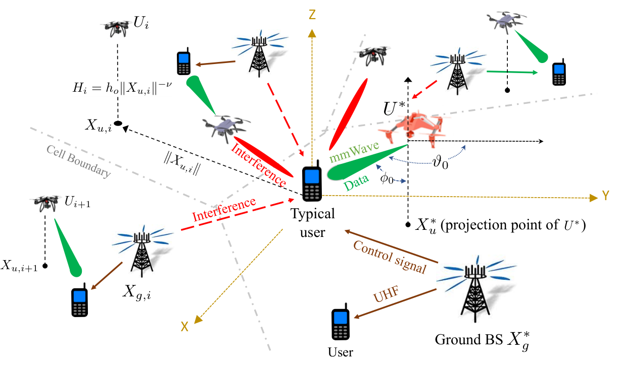
where $h_{o}\geq 0$ and $\nu\leq 0$ are constants. Namely, $H_{i}$ is a power-law function of the distance between the typical user and $X_{u,i}$ with parameters $h_{o}$ and $\nu$. Such a height model is motivated by the idea of suppressing the interference, that is, the horizontally farther interfering UAVs can hover either at a lower height to make their channels have a higher NLoS probability or at a higher height to make their channel undergo more path loss. Note that the proposed height distribution is so general that it can characterize many position control scenarios of the UAVs. For the case of $\nu=0$, for instance, all the UAVs are controlled to hover at the same height of $h_{o}$. For the case of $\nu=-1$, all the UAVs are controlled to maintain the same elevation angle of $\tan^{-1}(h_{o})$ from the typical user to them. Also note that the heights of the ground BSs are ignored in this paper since they are assumed to be fairly small compared with the heights of the UAVs. An illustration of the proposed mmWave UAV network with a plane-split architecture is depicted in Fig. 1.

Let $\mathds{1}(\mathcal{A})$ be the indicator function that is unity if event $\mathcal{A}$ is true and zero otherwise. The path-loss model between any BS $X_{i}\in\{X_{u,i},X_{g,i}\}$ and the typical user can then be written as

where $\alpha\triangleq\alpha_{g}\mathds{1}(X_{i}=X_{g,i})+\alpha_{u}\mathds{1}(X_{i}=X_{u,i})$ is referred to as the path-loss exponent; $\Psi_{i}\triangleq\Psi_{g,i}\mathds{1}(X_{i}=X_{g,i})+\Psi_{u,i}\mathds{1}(X_{i}=X_{u,i})$ and $\Psi_{u,i}$ ($\Psi_{g,i}$) is equal to $\psi_{u,L}$ ($\psi_{g,L}$) if the channel between $X_{i}$ and the typical user is LoS and equal to $\psi_{u,N}$ ($\psi_{g,N}$) otherwise. The physical meaning of $\psi_{u,L}$ ($\psi_{g,L}$) can be interpreted as the intercept of the LoS mmWave (UHF) channels, whereas the physical meaning of $\psi_{u,N}$ ($\psi_{g,N}$) can be interpreted as the integrated intercept and penetration loss of the NLoS mmWave (UHF) channels [2].

In the light of the plane-split architecture of the cellular network, each user should be associated with a ground BS and a UAV at the same time by adopting the following multi-cell association scheme:

where $X^{*}_{g}$ and $U^{*}$ denote the ground BS and the UAV associating with the typical user, respectively. Namely, each user is associated with the ground BS and the UAV that provide them with the minimum path loss. The path-loss distributions related to $U^{*}$ and $X^{*}_{g}$ are given in the following lemma.

In the previous subsection, the path-loss model between a BS and a user is specified, yet we would like to specify how to model the small-scale multiple-input-single-output (MISO) fading channel gain from a BS to a user in this subsection. For the tractability of analysis, we assume that all the users are equipped with a single antenna, while all the ground BSs and UAVs are equipped with $N_{g}$ and $N_{u}$ antennas, respectively³³ 3 To make the analyses much tractable in this paper, users are only considered to be equipped with a single antenna so that all analyses in the downlink are performed based on the MISO channel model, whereas all analyses in the uplink are proceeded based on the SIMO channel model. Nevertheless, all the analytical results are scalable to their corresponding counterparts with MIMO channels by using proper scaling techniques.. Hence, each downlink channel is a MISO channel and the fading channel gain of a channel from BS $X_{i}$ to the typical user can be modeled by

where $G^{*}_{g}\sim\text{Gamma}(N_{g},N_{g})$ denotes the beamforming fading channel gain⁴⁴ 4 Please note that the penetration loss of the NLoS channels of the ground BSs is already modeled in their path-loss model so that their fading gain does not need to consider the LoS effect. from $X^{*}_{g}$ and it is a Gamma RV with shape and rate parameters $N_{g}$, $G^{*}_{u}\sim\text{Gamma}(N_{u},N_{u})$ is the beamforming fading channel gain⁵⁵ 5 Here we implicitly assume that all the UAVs have a uniform rectangular array and they are able to perfectly steer their antenna array in all directions so as to maximize their antenna array gain from them to their serving users. from $U^{*}$, $G_{g,i}\sim\exp(1)$ is the fading gain from $X_{g,i}$ which is an exponential RV with unit mean, $G_{u,i}=\tilde{G}_{u,i}[\delta_{m}\mathds{1}(|\vartheta_{i}|\leq\vartheta_{0}\text{ AND }|\phi|\leq\phi_{0})+\delta_{s}\mathds{1}(|\vartheta_{i}|>\vartheta_{0}\text{ AND }|\phi_{i}|\geq\phi_{0})]$ denotes the transmit antenna array gain of $U_{i}$ in which $\vartheta_{0}$ and $\phi_{0}$ are the azimuth and the inclination of the main lobe, respectively; $\vartheta_{i}$ and $\phi_{i}$ are the boresight azimuth and the inclination of $U_{i}$, respectively (see Fig. 1); $\tilde{G}_{u,i}\sim\exp(1)$, $\delta_{m}$ and $\delta_{s}$ are the main lobe gain and side lobe gain of the antenna array of UAVs, respectively. Note that $\mathbb{P}[G_{u,i}=\delta_{m}\tilde{G}_{u,i}]=\frac{\vartheta_{0}}{2\pi}\times\frac{\phi_{0}}{\pi}$ and $\mathbb{P}[G_{u,i}=\delta_{s}\tilde{G}_{u,i}]=1-\frac{\vartheta_{0}}{2\pi}\times\frac{\phi_{0}}{\pi}$ since we assume $\vartheta_{i}$ is uniformly distributed over $[-\pi,\pi]$ and $\phi_{i}$ is uniformly distributed over $[-\pi/2,\pi/2]$. In the following subsection, we will apply the previously proposed path-loss model and the small-scale fading channel model to model two incomplete shot signal processes generated by the UAVs and ground BSs and investigate their statistical properties.

Without loss of generality, we assume that $U_{i}\in\Phi_{u}$ is the UAV that provides the typical user with the $i$th smallest path-loss among all the UAVs in $\Phi_{u}$. For the typical user, its 3D $K$th-incomplete shot signal process generated by the UAVs in the network is defined as

where $P_{u}$ denotes the transmit power of a UAV. Note that $I_{u,K}$ does not contain the signal powers generated by the $K$ UAVs in $\Phi_{u}$ that generate the first $K$ smallest path-loss signals received by the typical user so that it is called the $K$th-incomplete shot signal process. Similarly, the path loss from $X_{g,i}$ to the typical user is assumed to be the $i$th smallest one among all the path losses from all the ground BSs in $\Phi_{g}$. We then define the 2D $K$th-incomplete shot signal process of the typical user as follows:

where $P_{g}$ is the transmit power of the ground BSs and $\stackrel{{\scriptstyle d}}{{=}}$ stands for the equivalence in distribution. Likewise, $I_{g,K}$ does not include the first $K$ smallest path-loss signals among all path-loss signals generated by all the ground BSs. Note that we do not consider the void cell phenomenon⁶⁶ 6 In our previous works in [25, 23], we showed that user-centric cell association does not necessarily make each BS associate with at least one user. In other words, there could exist some void BSs whose cells do not have any users, which is called the void cell phenomenon. Since only non-void BSs generate interference and the number of the non-void BSs increases as the user intensity increases, we do not need to consider the void cell phenomenon in the interference model in (14) and (I-C) when the user intensity is assumed to be much larger than the BS intensity. in (14) and (I-C) because the user intensity is assumed to be so large that all the UAVs in the network associate with at least one user with high probability [25, 23].

Studying the statistical properties of $I_{u,K}$ and $I_{g,K}$ is crucial because it helps us understand how the aggregated signal powers from the UAVs and the ground BSs are affected by the network parameters (such as LoS/NLoS channel modeling parameters, BS intensities, etc.). In particular, we are interested in the Laplace transforms of $I_{u,K}$ and $I_{u,K}$ in that they will facilitate our following analyses. The Laplace transform of a non-negative RV $Z$ is defined as $\mathcal{L}_{Z}(s)\triangleq\mathbb{E}[\exp(-sZ)]$ for $s>0$, and thereby the Laplace transforms of $I_{u,K}$ and $I_{g,K}$ are found as shown in the following proposition.

According to the path-loss model in (5), the multi-cell association scheme in (I-A), the fading channel gain model in (I-B), and the $K$th-incomplete shot signal process in (14), the SINR of the typical user associating with UAV $U^{*}$ is defined as

where $\sigma^{2}_{u}$ is the noise power in the mmWave band and $I_{u,1}$ that is the 3D 1st-incomplete shot signal process based on (14) denotes the interference from all the interfering UAVs. Similarly, the SINR of the typical user associating with ground BS $X^{*}_{g}$ can be defined as

where $I_{g,1}$ is the 2D 1st-incomplete shot signal process accounting for the interference from all the interfering ground BSs. Note that there is no noise power term in (24) because the network in the UHF band is usually interference-limited. Using the SINRs defined in (23) and (24), we can define the multi-cell coverage (probability) of a user as follows⁷⁷ 7 The way of defining the multi-cell coverage in (25) is based on the consideration from the plane-split architecture of the UAV network, which is different from the way of defining the traditional signle-cell coverage. As we will see later on, the plane-split architecture also affects the definition of the channel rate of a user in (38). Note that actually other aspects of the UAV network are also impacted by the plane-split architecture, such as handover mechanism and resource allocation, and they are not addressed in this paper due to limited space.:

in which $\beta>0$ is the SINR threshold for successful decoding. The probability $\mathbb{P}[\gamma_{u}\geq\beta]\triangleq p_{u}$ is called the UAV coverage, whereas the probability $\mathbb{P}[\gamma_{g}\geq\beta]\triangleq p_{g}$ is called the ground coverage. The equality in (25) holds due to the independence between $\gamma_{u}$ and $\gamma_{g}$. This multi-cell coverage reflects how likely a user is able to successfully receive signals from its UAV and ground BS at the same time. Such a multi-cell coverage definition stems from the fact that the UAVs can successfully deliver their data to the users in the network only when the users can be simultaneously “covered” by their UAV and ground BS.

The multi-cell coverage of a user is derived as shown in the following proposition.

In this subsection, our focus is on how to maximize the multi-cell coverage by optimally deploying the ground BSs and UAVs as well as controlling the hovering positions of the UAVs. According to Proposition 2, we are able to see how the height distribution models of the UAVs with different values of $h_{o}$ and $\nu$ in (4) impact the coverage performance of the UAVs. Here we are particularly interested in two height control models of the UAVs, i.e., (constant) height control model and (constant) elevation angle control model. They are elaborated as follows.

Recall that the ground BSs and UAVs are in charge of the control and data planes of the network, respectively. Thus, whether the UAVs are able to effectively deliver data to the users highly depends on whether the users are able to successfully receive the control signals sent by the ground BSs. As a result of this plane-split architecture, the throughput of this mmWave UAV network needs to consider the ground coverage impact. The channel rate from UAV $U^{*}$ to the typical user can be characterized by the SINR in (23) and it is defined as

which indicates that $C_{u}$ is non-zero if and only if the users are covered by the ground BSs. It can be used to define the volume spectral efficiency (nats/sec/Hz/m³) of the mmWave UAV network as follows:

where $h_{\max}$ is the maximum height to which each UAV is able to fly up. Obviously, $V_{u}$ has the physical meaning of the throughput per unit bandwidth and volume of the network with the maximum height $h_{max}$ of a UAV if we interpret $\lambda_{u}/h_{\max}$ as the number of the UAVs in a unit volume of the network (i.e., the 3D intensity of the UAVs). The volume spectral efficiency in (III-A) can be alternatively expressed as

so that $V_{u}$ is apparently influenced by $p_{q}$ and $p_{u}$ since $\mathbb{P}[\gamma_{u}\geq x]$ is exactly equal to $p_{u}$ with $\beta=x$. Since $p_{g}$ depends on neither the intensity of the ground BSs nor the intensity of the UAVs, the only approach to efficiently increasing $V_{u}$ is to significantly improve $\lambda_{u}p_{g}p_{u}$. This will be explained in more detail later by using the explicit result of $V_{u}$ shown in the following Proposition.

References

- [1] S. Rangan, T. S. Rappaport, and E. Erkip, “Millimeter-wave cellular wireless networks: Potentials and challenges,” Proc. of The IEEE, vol. 102, no. 3, pp. 366–385, Mar. 2014.
- [2] T. S. Rappaport, J. George R. MacCartney, M. K. Samimi, and S. Sun, “Wideband millimeter-wave propagation measurements and channel models for future wireless communication system design,” IEEE Trans. Commun., vol. 63, no. 9, pp. 3029–3056, Sep. 2015.
- [3] X. Wang, L. Kong et al., “Millimeter wave communication: A comprehensive survey,” IEEE Commun. Surveys Tuts., vol. 20, no. 3, pp. 1616–1653, 3rd Quart. 2018.
- [4] Z. Xiao, P. Xia, and X.-G. Xia, “Enabling UAV cellular with millimeter-wave communication: Potentials and approaches,” IEEE Commun. Mag., vol. 54, no. 5, pp. 66–73, May 2016.
- [5] A. Fotouhi, H. Qiang et al., “Survey on UAV cellular communications: Practical aspects, standardization advancements, regulation, and security challenges,” IEEE Commun. Surveys Tuts., pp. 1–26, Early Access 2019.
- [6] Y. Zeng, R. Zhang, and T. J. Lim, “Wireless communications with unmanned aerial vehicles: Opportunities and challenges,” IEEE Commun. Mag., vol. 54, no. 5, pp. 36–42, May 2016.
- [7] M. Mozaffari, W. Saad, M. Bennis, and M. Debbah, “Efficient deployment of multiple unmanned aerial vehicles for optimal wireless coverage,” IEEE Commun. Lett., vol. 20, no. 8, pp. 1647–1649, Aug. 2016.
- [8] M. Alzenad, A. El-Keyi, F. Lagum, and H. Yanikomeroglu, “3-D placement of an unmanned aerial vehicle base station (UAV-BS) for energy-efficient maximal coverage,” IEEE Wireless Commun. Lett., vol. 6, no. 4, pp. 434–437, Aug. 2017.
- [9] V. V. Chetlur and H. S. Dhillon, “Downlink coverage analysis for a finite 3-D wireless network of unmanned aerial vehicles,” IEEE Trans. Commun., vol. 65, no. 10, pp. 4543–4558, Oct. 2017.
- [10] H. Wu, X. Tao et al., “Cooperative UAV cluster-assisted terrestrial cellular networks for ubiquitous coverage,” IEEE J. Sel. Areas Commun., vol. 36, no. 9, pp. 2045–2058, Sep. 2018.
- [11] X. Zhang and L. Duan, “Fast deployment of UAV networks for optimal wireless coverage,” IEEE Trans. Mobile Comput., vol. 18, no. 3, pp. 588–601, Mar. 2019.
- [12] A. V. Savkin and H. Huang, “Deployment of unmanned aerial vehicle base stations for optimal quality of coverage,” IEEE Wireless Commun. Lett., vol. 8, no. 1, pp. 321–324, Feb. 2019.
- [13] P. K. Sharma and D. I. Kim, “Random 3D mobile UAV networks: Mobility modeling and coverage probability,” IEEE Trans. Wireless Commun., vol. 18, no. 5, pp. 2527–2538, May 2019.
- [14] M. M. Azari, F. Rosas, and S. Pollin, “Cellular connectivity for UAVs: Network modeling, performance analysis and design guidelines,” IEEE Trans. Wireless Commun., pp. 1–15, Early Access 2019.
- [15] A. Chakraborty, E. Chai, K. Sundaresan et al., “SkyRAN: A self-organizing LTE RAN in the sky,” in Proc. ACM Int. Conf. on Emerging Netw. EXper. and Tech. (CoNEXT ’18), Dec. 2018, pp. 280–292.
- [16] M. Mozaffari, W. Saad, M. Bennis, and M. Debbah, “Wireless communication using unmanned aerial vehicles (UAVs): Optimal transport theory for hover time optimization,” IEEE Trans. Wireless Commun., vol. 16, no. 12, pp. 8052–8066, Dec. 2017.
- [17] Y. Zhu, G. Zheng, and M. Fitch, “Secrecy rate analysis of UAV-enabled mmwave networks using matérn hardcore point processes,” IEEE J. Sel. Areas Commun., vol. 36, no. 7, pp. 1397–1409, Jul. 2018.
- [18] L. Wei, R. Q. Hu, Y. Qian, and G. Wu, “Key elements to enable milliimeter wave communications for 5G wireless systems,” IEEE Wireless Commun., vol. 21, no. 6, pp. 136–143, Dec. 2014.
- [19] S. N. Chiu, D. Stoyan, W. S. Kendall, and J. Mecke, Stochastic Geometry and Its Applications, 3rd ed. New York: John Wiley and Sons, Inc., 2013.
- [20] M. Haenggi, Stochastic Geometry for Wireless Networks, 1st ed. Cambridge University Press, 2012.
- [21] A. Al-Hourani, S. Kandeepan, and S. Lardner, “Optimal LAP altitude for maximum coverage,” IEEE Wireless Commun. Lett., vol. 3, no. 6, pp. 569–572, Dec. 2014.
- [22] F. Baccelli and B. Błaszczyszyn, “Stochastic geometry and wireless networks: Volume I Theory,” Foundations and Trends in Networking, vol. 3, no. 3-4, pp. 249–449, 2010.
- [23] C.-H. Liu and L.-C. Wang, “Optimal cell load and throughput in green small cell networks with generalized cell association,” IEEE J. Sel. Areas Commun., vol. 34, no. 5, pp. 1058–1072, May 2016.
- [24] C.-H. Liu, “Coverage-rate tradeoff analysis in mmwave heterogeneous cellular networks,” IEEE Trans. Commun., vol. 67, no. 2, pp. 1720–1736, Feb. 2019.
- [25] C.-H. Liu and L.-C. Wang, “Random cell association and void probability in poisson-distributed cellular networks,” in IEEE Int. Conf. on Commun. (ICC), Jun. 2015, pp. 2816–2821.
- [26] T. Bai and R. W. Heath, “Coverage and rate analysis for millimeter-wave cellular networks,” IEEE Trans. Wireless Commun., vol. 14, no. 2, pp. 1100–1114, Feb. 2015.
- [27] C.-H. Liu and H.-C. Tsai, “Traffic management for heterogeneous networks with opportunistic unlicensed spectrum sharing,” IEEE Trans. Wireless Commun., vol. 12, no. 9, pp. 5717–5731, Sep. 2017.
- [28] M. Akdeniz, Y. Liu, M. Samimi, S. Sun, S. Rangan, T. Rappaport, and E. Erkip, “Millimeter wave channel modeling and cellular capacity evaluation,” IEEE J. Sel. Areas Commun., vol. 32, no. 6, pp. 1164–1179, Jun. 2014.
- [29] R. Amorim, H. Nguyen, P. Mogensen, and Others, “Radio channel modeling for UAV communication over cellular networks,” IEEE Wireless Commun. Lett., vol. 6, no. 4, pp. 514–517, Aug. 2017.
- [30] D. P. Bertsekas, Nonlinear Programming, 3rd ed. Belmont, MA: Athena Scientific, 2016.