Modal Group-Velocity Mismatch Induced Intermodal Modulation Instability in Step-index Fiber

The fiber used in our experiment is a step-index non-zero dispersion shifted CLF which is widely been used in communication. The fiber exhibits effective mode area and numerical aperture (NA) of 72 $\mu m^{2}$ and 0.14, respectively at 1550 nm. Pumping below the cut-off wavelength of the fiber, turns it into a few-mode fiber. At 1064 nm pump wavelength, the supported spatial modes through the fiber are simulated using full-vectorial finite-element method (FEM) based commercial COMSOL software and shown in Fig. 1. Simulated results show that the fiber supports $LP_{01}$, $LP_{02}$ and $LP_{11}$ spatial modes at the pump wavelength which are confirmed experimentally and will be discussed later. To demonstrate IM-MI, we excite the pair of circularly symmetric spatial modes $LP_{01}$ and $LP_{02}$ with equal peak power. The dispersion profile of two modes is shown in Fig. 2 and it is observed that the pump at 1064 nm falls in the normal dispersion region for both the modes. The step-index refractive index profile provides distinct group-velocity for different modes as shown in Fig. 3. It is observed that the GVM between the two modes increase with the increase in wavelength.

The nonlinear propagation of the interacting modes with identical carrier frequency $\omega$ satisfies the following set of coupled nonlinear Schrodinger equations (NLSE),

	$\displaystyle\frac{\partial u_{p}}{\partial z}-\frac{\delta_{pq}}{2}\frac{\partial u_{p}}{\partial t}+\frac{i}{2}\beta_{2p}\frac{\partial^{2}u_{p}}{\partial t^{2}}=i\gamma(\textit{f}_{pp}|u_{p}|^{2}$		(1)
	$\displaystyle+2\textit{f}_{pq}|u_{q}|^{2})u_{p}+i\gamma\textit{f}_{pq}u_{q}^{2}u_{p}^{*}exp(2i\Delta\beta z)$

	$\displaystyle\frac{\partial u_{q}}{\partial z}+\frac{\delta_{pq}}{2}\frac{\partial u_{q}}{\partial t}+\frac{i}{2}\beta_{2q}\frac{\partial^{2}u_{q}}{\partial t^{2}}=i\gamma(\textit{f}_{qq}|u_{q}|^{2}$		(2)
	$\displaystyle+2\textit{f}_{pq}|u_{p}|^{2})u_{q}+i\gamma\textit{f}_{pq}u_{p}^{2}u_{q}^{*}exp(-2i\Delta\beta z)$

where $u_{j}(j=p,q)$ is the field envelopes of the interacting modes, z is the propagation distance and t is the time. Nonlinear Kerr coefficient, $\gamma$=$\frac{n_{2}\omega}{c}$, c is the velocity of light in vacuum. $\Delta\beta=\beta_{q}-\beta_{p}$, where $\beta_{j}$ is the propagation constant of the corresponding mode, $\beta_{nj}=\frac{\partial^{n}\beta_{j}}{\partial\omega^{n}}$ stands for the nth derivatives of the propagation constant, $\beta_{1j}$ is the inverse of the group velocity, $\beta_{2j}$ is the second order dispersion coefficient. $\delta_{pq}$ indicates the GVM of the participating modes and defined as, $\delta_{pq}=\beta_{1q}-\beta_{1p}$. The overlap function $\textit{f}_{pq}$ is defined as,

$\displaystyle f_{pq}=\dfrac{\int\int|F_{p}(\omega)|^{2}|F_{q}(\omega)|^{2}\,dx\,dy}{[\int\int|F_{p}(\omega)||F_{q}(\omega)|\,dx\,dy]^{2}}$

(3)

where, $F_{p}$ and $F_{q}$ are the transverse field distributions of the participating modes. The effective mode area of the two modes can be expressed by $1/f_{pp}$ and $1/f_{qq}$, respectively, where, $1/f_{pq}$ represents the overlap between two interacting modes. We would like to point out that the coherent coupling terms $i\gamma\textit{f}_{pq}u_{q}^{2}u_{p}^{*}exp(2i\Delta\beta z)$ and $i\gamma\textit{f}_{pq}u_{p}^{2}u_{q}^{*}exp(-2i\Delta\beta z)$, in the right hand side of Eqs. (1) and (2), depend essentially on the GVM between the spatial modes. For large GVM, these terms are essentially negligible. As, in our case, we use step-index fiber which leads to large GVM between the interacting modes, thus the coherent coupling term is neglected in the preceding calculations. Considering only the incoherent coupling terms, Eqs. (1) and (2) can be rewritten as,

	$\displaystyle\frac{\partial u_{p}}{\partial z}-\frac{\delta_{pq}}{2}\frac{\partial u_{p}}{\partial t}+\frac{i}{2}\beta_{2p}\frac{\partial^{2}u_{p}}{\partial t^{2}}=i\gamma(\textit{f}_{pp}|u_{p}|^{2}$		(4)
	$\displaystyle+2\textit{f}_{pq}|u_{q}|^{2})u_{p}$

	$\displaystyle\frac{\partial u_{q}}{\partial z}+\frac{\delta_{pq}}{2}\frac{\partial u_{q}}{\partial t}+\frac{i}{2}\beta_{2q}\frac{\partial^{2}u_{q}}{\partial t^{2}}=i\gamma(\textit{f}_{qq}|u_{q}|^{2}$		(5)
	$\displaystyle+2\textit{f}_{pq}|u_{p}|^{2})u_{q}$

To analyze the stability of the steady state solution of Eqs. (4) and (5), we introduce a small first-order amplitude and phase perturbation u and v, where,

$\displaystyle u_{p}=(\sqrt{P}+u)exp[i\gamma(\textit{f}_{pp}P+2\textit{f}_{pq}Q)z]$

(6)

$\displaystyle u_{q}=(\sqrt{Q}+v)exp[i\gamma(\textit{f}_{qq}Q+2\textit{f}_{pq}P)z]$

(7)

Now, we consider perturbation of modulational ansatz with wavenumber K and frequency $\Omega$, of the form,

$\displaystyle u(z,t)=u_{s}(z)exp[i(\Omega t-Kz)]+u_{a}(z)exp[i(-\Omega t+Kz)]$

(8)

$\displaystyle v(z,t)=v_{s}(z)exp[i(\Omega t-Kz)]+v_{a}(z)exp[i(-\Omega t+Kz)]$

(9)

where, $u_{s}$ and $u_{a}$ represents the amplitude of Stokes and anti-Stokes sidebands for the spatial mode p, respectively, whereas $v_{s}$ and $v_{a}$ corresponds to the spatial mode q. $\Omega$ is the angular offset frequency relative to the pump, $\Omega=\omega-\omega_{p}$, where $\omega_{p}$ is the angular frequency for the pump wavelength. After linearizing Eqs. (4) and (5) in u and v and then substituting Eqs. (8) and (9) in it, we arrive at the following eigenvalue equation,

$\displaystyle[Y]=K[Y]$

(10)

where the eigen vector is defined as,

$\displaystyle{}^{T}=[u_{a},u_{s}^{*},v_{a},v_{s}^{*}]$

(11)

[M] is the stability matrix of the system defined as,

from which we obtain the following dispersion relation,

$\displaystyle det([M]-K[I])=0$

(12)

The equation implies that, for MI process to occur, the wavenumber K of the perturbation must possesses a non-zero imaginary part and manifest itself by an exponential growth of the amplitude of the perturbation. The power gain G, which is a measure of efficiency of MI process, is defined as, $G(\Omega)=2|Im(K)|$, where K is the eigenvalue of the matrix [M] with highest imaginary part. Detailed analysis of the Eq. (12) describes the necessary condition for MI phenomena as, $\sqrt{\textit{f}_{pp}\textit{f}_{qq}}/2f_{pq}<1$ IM_MI_greadedindex_fiber, i.e., the cross-phase modulation (XPM) term will be greater than self-phase modulation term (SPM). Table 1 shows the calculated values of IM-MI parameters for different mode combinations and indicates that among three different mode combinations, the condition to achieve IM-MI process has been satisfied for the mode group combination $LP_{01}$ and $LP_{02}$ only. For the theoretical calculations of MI gain of our experimental fiber, we have used the following parameters which have been calculated for the mode combination $LP_{01}$ and $LP_{02}$ of the CLF fiber at pump wavelength 1064 nm: $\beta_{2p}=0.01618$ $ps^{2}$/m, $\beta_{2q}=0.01183$ $ps^{2}$/m, $f_{pp}(1/\mu m^{2})=0.0257$, $f_{qq}(1/\mu m^{2})=0.0085$, $f_{pq}(1/\mu m^{2})=0.017$ and $\delta_{pq}=0.75ps/m$. The manifestation of IM-MI phenomena with varying peak pump power (P=Q) for the mode combination $LP_{01}$ and $LP_{02}$ is shown in Fig. 4 where the gain spectra have been plotted as a function of frequency detuning $\Omega$/2$\pi$ with different peak power levels. It is observed that IM-MI region broadens with the increase in power. The optimum modulation frequency (OMF) which is defined as the frequency at which IM-MI gain attain its maximum value, also shift towards higher value with the increase in pump power which also support our experimental findings. Finally the gain plot for varying GVM is shown in Fig. 5, where the power is kept fixed for both the modes at 3.75 kW. It is observed that large GVM leads to higher value of the gain spectra and simultaneously the optimal modulation frequency move towards longer frequency shift. Fig. 6 shows the variation of OMF and peak gain as a function of GVM of the participating modes. Simulated results reveal that peak gain increases gradually up to GVM 1.5 ps/m and then it tends to stabilize with further increasing GVM.

The schematic of the experimental setup is shown in Fig. 7. The pump is an output from Q-switched microchip Nd:YAG laser generating central wavelength at 1064 nm with the pulse duration of 0.77 ns. The output power of the pulses are controlled by the combination of HWP and PBS. The pump is coupled into CL optical fiber using microscope objective (NA=0.4, 20X).

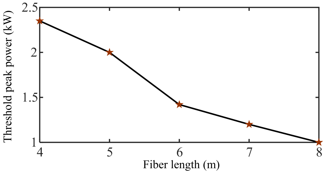
A three axis translational stage is used to excite selectively the desired modes and the output mode profile is detected with CCD as shown in the figure. The output spectrum is recorded by optical spectrum analyzer (OSA). All the supported spatial modes experimentally identified at 1064 nm are shown in Fig. 8 and agrees well with the simulated modal profiles as shown in Fig. 1. To study IM-MI, we have taken 6 m long CLF and pump is launched to excite the pair of modes ($LP_{01}$ and $LP_{02}$) with equal power in each modes. By finely adjusting the launching conditions of the pump pulses at the fiber input, we were able to excite equally the circularly symmetric modes. The recorded output spectrum with varying total input peak power is shown in Fig. 9. It is observed that with the increase in power, multiple MI sidebands are generated together with the Raman Stokes and anti-Stokes peaks. For 2.71 kW of peak power, IM-MI peaks are generated at wavelengths 1073 nm ($M_{1R}$) and 1056 nm ($M_{1L}$). Harmonics are generated in the red-side of the pump nearly at 1081 nm ($M_{2R}$) and 1090 nm ($M_{3R}$) whereas, on the blue-side of the pump at 1048.5 nm ($M_{2L}$) and 1040 nm ($M_{3L}$) wavelengths. Raman Stokes and anti-Stokes are generated at 1118 nm ($R_{1}$) and 1017.5 nm ($R_{2}$), respectively. The IM-MI gain for the pump power of 2.71 kW in each modes are shown in Fig. 10 which yields that maximum gain occurs at the frequency shift of $\pm\Delta$, where $\Delta=3.45$ THz. The position of the spectral peaks generated through 6 m fiber length with 2.71 kW pump power, are shown in Fig. 11 as a function of frequency shift from the pump wavelength. The IM-MI peaks are generated at $\Delta_{1}=-2.36$ THz and $\Delta_{2}=2.14$ THz apart. The asymmetry in frequency shift occurs due to the effect of higher order dispersion coefficient. Considering up to second-order dispersion coefficient, the position of the peaks of theoretical IM-MI gain are indicated by the dashed lines. The slight difference of the experimental and the theoretical observations are due to the refractive index profile that used in COMSOL for calculating dispersion parameters has been fitted and extrapolated at the pump wavelength (1064nm) from the original profile. To investigate the influence of fiber length, the evolution of IM-MI spectra for different fiber lengths with varying peak pump powers are measured and shown in Fig. 12. It is observed that, the threshold power require to build up spectral IM-MI peaks from noise gradually decreases with the increase in fiber length and shown in Fig. 13. Also, Raman threshold power reduces with the increase in fiber length. Longer fiber length provides effective platform to break-up the input pulses into multiple peaks through IM-MI even with sufficient low input pump power. Efficient IM-MI peaks with strong Stokes and anti-Stokes wave are generated with very low input pump power (2.43 kW in each mode) using 8m long CLF which is shown in Fig. 12 (d). The shift of spectral peaks with varying pump powers and fiber lengths is shown in Fig. 14(a) and 14(b), respectively. The fiber length has been fixed to 6 m. It is clearly evident that the IM-MI peaks and the cascaded harmonics exhibit shift in wavelength, as depicted in Fig. 14(a). The experimental observation of OMF shift of the IM-MI peaks as a function of peak pump power is shown by the solid line in Fig. 15, whereas the dashed line shows the theoretical prediction. The theoretical and the experimental lines shows almost same slope. It is important to note that MI peaks do not shift with the variation in fiber length, as shown in Fig. 14(b) where input peak pump power is fixed at 2.71 kW.

To conclude our work, we have reported detail theoretical and experimental observation of IM-MI in step-index scenario which yields that step-index multimode fiber can provide excellent platform for the realization of IM-MI. The modal GVM plays an important role in the gain spectrum and large GVM provides strong IM-MI peaks. Furthermore, details investigation with varying pump power and fiber length is demonstrated with unified manner. We also demonstrate the shifting of optimum frequency with pump power. The study can be effectively extended by employing large core step-index MMF which can support many higher order modes and launching the pump in different wavelength with non-identical spatial modes providing large GVM. The GVM can also be tailored by choosing the participating modes. Our observation will pave the way in multitude of applications such as the realization of coherent wideband frequency generation, formation of highly repetition rate vector soliton trains and so on.

References

- (1) C. Kharif and E. Pelinovsky, “Physical mechanisms of the rogue wave phenomenon”, Eur. J. Mech., vol. 22, no. 6, pp. 603-634, 2003.
- (2) M. Onorato, A. R. Osborne, M. Serio, and S. Bertone, “Freak waves in random oceanic sea states”, Physical Review Letters, vol. 86, no. 25, p. 5831, 2001.
- (3) H. Elbelrhiti, P. Claudin, and B. Andreotti, “Field evidence for surfacewave-induced instability of sand dunes”, Nature, vol. 437, no. 7059, p. 720, 2005.
- (4) K. E. Strecker, G. B. Partridge, A. G. Truscott, and R. G. Hulet, “Formation and propagation of matter-wave soliton trains”, Nature, vol. 417, no. 6885, p. 150, 2002.
- (5) V. Konotop and M. Salerno, “Modulational instability in Bose-Einstein condensates in optical lattices”, Physical Review A, vol. 65, no. 2, p. 021602, 2002.
- (6) A. Demircan and U. Bandelow,, “Supercontinuum generation by the modulation instability”, Optics communications, vol. 244, no. 1-6, pp. 181-185, 2005.
- (7) J. M. Dudley, G. Genty, F. Dias, B. Kibler, and N. Akhmediev, “Modulation instability, Akhmediev Breathers and continuous wave supercontinuum generation”, Optics express, vol. 17, no. 24, pp. 21497–21508, 2009.
- (8) S. Coen and M. Haelterman, “Continuous-wave ultrahigh-repetition-rate pulse-train generation through modulational instability in a passive fiber cavity”, Optics Letters, vol. 26, no. 1, pp. 39–41, 2001.
- (9) K. Tai, A. Hasegawa, and A. Tomita, “Observation of modulational instability in optical fibers”, Physical review letters, vol. 56, no. 2, p. 135, 1986.
- (10) M. Nakazawa, K. Suzuki, H. Kubota, and H. A. Haus, “The modulation instability laser. II. Theory”, IEEE journal of quantum electronics, vol. 25, no. 9, pp. 2045–2052, 1989.
- (11) E. Greer, D. Patrick, P. Wigley, and J. Taylor, “Picosecond pulse generation from a continuous-wave diode laser through cross-phase modulation in an optical fiber”, Optics letters, vol. 15, no. 15, pp. 851-853, 1990.
- (12) C. Menyuk, “Nonlinear pulse propagation in birefringent optical fibers”, IEEE Journal of Quantum electronics, vol. 23, no. 2, pp. 174-176, 1987.
- (13) S. Wabnitz, “Modulational polarization instability of light in a nonlinear birefringent dispersive medium”, Physical review A, vol. 38, no. 4, p. 2018, 1988.
- (14) J. E. Rothenberg, “Modulational instability for normal dispersion”, Physical review A, vol. 42, no. 1, p. 682, 1990.
- (15) T. Tanemura and K. Kikuchi, “Unified analysis of modulational instability induced by cross-phase modulation in optical fibers”, JOSA B, vol. 20, no. 12, pp. 2502-2514, 2003.
- (16) G. Millot, P. T. Dinda, E. Seve, and S. Wabnitz, “Modulational instability and stimulated Raman scattering in normally dispersive highly birefringent fibers”, Optical Fiber Technology, vol. 7, no. 3, pp. 170-205, 2001.
- (17) K. Nithyanandan, R. V. J. Raja, K. Porsezian, and B. Kalithasan, “Modulational instability with higher-order dispersion and walk-off in Kerr media with cross-phase modulation”, Physical Review A, vol. 86, no. 2, p. 023827, 2012.
- (18) R. Ganapathy, K. Senthilnathan, and K. Porsezian, “Modulational instability in a fibre and a fibre Bragg grating”, Journal of Optics B: Quantum and Semiclassical Optics, vol. 6, no. 5, p. S436, 2004.
- (19) G. Millot, S. Pitois, and P. T. Dinda, “Modulational instability processes in optical isotropic fibers under dual-frequency circular polarization pumping”, JOSA B, vol. 19, no. 3, pp. 454–460, 2002.
- (20) P. Drummond, T. Kennedy, J. Dudley, R. Leonhardt, and J. Harvey, “Cross-phase modulational instability in high-birefringence fibers”, Optics communications, vol. 78, no. 2, pp. 137-142, 1990.
- (21) E. Seve, P. T. Dinda, G. Millot, M. Remoissenet, J. Bilbault, and M. Haelterman, “Modulational instability and critical regime in a highly birefringent fiber”, Physical review A, vol. 54, no. 4, p. 3519, 1996.
- (22) M. Guasoni, “Generalized modulational instability in multimode fibers: Wideband multimode parametric amplification”, Physical review A, vol. 92, no. 3, p. 033849, 2015.
- (23) J. H. Li, H. Xu, T. T. Sun, S. X. Pei, and H. D. Ren, “Effects of intermode nonlinearity and intramode nonlinearity on modulation instability in randomly birefringent two-mode optical fibers”, Optics Communications, vol. 415, pp. 74–81, 2018.
- (24) R. Dupiol, A. Bendahmane, K. Krupa, J. Fatome, A. Tonello, M. Fabert, V. Couderc, S. Wabnitz, and G. Millot, “Intermodal modulational instability in graded-index multimode optical fibers”, Optics letters, vol. 42, no. 17, pp. 3419-3422, 2017.