An Energy-Efficient Controller for Wirelessly-Powered Communication Networks Part of this work has been accepted for presentation at ICC 2019.
Abstract
In a wirelessly-powered communication network (WPCN), an energy access point (E-AP) supplies the energy needs of the network nodes through radio frequency wave transmission, and the nodes store their received energy in their batteries for possible data transmission. In this paper, we propose an online control policy for energy transfer from the E-AP to the wireless nodes and for data transfer among the nodes. With our proposed control policy, all data queues of the nodes are stable, while the average energy consumption of the network is shown to be within a bounded gap of the minimum energy required for stabilizing the network. Our proposed policy is designed using a quadratic Lyapunov function to capture the limitations on the energy consumption of the nodes imposed by their battery levels. We show that under the proposed control policy, the backlog level in the data queues and the stored energy level in the batteries fluctuate in small intervals around some constant levels. Consequently, by imposing negligible average data drop rate, the data buffer size and the battery capacity of the nodes can be significantly reduced.
I Introduction
Smart electronic devices are increasingly making their way into our daily life. It is predicted that by 2021, there will be around 28 billion connected devices all over the world [1], a great number of which will be portable and battery-powered. However, in some applications such as biomedical implants inside human bodies [2] or distributed monitoring sensors, replacing the batteries may be infeasible. As such, the problem of providing the required energy for the portable battery-operated devices has recently received growing attention, both in academia and industry [3, 2]. Particularly, the idea of charging batteries over the air is considered as a promising solution which guarantees an uninterrupted connection and reduces the problem of massive battery disposal. The key enabling technology for charging over the air is wireless energy transfer (WET). There are various WET methods including electromagnetic radiation [3], resonant coupling [4] and inductive coupling [5]. Compared to the two latter methods, electromagnetic radiation provides a wider coverage range and is more flexible for transmitter/receiver deployment and movement [2].
There are numerous studies on energy beamforming as a technique for alleviating the high transmission path loss in wirelessly-powered communication networks (WPCNs) [6, 7, 8, 9] as well as for the simultaneous wireless information and power transfer systems [10, 11, 12]. Moreover, [13, 14, 15, 16, 17, 18, 19, 20] consider cooperation among the users as a useful method to increase the network coverage in two-hop [13, 14, 15, 16, 17, 18] and multi-hop [19, 20] WPCNs, respectively. Furthermore, [21] and [22] study the reliability of data transmission in WPCNs.
In the networks that support continuous or regular communication, the nodes are equipped with batteries which enable them to store their harvested energy in one time-slot for possible use in the subsequent time-slots [23, 24, 25, 26]. In such cases, the network performance should be analyzed in the long term, because a single time-slot analysis may not be optimal in general. For this reason, [23] and [24] study the long-term network throughput optimization through Markov decision processes (MDP). Moreover, in [25, 26, 27, 28, 29], long-term energy optimality and fairness for a multi-user downlink WET scenario are studied through Lyapunov optimization technique.
In this work, we design an energy-efficient WET policy that jointly controls data-link power allocation, data routing, energy beamforming and data/energy transmission time sharing in a multi-hop WPCN. The problem is cast in the form of minimizing the total average energy consumption of the network subject to stability of the data queues in the network and the battery level constraints of the nodes. The battery level constraint complicates finding the optimal control policy, since high energy consumption in one time-slot degrades the battery level of the node considerably, which may lead to energy outage in the subsequent time-slots. Therefore, the optimal decisions in different time-slots are coupled. This coupling makes finding the optimal policy challenging.
We use Lyapunov optimization method with a novel quadratic Lyapunov function to avoid energy outage. Based on the proposed Lyapunov function, we propose an online control policy called energy-efficient controller for WPCN (EECW), that does not require the explicit knowledge of the channel statistics. With the proposed policy, the time-slots are devoted to either energy transfer or data transmission. In energy transmission time-slots, the energy beam is focused towards the nodes with low battery levels, higher queue backlogs and higher energy-link channel gains. In data transmission time-slots, the data is routed through the nodes with less congested queues and higher battery levels.
We analyze the performance of the proposed control policy and prove that for every arbitrarily chosen value of a parameter in our algorithm, the energy consumption under EECW is within a bounded gap of the order of to the optimal policy, while the average backlog of data queues is upper bounded by . In addition, we show that the backlog level of the data queues and the energy level of the batteries converge probabilistically to some constant values, with the probability of deviation from those values decreasing exponentially with respect to the amount of deviation. Using this result, we further propose a modified version of EECW which can significantly reduce the required size of the data buffers in the nodes as well as the required capacity of their batteries, while imposing a negligible drop rate in the network. Finally, we present extensive simulations to provide insightful intuitions on the advantages of the proposed control policy, in terms of its energy requirements for stabilizing a WPCN.
As opposed to [6, 7, 8, 9, 10, 11, 12, 13, 14, 15, 16, 17, 18, 19, 20], we consider battery-powered nodes and analyze the network performance in the long term, instead of a single time-slot analysis. In contrast to [6, 7, 8, 10, 11, 12, 13, 14, 15, 16, 17, 18, 19, 20, 27, 28, 29, 24, 23, 21, 22], which analyze the throughput, the delay or the outage probability, we study the optimization of the energy consumption while the data queues are stabilized. Finally, different form [21, 22, 6, 7, 8, 9, 10, 11, 25, 26, 27, 28, 29, 24, 23], we study a general multi-hop WPCN where the data should be routed through the nodes. The differences in the system model and the problem formulation makes our results and analysis completely different from those in [6, 7, 8, 9, 10, 11, 12, 13, 14, 15, 16, 17, 18, 19, 20, 25, 26, 27, 28, 29, 24, 23, 21, 22].
The rest of the paper is organized as follows. The considered system model and our problem formulation are illustrated in Section II. The proposed control policy as well as its performance analysis is presented in Section III. The behavior of the data backlog in the queues and the energy level in the batteries are analyzed in Section IV. Some implementation issues are discussed in Section V. Simulation results are presented in Section VI, and finally, Section VII concludes the paper.
Notation: Matrices and vectors are denoted by small and capital boldface letters, respectively. Moreover, unless otherwise mentioned, vectors are single row-matrices. Also, , and denote transpose, conjugate transpose and element-wise conjugate of a matrix, respectively. Finally, denotes the absolute value (or the modulus for complex numbers), denotes the norm of vectors, represents the expectation and .
II System Model
| Symbol | Definition |
|---|---|
| Number of nodes, streams and data links, respectively. | |
| The backlog of data queue allocated to stream at node in time-slot . | |
| The battery level of node in time-slot . | |
| The head and tail node of link , respectively. | |
| The set of outgoing links from and incoming links to node , respectively. | |
| The energy stored in and drained from the battery of node in time-slot , respectively. | |
| The limitation on and (i.e., ) | |
| The beamforming vector and the transmission power of the E-AP in time-slot , respectively. | |
| The instantaneous data of stream arrived at node , in time-slot . | |
| The data arrival rate of stream at node . | |
| The total amount of data of stream that enters to and exits from node in time-slot , respectively. | |
| The limit on and (i.e., ) | |
| The vector of data link channel states in time-slot . | |
| The vector of energy link channel gains for node in time-slot . | |
| The vector of power allocations to data links in time-slot . | |
| The set of feasible data-link power allocation vectors. | |
| The rate-power function of link in time-slot . | |
| The instantaneous data rate of stream over link in time-slot . | |
| Maximum admissible transmission power of the wireless nodes and the E-AP, respectively. | |
| Time-slot duration and fraction of time-slot devoted to data and energy transmission, respectively. |
The notations used in the paper along with their definitions are presented in Table I. We consider a WPCN consisting of one energy access point (E-AP) and wireless nodes, with streams of data between distinct endpoints in the network. It should be noted that our analysis can be extended to consider multiple E-APs. However, for simplicity we focus on networks with a single E-AP. The wireless nodes are battery-powered, and the batteries are recharged by the energy received from the E-AP. The E-AP is equipped with antennas to focus its transmission beam towards the nodes. Moreover, we assume that the nodes use a single antenna for both energy reception and data transmission/reception. There exist energy links between the E-AP and the nodes and data links between the nodes. The topology of a sample network is depicted in Fig. 1(a). For each data link , and denote the head node and the tail node of link , respectively. Moreover, we define and as the sets of the incoming and outgoing data links of node , respectively.
The time horizon is divided into time-slots with fixed length, indexed by . Figure 2 shows the structure of a time-slot. At the beginning of each time-slot , a small interval is devoted to channel estimation and control signaling. The rest of the time-slot is divided into two intervals of lengths and , for energy and data transmission, respectively. We have where is the fixed portion of the time-slot allocated for data and energy transmission.
The channel coefficients are assumed to be constant during a time-slot but vary randomly and independently in successive time-slots. Recall that the E-AP has multiple antennas whereas the wireless nodes use a single antenna for both energy reception and data transmission/reception. In each time-slot , and represent the channel gains of the link between nodes and and the link between the -th antenna of the E-AP and node , respectively. Accordingly, we define and as the channel gain vectors for data links and energy link of node , respectively. Note that here the energy links are numbered according to the ID of the energy receiving node whereas the data links are independently numbered.
-
Data and Energy Transmission Let denote the data-link power vector, in which the -th entry is the allocated transmission power over the -th data link. Moreover, let denote the finite set of all feasible power vectors. We assume that setting an element of a power vector in to zero results in a new power vector that also belongs to . Furthermore, we assume that the maximum total transmit power of each node is limited to . Let denote the rate-power function in link under the allocated data-link power vector and the channel gain vector . Consider two feasible power vectors and , where and . We assume that the rate-power functions under each of these two power vectors satisfy the following properties
(1) (2) (3) As an example of , the reader may think of
(4) where is the set of the links that interfere with link . Equation (4) is an appropriate approximation for the achievable rates in the cases with codewords of moderate/large length. However, as we show in Section VI, our analysis is also applicable to the case of codewords of finite length, which results in a different rate-power function. Note that the properties (1), (2) and (3) are easily satisfied by conventional rate-power functions. Equation (1) indicates that no data can be passed through a data link if no power is assigned to that link. Inequality (2) is satisfied by functions with bounded first derivative. Finally, inequality (3) holds due to the interference effect among wireless links. Let denote the transmission rate allocated to stream in link . The sum rate of all streams in link should not exceed the achievable rate of that link. Therefore, a feasible rate allocation scheme should satisfy
The E-AP performs energy beamforming to concentrate its transmit energy towards the nodes. Let denote the normalized beamforming vector of the E-AP. Accordingly, the received energy at each node , denoted by , is given by
(5) where is the E-AP’s transmitted energy and is the E-AP’s transmit power in time-slot . The peak transmission power of the E-AP is limited to , i.e.,
-
Wireless Nodes As shown in Fig. 1(b), each node includes data queues and a battery. Let denote the level of the stored data for stream in node at the beginning of time-slot . Moreover, let and denote the number of data units of stream that enter to and exit from node during time-slot , respectively. Accordingly, evolves as
(6) The parameters and are determined through the assigned transmission rates and the external data arrivals, that is,
(7) and
(8) where is the number of external data units of stream that enter node in time-slot . We assume that is a random variable following an identical and independent distribution in different time-slots. We denote the mean value of by , and we have if node is the source of stream and otherwise. We denote the vector of arrival rates by . Furthermore, we assume that and are both upper bounded by .
The battery of each node is recharged by the energy received from the E-AP and is (partially) discharged when the node transmits data. Let denote the energy level stored in the battery of node at the beginning of time-slot . Therefore, the battery level at node evolves according to
(9) where is the total energy consumption of node in time-slot and is the portion of the received energy that is stored in the battery of node in time-slot . Intuitively, we expect that a node stores all its received energy from the E-AP, i.e., , but due to the wide transmission beam of the E-AP some nodes may receive more energy than they need. Specifically, in some network topologies, the nodes with low energy consumption may receive parts of the energy that is transmitted towards the nodes with higher energy consumption. Accordingly, the stored energy in the batteries of the low energy consumption nodes may grow unbounded. Thus, we let . That is, the nodes may store only a portion of their received energy. We further assume that and are both upper bounded by , and, consequently, we have and .
-
Network Controller There exists a network controller, located at the E-AP, that controls both the data and the energy links, having access to channel state information (CSI) and the level of the stored data and energy in the queues and batteries of all nodes11 1 We ignore the cost of the nodes sending feedback to the E-AP to inform it about the CSI and stored data/energy. . The network controller schedules data/energy transmission time sharing by specifying and . Moreover, it controls the energy links by specifying the E-AP transmission power and the beamforming vector and controls the data links by determining their power vector and data routing through specifying .
Let denote the minimum achievable average energy consumption per time-slot of the E-AP over all stabilizing polices. We define as a function of E^opt (λ)t
III The Proposed Control Policy
In this section, we construct the EECW. The general idea behind the EECW is to prevent the queue backlog from growing large, while the energy levels in the batteries of the nodes are kept at an appropriate level in proportion to their stored data backlog level. For this purpose, we introduce the imbalance indicators , as
| (11) |
where , for some . Note that represents an energy to data conversion factor. The value of indicates the data/energy imbalance at node in time-slot . For constructing the EECW, we follow the MDPP approach. In summary, we follow the following steps:
- 1.
We define the Lyapunov function as
(12) where and are the vectors of the backlog level in the data queues and the imbalance indicators, respectively. According to (12), the Lypunov function grows if the stored data level in the queues and/or the data/energy imbalance increases. As a result, we intuitively expect a stabilizing controller to prevent the Lyapunov function from growing large.
- 2.
We define the Lypunov drift function, which is the expected increment of the Lyapunov function in successive slots, i.e.,
(13) where the expectation is with respect to the randomness in the data and the energy channel gains and the data arrivals.
- 3.
We define the drift-plus-penalty function as
(14) where is a control parameter. We will derive an upper bound for in Lemma 1.
- 4.
- 5.
The details of the analysis are explained as follows. First, Lemma 1 derives an upper bound on .
Lemma 1.
Proof.
See Appendix A. ∎
The terms in (16) can be rearranged to better demonstrate as a function of the control variables. Particularly, we write
| (17) |
where
| (18) | ||||
and
| (19) | ||||
The equality in (17) can be verified by adding and subtracting to (16) and using the definitions for , , and . The EECW is designed to approximately minimize the right hand side of (15). In this way, the control policy under the EECW follows the following procedure:
Initialization: Set dummy data units in data queues, i.e., and assume .
Data Routing in time-slot : Calculate the weights according to (19). Let
| (20) |
and
| (21) |
The total capacity of link is assigned to stream , i.e.,
| (22) |
Data link scheduling in time-slot : The transmission power vector is determined by solving
| (23) |
Energy link scheduling in time-slot : The energy beamforming vector is determined as
| (24) |
where is the principal eigenvector of defined as
| (25) |
The transmission power of the E-AP is determined by
| (26) |
Data/Energy time sharing in time-slot : Let
| (27) |
and
| (28) |
where , and are determined in (23), (24) and (26), respectively. The time sharing rule is
| (29) |
Queues and batteries update in time-slot : The portion of the received energy that is stored in the battery is determined by
| (30) |
The data queues and batteries are then updated according to (6) and (9), respectively.
The EECW policy for controlling the data link and the energy link are summarized in Algorithms 1 and 2, respectively.
III-A Discussion on the Proposed Control Policy
Considering (19), the value of increases if the data queue in node is less congested and/or if there is less data/energy imbalance in node . Hence, according to the routing policy in (22), we expect that with EECW the data will flow towards the nodes with less congested queues and less data/energy imbalance. The power allocation policy in (23) devises a compromise between the energy consumption penalty represented by , and the data transmission reward represented by . The beamforming policy implies that the energy beam is focused towards the nodes with higher data/energy imbalance and higher energy-link channel gains. Moreover, considering the E-AP transmission power scheduling in (26), the control parameter can be described as the energy conservativeness indicator of the EECW, since by increasing the E-AP transmits less often.
The time sharing control parameters, and , can be described as two metrics representing the gain for data and energy transmission in time-slot , respectively. These two parameters take into account the level of the stored energy and data in the nodes as well as the CSI to determine the energy/data transmission gain. Finally, the policy for storing the received energy in (30) implies that with a small value of a portion of the received energy may not be stored in the battery, which prevents the battery from being overcharged. Note that this event mostly occurs when the energy-link channels are not orthogonal, i.e., . Otherwise, according to (25) and for a small value of , the beamforming vector will be almost orthogonal to . Hence, the received energy in node will be negligible.
III-B Performance Analysis of the Proposed Control Policy
In this section, we evaluate the performance of the proposed policy. In this regard, Lemma 2 introduces some properties that are satisfied with EECW in each time-slot. Particularly, we show in Lemma 2 that the battery constraint (II) is satisfied. In Lemma 3, we use the properties of Lemma 2 to show that EECW approximately minimizes the right hand side of (15). Finally, we use the result in Lemma 3 to evaluate the energy consumption with EECW and to show that the backlog in the queues satisfy (II). First, we present Lemma 2.
Lemma 2.
With the EECW, in each time-slot , we have that
- 1.
The imbalance indicator , satisfies .
- 2.
The assigned rate is nonzero only if .
- 3.
The drained energy is nonzero only if .
Proof.
See Appendix B. ∎
The first part of Lemma 2 ensures that the stored amounts of energy in the batteries are bounded in proportion to the stored backlog in the data queues of the nodes, i.e., . The second part in Lemma 2 implies that there will be enough data for transmission, when the outgoing rate from a node is nonzero. Hence, with EECW, we have . Moreover, the third part in Lemma 2 guarantees that when a node transmits data, i.e., , we have . Hence, EECW conforms to the battery constraint (II).
Using the properties in Lemma 2, it can be shown that the EECW approximately minimizes the right hand side in (15). Specifically, with , it suffices to show that EECW approximately minimizes in (16). For this reason, let denote the minimum value of in time-slot over every alternative policy, including the policies that violate the battery constraint (II), i.e.,
| (31) | ||||||
Lemma 3 presents the gap between under EECW and .
Using the bound in (32), and following the Lyapunov optimization Theorem [30, Theorem 4.2], we compare the energy consumption under EECW with and bound the time-averaged expected backlog in the queues. Specifically, let denote the set of data arrival rates that are inside the capacity region of the network. Hence, Problem () is feasible if and only if . Theorem 1 characterizes the performance of the EECW when is strictly inside . Particularly, parts 1 and 2 of Theorem 1 show the optimality of the energy consumption and the stability of the network under EECW, respectively.
Theorem 1.
Suppose that the arrival rates are strictly inside the capacity region, i.e., there is a scalar such that , where is a vector with all entries equal to . With our proposed EECW,
- 1.
The time-averaged expected energy consumption satisfies
(33) - 2.
The queues are stable and the time-averaged expected sum backlog satisfies
(34)
where .
Proof.
See Appendix D. ∎
The performance bounds in (33) and (34) introduce a trade-off between the optimality gap and the average queue backlog that is controlled by . According to this trade-off, when the average energy consumption is within of the minimum energy, the average backlog could be upper bounded by a term of the order of .
IV Time Evolution of Data Backlog and Battery Level
Theorem 1 bounds the average backlog in the queues. However, it does not discuss the behavior of the backlogs and the battery levels, which are of importance for the implementation of the policy. In this section, we study the time evolution of the data backlog and the battery level under EECW using the backlog attraction result in [31]. We show that with EECW the data backlog and the battery level converge to a transformation of the dual optimal solution for the following deterministic problem
| (35a) | ||||||||
| (35b) | ||||||||
| (35c) | ||||||||
| (35d) | ||||||||
The solution to (35) is a stationary policy that is only a function of the instantaneous CSI. Hence, we have omitted the time averages. Specifically, let with denote the dual function of Problem (35), that is,
| (36) |
and let denote the optimal solution to the dual problem, i.e.,
| (37) |
Let be constructed from as
| (38) | ||||
| (39) |
Moreover, let be constructed from as
| (40) |
Theorem 2 presents the main result on the behavior of queue backlogs and battery levels.
Theorem 2.
Suppose that the dual function (36) satisfies
| (41) |
for some . Then, with the EECW, there exists constants , and independent of such that for every we have
| (42) | ||||
| (43) |
Proof.
See Appendix E. ∎
Theorem 2 shows that the probability that the backlog in data queues and energy level in batteries deviate from and , respectively, decreases exponentially as the deviation increases. Note that the assumption in (41) holds when the control parameters are chosen from a finite set [31] which is the case for the digital implementation of the algorithm.
V EECW Implementation
In this section, we discuss some implementation issues related to EECW. Specifically, we study the effect of the limited-capacity data buffers and batteries and the complexity of our proposed policy.
V-A Limited Data Buffers and Batteries
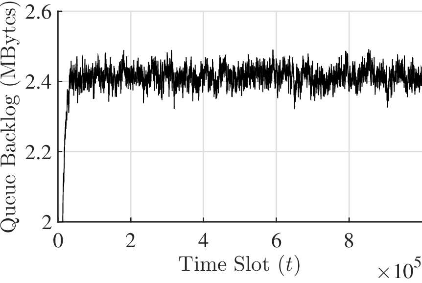
A challenge for the implementation of EECW is the limited buffer size and battery capacity of the nodes. Theorem 2 ensures that with sufficiently large batteries and buffers the probability of data or energy overflow is small. Hence this limitation does not affect the performance of the policy. Figure 3 depicts a sample time evolution of the backlog and battery level under EECW. As can be seen, the backlog converges to a constant value. Also, with a buffer size of and a battery capacity of there will be no overflow. However, the behavior of the backlog suggests that, if we tolerate dropping a small amount of data in the initialization phase of the algorithm, we can further reduce the buffer size and battery capacity. Specifically, in the steady state region of Figs. 3(a) and 3(b) the backlog and the battery level fluctuate approximately in and intervals, respectively, which implies that the arrival and departure processes in steady state can be supported by a buffer and a battery. This observation motivates us to modify EECW for limited buffer size and battery capacity implementation. For this reason, we define virtual queues and associated with each real and finite data queue and battery, respectively. The virtual queues are not physical queues and are simple counters inside the controller that are updated as
| (44) | ||||
| (45) |
EECW runs based on the values of and instead of the real queues, hence , , and will have exactly the same value as we had in the cases with infinite length real data queue and batteries. Accordingly, the limited buffer sizes and battery capacities do not affect the decisions of the controller. However, some data units in real buffers may be dropped due to either buffer overflow or energy outage. Let denote the total number of dropped data units of stream in node up to time-slot . Lemma 4 bounds the time averaged expected value of under the modified EECW for limited buffers and batteries.

Lemma 4.
Let and denote the size of the data buffers and the capacity of the batteries, respectively. Suppose that and . With the modified EECW, we have
| (46) |
where
| (47) |
Proof.
See Appendix F. ∎
Lemma 4 states that the average drop rate decreases exponentially as the buffer size or the battery capacity increases.
V-B Complexity of the Proposed Policy
The most computationally expensive part of EECW is solving Problem (23), which is similar to the well known max-weight problem. Under the common interference models, this problem is nonconvex and can be NP-hard [32]. However, many efficient approximate and distributed solutions are proposed for the max-weight problem [33, 34, 35], that can be extended to solve (23). As an example, [33] introduces a distributed iterative algorithm based on the block coordinate descent method for solving a problem similar to (23).
Note that using the same arguments as in [36], it can be shown that a suboptimal scheduling in each time-slot may result in satisfactory overall performance. Specifically, instead of (32), if the suboptimal scheduler satisfies
| (48) |
in each time-slot and for some and , the time-averaged expected energy consumption per time-slot will be close to . Accordingly, we may use approximate schedulers with low complexity or reduce the overhead for CSI estimation, while remains close to unity and the performance loss is negligible. Below, we study the performance loss due to imperfect CSI through simulation.
VI Simulation Results
In this section, we consider a wireless network consisting of one E-AP and nine wireless nodes, as shown in Fig. 4(a). In this network, there are two streams of data, from nodes 1 and 2 to nodes 6 and 9, respectively. We consider the node exclusive model in which the data links are orthogonal but each node can transmit or receive only over a single data link in each time-slot. This model represents Bluetooth networks in which the neighboring nodes transmit over distinct frequencies and each node is equipped with a single half duplex transceiver [37]. Accordingly, under the node exclusive model, in each time-slot only the links that do not share a common node are permitted to be active. Figure 4(b) depicts a sample permitted set of active links under the node exclusive model.
The energy- and data-link CSI follow the Rician fading model [38], that is,
| (49) |
and
| (50) |
where and are the deterministic component of the channels, and and represent the scattered components of the channel. Moreover, is the Rician -factor which determines the ratio between the Rician and the scattered components, and and represent the path loss and shadowing effects of the data links and the energy links, respectively. The entries of the energy link scattered component vector and also the data link scattered component are independent and zero-mean unit variance circularly symmetric complex Gaussian (CSCG) distributed random variables. The deterministic components, and , are modeled as [38, Eq. (2)], and the attenuation factors and are calculated at carrier frequency 2.4 GHz. Furthermore, in all figures we assume , and, unless otherwise mentioned, we assume dB, W and . We consider the rate-power function in [39, Eq. (1)]
| (51) |
where and are the channel bandwidth and the noise power spectral density, respectively. Moreover, is the length of the codewords and is the maximum block error probability of the decoder. Hence, the second term inside the brackets in (51) is notable only in the case of codewords with finite length. Then, letting , (51) is simplified to (52) for the cases with asymptotically long codewords,
| (52) |
We assume kHz, dBm/Hz, and, except for Fig. 10 which studies the system performance for short packets, that codewords are sufficiently long such that the second term inside the brackets in (51) can be neglected.
Considering the data arrival rates kbps and the number of E-AP transmit antennas , Fig. 5 demonstrates the trade-off between the average energy consumption per time-slot and the average backlog in the queues. The result in Fig. 5 conforms to the trade-off introduced in Theorem 1. That is, the average energy consumption is inversely proportional to the backlog level. Furthermore, Theorem 1 implies that for sufficiently large the gap between the average energy consumption per time-slot and is negligible. Hence, the curves in Fig. 5 converge to . Comparing the curves for kbps and kbps, we observe that the effect of the number of E-AP’s transmit antennas on becomes more dominant as the data arrival rate increases.

Figures 6(a) and 6(b) show the average throughput of streams 1 and 2 over different data links, respectively. This figure is plotted for kbps and . We observe in Fig. 6 that the data is mostly routed through the shorter links, e.g., Fig. 6(a) indicates that stream 1 reaches node 4 through node 3 instead of being directly transmitted. Transmitting over a shorter link reduces the energy consumption of node 1 that is far from the E-AP and suffers from high energy-link path loss. Figure 6(b) implies that stream 2 is routed through two dominant paths. Specifically, the first path includes nodes 3, 4 and 5, and the second path includes nodes 7 and 8. Although the two paths seem to be symmetric according to the topology, the nodes in the first path are more congested. Hence, the throughput of stream 2 in the second path is approximately 4.5 times larger than the throughput of the first path. Furthermore, the sizes of the nodes in Fig. 6 represent their average queue backlog levels, which shows that the average backlog level in the nodes increases when the number of hops between the nodes and the destination of the streams increases. This is intuitive because under the routing policy in (22) and the link scheduling policy in (23) the probability of transmitting stream over link with is small.
Consider a limited-capacity data buffer and battery implementation of EECW with battery capacity mJ and data buffer size kBytes, Fig. 7 demonstrates the steady state average percentage of the dropped data with the modified policy of Section V-A. Here, the results are obtained for kbps, dB and . As can be seen in the figure, the percentage of dropped data decreases rapidly as the capacity of the buffer or the battery increases. Specifically, using batteries with mJ capacity, we observe almost zero drop rate due to energy outage and, consequently, the drop rate becomes independent of the battery capacity for large values of the battery capacity. Moreover, using data buffers with kBytes capacity, no data overflow will occur and any further increment of the data buffer size is not necessary. This result conforms to the result in Lemma 4, which implies that the average probability of dropping data units decreases rapidly as the buffer size and the battery capacity increase.

Considering Rician -factors dB and kbps, Fig. 8 studies the effect of the CSI estimation error on the energy consumption. We model the CSI estimation error as in [38]. In this model, the deterministic component of the channel is assumed to be known and the scattered component is estimated by pilot transmission. Specifically, let and denote the estimated scattered component of the energy links and data links, respectively. Moreover, let and denote the CSI estimation error of the energy links and data links, respectively. The entries of are i.i.d. zero mean CSCG random variables with variance , and is an i.i.d. zero mean CSCG random variable with variance . Here, and are the pilots’ energy used for energy link and data link CSI estimation, respectively, and is the variance of the received noise during pilot transmission. In Fig. 8, the energy consumption under EECW is plotted versus the pilots’ energy. Here, the results are presented for dBm and sufficiently large values of such that the gap between the average energy consumption and is negligible. Moreover, for every value of three cases are considered, namely, imperfect data-link CSI (), imperfect energy-link CSI () and imperfect data-link and energy-link CSI (), where J.
An imperfect CSI results in suboptimal scheduling in each time-slot which, according to the discussions in Section V-B, may still lead to a satisfactory overall performance. The result in Fig. 8 indicates the excessive energy consumption due to the imperfect CSI-based suboptimal scheduling. With large values of , that is, when the line-of-sight components of the channels are dominant, the effect of imperfect CSI is negligible. Hence, the resources allocated to pilot transmission, i.e., time and energy, can be saved by avoiding pilot transmission in every time-slot. Moreover, as demonstrated in Fig. 8, when exceeds , , and J for the cases with and dB, respectively, the energy consumption is almost equal to that in the cases with perfect CSI. Hence, any further increment of the pilots’ energy has marginal effect on energy consumption. Also, when becomes less than , and J for the cases and dB, respectively, the energy consumption becomes independent of the pilots energy. This is because for small values of the estimates and are almost independent of their exact values. The results for different values of imply that when the scattered component is dominant, i.e., with low values of , the energy consumption decreases. This is intuitive because EECW takes advantage of the diversity introduced by the scattered component, that is, the nodes avoid transmitting in time-slots with low channel gain and save their energy for possible transmission in subsequent time-slots with higher channel gain. Also, it should be noted that in practice when the scattered component becomes more dominant the path loss increases. Hence, when reducing the value of , there will be a trade off between the gain introduced by the diversity and the loss due the increased path loss. Here, we have only studied the diversity effect.

Considering the maximum E-AP transmission power W, Fig. 9 demonstrates the average backlog in the data queues versus the data arrival rate. Theorem 1 states that the average backlog under EECW remains finite if the input rate is inside the capacity region of the network. Accordingly, Fig. 9 shows the maximum value of that is supported by EECW or every alternative controlling policy. As an example, using Fig. 9, we conclude that for W no controlling policy can support the streams with arrival rates kbps.

Figure 10 studies the effect of the nodes’ distances and the finite length codewords on the energy consumption of our proposed policy. For this reason, we consider the topology in Fig. 4(a) and two scaled versions of this topology, such that every distance in Fig. 4(a) is scaled by a factor of and , respectively. Figure 10 demonstrates the average energy consumption per time-slot under EECW versus the codewords length. This figure is plotted for sufficiently large values of such that the gap between the average energy consumption and is negligible. Figure 10 implies that the average energy consumption is considerably affected by the length of short packets. However, this effect is negligible as the codewords’ length increases. Moreover, the sensitivity of the average energy consumption to the length of short codewords becomes more dominant, when the distances increase. Also, we observe in Fig. 10 that the average energy consumption increases with distance considerably, because of the high sensitivity of the path loss to the distance.

VII Conclusion
In this paper, we studied a wirelessly-powered communication network with battery-operated nodes. We proposed a joint power allocation, data routing, data/energy transmission time sharing and energy beamforming policy to stabilize the network, while minimizing the average energy consumption in the E-AP. We analyzed the behavior of the backlog in the queues and the stored energy in the batteries. Also, we proposed a modified version of the policy that significantly reduces the data buffer sizes and battery capacities, while dropping only a small portion of the data. As shown, the energy consumption is inversely proportional to the queue backlogs. Moreover, with an energy-efficient routing policy data is routed through the shorter links and the nodes that are closer to the E-AP. Also, as was observed, the energy consumption increases in the cases with more dominant line-of-sight channel component. Finally, the sensitivity of our performance metrics, i.e., energy consumption and average backlog, to the system parameters such as codeword length and nodes distance increases as the data arrival rate increases or the capacity of the network reduces.
Appendix A Proof of Lemma 1
To prove Lemma 1, we first introduce Lemma 5 which is more general than what is necessary to prove (15) in Lemma 1. However, it will be useful later in the proof of Theorem 2.
Lemma 5.
Consider two arbitrary vectors and . For all time-slots , we have
| (53) | ||||
Proof.
Considering and (6), we have
| (54) | ||||
where (a) holds since the term is removed. The inequality (b) holds since and, consequently, . Furthermore, considering , we have
| (55) | ||||
where (a) can be verified using (6), (9) and (11). The inequality (b) comes from , and the inequality (c) holds since . Taking summation over of both sides in (54), we obtain
| (56) | ||||
Moreover, taking summation over of both sides in (55), we obtain
| (57) | ||||
Summing both sides of (56) and (57) and rearranging the terms, (53) is proved. ∎
Appendix B Proof of Lemma 2
Proof of the first claim: We prove the first claim by induction. It is straightforward to show that is satisfied at . Assuming for some , we have
| (58) | ||||
The inequality (a) holds by neglecting the positive terms and noting that
| (59) |
The inequality (a) in (B) comes from (2), and the last inequality holds since . The inequality (b) in (58) holds because, from (30), we have . Note that we need the assumption , since otherwise becomes negative, which is not feasible. Equation (58) implies . Hence, the first claim is proved.
Proof of the second claim: Assume
| (60) |
In the following, we show that this assumption holds for all time-slots . Consider link and stream , which is defined in (20). We use contradiction to show that if
| (61) |
no power will be assigned to link in the optimal solution of (23), and hence, no data will be transmitted over link . Let denote the optimal solution of (23). Assume that is nonzero and (61) holds. Moreover, let denote a power vector, such that
| (62) |
Then, we have
| (63) | ||||
where (a), (b) and (c) hold due to the properties of the rate-power function in (1), (3) and (2), respectively. To verify that the inequality (d) holds, it suffices to show that . Note that, from (19) and (21), we have . The assumptions (60) and (61) imply that . Moreover, from part 1 in Lemma 2, we have . Accordingly, we obtain and, consequently, . The final inequality in (63) contradicts the optimality of , and implies that when the assumptions (60) and (61) hold.
To complete the proof of the second claim, we need to show that the assumption (60) holds for all time-slots . For this reason, note that at , (60) holds due to the initialization step. We show that (60) holds for by induction. Specifically, assume (60) holds in time-slot . For the queues that satisfy , we have since . Moreover, consider the pair with . According to (63), we have and, consequently, , which implies that no data will exit . Hence, we have . This completes the proof of the second claim.
Proof of the third claim: We use contradiction to prove the third claim. Assume
| (64) |
and consider . Moreover, let be the optimal solution of (23), and assume that is nonzero. We define as in (62). Accordingly, we have
| (65) | ||||
Here, (a) follows the same steps as (a), (b) and (c) in (63), and (b) results from removing the negative terms in . Moreover, the inequality (c) comes from and . The inequality holds because, from part 2 in Lemma 2, we have and from assumption (64) we have . To verify the inequality (d), note that the function over the set is decreasing with respect to and increasing with respect to . Hence, (d) results from substituting with and substituting with . The last equality (e) can be verified using . The result in (65) shows that the power vector with nonzero cannot be the optimal solution of (23). Hence, the third claim is proved.
Appendix C Proof of Lemma 3
Considering (17), the intended result in (32) will be proved if we show that
| (66) |
and that EECW solves
| (67) | ||||||
in each time-slot. First, we show that (66) holds. Assuming , we have
Thus, from (30), we have , under which (66) holds. Considering , we have
Hence, (66) holds for every .
We now show that EECW solves (70). Note that to minimize the expectations in (18), it suffices to minimize the inner terms of the expectation for every given CSI. The structure of in (18) reveals that it can be minimized over the control variables separately. Specifically, irrespective of the time sharing, the power vector and the assigned rates can be determined by solving
| (68) | ||||||
and and can be determined by solving
| (69) | ||||||
It is straightforward to verify that the routing and the data-link scheduling policies in (22) and (23) solve (68). Moreover, using eigenvalue decomposition and noting that is nonnegative, it can be verified that the energy-link scheduling policy in (24) and (26) solves (69). Accordingly, and are the optimal values of problems (68) and (69), respectively, and the optimal time sharing is determined by the solution of
| (70) | ||||||
which is given by (29). This completes the proof of Lemma 3.
Appendix D Proof of Theorem 1
We follow the Lyapunov optimization method in [30, Section 4] to prove Theorem 1. For this reason, we first define
| (71a) | ||||||||
| (71b) | ||||||||
| (71c) | ||||||||
The defined problem in (71) is similar to () except that the battery constraint (II) is replaced with a less restrictive constraint on the average energy consumption (71b). Hence, we have , with being the solution to Problem (). The new Problem (71) follows the same framework as introduced in [30, Eq. (4.31)-(4.35)]. According to [30, Theorem 4.5], for every and for data arrival rate with , there is a stationary policy that is only a function of the instantaneous CSI and the data arrivals, and satisfies (II), (II), (II). Under the stationary policy in [30, Theorem 4.5] in each time-slot we have
| (72) | ||||
Note that [30, Theorem 4.5] only states the existence of a stationary policy with properties in (72) while it does not derive such policy. However, using the properties in (72) and following the steps in [30, Theorem 4.2] and [30, Theorem 4.8], Theorem 1 can be proved. We sketch the outline of the proof for the readers convenience. From Lemma 1 and the fact that under EECW, we have
| (73) | ||||
Let denote the value of under the stationary policy satisfying (72). Using (72) in (16) with and noting that , it can be verified that
| (74) |
From (32), we have , which together with (73) and (74) imply
| (75) |
with . Taking expectation with respect to and from both sides in (75) results in
| (76) |
Summing both sides of (76) over yields
| (77) |
By rearranging the terms in (77) and dropping the negative terms whenever appropriate, we would have
| (78) | ||||
| (79) |
The bounds in (78) and (79) can be separately optimized over values of . Letting in (78) and in (79) and taking limits as concludes the claims of Theorem 1.
Appendix E Proof of Theorem 2
Let denote the distance between and , i.e., To prove Theorem 2, we need Lemma 6, which bounds the variation of in successive slots.
Lemma 6.
With EECW, there is a constant such that for time-slot we have
| (80) | ||||
Proof.
Let from (53) with , and , we have
| (81) | ||||
Adding and subtracting to the left hand side in (81) and rearranging the terms, we obtain
| (82) | ||||
Let and denote the vectors and where
| (83) | ||||
Using (83), and , (82) can be rewritten as
| (84) | ||||
From (32), it can be verified that EECW approximately minimizes the first expectation in the right hand side of (82) and accordingly (84). Hence, we can write
| (85) | ||||
where the first equality holds according to (36), and the second inequality results from (41). Note that is constructed from by a linear one-to-one transform. Hence, there is a constant such that
| (86) |
Note that (80) implies that the distance between and does not grow large, that is, the expected gradient of their distance is negative when is greater than . Lemma 6 together with the exponential Lyapunov drift analysis in [31, Theorem 1] imply that there are constants , and such that
| (87) | ||||
| (88) |
The proof of (87) and (88) is similar to [31, Theorem 1] and is omitted for brevity. Here, we use (87) and (88) to prove (43). According to the definition of in (11), we have
| (89) |
Moreover, we have
| (90) |
According to (89) and (90), is within distance of , whenever and are within distance of and , respectively. Hence, we have
| (91) | ||||
Summing both sides of (91) over , taking limit superior and using subadditivity property of , we obtain
| (92) | ||||
where the last inequality holds due to the upper bounds of (87) and (88). This completes the proof of Theorem 2.
Appendix F Proof of Lemma 4
Implementing EECW in the cases with a limited battery and buffers, data is dropped due to either low buffer space or energy outage. Let and denote the total number of data units that are dropped up to time due to low buffer space and energy outage, respectively. We have
| (93) |
Moreover, let denote the total number of data units of stream that have entered node up to time while the level of has been outside the interval of length around . We have
| (94) |
where if and otherwise, for . We claim that
| (95) |
To prove (95), suppose that a genie-aided dropping discipline is used for dropping data units when overflow occurs. The genie-aided algorithm selects the data units to be dropped arbitrarily among those data units that have entered node when the level of has been outside the interval of length around . With the genie-aided algorithm, we have since only the data units counted under are candidates to be dropped. The number of dropped data units is independent of the discipline for selecting the dropped data units. Hence (95) always holds independently of the algorithm for dropping the data.
Let denote the amount of energy that is not stored in the battery of node due to energy overflow. Using a similar argument for deriving (95), is bounded by
| (96) |
From (2), we have and, consequently,
| (97) |
Taking time average expected value of both sides in (93) and using the upper-bounds in (95) and (97), we obtain
| (98) | ||||
where holds since and from (47) we have and . The last inequality results from the upper-bounds of (42) and (43) with .
References
- [1] “Cellular networks for massive IoT: Enabling low power wide area applications,” Ericsson, Tech. Rep. Jan., 2016.
- [2] Y. Zeng, B. Clerckx, and R. Zhang, “Communications and signals design for wireless power transmission,” IEEE Transactions on Communications, vol. 65, no. 5, pp. 2264–2290, May 2017.
- [3] K. Huang and X. Zhou, “Cutting the last wires for mobile communications by microwave power transfer,” IEEE Communications Magazine, vol. 53, no. 6, pp. 86–93, June 2015.
- [4] S. Valtchev, B. Borges, K. Brandisky, and J. B. Klaassens, “Resonant contactless energy transfer with improved efficiency,” IEEE Transactions on Power Electronics, vol. 24, no. 3, pp. 685–699, March 2009.
- [5] G. A. Covic and J. T. Boys, “Inductive power transfer,” Proceedings of the IEEE, vol. 101, no. 6, pp. 1276–1289, June 2013.
- [6] G. Yang, C. K. Ho, R. Zhang, and Y. L. Guan, “Throughput optimization for massive MIMO systems powered by wireless energy transfer,” IEEE Journal on Selected Areas in Communications, vol. 33, no. 8, pp. 1640–1650, Aug. 2015.
- [7] L. Liu, R. Zhang, and K. Chua, “Multi-antenna wireless powered communication with energy beamforming,” IEEE Transactions on Communications, vol. 62, no. 12, pp. 4349–4361, Dec. 2014.
- [8] V. Nguyen, T. Q. Duong, H. D. Tuan, O. Shin, and H. V. Poor, “Spectral and energy efficiencies in full-duplex wireless information and power transfer,” IEEE Transactions on Communications, vol. 65, no. 5, pp. 2220–2233, May 2017.
- [9] K. Huang and V. K. N. Lau, “Enabling wireless power transfer in cellular networks: Architecture, modeling and deployment,” IEEE Transactions on Wireless Communications, vol. 13, no. 2, pp. 902–912, Feb. 2014.
- [10] K. Huang and E. Larsson, “Simultaneous information and power transfer for broadband wireless systems,” IEEE Transactions on Signal Processing, vol. 61, no. 23, pp. 5972–5986, Dec. 2013.
- [11] A. A. Nasir, H. D. Tuan, D. T. Ngo, T. Q. Duong, and H. V. Poor, “Beamforming design for wireless information and power transfer systems: Receive power-splitting versus transmit time-switching,” IEEE Transactions on Communications, vol. 65, no. 2, pp. 876–889, Feb. 2017.
- [12] Q. Shi, L. Liu, W. Xu, and R. Zhang, “Joint transmit beamforming and receive power splitting for MISO SWIPT systems,” IEEE Transactions on Wireless Communications, vol. 13, no. 6, pp. 3269–3280, June 2014.
- [13] H. Ju and R. Zhang, “User cooperation in wireless powered communication networks,” in Proc. IEEE GLOBECOM, Austin, TX, USA, Dec. 2014, pp. 1430–1435.
- [14] A. H. A. Bafghi, M. Mirmohseni, and M. R. Aref, “Joint transfer of energy and information in a two-hop relay channel,” in Proc. IEEE IWCIT, Tehran, Iran, May 2017, pp. 1–6.
- [15] M. Haghifam, B. Makki, M. Nasiri-Kenari, and T. Svensson, “On wireless energy and information transfer in relay networks,” arXiv preprint, arXiv: 1607.07087, 2016. [Online]. Available: http://arxiv.org/abs/1607.07087
- [16] ——, “On joint energy and information transfer in relay networks with an imperfect power amplifier,” in Proc. IEEE PIMRC, Valencia, Spain, Sept. 2016, pp. 1–6.
- [17] M. Haghifam, B. Makki, M. Nasiri-Kenari, T. Svensson, and M. Zorzi, “Wireless-powered relaying with finite block-length codes,” arXiv preprint, arXiv: 1611.05995, 2016. [Online]. Available: https://arxiv.org/abs/1611.05995
- [18] K. H. Liu, “Performance analysis of relay selection for cooperative relays based on wireless power transfer with finite energy storage,” IEEE Transactions on Vehicular Technology, vol. 65, no. 7, pp. 5110–5121, July 2016.
- [19] W. Xu, W. Cheng, Y. Zhang, Q. Shi, and X. Wang, “On the optimization model for multi-hop information transmission and energy transfer in TDMA-based wireless sensor networks,” IEEE Communications Letters, vol. 21, no. 5, pp. 1095–1098, May 2017.
- [20] B. Gurakan, O. Ozel, and S. Ulukus, “Optimal energy and data routing in networks with energy cooperation,” IEEE Transactions on Wireless Communications, vol. 15, no. 2, pp. 857–870, Feb. 2016.
- [21] B. Makki, T. Svensson, and M. Zorzi, “Wireless energy and information transmission using feedback: Infinite and finite block-length analysis,” IEEE Transactions on Communications, vol. 64, no. 12, pp. 5304–5318, Dec. 2016.
- [22] M. S. H. Abad, O. Ercetin, T. E. Batt, and M. Nafie, “SWIPT using hybrid ARQ over time varying channels,” IEEE Transactions on Green Communications and Networking, pp. 1087–1100, Aug. 2018.
- [23] A. Biason and M. Zorzi, “Battery-powered devices in WPCNs,” IEEE Transactions on Communications, vol. 65, no. 1, pp. 216–229, Jan. 2017.
- [24] ——, “Joint transmission and energy transfer policies for energy harvesting devices with finite batteries,” IEEE Journal on Selected Areas in Communications, vol. 33, no. 12, pp. 2626–2640, Dec. 2015.
- [25] K. W. Choi and D. I. Kim, “Stochastic optimal control for wireless powered communication networks,” IEEE Transactions on Wireless Communications, vol. 15, no. 1, pp. 686–698, Jan. 2016.
- [26] K. W. Choi, P. A. Rosyady, L. Ginting, A. A. Aziz, D. Setiawan, and D. I. Kim, “Theory and experiment for wireless-powered sensor networks: How to keep sensors alive,” IEEE Transactions on Wireless Communications, vol. 17, no. 1, pp. 430–444, Jan 2018.
- [27] R. Rezaei, M. Movahednasab, N. Omidvar, and M. R. Pakravan, “Stochastic power control policies for battery-operated wireless power transfer,” in Proc. IEEE PIMRC, Bologna, Italy, Sept. 2018.
- [28] ——, “Optimal and near-optimal policies for wireless power transfer considering fairness,” in Proc. IEEE GLOBECOM, Abu Dhabi, UAE, Dec. 2018.
- [29] ——, “Optimal and near-optimal policies for wireless power transfer in energy-limited and power-limited scenarios,” arXiv preprint, arXiv: 1804.05569, 2018. [Online]. Available: https://arxiv.org/abs/1804.05569
- [30] M. J. Neely, Stochastic Network Optimization with Application to Communication and Queueing Systems. Morgan & Claypool Publishers, 2010.
- [31] L. Huang and M. J. Neely, “Delay reduction via lagrange multipliers in stochastic network optimization,” IEEE Transactions on Automatic Control, vol. 56, no. 4, pp. 842–857, April 2011.
- [32] Z. Luo and S. Zhang, “Dynamic spectrum management: Complexity and duality,” IEEE Journal of Selected Topics in Signal Processing, vol. 2, no. 1, pp. 57–73, Feb. 2008.
- [33] W. Xu, Y. Zhang, Q. Shi, and X. Wang, “Energy management and cross layer optimization for wireless sensor network powered by heterogeneous energy sources,” IEEE Transactions on Wireless Communications, vol. 14, no. 5, pp. 2814–2826, May 2015.
- [34] M. J. Neely, E. Modiano, and C. E. Rohrs, “Dynamic power allocation and routing for time-varying wireless networks,” IEEE Journal on Selected Areas in Communications, vol. 23, no. 1, pp. 89–103, Jan. 2005.
- [35] A. Gupta, X. Lin, and R. Srikant, “Low-complexity distributed scheduling algorithms for wireless networks,” IEEE/ACM Transactions on Networking, vol. 17, no. 6, pp. 1846–1859, Dec. 2009.
- [36] R. Urgaonkar and M. J. Neely, “Opportunistic scheduling with reliability guarantees in cognitive radio networks,” IEEE Transactions on Mobile Computing, vol. 8, no. 6, pp. 766–777, June 2009.
- [37] P. Chaporkar, K. Kar, X. Luo, and S. Sarkar, “Throughput and fairness guarantees through maximal scheduling in wireless networks,” IEEE Transactions on Information Theory, vol. 54, no. 2, pp. 572–594, Feb. 2008.
- [38] Y. Zeng and R. Zhang, “Optimized training design for wireless energy transfer,” IEEE Transactions on Communications, vol. 63, no. 2, pp. 536–550, Feb. 2015.
- [39] M. Haghifam, M. Robat Mili, B. Makki, M. Nasiri-Kenari, and T. Svensson, “Joint sum rate and error probability optimization: Finite blocklength analysis,” IEEE Wireless Communications Letters, vol. 6, no. 6, pp. 726–729, Dec. 2017.