Orthogonal Deep Neural Networks

Kui Jia* Shuai Li* Yuxin Wen Tongliang Liu and Dacheng Tao Thanks: K. Jia, S. Li, and Y. Wen are with the School of Electronic and Information Engineering, South China University of Technology, Guangzhou, China.
E-mails: kuijia@scut.edu.cn, lishuai918@gmail.com, wen.yuxin@mail.scut.edu.cn T. Liu and D. Tao are with the Faculty of Engineering and Information Technologies, The University of Sydney, Darlington, NSW, Australia.
E-mails: tliang.liu@gmail.com, dacheng.tao@sydney.edu.au Thanks: * indicates equal contribution.

Abstract

In this paper, we introduce the algorithms of Orthogonal Deep Neural Networks (OrthDNNs) to connect with recent interest of spectrally regularized deep learning methods. OrthDNNs are theoretically motivated by generalization analysis of modern DNNs, with the aim to find solution properties of network weights that guarantee better generalization. To this end, we first prove that DNNs are of local isometry on data distributions of practical interest; by using a new covering of the sample space and introducing the local isometry property of DNNs into generalization analysis, we establish a new generalization error bound that is both scale- and range-sensitive to singular value spectrum of each of networks’ weight matrices. We prove that the optimal bound w.r.t. the degree of isometry is attained when each weight matrix has a spectrum of equal singular values, among which orthogonal weight matrix or a non-square one with orthonormal rows or columns is the most straightforward choice, suggesting the algorithms of OrthDNNs. We present both algorithms of strict and approximate OrthDNNs, and for the later ones we propose a simple yet effective algorithm called Singular Value Bounding (SVB), which performs as well as strict OrthDNNs, but at a much lower computational cost. We also propose Bounded Batch Normalization (BBN) to make compatible use of batch normalization with OrthDNNs. We conduct extensive comparative studies by using modern architectures on benchmark image classification. Experiments show the efficacy of OrthDNNs.

Index Terms:

Deep neural networks, generalization error, robustness, spectral regularization, image classification

I Introduction

Deep learning or deep neural networks (DNNs) have been achieving great success on many machine learning tasks, with image classification [47] as one of the prominent examples. Key design that supports success of deep learning can date at least back to Neocognitron [17] and Convolutional neural networks (CNNs) [38], which employ hierarchial, compositional design to facilitate learning target functions that approximately capture statistical properties of natural signals. Modern DNNs are usually over-parameterized and have very high model capacities, yet practically meaningful solutions can be obtained via simple back-propagation training of stochastic gradient descent (SGD) [39], where regularization methods such as early stopping, weight decay, and data augmentation are commonly used to alleviate the issue of overfitting.

Over the years, new technical innovations have been introduced to improve DNNs in terms of architectural design [22, 27], optimization [19, 14, 34], and also regularization [25, 29], which altogether make efficient and effective training of extremely over-parameterized models possible. While many of these innovations are empirically proposed, some of them are justified by subsequent theoretical studies that explain their practical effectiveness. For example, dropout training [25] is explained as an approximate regularization of adaptive weight decay in [3, 55]. Theoretically characterizing global optimality conditions of DNNs are also presented in [31, 61].

The above optimization and regularization methods aim to explain and address the generic difficulties of training DNNs, and to improve efficient use of network parameters; they do not have designs on properties of solutions to which network training should converge. In contrast, there exist other deep learning methods that have favored solution properties of network parameters, and expect such properties to guarantee good generalization at inference time. In this work, we specially focus on DNN methods that impose explicit regularization on weight matrices of network layers [56, 51]. For example, Sokolic et al. [51] propose by theoretical analysis a soft regularizer that penalizes Frobenius norm of the Jacobian. More recently, methods that regularize the whole spectrum of singular values and its range for each of networks’ weight matrices are also proposed [13, 30, 5, 58, 2, 57]. They achieve clearly improved performance over those without imposing such a regularization. However, many of these methods are empirically motivated, with no theoretical justification on its effect on generalization. We aim to study this theoretical issue in this work.

Motivated by geometric intuitions from isometric mappings [28], we introduce a term of local isometry into the framework of generalization analysis via algorithmic robustness [60]. We use an intuitive and also formal definition of instance-wise variation space to characterize data distributions of practical interest, and prove that DNNs are of local isometry on such data distributions. More specifically, we prove that for a DNN trained on such a data distribution, a covering based on a linear partition (induced by the DNN) of the input space can be found such that DNN is locally linear in each covering ball, where we give bound on the diameters of covering balls in terms of spectral norms of the DNN’s weight matrices. Based on a further proof that for a mapping induced by a linear DNN, degree of isometry is fully controlled by singular value spectrum of each of its weight matrices, we establish our generalization error (GE) bound for (nonlinear) DNNs, and show that it is both scale- and range-sensitive to singular value spectrum of each of their weight matrices. An illustration of our proofs is given in fig. 1. Derivation of our bound is based on a new covering of the sample space, as illustrated in fig. 2, which enables explicit characterization of GEs caused by both the distance expansion and distance contraction of locally isometric mappings.

To attain an optimal GE bound w.r.t. the degree of isometry, we prove that the optimum is achieved when each weight matrix of a DNN has a spectrum of equal singular values, among which orthogonal weight matrix or a non-square one with orthonormal rows or columns is the most straightforward choice, suggesting the algorithms of Orthogonal Deep Neural Networks (OrthDNNs). Training to obtain a strict OrthDNN amounts to optimizing the weight matrices over their respective Stiefel manifolds, which, however, is very costly for large-sized DNNs. To achieve efficient learning, we propose a simple yet effective algorithm of approximate OrthDNNs called Singular Value Bounding (SVB). SVB periodically bounds, in the SGD based training iterations, all singular values of each weight matrix in a narrow band around the value of $1$ , thus achieving near orthogonality (row- or column-wise orthonormality) of weight matrices. In this work, we also discuss alternative schemes of soft regularization [13, 58, 4] to achieve approximate OrthDNNs, and compare with our proposed SVB. Batch Normalization (BN) [29] is commonly used in modern DNNs, yet it has a potential risk of ill-conditioned layer transform, making it incompatible with OrthDNNs. We propose Degenerate Batch Normalization (DBN) and Bounded Batch Normalization (BBN) to remove such a potential risk, and to enable its use with strict and approximate OrthDNNs respectively.

To investigate the efficacy of OrthDNNs, we conduct extensive experiments of benchmark image classification [36, 47] on modern architectures [50, 23, 62, 27, 59]. These experiments show that OrthDNNs consistently improve generalization by providing regularization to training of these architectures. Interestingly, approximate OrthDNNs perform as well as strict ones, but at a much lower computational cost. For approximate OrthDNNs, we also compare hard regularization via our proposed SVB and BBN with the alternatives of soft regularization; our results are better than or comparable to those of these alternatives on modern architectures. In some of these studies, we investigate behaviors of our method under learning regimes from small to large sizes of training samples; results confirm the empirical strength of our method, especially for learning problems of smaller sample sizes. We also investigate robustness of our method against corruptions that are commonly encountered in natural images; our results demonstrate better robustness against such corruptions, and the robustness stands gracefully with increase of corruption severity levels.

I-A Relations with existing works

I-A1 Generalization analysis of DNNs

Classical theories of DNNs show that they are universal approximators [26, 6]. However, recent results from Zhang et al. [63] show an apparent puzzle that over-parameterized DNNs are able to shatter randomly labeled training data, suggesting worst-case generalization since test performance can only be at a chance level, while at the same time they perform well on practical learning tasks (e.g., ImageNet classification); the puzzle suggests that traditional analysis of data-independent generalization does not readily apply. They further conjecture [64] that over-parameterized DNNs, when trained via SGD, tend to find local solutions that fall in, with high probability, flat regions in the high-dimensional solution space, which is even obvious when learning tasks are on natural signals; flat-region solutions imply robustness in the parameter space of DNNs, which may further implies robustness in the input data space. Similar argument of flat-region solutions is also presented in [33], although Dinh et al. [15] argue that these flat minima can be equivalently converted as sharp minima without affecting network prediction. Generalization of DNNs is also explained by stochastic optimization. In [21], the notion of uniform stability [10] is extended to characterize the randomness of SGD, and a generalization bound in expectation is established for learning with SGD. The distribution-free stability bound of [21] is improved in [37] via the notion of on-average stability, revealing data-dependent behavior of SGD. To understand practical generalization of DNNs, Kawaguchi et al. [32] argue that independent of the hypothesis set and algorithms used, the learned model itself, possibly selected via a validation set, is the most important factor that accounts for good generalization; a generalization bound w.r.t. validation error is also presented in [32].

To further characterize generalization of DNNs with their weight matrices, Sokolic et al. [51] study DNNs as robust large-margin classifiers via the algorithmic robustness framework [60]. They introduce a notion of average Jacobian, and use spectral norm of the Jacobian matrix to locally bound the distance expansion from the input to the output space of a DNN; spectral norm of the Jacobian is further relaxed as the product of spectral norms of the network’s weight matrices, which is used to establish the robustness based generalization bound. Bartlett et al. [7] use a scale-sensitive measure of complexity to establish a generalization bound. They derive a margin-normalized spectral complexity, i.e., the product of spectral norms of weight matrices divided by the margin, via covering number approximation of Rademacher complexity; they further show empirically that such a bound is task-dependent, suggesting that SGD training learns parameters of a DNN whose complexity scales with the difficulty of the learning task.

While both of our bound and that of [51] are developed under the framework of algorithmic robustness [60], our bound is controlled by the whole spectrum of singular values, rather than spectral norm (i.e., the largest singular value) of each of the network’s weight matrices, by introducing a term of local isometry into the framework. This also means that in contrast to [7], our bound is both scale- and range-sensitive to singular values of weight matrices. The fact that our bound is scale-sensitive in the sense of [7] implies that for difficult learning tasks, e.g., randomly labeled CIFAR10 [63], spectral norms of weight matrices would go extremely large, causing the diameters of covering balls go extremely small and correspondingly the second term of our bound (cf. theorem III.2) that characterizes distribution mismatch between training and test samples dominates, and that the bound becomes vacuous. In contrast, for learning tasks of practical interest, e.g., standard CIFAR10 [36], the spectra of singular values of weight matrices are potentially in a benign range, and the bound is of practical use to inspire design of improved learning algorithms.

I-A2 Compositional computations and isometries of DNNs

Montúfar et al. [43] characterize complexity of functions computable by DNNs and establish a lower bound on the maximal number of linear regions into which a DNN (with ReLU activation) can partition the input space, where the bound is derived by compositional replication of layer-wise space partitioning and grows exponentially with depth of the DNN. Our derivation of the analytic form of region-wise linear mapping (cf. lemma III.2) borrows ideas from [43]. Similar compositional derivations for the number of computational paths from the network input to a hidden unit are also presented in [31, 32].

Geometric intuition of isometric mappings has been introduced to improve robustness of deep feature transformation [28], where DNNs are studied as a form of transformation functions. However, their development of robustness bound only uses explicitly the distance expansion constraint of isometric mappings; moreover, their studies are in the context of metric learning and for DNNs, they stay on a general function form, with no indications on how layer-wise weight matrices affect generalization.

I-A3 Optimization benefits of isometry/orthogonality

Previous works [48, 58, 30] show that orthogonality helps the optimization of DNNs by preventing explosion or vanishing of back-propagated gradients. More specifically, a property of dynamic isometry is studied in [48] to understand learning dynamics of deep linear networks. Pennington et al. [46] extend such studies to DNNs by employing powerful tools from free probability theory; they show that with orthogonal weight initialization, sigmoid activation functions can keep the maximum singular value to be $1$ as layers go deeper, and isometry of DNNs can be preserved for a large amount of time during training. However, the analysis on optimization benefits does not explain the gain in test accuracy, i.e., the generalization.

I-A4 Regularization on weight matrices

Wang et al. [56] propose Extended Data Jacobian Matrix (EDJM) as a network analyzing tool, and study how the spectrum of EDJM affects performance of different networks of varying depths, architectures, and training methods. Based on these observations, they propose a spectral soft regularizer that encourages major singular values of EDJM to be closer to the largest one (practically implemented on weight matrix of each layer). As discussed above, a related notion of average Jacobian is used in [51] to motivate a soft regularizer that penalizes spectral norms of weight matrices.

There exist other recent methods [30, 13, 5, 58] that improve empirical performance of DNNs by regularizing the whole spectrum of singular values for each of networks’ weight matrices. This is implemented in [13, 58] as soft regularizers that encourage the product between each weight matrix and its transpose to be close to an identity one. Different from [13, 58], we propose a hard regularization method termed Singular Value Bounding (SVB), which periodically bounds in the training process all singular values of each weight matrix in a narrow band around the value of $1$ , so that orthonormality of rows or columns of weight matrices can be approximately achieved.

I-B Contributions

There exists a growing recent interest on using spectral regularization to improve training of DNNs. These methods impose explicit regularization on weight matrices of network layers by penalizing either their spectral norms [51, 56] or the whole spectrums of their singular values [30, 13, 5, 58]. The SVB algorithm proposed in our preliminary work [30] is among the later approach. Most of these methods are empirically motivated with no theoretical guarantees. In the present paper, we focus on theoretical analysis of these methods from the perspective of generalization analysis, and prove a novel GE bound for data distributions of practical interest. We also intensively compare empirical performance of these methods, and present their empirical strengths under various learning scenarios. We summarize our technical contributions as follows.

•

We present in this paper a new generalization error bound for DNNs. We first prove that DNNs are of local isometry on data distributions of practical interest, where the degree of isometry is fully controlled by singular value spectrum of each of their weight matrices. By using a new covering of the sample space and introducing the local isometry property of DNNs into an algorithmic robustness framework, we establish our GE bound and show that it is both scale- and range-sensitive to singular value spectrum of each of networks’ weight matrices.
•

We prove that the optimal bound w.r.t. the degree of isometry is attained when each weight matrix of a DNN has a spectrum of equal singular values, among which orthogonal weight matrix or a non-square one with orthonormal rows or columns is the most straightforward choice, suggesting the algorithms of Orthogonal Deep Neural Networks (OrthDNNs). In this paper, we also present the algorithmic details of OrthDNNs.
•

To address the heavy computation of strict OrthDNNs, we propose a novel algorithm called Singular Value Bounding (SVB), which achieves approximate OrthDNNs via a simple scheme of hard regularization. We discuss alternative schemes of soft regularization, and compare with our proposed SVB. Batch normalization has a potential risk of ill-conditioned layer transform, making it incompatible with OrthDNNs. We propose Degenerate Batch Normalization (DBN) and Bounded Batch Normalization (BBN) to remove such a potential risk, and to enable its use with strict and approximate OrthDNNs.

II Problem Statement

We start by describing the formalism of classification problems that jointly learn a representation and a classifier, e.g., via Deep Neural Networks (DNNs).

II-A The classification-representation-learning problem and its generalization error

Assume a sample space $\mathcal{Z}=\mathcal{X}\times\mathcal{Y}$ , where $\mathcal{X}$ is the instance space and $\mathcal{Y}$ is the label space. We restrict ourselves to classification problems in this paper, and have $\bm{x}\in\mathcal{X}$ as vectors in $\mathbb{R}^{n}$ and $y\in\mathcal{Y}$ as a positive integer less than $|\mathcal{Y}|\in\mathbb{N}$ . We use $S_{m}=\{s_{i}=(\bm{x}_{i},y_{i})\}_{i=1}^{m}$ to denote the training set of size $m$ whose examples are drawn independent and identically distributed (i.i.d.) according to an unknown distribution $P$ . We also denote $S_{m}^{(x)}=\{\bm{x}_{i}\}_{i=1}^{m}$ . Given a loss function $\mathcal{L}$ , the goal of learning is to identify a function $f_{S_{m}}:\mathcal{X}\mapsto\mathcal{Y}$ in a hypothesis space (a class $\mathcal{F}$ of functions) that minimizes the expected risk

R(f)=\mathbb{E}_{z\sim P}\left[\mathcal{L}\left(f(\bm{x}),y\right)\right],

where $z=(\bm{x},y)\in\mathcal{Z}$ is sampled i.i.d. according to $P$ . Since $P$ is unknown, the observable quantity serving as a proxy to the expected risk $R(f)$ is the empirical risk

R_{m}(f)=\frac{1}{m}\sum\limits_{i=1}^{m}\mathcal{L}\left(f(\bm{x}_{i}),y_{i}\right).

One of the primary goals in statistical learning theory is to characterize the discrepancy between $R(f_{S_{m}})$ and $R_{m}(f_{S_{m}})$ , which is termed as generalization error — it is sometimes termed as generalization gap in the literature

\text{GE}(f_{S_{m}})=|R(f_{S_{m}})-R_{m}(f_{S_{m}})|.

In this paper, we are interested in using DNNs to solve classification problems. It amounts to learning a map $T$ , which extracts feature characteristic to a classification task, and minimizing $R_{m}$ simultaneously. We denote classification with this approach as a Classification-Representation-Learning (CRL) problem. We single out the map $T$ because most of the theoretical analysis in this paper resolves around it. Rewriting the two risks by incorporating a map $T$ (we write $\bm{T}$ when it is instantiated by a DNN), we have

R(f,T)=\mathbb{E}_{z\sim P}\left[\mathcal{L}\left(f({T}\bm{x}),y\right)\right],

(1)

R_{m}(f,T)=\frac{1}{m}\sum\limits_{i=1}^{m}\mathcal{L}\left(f(T\bm{x}_{i}),y_{i}\right).

(2)

II-B Generalization analysis for robust algorithms with isometric mapping

The upper bounds of GE are generally established by leveraging on certain measures related to the capacity of hypothesis space $\mathcal{F}$ , such as Rademacher complexity and VC-dimension [42]. These complexity measures capture global properties of $\mathcal{F}$ ; however, GE bounds based on them ignore the specifically used learning algorithms. To establish a finer bound, one may resort to algorithm-dependent analysis [60, 41]. Our analysis of GE bound in this work is based on the algorithmic robustness framework [60] that has the advantage of conveying information of local geometry. We begin with the definition of robustness used in [60].

Definition 1 ( $(K,\epsilon(\cdot))$ -robustness).

An algorithm is $(K,\epsilon(\cdot))$ -robust for $K\in\mathbb{N}$ and $\epsilon(\cdot):\mathcal{Z}^{m}\mapsto\mathbb{R}$ , if $\mathcal{Z}$ can be partitioned into $K$ disjoint sets, denoted by $\mathcal{C}=\{C_{k}\}_{k=1}^{K}$ , such that the following holds for all $s_{i}=(\bm{x}_{i},y_{i})\in S_{m},z=(\bm{x},y)\in\mathcal{Z},C_{k}\in\mathcal{C}$ :

	$\displaystyle\forall s_{i}=(\bm{x}_{i},y_{i})\in C_{k},\forall z=(\bm{x},y)\in C_{k}$
	$\displaystyle\implies\|\mathcal{L}(f(\bm{x}_{i}),y_{i})-\mathcal{L}(f(\bm{x}),y)\|\leq\epsilon(S_{m}).$

The gist of the definition is to constrain the variation of loss values on test examples w.r.t. those of training ones through local property of the algorithmically learned function. Intuitively, if $s\in S_{m}$ and $z\in\mathcal{Z}$ are “close” (e.g., in the same partition $C_{k}$ ), their loss should also be close, due to the intrinsic constraint imposed by $f$ .

For any algorithm that is robust, [60] proves

Theorem II.1 ([60]).

If a learning algorithm is $(K,\epsilon(\cdot))$ -robust and $\mathcal{L}$ is bounded, a.k.a. $\mathcal{L}(f(\bm{x}),y)\leq M$ $\forall z\in\mathcal{Z}$ , for any $\nu>0$ , with probability at least $1-\nu$ we have

\text{GE}(f_{S_{m}})\leq\epsilon(S_{m})+M\sqrt{\frac{2K\log(2)+2\log(1/\nu)}{m}}.

(3)

To control the first term, a natural approach is to constrain the variation of the loss function. Covering number [35] provides a way to bound the variation of the loss function, and more importantly, it conceptually realizes the actual number $K$ of disjoint partitions.

Definition 2 (Covering number).

Given a metric space $(\mathcal{S},\rho)$ , we say that a subset $\hat{\mathcal{S}}$ of $\mathcal{S}$ is a $\gamma$ -cover of $\mathcal{S}$ , if $\forall s\in\mathcal{S}$ , $\exists\hat{s}\in\hat{\mathcal{S}}$ such that $\rho(s,\hat{s})\leq\gamma$ . The $\gamma$ -covering number of $\mathcal{S}$ is

\mathcal{N}_{\gamma}(\mathcal{S},\rho)=\min\{|\hat{\mathcal{S}}|:\hat{\mathcal{S}}\text{ is a }\gamma\text{-covering of }\mathcal{S}\}.

In [28], they propose $\delta$ -isometry as a desirable property in CRL problem to help control the variation, where $\delta$ -isometry is a geometric property of mapping functions.

Definition 3 ( $\delta$ -isometry).

Given a map $T$ that maps a metric space $(\mathcal{P},\rho_{P})$ to another metric space $(\mathcal{Q},\rho_{Q})$ , it is called $\delta$ -isometry if the following inequality holds

\forall\bm{x},\bm{x}^{\prime}\in\mathcal{P},|\rho_{Q}(T\bm{x},T\bm{x}^{\prime})-\rho_{P}(\bm{x},\bm{x}^{\prime})|\leq\delta.

When $T$ in eq. 1 and eq. 2 is of $\delta$ -isometry, by using $\rho_{Q}(T\bm{x},T\bm{x}^{\prime})\leq\rho_{P}(\bm{x},\bm{x}^{\prime})+\delta$ a realization of algorithmic robustness (or GE bound in the form of Theorem II.1) similar to [28] can be established for DNNs as follows.

Theorem II.2.

Given an algorithm in a CRL problem, if the Lipschtiz constant of $\mathcal{L}\circ f$ w.r.t. $\bm{Tx}$ is bounded by $A$ , $T$ is of $\delta$ -isometry, and $\mathcal{X}$ is compact with a covering number $\mathcal{N}_{\gamma/2}(\mathcal{X},\rho)$ , then it is $(|\mathcal{Y}|\mathcal{N}_{\gamma/2}(\mathcal{X},\rho),A(\gamma+\delta))$ -robust.

Remark.

The result in [28] is $(|\mathcal{Y}|\mathcal{N}_{\gamma/2}(\mathcal{X},\rho),2A(\gamma+\delta))$ -robust; the factor of $2$ in the second term is dropped here due to the fact that in CRL problems, we are not doing metric learning as in [28], which involves two pairs of examples, and we only compare one pair of examples. Its proof under the context of DNN, i.e., the proof of theorem III.1, is given in Appendix E.

Remark.

Denote $\rho_{Q}(T\bm{x},T\bm{x}^{\prime})\leq\rho_{P}(\bm{x},\bm{x}^{\prime})+\delta$ as the expansion property of the $\delta$ -isometry, and $\rho_{Q}(T\bm{x},T\bm{x}^{\prime})\geq\rho_{P}(\bm{x},\bm{x}^{\prime})-\delta$ as its contraction property. We note that the above theorem is established by only exploiting the expansion property. After proving that DNNs achieve locally isometric mappings in section III-A, we will show that a better generalization can be derived by considering both the properties.

II-C Notations of deep neural networks

We study the map $\bm{T}$ as a neural network. We present the definition of Multi-Layer Perceptron (MLP) here, which captures all ingredients for theoretical analysis and enables us to convey the analysis without unnecessary complications, though we note that the analysis extends to Convolutional Neural Networks (CNNs) almost equally.

A MLP is a map that takes an input $\bm{x}\in\mathbb{R}^{n}$ from the space $\mathcal{X}$ , and builds its output by recursively applying a linear map $\bm{W}_{l}$ followed by a pointwise non-linearity $g$

\bm{x}_{l}=g(\bm{W}_{l}\bm{x}_{l-1}),

(4)

where $l\in\{1,\dots,L\}$ indexes the layer, $\bm{x}_{l}\in\mathbb{R}^{n_{l}}$ , $\bm{x}_{0}=\bm{x}$ , $\bm{W}_{l}\in\mathbb{R}^{n_{l}\times n_{l-1}}$ , and $g$ denotes the activation function, which throughout the paper is the Rectifier Linear Unit (ReLU) [20]. Optionally $g$ may include max pooling operator [8] after applying ReLU. We also denote the intermediate feature space $g(\bm{W}_{l}\bm{x}_{l-1})$ as $\mathcal{X}_{l}$ and $\mathcal{X}_{0}=\mathcal{X}$ . Each $\mathcal{X}_{l}$ is a metric space, and throughout the paper the metric is taken as the $\ell_{2}$ norm $||\cdot||_{2}$ , shortened as $||\cdot||$ . We compactly write the map of a MLP as

\bm{T}\bm{x}=\bm{W}_{L}g(\bm{W}_{L-1}\ldots g(\bm{W}_{1}\bm{x})).

We denote the spectrum of singular values of a matrix $\bm{W}$ by $\sigma(\bm{W})$ , and $\sigma_{\max}$ and $\sigma_{\min}$ are the maximum and minimum (nonzero) singular values of $\bm{W}$ respectively. We denote the rank of a matrix $\bm{W}$ by $r(\bm{W})$ , and the null space of $\bm{W}$ by $\mathcal{N}(\bm{W})$ . We write the complement of $\mathcal{N}(\bm{W})$ as $\mathcal{X}-\mathcal{N}(\bm{W})$ .

III Generalization bounds of deep neural networks

Refer to caption — Fig. 1: Illustration for the local $\delta$ -isometry of a Deep Neural Network (DNN) with ReLU activation and max pooling functions. Black dots represent training instances in the sample space, and regions coded with different colors represent regions in the instance space that are hierarchically specified by layers of the DNN. The illustration depicts proofs of lemmas III.1, III.2, III.3, and III.4. Lemma III.1 proves that the mapping induced by a linear DNN is of $\delta$ -isometry, where $\delta$ specified the expansion and contraction properties of the mapping and is determined by singular value spectrums of weight matrices of all the layers. Lemma III.2 proves that a nonlinear DNN partitions the instance space into increasingly refined regions. As illustrated in the figure, the space is firstly partitioned into coarser regions (i.e., the center triangle and other three regions color coded as red, blue, and green), an additional layer further partitions some of the coarser regions into sets of smaller regions (e.g., those inside the region of center triangle), and the process goes recursively. Suppose that a region $q$ is created by layer $l$ of the DNN, and in region $q$ , the nonlinear mapping defined by the matrix $\bm{W}_{l}$ and activation function reduces to a linear mapping of $\bm{W}_{l}^{q}=\text{ diag}(\tau_{l}(q))\bm{W}_{l}$ , where $\tau_{l}(q)$ is a binary vector roughly indicating active neurons, and $\text{ diag}(\cdot)$ diagonalizes $\tau_{l}(q)$ . Suppose $q^{\prime}$ is created by layer $l+1$ at the bottom part of the center triangle, and in region $q^{\prime}$ , the nonlinear mappings of layer $l$ and layer $l+1$ are reduced to a linear mapping of $\bm{W}_{l+1}^{q^{\prime}}=\text{ diag}(\tau_{l+1}(q^{\prime}))\bm{W}_{l+1}\bm{W}^{q^{\prime}}_{l}$ , where symbols have similar meanings as described above. The phenomenon enables to find a covering for the sample space, such that in each covering ball that contains training instances, e.g., $\bm{x}$ , the DNN $\bm{T}$ defines a transformation that can be characterized as a linear mapping, e.g., $\bm{T}_{|\bm{x}}\bm{x}$ . This is proved in lemma III.3. Radius of the covering ball is illustrated as $\gamma/2$ in the figure — a radius is acceptable as long as it is less than the smallest distance from any of the training instances to their respective region boundaries. The behaviors of $\delta$ -isometry of $\bm{T}_{|\bm{x}}$ are also visualized in regions $p$ and $q$ respectively. The transformation of $\bm{T}$ applied on instances $\bm{x}$ is different in different regions. As a demonstration, in region $p$ , the transformation vertically elongates the distance between instances, while in region $q$ , it horizontally elongates the distance instead. Lastly, in lemma III.4, we prove that by Cauchy interlacing law, a nonlinear DNN is of local $\delta$ -isometry within each covering ball specified above.

In this section, we develop GE bounds for CRL problems instantiated by DNNs. We identify two quantities that help control a bound, i.e., $\delta$ -isometry of $\bm{T}$ and the diameter $\gamma$ of covering balls of $\mathcal{X}$ . We show that both of the two quantities can be controlled by constraining the spectrum of singular values of the weight matrix associated with each network layer, i.e., spectrums of singular values of $\{\bm{W}_{i}\}_{i=1,\ldots,L}$ .

To proceed, we consider in this paper variations of instances in $\mathcal{X}$ that are of practical interest — more specifically, those that output nonzero vectors after passing through a DNN. We first prove in lemma III.1 that in such a variation subspace, mapping induced by a linear neural network is of $\delta$ -isometry, where $\delta$ is specified by the maximum and minimum singular values of weight matrices of all the network layers. For a nonlinear neural network, where we assume ReLU activation and optionally with max pooling, we consider the fact that it divides the input space $\mathcal{X}$ into a set of regions and within each region, it induces a linear mapping. In lemma III.2, we specify the explicit form of region-wise mapping $\bm{T}_{q}$ , associated with any linear region $q$ , with submatrices of $\{\bm{W}_{i}^{q}\}_{i=1,\ldots,L}$ , based on which we prove in lemma III.3 that a covering set for $\mathcal{X}$ can be found with a diameter $\gamma$ of covering balls that is upper bounded by a quantity inversely proportional to the product of maximum singular values of weight matrices of some network layers. With the $\delta$ and $\gamma$ specified in lemma III.1 and lemma III.3, we further prove in lemma III.4 that in the instance-wise variation subspaces considered in this paper, a nonlinear neural network $\bm{T}$ is of local $\delta$ -isometry within each covering ball. The proofs are illustrated in fig. 1.

To develop a GE bound, we propose a covering scheme that includes instances of different labels into the same balls, thus reducing the size of covering set when compared with that in theorem II.1. The covering scheme is illustrated in fig. 2. We correspondingly characterize both the errors caused by distance contraction between instances of different labels and those by distance expansion between instances of the same labels. Based on such characterization, we come with our main result of theorem III.2.

Given the bound in theorem III.2, we prove in lemma III.5 that the optimal bound w.r.t. $\delta$ is obtained when all singular values of the weight matrix of each network layer are of equal ones, which inspires a straightforward choice of enforcing all singular values to have the value of $1$ , and thus the algorithms of OrthDNNs.

III-A $\delta$ -isometry in deep neural networks

We begin with a few definitions necessary for the subsequent analysis.

Definition 4 (Variation subspace of an instance).

Given an instance $\bm{x}\in\mathcal{X}$ , suppose we are interested in the variation of a set $\mathcal{X^{\prime}}\subseteq\mathcal{X}$ w.r.t. $\bm{x}$ . We call the linear vector space

\text{span}(\{\bm{x}^{\prime}-\bm{x}|\bm{x}^{\prime}\in\mathcal{X^{\prime}}\})

the variation subspace w.r.t. the instance $\bm{x}$ of $\mathcal{X}$ , shorten as variation subspace of instance $\bm{x}$ .

The definition is to formalize variations of interest of particular instances, thus enabling us to discuss what variations a DNN is able to constrain. Correspondingly, we have the following definition of isometry.

Definition 5 ( $\delta$ -isometry w.r.t. variation subspace of an instance).

Given a map $\bm{T}$ that maps a metric space $(\mathcal{P},\rho_{P})$ to another metric space $(\mathcal{Q},\rho_{Q})$ , it is called $\delta$ -isometry w.r.t. the variation subspace $\mathcal{P}_{x}$ of instance $\bm{x}$ , if the following holds

\forall\bm{x}^{\prime}\in\{\bm{z}\ |\ \bm{z}-\bm{x}\in\mathcal{P}_{x}\},|\rho_{Q}(\bm{T}\bm{x},\bm{T}\bm{x}^{\prime})-\rho_{P}(\bm{x},\bm{x}^{\prime})|\leq\delta.

We provide an example here to describe $\delta$ -isometry w.r.t. the variation subspace of a linear DNN.

Example 1.

In a linear DNN $\bm{T}$ , given an instance $\bm{x}$ , it is $\delta$ -isometry w.r.t. variation subspace $\mathcal{X}-\mathcal{N}(\bm{T})$ . This is proved in lemma III.1. Thus, for any variation $\delta\bm{x}\in\mathcal{X}-\mathcal{N}(\bm{T})$ , we have $\left|\rho(\bm{Tx},\bm{T}(\bm{x}+\delta\bm{x}))-\rho(\bm{x},\bm{x}+\delta\bm{x})\right|\leq\delta$ . In this case, the variation subspace $\mathcal{X}-\mathcal{N}(\bm{T})$ is the same for any instance $\bm{x}$ .

The following lemma specifies for a linear DNN the $\delta$ -isometry w.r.t. data variations of practical interest.

Lemma III.1.

Given a linear neural network $\bm{T}$ and an instance $\bm{x}\in\mathcal{X}$ , if $||\bm{x}||\leq b$ , i.e., instances are norm bounded, then $\bm{T}$ is of $2b\max(|\prod_{i=1}^{L}\sigma^{i}_{\max}-1|,|\prod_{i=1}^{L}\sigma^{i}_{\min}-1|)$ -isometry w.r.t. the variation subspace $\mathcal{X}-\mathcal{N}(\bm{T})$ of the instance $\bm{x}$ . ¹¹ 1 Note that the space $\mathcal{X}-\mathcal{N}(\bm{T})$ does not depend on $\bm{x}$ , and this is a trivial case where the variation subspaces of all instances are the same. We will see nontrivial cases later when dealing with nonlinear neural networks.. We also have $\forall\bm{x}^{\prime}\in\{\bm{z}\ |\ \bm{z}-\bm{x}\in\mathcal{P}_{x}\}$ , $\rho_{Q}(\bm{T}\bm{x},\bm{T}\bm{x}^{\prime})\leq\rho_{P}(\bm{x},\bm{x}^{\prime})+2b|\prod_{i=1}^{L}\sigma^{i}_{\max}-1|$ and $\rho_{Q}(\bm{T}\bm{x},\bm{T}\bm{x}^{\prime})\geq\rho_{P}(\bm{x},\bm{x}^{\prime})+\rho_{P}(\bm{x},\bm{x}^{\prime})(\prod_{i=1}^{L}\sigma^{i}_{\min}-1)$ .

See the proof in appendix A.

The above lemma shows that as long as $\bm{x}$ varies within the complement of the null space of a linear DNN $\bm{T}$ , we can constrain variations induced by the mapping by the specified $\delta$ . Outside the space, it is unlikely of practical interest since $\bm{T}$ discards all the information about the variations.

To further proceed for nonlinear DNNs, we introduce some terminologies from hyperplane arrangement [44], and give definitions to describe the objects of interest exactly.

Definition 6 ((Finite) Hyperplane arrangement).

A finite hyperplane arrangement $\mathcal{A}$ is a finite set of affine hyperplanes in some vector space $\mathcal{X}\equiv\mathbb{K}^{n}$ , where $\mathbb{K}$ is a field and is taken as $\mathbb{R}$ in this paper.

Definition 7 (Region).

Denote $H\in\mathcal{A}$ an element of the arrangement, a region of the arrangement is a connected component of the complement $\mathbb{R}^{n}-\bigcup\limits_{H\in\mathcal{A}}H$ . The set of all regions is denoted as $\mathcal{R}(\mathcal{A})$ , shortened as $\mathcal{R}$ when no confusion exists.

We set up a labeling scheme for $r\in\mathcal{R}$ . Choosing a linear order in $\mathcal{A}$ , we write $\mathcal{A}=\{H_{i}\}_{i=1,\ldots,n}$ and $H_{i}=\ker\alpha_{i}$ , where $\ker$ denotes the kernel $\{\bm{x}\in\mathcal{X}|\alpha_{i}(\bm{x})=\langle\bm{\alpha}_{i},\bm{x}\rangle=0\}$ and $\bm{\alpha}_{i}$ is the normal of hyperplane $H_{i}$ . Let $\mathbb{J}=\{1,0\}$ , and $\pi_{i}:\mathbb{J}^{n}\rightarrow\mathbb{J}$ be the projection onto the $i$ -th coordinate. Define a map $\tau:\mathcal{X}\rightarrow\mathbb{J}^{n}$ by

\pi_{i}\tau(\bm{x})=\begin{cases}1&\text{if $\alpha_{i}(\bm{x})>0$}\\ 0&\text{if $\alpha_{i}(\bm{x})\leq 0$}.\end{cases}

With the scheme, for any $\mathcal{A}$ , we would have an index set $\mathcal{T}(\mathcal{A},\tau)$ , shortened as $\mathcal{T}$ , such that for any $r\in\mathcal{R}$ , it corresponds to a unique element in $\mathbb{J}^{n}$ , denoted as $\tau(r)$ . We will use $\tau(\bm{x})$ —- labeling on elements, and $\tau(r)$ — labeling on regions, interchangely.

Definition 8 (Neuron).

A neuron $a_{lk}$ of a neural network $\bm{T}$ is a functional defined by

a_{lk}(\bm{x})=\pi_{k}g(\bm{W}_{l}g(\bm{W}_{l-1}\ldots g(\bm{W}_{1}\bm{x}))),

where $l\in\{1,\ldots,L\}$ and $k\in\{1,\ldots,n_{l}\}$ . All the neurons at layer $l$ define a map, denoted as

a_{l}(\bm{x})=g(\bm{W}_{l}g(\bm{W}_{l-1}\ldots g(\bm{W}_{1}\bm{x}))).

The lemma that follows is mostly an analysis of the domain of a DNN $\bm{T}$ . We begin with the following definition.

Definition 9 (Support of Neuron/DNN).

Given a neuron $a_{lk}$ , the support of $a_{lk}$ is the set of instances in $\mathcal{X}$ that satisfy

\text{supp}(a_{lk})=\{\bm{x}\in\mathcal{X}|a_{lk}(\bm{x})\not=0\}.

Similarly, the support of a neural network $\bm{T}$ is the set of instances in $\mathcal{X}$ that satisfy

\text{supp}(\bm{T})=\{\bm{x}\in\mathcal{X}|\bm{T}\bm{x}\not=0\}.

Lemma III.2.

A nonlinear neural network $\bm{T}$ divides $\mathcal{X}$ into a set of regions $\mathcal{Q}$ , and within each region $q\in\mathcal{Q}$ , $\bm{T}$ is linear w.r.t. variations of instances as long as they vary within $q$ . We denote the linear mapping at $q$ as $\bm{T}_{q}$ and have

	$\displaystyle\bm{T}_{q}$	$\displaystyle=\prod\limits_{i=1}^{L}\bm{W}^{q}_{i}$
	$\displaystyle\bm{W}^{q}_{l}$	$\displaystyle=\text{ diag}(\tau_{l}(q))\bm{W}_{l},$

where when layer $l$ does not contain max pooling, and $\tau_{l}(q)$ is defined as

\pi_{k}\tau_{l}(q)=\pi_{k}\tau^{\text{relu}}_{l}(q)=\begin{cases}1&\text{if $a_{lk}(\bm{x})>0,\forall\bm{x}\in q$}\\ 0&\text{if $a_{lk}(\bm{x})\leq 0,\forall\bm{x}\in q$}.\end{cases}

When layer $l$ does contain max pooling, we define $\bm{W}_{l}^{q}$ as

\bm{W}^{q}_{l}=\bm{P}_{l}\text{ diag}(\tau_{l}(q))\bm{W}_{l}

, and $\tau_{l}(q)$ is defined as

\tau_{l}(q)=\tau^{\max}_{l}(q)\tau^{\text{relu}}_{l}(q).

In this above definition $\tau^{\text{relu}}$ is defined as before, and

\pi_{k}\tau^{\max}_{l}(q)=\begin{cases}1&\text{if $k=\argmax\limits_{k\in K}a_{lk}(\bm{x}),\forall\bm{x}\in q$}\\ 0&\text{otherwise},\end{cases}

where $K$ is the set of indices of neurons being pooled over; $\bm{P}_{l}$ is defined as (layer index suppressed)

\bm{P}_{ik}=\begin{cases}1&\text{if $k$ is the index that is pooled over by $i^{\text{th}}$ pooling area}\\ 0&\text{otherwise}.\end{cases}

$\bm{P}_{l}$ could be understood as a matrix that for each pooling area, it sums over the dimension/area being pooled, and since only one dimension of the area is nonzero (due to $\tau_{l}(q)$ ), it outputs the maximal value. For clarity and convenience, we would use the definition without max pooling in discussion, and note that all the results present are proved for both definitions.

See the proof in appendix B.

Remark.

The function $\tau_{l}$ is intuitively a selection function that sets some rows of $\bm{W}_{l}$ to zero, and selects a submatrix from it.

Remark.

For $q\in\mathcal{Q}$ and $q\not\in\text{supp}(\bm{T})$ , by the definition of linearity, $\bm{T}$ is still linear over $q$ , i.e., the special case of $\bm{T}\bm{x}=0,\forall\bm{x}\in q$ . In this case, $\bm{x}\in\mathcal{N}(\bm{T}_{q})$ .

In the proof of appendix B for lemma III.2, we prove that within each region $q\in Q$ , each neuron of a DNN is a linear functional. We summarize the result in the following corollary.

Corollary III.1.

A nonlinear neural network $\bm{T}$ divides $\mathcal{X}$ into a set of regions $\mathcal{Q}$ , and within each region $q\in\mathcal{Q}$ , the $k^{th}$ neuron $a_{lk}$ of the layer $l$ is linear w.r.t. variations of $\bm{x}$ within $q$ , and we have

\displaystyle a^{q}_{lk}

\displaystyle=\pi_{k}\prod\limits_{i=1}^{l}\bm{W}^{q}_{i}.

With the above lemma, we define the behavior of a DNN at a local area around $\bm{x}\in\mathcal{X}$ or a local area around a set $B\subset\mathcal{X}$ as below.

Definition 10 (Linear neural network and neuron induced at $\bm{x}\in\mathcal{X}$ from a nonlinear neural network).

For any given $\bm{x}\in\mathcal{X}$ with $\bm{x}\in q\in\mathcal{Q}$ , we call the linear neural network $\bm{T}_{q}$ the linear neural network induced by a nonlinear neural network $\bm{T}$ at $\bm{x}$ — denoting it as $\bm{T}_{|\bm{x}}$ , the linear neuron $a^{q}_{lk}$ the linear neuron induced by the nonlinear neuron $a_{lk}$ at $\bm{x}$ — denoting it as $a_{lk|\bm{x}}$ , and the submatrix of weight matrix of each layer $l$ the submatrix induced by nonlinearity — denoting it as $\bm{W}_{l|\bm{x}}$ .

Definition 11 (Linear neural network and neuron induced at subset $B\subset\mathcal{X}$ from a nonlinear neural network).

For any given $B\subset\mathcal{X}$ with $B\subset q\subset\mathcal{Q}$ , we call the linear neural network $\bm{T}_{q}$ the linear neural network induced by a nonlinear neural network $\bm{T}$ at $B$ — denoting it as $\bm{T}_{|B}$ , the linear neuron $a^{q}_{lk}$ the linear neuron induced by the nonlinear neuron $a_{lk}$ at $B$ — denoting it as $a_{lk|B}$ , and the submatrix of weight matrix of each layer $l$ the submatrix induced by nonlinearity — denoting it as $\bm{W}_{l|B}$ .

Lemma III.3.

For any nonlinear neural network $\bm{T}$ of $L$ layers, a covering set for $\mathcal{X}$ can be found with a diameter $\gamma=o(S_{m},\bm{T})/\left(\prod\limits_{i=1}^{l(S_{m},\bm{T})}\sigma^{i}_{\max}\right)>0$ , such that for any given $\bm{x}\in S_{m}^{(x)}$ and $\{\bm{x}^{\prime}\in\mathcal{X}|\>\|\bm{x}-\bm{x}^{\prime}\|\leq\gamma\}$ , $\bm{T}\bm{x}-\bm{T}\bm{x}^{\prime}=\bm{T}_{|\bm{x}}(\bm{x}-\bm{x}^{\prime})$ , where $o(S_{m},\bm{T})$ is a value depending on the training data and network weights, so is $l(S_{m},\bm{T})$ with $1\leq l(S_{m},\bm{T})\leq L$ (the dependence is specified in the proof), and $\sigma^{i}_{\max}$ is the maximum singular value of weight matrix $\bm{W}_{i}$ of the $i^{th}$ layer.

See the proof in appendix C.

We come with the local isometry property of DNNs after one more definition.

Definition 12 ( $\gamma$ -cover $\delta$ -isometry w.r.t. variation subspace of instance).

Given a map $\bm{T}$ that maps a metric space $(\mathcal{P},\rho_{P})$ to another metric space $(\mathcal{Q},\rho_{Q})$ , and an instance $\bm{x}\in\mathcal{P}$ , it is called $\gamma$ -cover $\delta$ -isometry w.r.t. variation space $\mathcal{P}_{\bm{x}}$ of $\bm{x}$ , if a $\gamma$ -cover exists such that the following inequality holds

\forall\bm{x}^{\prime}\in\{\bm{z}\ |\ \bm{z}-\bm{x}\in\mathcal{P}_{\bm{x}},\bm{z}\in B\},|\rho_{Q}(\bm{T}\bm{x},\bm{T}\bm{x}^{\prime})-\rho_{P}(\bm{x},\bm{x}^{\prime})|\leq\delta,

where $B$ denotes a ball given by the $\gamma$ -cover.

Lemma III.4.

Given a nonlinear neural network $\bm{T}$ , if $||\bm{x}||\leq b$ $\forall\bm{x}\in\mathcal{X}$ , i.e., instances are norm bounded, then $\bm{T}$ is of $\gamma$ -cover $\delta$ -isometry w.r.t. $\mathcal{X}-\mathcal{N}(\bm{T}_{|\bm{x}})$ of $\bm{x}\in S_{m}^{(x)}$ , where $\delta$ and $\gamma$ are respectively specified in lemma III.1 and lemma III.3.

See the proof in appendix D.

Example 2.

In a nonlinear DNN $\bm{T}$ as defined in section II-C, given an instance $\bm{x}$ , it is $\delta$ -isometry w.r.t. variation subspace $\mathcal{X}-\mathcal{N}(T_{|\bm{x}})$ . Note that for $\bm{x}$ of different instances, $T_{|\bm{x}}$ is potentially different. In practice, the singular values of weight matrices of the induced linear DNN $\bm{T}_{|\bm{x}}$ only relate to the variation in the space $\mathcal{X}-\mathcal{N}(T_{|\bm{x}})$ . The bound given in the following will establish the relationship between generalization errors and singular values of weight matrices of DNNs by characterizing the constraints that DNNs impose on the variation in this space.

III-B Main results of generalization bound

With the local $\delta$ -isometry property of DNNs established, we derive in this section our main results of generalization bound.

Theorem III.1.

Given a CRL problem, the algorithm to learn is a nonlinear neural network of $L$ layers, denoted as $\bm{T}$ . Suppose the following assumptions hold: 1) $||\bm{x}||\leq b\ \forall\ \bm{x}\in\mathcal{X}$ , i.e., instances are norm bounded; 2) the loss function $\mathcal{L}$ is bounded, a.k.a. $\forall z\in\mathcal{Z},\mathcal{L}(f(\bm{x}),y)\leq M$ , and the Lipschitz constant of $\mathcal{L}\circ f$ w.r.t $\bm{Tx}$ is bounded by $A$ ; 3) $\mathcal{X}$ is a regular $k$ -dimensional manifold with a covering number $(\frac{C_{\mathcal{X}}}{\gamma/2})^{k}$ ; 4) within each covering ball $B$ of $\mathcal{X}$ that contains $\bm{x}\in S_{m}^{(x)}$ , $\bm{x}-\bm{x}^{\prime}\in\mathcal{X}-\mathcal{N}(T_{|B})\ \forall\ \bm{x},\bm{x}^{\prime}\in B$ . Then, for any $\nu>0$ , with probability at least $1-\nu$ we have

\displaystyle\text{GE}(f_{S_{m}})

\displaystyle\leq A(\gamma+\delta^{\prime})+M\sqrt{\frac{\log(2)2^{k+1}|\mathcal{Y}|C_{\mathcal{X}}^{k}}{\gamma^{k}m}+\frac{2\log(1/\nu)}{m}}

with

\delta^{\prime}=2b|\prod_{i=1}^{L}\sigma^{i}_{\max}-1|,\gamma=\frac{o(S_{m},\bm{T})}{\prod\limits_{i=1}^{l(S_{m},\bm{T})}\sigma^{i}_{\max}},

where $o(S_{m},\bm{T})$ and $1\leq l(S_{m},\bm{T})\leq L$ are values depending on the training set $S_{m}$ and learned network $\bm{T}$ .

A proof sketch is provided below, and the full proof is given in Appendix E.

Proof.

By lemma III.4, we have that $\bm{T}$ is of $\gamma$ -cover $\delta$ -isometry w.r.t. variation space of each training instance. The expansion property of $\delta$ -isometry gives $\rho_{Q}(\bm{T}\bm{x},\bm{T}\bm{x}^{\prime})\leq\rho_{P}(\bm{x},\bm{x}^{\prime})+2b|\prod_{i=1}^{L}\sigma^{i}_{\max}-1|$ . By theorem II.2, we have that DNNs are $(|\mathcal{Y}|2^{k}C_{\mathcal{X}}^{k}/\gamma^{k},A(\gamma+2b|\prod_{i=1}^{L}\sigma^{i}_{\max}-1|))$ -robust. Note that the proof differs from theorem II.2 subtly, for that the loss difference needs to stay in the variation space of each covering ball. Since the tricky part is also present in the proof of theorem III.2 (the condition $\bm{x}^{\prime}-\bm{x}_{j}\in\mathcal{P}_{\bm{x}_{j}}$ in eq. 7 ), to avoid tautology, we do not write the full proof here. The proof is finished by applying the robustness conclusion into theorem II.1. ∎

Regarding the $4^{th}$ assumption in theorem III.1, it intuitively states that the local variation of interest w.r.t. each $\bm{x}\in S_{m}^{(x)}$ falls in the space $\mathcal{X}-\mathcal{N}(\bm{T}_{|B})$ . Denote $\bm{v}=\bm{x}-\bm{x}^{\prime}$ , we have $\bm{T}\bm{v}=\bm{T}_{|B}\bm{v}=0$ if $\bm{v}\in\mathcal{N}(\bm{T}_{|B})$ , i.e., the variation vanishes after passing through the network. In practice, we are not interested in such a trivial case of vanishing local variations. Instead, it is the variation in the complement $\mathcal{X}-\mathcal{N}(\bm{T}_{|B})$ that we want to constrain.

We have assumed that $\mathcal{X}$ is a regular $k$ -dimensional manifold, whose covering number is $(\frac{C_{\mathcal{X}}}{\gamma/2})^{k}$ , where $C_{\mathcal{X}}$ is a constant that captures the “intrinsic” properties of $\mathcal{X}$ , and $\gamma$ is the diameter of the covering ball. Such an assumption is general enough to accommodate at least visual data such as natural images and has been widely used [54].

In theorem III.1, $|\mathcal{Y}|(\frac{C_{\mathcal{X}}}{\gamma/2})^{k}$ corresponds the covering number of the joint space $\mathcal{X}\times\mathcal{Y}$ . We now show that with proper use of the contraction property of isometric mapping of DNNs, the constant $|\mathcal{Y}|$ in the second term of the upper bound can be removed while a modified first term has the potential to be small as well, indicating a better bound. Our idea is to directly exploit the covering number of the instance space $\mathcal{X}$ and measure the differences of the loss function $\mathcal{L}(f(\bm{Tx}),y)$ w.r.t. both arguments. Such a measure deals with instances of different labels but are close enough in $\mathcal{X}$ , thus characterizing both the errors that are caused by erroneously contracting the distance between instances from different classes and erroneously expanding the distance between instances from the same classes, instead of those of the same classes alone. However, it will cause the issue of infinite Lipschitz constant of loss function ${\cal{L}}(f(\bm{x}),y)$ . To see this, consider a binary classification problem whose loss function $\mathcal{L}$ is

\mathcal{L}(f(\bm{x}),y)=-\mathbf{1}_{y=1}\log f(\bm{x})-\mathbf{1}_{y=0}\log(1-f(\bm{x})),

where $(\bm{x},y)$ is an example, $f(\bm{x})$ is a function that maps $\bm{x}$ to probability, and $\mathbf{1}$ is an indicator function. We provide an example case to illustrate the influence of metrics on $\mathcal{Z}$ .

Case. Let the metric on $\mathcal{Z}$ be $\rho((\bm{x},y),(\bm{x}^{\prime},y^{\prime}))=||(\bm{x}-\bm{x}^{\prime},y-y^{\prime})||=||\bm{x}-\bm{x}^{\prime}||+|y-y^{\prime}|$ . Suppose that we have a pair of examples $(\bm{x},y=1)$ and $(\bm{x},y^{\prime}=0)$ that only differ in labels, we have

A\geq\frac{|\mathcal{L}(f(\bm{x}),y)-\mathcal{L}(f(\bm{x}),y^{\prime})|}{||(\bm{x},y)-(\bm{x},y^{\prime})||}=\frac{\log(f(\bm{x})/(1-f(\bm{x})))}{1}.

When there exists an $\bm{x}$ such that $f(\bm{x})\rightarrow 1$ , we have $|\mathcal{L}(f(\bm{x}),y)-\mathcal{L}(f(\bm{x}),y^{\prime})|\rightarrow+\infty$ . This happens because as $y$ changes values, due to its discreteness, it could induce a jump discontinuity on $\mathcal{L}(f(\bm{x}),y)$ , even though $\mathcal{L}(f(\bm{x}),y)$ is Lipschitz continuous w.r.t. $\bm{x}$ . To avoid this, [60] and [28] employ a large covering number to ensure that examples in the same ball have the same label.

We note that derivation of generalization bounds for robust algorithms concerns with the loss difference $|\mathcal{L}(f(\bm{x}),y)-\mathcal{L}(f(\bm{x}^{\prime}),y^{\prime})|$ between example pairs. To address the aforementioned issue, we consider two separate cases for the loss difference: the cases of $y=y^{\prime}$ and $y\not=y^{\prime}$ . For the case $y=y^{\prime}$ , we exploit the bounded Lipschitz constant of $\mathcal{L}\circ f$ w.r.t. $\bm{Tx}$ . For the case $y\not=y^{\prime}$ , we introduce the following pairwise error function to characterize the loss difference.

Definition 13 (Pairwise error function).

Given a CRL problem, of which $\mathcal{L}$ is bounded for any compact set in $\mathcal{Z}$ , a.k.a. for $z$ in any compact subset of $\mathcal{Z}$ , $\mathcal{L}(f(\bm{x}),y)\leq M$ , $\mathcal{X}$ is a regular $k$ -dimensional manifold with a $\gamma$ -cover, and $\bm{T}$ is of $\gamma$ -cover $\delta$ -isometry, a pairwise error function (PE) of the tuple $(\mathcal{L},f,\bm{T},\mathcal{Z},\gamma)$ is defined as

\displaystyle\text{PE}(\delta)=\max\limits_{z=(\bm{x},y)\in\mathcal{Z}}\max\limits_{z^{\prime}\in D}|\mathcal{L}(f(\bm{T}\bm{x}),y)-\mathcal{L}(f(\bm{T}\bm{x}^{\prime}),y^{\prime})|

with $D=\{z^{\prime}=(\bm{x}^{\prime},y^{\prime})\in\mathcal{Z}\ |\ \gamma-\delta\leq||\bm{T}\bm{x}^{\prime}-\bm{T}\bm{x}||\leq\gamma+\delta,||\bm{x}-\bm{x}^{\prime}||\leq\gamma\}$ .

It characterizes the largest loss difference for examples in $\mathcal{Z}$ that may arise due to the contraction and expansion properties of $\delta$ -isometry mapping. Note that $\text{PE}(\delta)$ is a monotonously increasing function of $\delta$ — a larger $\delta$ means more feasible examples in $\mathcal{X}$ and possibly larger distance contraction/expansion, leading to a possibly larger value of $\text{PE}(\delta)$ .

Theorem III.2.

Given a CRL problem, the algorithm to learn is a nonlinear neural network of $L$ layers, denoted as $\bm{T}$ . Suppose the following assumptions hold: 1) $||\bm{x}||\leq b\ \forall\ \bm{x}\in\mathcal{X}$ , i.e., instances are norm bounded; 2) the loss function $\mathcal{L}$ is bounded, a.k.a. $\forall z\in\mathcal{Z},\mathcal{L}(f(\bm{Tx}),y)\leq M$ , and the Lipschitz constant of $\mathcal{L}\circ f$ w.r.t $\bm{Tx}$ is bounded by $A$ ; 3) $\mathcal{X}$ is a regular $k$ -dimensional manifold with a covering number $(\frac{C_{\mathcal{X}}}{\gamma/2})^{k}$ ; 4) within each covering ball $B$ of $\mathcal{X}$ that contains $\bm{x}\in S_{m}^{(x)}$ , $\bm{x}-\bm{x}^{\prime}\in\mathcal{X}-\mathcal{N}(\bm{T}_{|B})\ \forall\ \bm{x},\bm{x}^{\prime}\in B$ . Then, for any $\nu>0$ , with probability at least $1-\nu$ we have

	$\displaystyle\text{GE}(f_{S_{m}})$	$\displaystyle\leq\max\{A(\gamma+\delta),\text{PE}(\delta)\}$		(5)
		$\displaystyle+M\sqrt{\frac{\log(2)2^{k+1}C_{\mathcal{X}}^{k}}{\gamma^{k}m}+\frac{2\log(1/\nu)}{m}},$		(6)

where $\delta=2b\max(|\prod_{i=1}^{L}\sigma^{i}_{\max}-1|,|\prod_{i=1}^{L}\sigma^{i}_{\min}-1|)$ , and $\gamma$ is the same as that of theorem III.1.

Proof.

Similar to the proof of theorem II.1, we partition the space $\mathcal{Z}$ via the assumed $\gamma$ -cover. Since $\mathcal{X}$ is a $k$ -dimensional manifold, its covering number is upper bounded by $C_{\mathcal{X}}^{k}/(\gamma/2)^{k}$ . Let $K$ be the overall number of covering set, which is upper bounded by $C_{\mathcal{X}}^{k}/(\gamma/2)^{k}$ . Denote $C_{i}$ the $i^{th}$ covering ball and let $N_{i}$ be the set of indices of training examples that fall into $C_{i}$ . Note that $(|N_{i}|)_{i=1,\ldots,K}$ is an IDD multimonial random variable with parameters $m$ and $(|\mu(C_{i})|)_{i=1,\ldots,K}$ . Then

	$\displaystyle\|R(f\bm{T})-R_{m}(f\bm{T})\|$
$\displaystyle=$	$\displaystyle\|\sum\limits_{i=1}^{K}\mathbb{E}_{z\sim\mu}[\mathcal{L}(f(\bm{Tx}),y)\|z\in C_{i}]\mu(C_{i})-\frac{1}{m}\sum\limits_{i=1}^{m}\mathcal{L}(f(\bm{Tx}_{i}),y_{i})\|$
$\displaystyle\leq$	$\displaystyle\|\sum\limits_{i=1}^{K}\mathbb{E}_{z\sim\mu}[\mathcal{L}(f(\bm{Tx}),y)\|z\in C_{i}]\frac{\|N_{i}\|}{m}-\frac{1}{m}\sum\limits_{i=1}^{m}\mathcal{L}(f(\bm{Tx}_{i}),y_{i})\|$
	$\displaystyle+\|\sum\limits_{i=1}^{K}\mathbb{E}_{z\sim\mu}[\mathcal{L}(f(\bm{Tx}),y)\|z\in C_{i}]\mu(C_{i})$
	$\displaystyle\ \ \ \ \ \ \ \ \ \ \ \ \ \ \ \ -\sum\limits_{i=1}^{K}\mathbb{E}_{z\sim\mu}[\mathcal{L}(f(\bm{Tx}),y)\|z\in C_{i}]\frac{\|N_{i}\|}{m}\|$
$\displaystyle\leq$	$\displaystyle\|\frac{1}{m}\sum\limits_{i=1}^{K}\sum\limits_{j\in N_{i}}\max\limits_{z^{\prime}\in C_{i},\bm{x}^{\prime}-\bm{x}_{j}\in\mathcal{P}_{\bm{x}_{j}}}\|\mathcal{L}(f(\bm{Tx}^{\prime}),y^{\prime})-\mathcal{L}(f(\bm{Tx}_{j}),y_{j})\|\|$	(7)
	$\displaystyle\ \ \ \ \ \ \ \ \ +\|\max\limits_{z\in\mathcal{Z}}\|\mathcal{L}(f(\bm{Tx}),y)\|\sum\limits_{i=1}^{K}\|\frac{\|N_{i}\|}{m}-\mu(C_{i})\|\|.$	(8)

Remember that $z=(\bm{x},y)$ . We consider the two cases of $y^{\prime}=y_{j}$ and $y^{\prime}\not=y_{j}$ to bound eq. 7.

When $y^{\prime}=y_{j}$ , by the assumption that $\bm{T}$ is of $\gamma$ -cover $\delta$ -isometry w.r.t. $\mathcal{P}_{\bm{x}}$ of $\bm{x}\in S_{m}^{(x)}$ and the Lipschitz constant of $\mathcal{L}\circ f$ w.r.t. $\bm{Tx}$ is $A$ , suppose the maximum is achieved at $\bm{x}_{k}$ and $\bm{x}_{k}\in C_{p}$ , we have

	$\displaystyle\max\limits_{z^{\prime}\in C_{p},\bm{x}^{\prime}-\bm{x}_{k}\in\mathcal{P}_{\bm{x}_{k}}}\|\mathcal{L}(f(\bm{Tx}^{\prime}),y^{\prime})-\mathcal{L}(f(\bm{Tx}_{k}),y_{k})\|$
$\displaystyle\leq$	$\displaystyle A\max\limits_{z^{\prime}\in C_{p},\bm{x}^{\prime}-\bm{x}_{k}\in\mathcal{P}_{\bm{x}_{k}}}\|\|\bm{T}_{\|\bm{x}_{k}}(\bm{x}^{\prime}-\bm{x}_{k})\|\|$	(9)
$\displaystyle\leq$	$\displaystyle A\max\limits_{z^{\prime}\in C_{p},\bm{x}^{\prime}-\bm{x}_{k}\in\mathcal{P}_{\bm{x}_{k}}}(\|\|\bm{x}^{\prime}-\bm{x}_{k}\|\|+2b\|\prod_{i=1}^{L}\sigma^{i}_{\max}-1\|)$	(10)
$\displaystyle\leq$	$\displaystyle A(\gamma+2b\|\prod_{i=1}^{L}\sigma^{i}_{\max}-1\|)$
$\displaystyle\leq$	$\displaystyle A(\gamma+2b\max(\|\prod_{i=1}^{L}\sigma^{i}_{\max}-1\|,\|\prod_{i=1}^{L}\sigma^{i}_{\min}-1\|)),$

where the second inequality holds since the $\gamma$ -cover $\delta$ -isometry of $\bm{T}$ also gives $\rho_{Q}(\bm{T}\bm{x},\bm{T}\bm{x}^{\prime})\leq\rho_{P}(\bm{x},\bm{x}^{\prime})+2b|\prod_{i=1}^{L}\sigma^{i}_{\max}-1|$ .

When $y^{\prime}\not=y_{j}$ , given any training $\bm{x}_{k}$ , we have

		$\displaystyle\max\limits_{z^{\prime}\in C_{p},\bm{x}^{\prime}-\bm{x}_{k}\in\mathcal{P}_{\bm{x}_{k}}}\|\mathcal{L}(f(\bm{Tx}^{\prime}),y^{\prime})-\mathcal{L}(f(\bm{Tx}_{k}),y_{k})\|$
		$\displaystyle=\max\limits_{z^{\prime}\in D_{z_{k}}}\|\mathcal{L}(f(\bm{Tx}^{\prime}),y^{\prime})-\mathcal{L}(f(\bm{Tx}_{k}),y_{k})\|$		(11)
		$\displaystyle\leq\text{PE}(2b\max(\|\prod_{i=1}^{L}\sigma^{i}_{\max}-1\|,\|\prod_{i=1}^{L}\sigma^{i}_{\min}-1\|)),$

where the inequality holds since by $\gamma$ -cover $\delta$ -isometry of $\bm{T}$ , we have $\rho_{Q}(\bm{T}\bm{x},\bm{T}\bm{x}^{\prime})\leq\rho_{P}(\bm{x},\bm{x}^{\prime})+\delta$ and $\rho_{Q}(\bm{T}\bm{x},\bm{T}\bm{x}^{\prime})\geq\rho_{P}(\bm{x},\bm{x}^{\prime})-\delta$ , with

\delta=2b\max(|\prod_{i=1}^{L}\sigma^{i}_{\max}-1|,|\prod_{i=1}^{L}\sigma^{i}_{\min}-1|).

Thus eq. 7 is less than or equal to $\max\{A(\gamma+\delta),\text{PE}(\delta)\}$ . By Breteganolle-Huber-Carol inequality, eq. 8 is less than or equal to $M\sqrt{\frac{\log(2)2^{k+1}C_{\mathcal{X}}^{k}}{\gamma^{k}m}+\frac{2\log(1/\nu)}{m}}$ .

The proof is finished. ∎

We now specify a case where the obtained bound in theorem III.2 is tighter than that in theorem III.1; for example, in the ball that covers $(\bm{x}_{k},y_{k})$ , few examples with $y\neq y_{k}$ are misclassified. In this case, $\text{PE}(2b\max(|\prod_{i=1}^{L}\sigma^{i}_{\max}-1|,|\prod_{i=1}^{L}\sigma^{i}_{\min}-1|)\leq A(\gamma+2b|\prod_{i=1}^{L}\sigma^{i}_{\max}-1|)$ , and the covering number is shrunken by a factor of $\sqrt{|\mathcal{Y}|}$ . Our result only incrementally improves the generalization bound. However, it clearly shows that the contraction property of isometric mapping plays an important role in bounding the generalization error.

III-C Suggestion of new algorithms

Many quantities exist in the GE bound established in theorem III.2. Except $\gamma$ and $\delta$ , all others are independent of the neural network. Although both $\gamma$ and $\delta$ are controlled by singular values of weight matrices, we note that $\gamma$ , which specifies the size of covering balls for a covering of $\mathcal{X}$ , is more of a trade-off parameter that balances between the first and second term of the GE bound, than of a variable used to control GE, as long as its values satisfy the condition of $\gamma\leq o(S_{m},\bm{T})/\left(\prod\limits_{i=1}^{l(S_{m},\bm{T})}\sigma^{i}_{\max}\right)$ established in lemma III.3.

To control the bound via $\delta$ , we note that the minimum value of the bound w.r.t. $\delta$ is achieved when $\delta=0$ , which implies $\prod_{i=1}^{L}\sigma^{i}_{\max}=1$ and $\prod_{i=1}^{L}\sigma^{i}_{\min}=1$ . In the following lemma, we show that the condition is achieved only when $\sigma^{i}_{\max}=\sigma^{i}_{\min}$ , $\forall i=1,\ldots,L$ .

Lemma III.5.

In theorem III.2, $\delta=0$ is achieved only when

\sigma^{i}_{\max}=\sigma^{i}_{\min},\ \forall i=1,\ldots,L,

\prod_{i=1}^{L}\sigma^{i}_{\max}=1,\prod_{i=1}^{L}\sigma^{i}_{\min}=1.

Proof.

It is straightforward to see that $\delta=0$ i.f.f. $\prod_{i=1}^{L}\sigma^{i}_{\max}=1$ and $\prod_{i=1}^{L}\sigma^{i}_{\min}=1$ . In the following, we show the two conditions hold only when $\sigma^{i}_{\max}=\sigma^{i}_{\min}$ , $\forall i=1,\ldots,L$ .

For any $i\in\{1,\ldots,L\}$ , we reparameterize $\sigma^{i}_{\min}$ as $\sigma^{i}_{\min}=\alpha_{i}\sigma^{i}_{\max}$ . It is clear that $\alpha_{i}\in(0,1]$ .

Since $\prod_{i=1}^{L}\sigma^{i}_{\min}=\prod_{i=1}^{L}\sigma^{i}_{\max}=1$ , we have

1=\prod_{i=1}^{L}\sigma^{i}_{\min}=\prod_{i=1}^{L}\alpha_{i}\sigma^{i}_{\max}=\prod_{i=1}^{L}\alpha_{i}.

(12)

Notice that $\alpha\in(0,1]$ , thus, we have $0<\prod_{i=1}^{L}\alpha_{i}\leq 1$ . To have eq. 12, we need $\alpha_{i}=1,\forall i=1,\ldots,L$ , indicating $\sigma^{i}_{\min}=\sigma^{i}_{\max},\forall i=1,\ldots,L$ . ∎

We show in lemma III.5 that the optimal GE bound of theorem III.2 w.r.t. $\delta$ is achieved only when all singular values of each of weight matrices of a DNN are equal. Among various solutions, the most straightforward one is that all singular values are equal to $1$ ; in other words, each weight matrix has orthonormal rows or columns. This inspires a new set of algorithms that we generally term as Orthogonal Deep Neural Networks (OrthDNNs).

IV Algorithms of Orthogonal Deep Neural Networks

In this section, we first present the algorithm of strict OrthDNNs by enforcing strict orthogonality of weight matrices during network training. It amounts to optimizing weight matrices on their respective Stiefel manifolds, which however, is computationally prohibitive for large-sized networks. To achieve efficient OrthDNNs, we propose a novel algorithm called Singular Value Bounding (SVB), which achieves approximate OrthDNNs via a simple scheme of hard regularization. We discuss alternative schemes of soft regularization for approximate OrthDNNs, and compare with our proposed SVB. Batch Normalization [29] is commonly used to accelerate training of modern DNNs, yet it has a potential risk of ill-conditioned layer transform, causing its incompatibility with OrthDNNs. In fact, direct use of BN in OrthDNNs makes it ineffective to enforce strict orthogonality of weight matrices. We propose Degenerate Batch Normalization (DBN) to enable its use with strict OrthDNNs. We also propose Bounded Batch Normalization (BBN) to remove the potential risk of ill-conditioned layer transform. We finally explain how OrthDNNs are used for convolutional kernels.

Denote parameters of a DNN collectively as $\Theta=\{\mathbf{W}_{l},\mathbf{b}_{l}\}_{l=1}^{L}$ , where $\{b_{l}\}_{l=1}^{L}$ are bias terms. We discuss algorithms of strict or approximate OrthDNNs in the following context. Given a training set $\{\mathbf{x}_{i},y_{i}\}_{i=1}^{m}$ , we write the training objective as ${\cal{L}}\left(\{\mathbf{x}_{i},y_{i}\}_{i=1}^{m};\Theta\right)$ . Training is based on SGD (or its variants [52]), which updates $\Theta$ via a simple rule of $\Theta^{t+1}\leftarrow\Theta^{t}-\eta\frac{\partial{\cal{L}}}{\partial{\Theta^{t}}}$ , where $\eta$ is the learning rate, and the gradient $\frac{\partial{\cal{L}}}{\partial{\Theta^{t}}}$ is usually computed from a mini-batch of training examples. Network training proceeds by sampling for each iteration $t$ a mini-batch from $\{\mathbf{x}_{i},y_{i}\}_{i=1}^{m}$ , until a specified number of iterations or the training loss plateaus.

IV-A The case of strict orthogonality

Enforcing orthogonality of weight matrices during network training amounts to solving the following constrained optimization problem

	$\displaystyle\min_{\Theta=\{\mathbf{W}_{l},\mathbf{b}_{l}\}_{l=1}^{L}}{\cal{L}}\left(\{\mathbf{x}_{i},y_{i}\}_{i=1}^{m};\Theta\right)$
	$\displaystyle\mathrm{s.t.}\ \mathbf{W}_{l}\in{\cal{O}}\ \forall\ l\in\{1,\dots,L\},$		(13)

where $\cal{O}$ stands for the set of matrices whose row or column vectors are orthonormal. For $\mathbf{W}_{l}$ of any $l^{th}$ layer, problem (IV-A) in fact constrains its solution set as a Riemannian manifold called Stiefel manifold, which is defined as ${\cal{M}}_{l}=\{\mathbf{W}_{l}\in\mathbb{R}^{n_{l}\times n_{l-1}}|\mathbf{W}_{l}^{\top}\mathbf{W}_{l}=\mathbf{I}\}$ assuming $n_{l}\geq n_{l-1}$ , and is an embedded submanifold of the space $\mathbb{R}^{n_{l}\times n_{l-1}}$ , where $\mathbf{I}$ is an identity matrix. In literature, optimization of a differentiable cost function on such a matrix manifold and its convergence analysis have been intensively studied [1, 9]. For completeness, we briefly present the solving algorithm of (IV-A) as follows.

Denote $T_{\mathbf{W}_{l}}{\cal{M}}_{l}$ as the tangent space to ${\cal{M}}_{l}$ at the current $\mathbf{W}_{l}\in{\cal{M}}_{l}$ . First-order methods such as SGD first find a tangent vector $\Omega_{\mathbf{W}_{l}}\in T_{\mathbf{W}_{l}}{\cal{M}}_{l}$ that describes the steepest descent direction for the cost, and update $\mathbf{W}_{l}$ as $\mathbf{W}_{l}-\eta\Omega_{\mathbf{W}_{l}}$ with the step size $\eta$ that satisfies conditions of convergence, and then perform a retraction ${\cal{R}}_{\mathbf{W}_{l}}(-\eta\Omega_{\mathbf{W}_{l}})$ that defines a mapping from the tangent space to the Stiefel manifold, which can be achieved by ${\cal{R}}_{\mathbf{W}_{l}}(-\eta\Omega_{\mathbf{W}_{l}})={\cal{Q}}(\mathbf{W}_{l}-\eta\Omega_{\mathbf{W}_{l}})$ , where the operator ${\cal{Q}}$ denotes the Q factor of QR matrix decomposition. To obtain the tangent vector $\Omega_{\mathbf{W}_{l}}$ , one may project the gradient $\frac{\partial{\cal{L}}}{\partial{\mathbf{W}_{l}}}$ in the embedding space $\mathbb{R}^{n_{l}\times n_{l-1}}$ (or its momentum version [52]) onto the tangent space $T_{\mathbf{W}_{l}}{\cal{M}}_{l}$ by ${\cal{P}}_{\mathbf{W}_{l}}\frac{\partial{\cal{L}}}{\partial{\mathbf{W}_{l}}}$ , where ${\cal{P}}_{\mathbf{W}_{l}}$ defines a projection operator according to the local geometry of $\mathbf{W}_{l}\in{\cal{M}}_{l}$ . Convergence analysis for such a scheme to obtain the tangent vector is presented in [45]. In Appendix F, we present the algorithmic details for optimization of weight matrices on the Stiefel manifolds.

IV-B Achieving near orthogonality via Singular Value Bounding

Constraining solutions of weight matrices of a DNN on their Stiefel manifolds is an interesting direction of research. It also supports analysis of theoretical properties as in section III and the related works [48, 45]. However, it arguably has the following shortcomings concerned with computation, empirical performance, and also compatibility with existing deep learning methods, which motivate us to address these shortcomings by developing new algorithms of approximate OrthDNNs.

•

Strict constraining of weight matrices on the Stiefel manifolds requires expensive computations — in particular, the operations of projecting the Euclidean gradient onto the tangent space and retraction onto the Stiefel manifold (Steps 2 and 4 in Appendix F) dominate the costs in each iteration. If we allow the solutions slightly away from the manifolds, the expensive projection and retraction operations are not necessary to be performed in each iteration. Instead, similar pulling-back operations can be performed less frequently, e.g., in every a certain number of iterations, and consequently such a burden of pulling back is amortized.
•

Theorem III.2 gives a bound $GE(f_{S_{m}})$ of the expected error $R(f_{S_{m}})$ w.r.t the training error $R_{m}(f_{S_{m}})$ . To achieve good performance on practical problems, both $R_{m}(f_{S_{m}})$ and $GE(f_{S_{m}})$ should be small. However, optimization of DNNs is characterized by proliferation of local optima/critical points [14, 31]. When we are motivated to optimize weight matrices on their Stiefel manifolds, obtaining $\mathbf{W}_{l}\in{\cal{M}}_{l}$ , $l\in\{1,\dots,L\}$ , with $\Omega_{\mathbf{W}_{l}}=0$ , it is very likely that for a $\mathbf{W}_{l}$ , there exists a better local optimum in the embedding Euclidean space that is slightly away from the manifold (e.g., $\Omega_{\mathbf{W}_{l}}=0$ while $\frac{\partial{\cal{L}}}{\partial{\mathbf{W}_{l}}}\neq 0$ , or the Euclidean gradient is in the complement null space of the current tangent space), and has a smaller $R_{m}(f_{S_{m}})$ . If we allow the optimization to step away from, but still pivot around, the manifold, better solutions could be obtained by escaping from local optima on the manifold.
•

Successful training of modern DNNs depends heavily on BN [29], a technique that can greatly improve training convergence and empirical results. However, as analyzed shortly in section IV-D, BN would change the spectrum of singular values of each layer transform (i.e., the combined linear transform of each layer achieved by weight mapping and BN, as specified in (17)). Consequently, the efforts spending on enforcing strict orthogonality of weight matrices become ineffectual. Algorithms of approximate OrthDNNs seem more compatible with BN transform.

To develop an algorithm of approximate OrthDNNs, we propose a simple yet effective network training method called Singular Value Bounding (SVB). SVB is a sort of projected SGD method and can be summarized as follows: SVB simply bounds, after every $T_{svb}$ iterations of SGD training, all the singular values of each $\mathbf{W}_{l}$ , for $l=1,\dots,L$ , in a narrow band $[1/(1+\epsilon),(1+\epsilon)]$ around the value of $1$ , where $\epsilon\geq 0$ is a specified small constant. Algorithm 1 presents the details.

input : A network of

L

layers with trainable parameters

\Theta=\{\mathbf{W}_{l},\mathbf{b}_{l}\}_{l=1}^{L}

, training loss

\cal{L}

, learning rate

\eta

, the maximal number

T

of training iterations, a specified number

T_{svb}

of iteration steps, a small constant

\epsilon

Initialize

\Theta

such that

\mathbf{W}_{l}^{\top}\mathbf{W}_{l}=\mathbf{I}

\mathbf{W}_{l}\mathbf{W}_{l}^{\top}=\mathbf{I}

for

l=1,\dots,L

for $t=0,\dots,T-1$ do 3

Update

\Theta^{t+1}\leftarrow\Theta^{t}-\eta\frac{\partial{\cal{L}}}{\partial{\Theta^{t}}}

using SGD based methods 4

while training proceeds for every $T_{svb}$ iterations do 5

for $l=1,\dots,L$ do 7

Perform

[\mathbf{U}_{l},\mathbf{\Sigma}_{l},\mathbf{V}_{l}]=\mathrm{svd}(\mathbf{W}_{l})

Let

\{\sigma_{i}^{l}\}_{i=1}^{n_{l}}

be the diagonal entries of

\mathbf{\Sigma}_{l}

for $i=1,\dots,n_{l}$ do 10

\sigma_{i}^{l}=1+\epsilon\ \ \text{if}\ \ \sigma_{i}^{l}>1+\epsilon

\sigma_{i}^{l}=1/(1+\epsilon)\ \ \text{if}\ \ \sigma_{i}^{l}<1/(1+\epsilon)

end for 12

Update

\mathbf{W}_{l}\leftarrow\mathbf{U}_{l}\mathbf{\Sigma}_{l}\mathbf{V}_{l}^{\top}

with the bounded diagonal entries

\{\sigma_{i}^{l}\}_{i=1}^{n_{l}}

\mathbf{\Sigma}_{l}

end for 13

end while 14

end for 15

output : Trained network with parameters

\Theta^{T}

for inference

Algorithm 1 Singular Value Bounding

After each bounding step, optimization of SVB in fact proceeds in the embedding Euclidean space, to search for potentially better solutions, before next bounding step that pulls the solutions back onto ( $\epsilon=0$ ) or near ( $\epsilon>0$ ) the Stiefel manifolds. With annealed learning rate schedules, we observe empirical convergence of SVB. Compared with manifold optimization in section IV-A, SVB is more efficient since the dominating computation of SVD is invoked only every a certain number of iterations. Experiments of image classification in section V show that SVB sometimes outperforms the algorithm of strict OrthDNNs in section IV-A, both of which outperform the commonly used SGD based methods, and in many cases with a large margin.

IV-C Alternative algorithms for approximate OrthDNNs

To achieve approximate OrthDNNs, one may alternatively penalize the main objective ${\cal{L}}\left(\{\mathbf{x}_{i},y_{i}\}_{i=1}^{m};\Theta\right)$ with an augmented term that encourages orthonormality of columns or rows of weight matrices, resulting in the following unconstrained optimization problem

\displaystyle\min_{\Theta=\{\mathbf{W}_{l},\mathbf{b}_{l}\}_{l=1}^{L}}{\cal{L}}\left(\{\mathbf{x}_{i},y_{i}\}_{i=1}^{m};\Theta\right)+\lambda\sum_{l=1}^{L}\|\mathbf{W}_{l}^{\top}\mathbf{W}_{l}-\mathbf{I}\|_{F}^{2},

(14)

where $\|\cdot\|_{F}$ denotes Frobenius norm, $\lambda$ is the penalty parameter, and we have assumed $n_{l}\geq n_{l-1}$ for a certain layer $l$ . By using increasingly larger values of $\lambda$ , the problem (14) approaches to achieve strict OrthDNNs. One can use SGD based methods to solve (14), where the additional computation cost incurred by the regularizer is marginal. Soft regularization of the type (14) is used in the related works [13, 58].

To relax the requirement of $n_{l}\geq n_{l-1}$ assumed in (14), an algorithm termed Spectral Restricted Isometry Property (SRIP) regularization, which leverages the matrix RIP condition [11], is proposed in [4], whose objective is written as

\displaystyle\min_{\Theta=\{\mathbf{W}_{l},\mathbf{b}_{l}\}_{l=1}^{L}}{\cal{L}}\left(\{\mathbf{x}_{i},y_{i}\}_{i=1}^{m};\Theta\right)+\kappa\sum_{l=1}^{L}\sigma_{\max}(\mathbf{W}_{l}^{\top}\mathbf{W}_{l}-\mathbf{I}),

(15)

where $\kappa$ is a penalty parameter, and $\sigma_{\max}(\cdot)$ denotes the spectral norm of a matrix. Although computation of (15) involves expensive eigen-decomposition, it can be efficiently approximated via power iteration method. One may refer to [4] for the solving equation. In this work, we compare the alternative (14) and (15) with our proposed SVB.

IV-D Compatibility with Batch Normalization

We start this section by showing that the original design of Batch Normalization [29] is incompatible with our proposed OrthDNNs. Technically, for a network layer that computes, before the nonlinear activation, $\mathbf{h}=\mathbf{W}\mathbf{x}\in\mathbb{R}^{n}$ , BN inserts a normalization denoted as $\textrm{BN}(\mathbf{h})=\textrm{BN}(\mathbf{W}\mathbf{x})$ , where we have ignored the bias term for simplicity. BN in fact applies the following linear transformation to $\mathbf{h}$

\displaystyle\textrm{BN}(\mathbf{h})=\bm{\Upsilon}\bm{\Phi}(\mathbf{h}-\mathbf{\mu})+\mathbf{\beta},

(16)

where each entry of $\mathbf{\mu}\in\mathbb{R}^{n}$ is the output mean at each of the $n$ neurons of the layer, the diagonal matrix $\bm{\Phi}\in\mathbb{R}^{n\times n}$ contains entries $\{1/\phi_{i}\}_{i=1}^{n}$ that is the inverse of the neuron-wise output standard deviation $\phi_{i}$ (obtained by adding a small constant to the variance for numerical stability), $\bm{\Upsilon}\in\mathbb{R}^{n\times n}$ is a diagonal matrix containing trainable scalar parameters $\{\upsilon_{i}\}_{i=1}^{n}$ , and $\mathbf{\beta}\in\mathbb{R}^{n}$ is a trainable bias term. Note that during training, $\mu$ and $\phi$ for each neuron are computed using mini-batch examples, and during inference they are fixed representing the statistics of all the training population, which are usually obtained by running average. Thus the computation (16) for each example is deterministic after network training.

Inserting $\mathbf{h}=\mathbf{W}\mathbf{x}$ into (16) we get

\displaystyle\textrm{BN}(\mathbf{x})=\widetilde{\mathbf{W}}\mathbf{x}+\tilde{\mathbf{b}}\ \ \textrm{s.t.}\ \ \widetilde{\mathbf{W}}=\bm{\Upsilon}\bm{\Phi}\mathbf{W}\ \ \tilde{\mathbf{b}}=\mathbf{\beta}-\bm{\Upsilon}\bm{\Phi}\mathbf{\mu},

(17)

which is simply a standard layer with change of variables. The following lemma suggests that BN is incompatible with OrthDNNs: even though $\mathbf{W}$ is enforced to have orthonormal rows or columns, BN would change the conditioning of layer transform, i.e., spectrum of singular values of $\widetilde{\mathbf{W}}$ , by learning $\bm{\Upsilon}$ and $\bm{\Phi}$ whose product does not necessarily contain diagonal entries $\{\upsilon_{i}/\phi_{i}\}_{i=1}^{n}$ of equal value.

Lemma IV.1.

For a matrix $\mathbf{W}\in\mathbb{R}^{M\times N}$ with singular values of all $1$ , and a diagonal matrix $\mathbf{G}\in\mathbb{R}^{M\times M}$ with nonzero entries $\{g_{i}\}_{i=1}^{M}$ , let $g_{\max}=\max(|g_{1}|,\dots,|g_{M}|)$ and $g_{\min}=\min(|g_{1}|,\dots,|g_{M}|)$ , the singular values of $\widetilde{\mathbf{W}}=\mathbf{G}\mathbf{W}$ is bounded in $[g_{min},g_{\max}]$ . When $\mathbf{W}$ is fat, i.e., $M\leq N$ , and $\textrm{rank}(\mathbf{W})=M$ , singular values of $\widetilde{\mathbf{W}}$ are exactly $\{|g_{i}|\}_{i=1}^{M}$ .

See the proof in Appendix G.

To make BN compatible with strict OrthDNNs, we propose Degenerate Batch Normalization (DBN) that learns layer-wise $\bar{\upsilon}$ and $\bar{\phi}$ instead of neuron-wise $\{\upsilon_{i}\}_{i=1}^{n}$ and $\{\phi_{i}\}_{i=1}^{n}$ , so that the learned $\bm{\Upsilon}$ and $\bm{\Phi}$ respectively contain diagonal entries of equal value. Such a $\bm{\Upsilon}$ is learned simply by using a single trainable parameter $\bar{\upsilon}$ shared by all $n$ neurons of the layer. To learn such a $\bm{\Phi}$ , DBN still computes neuron-wise $\{\phi_{i}\}_{i=1}^{n}$ in each iteration of training, but uses running average to learn $\bar{\phi}=\frac{1}{n}\sum_{i=1}^{n}\phi_{i}$ that would be shared by the $n$ neurons. The proposed DBN enjoys the benefit of neuron-wise normalization in BN, and when training converges, it learns a layer transform $\widetilde{\mathbf{W}}=\bm{\Upsilon}\bm{\Phi}\mathbf{W}=\bar{\upsilon}/\bar{\phi}\mathbf{W}$ whose conditioning is the same as that of $\mathbf{W}$ , thus achieving compatibility with strict OrthDNNs.

Section IV-B discusses the potential advantages of approximate OrthDNNs over the strict ones. To make BN compatible with approximate OrthDNNs, especially with our proposed SVB method, we propose Bounded Batch Normalization (BBN) that controls the variations among $\{\upsilon_{i}/\phi_{i}\}_{i=1}^{n}$ , so that the conditioning of layer transform is not severely affected by $\bm{\Upsilon}\bm{\Phi}$ . More specifically, BBN computes $\alpha=\frac{1}{n}\sum_{i=1}^{n}\upsilon_{i}/\phi_{i}$ in each iteration of training, and bounds each of $\{\frac{1}{\alpha}\upsilon_{i}/\phi_{i}\}_{i=1}^{n}$ in a narrow band $[1/(1+\tilde{\epsilon}),(1+\tilde{\epsilon})]$ around the value of $1$ , where $\tilde{\epsilon}\geq 0$ is a scalar parameter. Algorithm 2 presents details of the proposed BBN.

input : A network with

L

BN layers, trainable parameters

\{\bm{\Upsilon}^{t}_{l}\}_{l=1}^{L}

\{\mathbf{\beta}^{t}_{l}\}_{l=1}^{L}

, and statistics

\{\mathbf{\mu}^{t}_{l}\}_{l=1}^{L}

\{\bm{\Phi}^{t}_{l}\}_{l=1}^{L}

of BN layers at iteration

t

, a small constant

\tilde{\epsilon}

Update to get

\{\bm{\Upsilon}^{t+1}_{l}\}_{l=1}^{L}

from

\{\bm{\Upsilon}^{t}_{l}\}_{l=1}^{L}

(and

\{\mathbf{\beta}^{t+1}_{l}\}_{l=1}^{L}

from

\{\mathbf{\beta}^{t}_{l}\}_{l=1}^{L}

), using SGD based methods 2

Update to get

\{\bm{\Phi}^{t+1}_{l}\}_{l=1}^{L}

from

\{\bm{\Phi}^{t}_{l}\}_{l=1}^{L}

(and

\{\mathbf{\mu}^{t+1}_{l}\}_{l=1}^{L}

from

\{\mathbf{\mu}^{t}_{l}\}_{l=1}^{L}

), using running average over statistics of mini-batch examples 3

for $l=1,\dots,L$ do 4

Let

\{\upsilon_{i}\}_{i=1}^{n_{l}}

and

\{1/\phi_{i}\}_{i=1}^{n_{l}}

be respectively the diagonal entries of

\bm{\Upsilon}^{t+1}_{l}

and

\bm{\Phi}^{t+1}_{l}

Let

\alpha=\frac{1}{n_{l}}\sum_{i=1}^{n_{l}}\upsilon_{i}/\phi_{i}

for $i=1,\dots,n_{l}$ do 7

\upsilon_{i}=\alpha\phi_{i}(1+\tilde{\epsilon})\ \ \text{if}\ \ \frac{1}{\alpha}\upsilon_{i}/\phi_{i}>1+\tilde{\epsilon}

\upsilon_{i}=\alpha\phi_{i}/(1+\tilde{\epsilon)}\ \ \text{if}\ \ \frac{1}{\alpha}\upsilon_{i}/\phi_{i}<1/(1+\tilde{\epsilon)}

end for 10

end for 11

output : Updated BN parameters and statistics at iteration

t+1

Algorithm 2 Bounded Batch Normalization

The introduction of DBN makes it possible to empirically compare strict and approximate OrthDNNs in the context of modern architectures, which is presented in section V. Experiments in section V also show that performance is improved when using BBN instead of BN, confirming the benefit by resolving BN’s compatibility with OrthDNNs.

IV-E Orthogonal Convolutional Neural Networks

In previous sections, we present theories and algorithms of OrthDNNs by writing their layer-wise weights in matrix forms. When applying DNNs to image data, one is actually using networks with convolutional layers. For an $l^{th}$ convolutional layer with weight tensor of the size $n_{l}\times n_{l-1}\times n_{h}\times n_{w}$ , where $n_{h}$ and $n_{w}$ denote the height and width of the convolutional kernel, we choose to convert the tensor as a matrix of the size $n_{l}\times n_{l-1}n_{h}n_{w}$ based on the following rational. Natural images are usually modeled by first learning filters from (densely overlapped) local patches, and then applying the thus learned filters to images to aggregate the corresponding local statistics. The convolutional layer in fact linearly transforms the $n_{l-1}$ input feature maps in the same way, by applying each of $n_{l}$ filters of the size $n_{l-1}\times n_{h}\times n_{w}$ to $n_{l-1}$ patches of the size $n_{h}\times n_{w}$ in a sliding window fashion, resulting in local responses that are arrayed in the form of $n_{l}$ feature maps, which have the same size as that of input feature maps when padding the boundaries. In other words, the convolutional layer applies linear transformation, using $n_{l}$ filters, to $n_{l-1}n_{h}n_{w}$ -dimensional instances that are collected from local patches of input feature maps. Correspondingly, we choose to convert the weight tensor containing the $n_{l}$ filters of dimension $n_{l-1}n_{h}n_{w}$ to its matrix form, and apply to it specific algorithms of OrthDNNs.

However, we note that our way of forming the weight matrices does not exactly specify linear transformations of convolutional layers. For the $l^{th}$ layer, its exact weight matrix is in fact a function of the kernel tensor and contains doubly block circulant submatrices [49]. Our preliminary experiments show that OrthDNNs based on such forms are effective to regularize network training as well. We would conduct further investigations with additional experiments in future research.

V Experiments

We present in this section extensive experiments of image classification to verify the efficacy of OrthDNNs. We are particularly interested in how algorithms of strict or approximate OrthDNNs provide regularization to various architectures of modern DNNs, such as ConvNets [38, 50], ResNets [22, 23], DenseNet [27], and ResNeXt [59]. We use the benchmark datasets of CIFAR10, CIFAR100 [36], and ImageNet [47] for these experiments. We compare empirical performance and efficiency among different algorithms of strict and approximate OrthDNNs. For some of these comparisons, we also investigate behaviours of OrthDNNs under regimes of both small and large sizes of training samples, and robustness of OrthDNNs against corruptions that are commonly encountered in natural images, in order to better understand the empirical strength of OrthDNNs. For network training, we use SGD with momentum and initialize networks using orthogonal weight matrices, where the momentum is set as $0.9$ with a weight decay of $0.0001$ . When our proposed SVB is turned on, we apply it to weight matrices of all layers after every epoch of training.

V-A Comparative studies on algorithms of strict and approximate OrthDNNs

TABLE I: Comparison of strict and approximate OrthDNNs on the CIFAR10 dataset [36], using ConvNet and ResNet architectures respectively of

20

weight layers (referring to the main text for their specifics). Degenerate batch normalization is used due to its compatibility with strict OrthDNNs.

Network	Training method	Error rate ( $\%$ )	Averaged time per iter. (sec.)
ConvNet	SGD with momentum	$16.68$	$0.0702$
	Strict OrthDNNs via Manifold Opt.	$10.85$	$0.2034$
	Approx. OrthDNNs via Soft Regu.	$10.39$	$0.0930$
	Approx. OrthDNNs via SRIP	$10.67$	$0.0760$
	Approx. OrthDNNs via SVB	$11.41$	$0.0718$
ResNet	SGD with momentum	$10.27$	$0.0754$
	Strict OrthDNNs via Manifold Opt.	$9.03$	$0.2042$
	Approx. OrthDNNs via Soft Regu.	$8.91$	$0.0844$
	Approx. OrthDNNs via SRIP	$8.72$	$0.0832$
	Approx. OrthDNNs via SVB	$8.76$	$0.0768$

In this section, we use architectures of ConvNet and ResNet on CIFAR10 to study the behaviours of strict and approximate OrthDNNs. The CIFAR10 dataset consists of $60,000$ $32\times 32$ color images of $10$ object categories ( $50,000$ training and $10,000$ testing ones). We use raw images without pre-processing. Data augmentation follows the standard manner in [40]: during training, we zero-pad $4$ pixels along each image side, and sample a $32\times 32$ region crop from the padded image or its horizontal flip; during testing, we use the original non-padded image. Our ConvNet architectures follow [50, 22]. Each network starts with a conv layer of $16$ $3\times 3$ filters, and then sequentially stacks three types of $2X$ conv layers of $3\times 3$ filters, each of which has the feature map sizes of $32$ , $16$ , and $8$ , and filter numbers of $16$ , $32$ , and $64$ , respectively; spatial sub-sampling of feature maps is achieved by conv layers of stride $2$ ; the network ends with a global average pooling and a fully-connected layer. The ResNet construction is based on the ConvNets presented above, where we use an “identity shortcut” to connect every two conv layers of $3\times 3$ filters and use a “projection shortcut” when sub-sampling of feature maps is needed; we adopt the pre-activation version [23]. Thus, for both types of networks, we have $6X+2$ weight layers in total. We set $X=3$ for experiments in this section, giving networks of $20$ weight layers.

The DBN proposed in section IV-D is designed to be compatible with strict OrthDNNs. We use DBN to enable training and comparison of strict and approximate OrthDNNs on the networks constructed above. We implement strict OrthDNNs as the algorithm presented in section IV-A. We use our proposed SVB and those in [13, 58, 4] (i.e., the problems (14) and (15)) for approximate OrthDNNs. The learning rates start at $0.1$ and end at $0.001$ , and decay every two epochs until the end of $160$ epochs of training, where we set the mini-batch size as $128$ . We fix the parameter $\epsilon$ of SVB as $0.05$ , while both $\lambda$ of soft regularization in (14) and $\kappa$ of SRIP in (15) are optimally tuned as $0.1$ .

Table I gives the results with the curves of training convergence plotted in fig. 3. Table I shows that on both of the two networks, algorithms of strict and approximate OrthDNNs outperform standard SGD based method, confirming the improved generalization by their regularization of network training. Moreover, approximate OrthDNNs via either SVB, soft regularization, or SRIP perform as well as strict ones, but at a much lower computational cost ²² 2 In table I, the respective dominating computations of QR decomposition for manifold optimization and singular value decomposition for SVB are based on CUDA implementation., suggesting their advantage in practical use. Due to the prohibitive computation of strict OrthDNNs on modern architectures of larger sizes, we choose to use approximate OrthDNNs in subsequent experiments, and correspondingly use BN or our proposed BBN to replace DBN.

V-B Comparison of hard and soft regularization for approximate OrthDNNs

TABLE II: Comparison of approximate OrthDNNs via hard and soft regularization on the CIFAR10 dataset [36], using a ResNet of

68

weight layers. Each setting is run for five times, and results are reported in the format of best (mean

\pm

standard deviation).

Training method	Error rate ( $\%$ )
SGD with momentum + BN	$6.25$ ( $6.43\pm 0.15$ )
Soft Regularization + BN	$6.12$ ( $6.28\pm 0.12$ )
SRIP + BN	$5.86$ ( $5.95\pm 0.08$ )
SVB + BN	$5.84$ ( $5.96\pm 0.17$ )
Soft Regularization + BBN	$6.22$ ( $6.30\pm 0.07$ )
SRIP + BBN	$5.99$ ( $6.10\pm 0.11$ )
SVB + BBN	$5.79$ ( $5.88\pm 0.07$ )

In this section, we study algorithms of approximate OrthDNNs by comparing our proposed SVB with soft regularization [13, 58] and SRIP [4]. The experiments are conducted on CIFAR10 using a pre-activation version of ResNet constructed in the same way as in section V-A. Setting $X=11$ gives a total of $68$ weight layers. To train the network, we use learning rates that start at $0.5$ and end at $0.001$ , and decay every two epochs until the end of $160$ epochs of training, where we set the mini-batch size as $128$ . Comparison is made with the baseline of standard SGD with momentum. We also switch BBN on or off to verify its effectiveness. We fix $\epsilon$ of SVB as $0.5$ , while the penalty $\lambda$ of soft regularization and $\kappa$ of SRIP are optimally tuned as $0.005$ and $0.01$ respectively. We fix $\tilde{\epsilon}$ of BBN as $0.2$ . We run each setting of experiments for five times, and report results in the format of best (mean $\pm$ standard deviation).

Table II shows that approximate OrthDNNs via SVB, soft regularization, and SRIP provide effective regularization to network training, and SVB and SRIP outperform soft regularization with a noticeable margin. Compared with BN, our proposed BBN can better regularize training and give slightly improved performance. Note that algorithmic design of BBN may not be compatible with soft regularization and RRIP, which explains the degraded performance when using them together.

V-C Experiments with Modern Architectures

In this section, we investigate how our proposed SVB and BBN methods provide regularization to modern architectures of ResNet[23], Wide ResNet[62], DenseNet[27], and ResNeXt[59]. We use CIFAR10, CIFAR100 [36], and ImageNet [47] for these experiments. The CIFAR100 dataset has the same number of $32\times 32$ color images as CIFAR10 does, but it has $100$ object categories where each category contains one-tenth images of those of CIFAR10. We use data augmentation in the same way as for CIFAR10. The ImageNet dataset contains $1.28$ million images of $1,000$ categories for training, and $50,000$ images for validation. We use data augmentation as in [59].

For experiments on CIFAR10 and CIFAR100, we use the following specific architectures. ResNet is constructed in the same way as in section V-A; we set $X=9$ here giving a total of $56$ weight layers. Wide ResNet is the same as “WRN-28-10” in [62]. ResNeXt is the same as “ResNeXt- $29$ ( $16\times 64$ d)” in [59], i.e., the depth $L=29$ , cardinality $C=16$ , and the feature width in each cardinal branch $d=64$ . We use consistent hyper-parameters to train these architectures. The learning rates start at $0.5$ and end at $0.001$ , and decay every two epochs until the end of $300$ epochs of training, where we set the mini-batch size as $64$ — note that this schedule with more training epochs and smaller mini-batch size usually gives better empirical performance than the training schedule used in section V-B does. We fix $\epsilon$ and $\tilde{\epsilon}$ of SVB and BBN as $0.5$ and $0.2$ respectively. Table III confirms that SVB and BBN improve generalization of various architectures. We also observe that improvements on CIFAR100 are generally greater than those on CIFAR10, which may be due to the problem nature of smaller sample size for CIFAR100. We will investigate how our methods perform with varying sample sizes more thoroughly in the subsequent section.

For experiments on ImageNet, we use top-performing models of the following architectures: “ResNet-152” of [23], “DenseNet-264” of [27], and “ResNeXt- $101$ (64 $\times 4$ d)” of [59]. To train these models, we use the same hyper-parameters as respectively reported in these methods. The parameters $\epsilon$ and $\tilde{\epsilon}$ of SVB and BBN are fixed as $0.5$ and $0.5$ respectively. Results in table IV confirm that approximate OrthDNNs via our proposed methods improve generalization by providing effective regularization to large-scale learning.

TABLE III: Error rates (

\%

) on the CIFAR10 and CIFAR100 [36] datasets when applying our proposed SVB and BBN to various modern architectures (referring to the main text for their specifics).

Method	CIFAR $10$	CIFAR $100$
ResNet W/O SVB+BBN	$5.68$	$27.71$
ResNet WITH SVB+BBN	$5.28$	$26.47$
Wide ResNet W/O SVB+BBN	$3.78$	$20.02$
Wide ResNet WITH SVB+BBN	$3.24$	$18.75$
ResNeXt W/O SVB+BBN	$4.12$	$20.65$
ResNeXt WITH SVB+BBN	$3.33$	$16.94$

TABLE IV: Error rates (

\%

) on the validation set of ImageNet [47] when applying our proposed SVB and BBN to various modern architectures (referring to the main text for their specifics). Results are based on single-crop testing of the size

320\times 320

Method	Top-1 error	Top-5 error
ResNet W/O SVB+BBN	$21.00$	$5.72$
ResNet WITH SVB+BBN	$20.74$	$5.35$
DenseNet W/O SVB+BBN	$22.32$	$6.33$
DenseNet WITH SVB+BBN	$21.80$	$5.83$
ResNeXt W/O SVB+BBN	$19.39$	$4.43$
ResNeXt WITH SVB+BBN	$18.89$	$4.27$

V-D Effects of Varying Sample Sizes

We are also interested in the efficacy of SVB and BBN for problems with varying sizes of training samples. To this end, we respectively sample $1/10$ , $1/5$ , $1/2$ , or all of training images per category from ImageNet [47], which constitute our ImageNet training subsets of varying sizes. We train the “ResNeXt-101 (64 $\times$ 4d)” model of [59] in the same way as in section V-C for this investigation. Fig. 4 shows that SVB and BBN consistently improve classification across the regimes from small to large sizes of training samples, and the improvements are more obvious for the smaller ones.

V-E Robustness against Common Corruptions

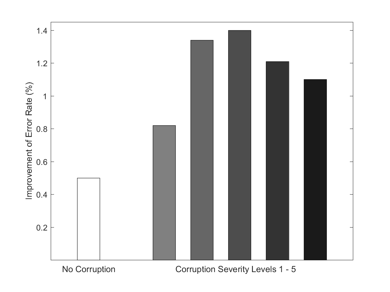
We have shown in previous experiments that OrthDNNs, particularly our proposed SVB and BBN, have better generalization to testing samples that are drawn from the same distributions of training ones. In this section, we investigate the robustness of OrthDNNs when testing samples are corrupted such that they are getting away from the distributions of training ones. We focus on corruptions that are frequently encountered in natural images, e.g., the “common” corruptions of noise, blur, weather, or digitization [24]. Existing research suggests fragility of deep learning models to corruptions of such kinds [16], and that fine-tuning on specific corruption types would help, but cannot well generalize to other types of corruptions [18, 53]. To this end, we use the ImageNet-C dataset [24] that is produced by applying 15 corruption types of 5 severity levels to validation images of ImageNet [47] ³³ 3 The 15 types of corruptions include Gaussian Noise, Shot Noise, Impulse Noise, Defocus Blur, Frosted Glass Blur, Motion Blur, Zoom Blur, Snow, Frost, Fog, Brightness, Contrast, Elastic, Pixelate, and JPEG. Refer to [24] for examples of corrupted ImageNet validation images.. As indicated in [24], networks should not be trained or fine-tuned on this dataset for testing of their robustness. We again use the trained models of ResNeXt-101 as described in section V-C, with or without the regularization of SVB and BBN. Performance improvements of top-1 error rates are plotted in fig. 5, where result for each severity level is an average over the 15 types of corruptions. Compared with the result on clean images of ImageNet validation set, fig. 5 demonstrates better robustness of our proposed methods against common corruptions, and the robustness stands gracefully with the increase of severity levels.

VI Conclusion

In this paper, we present theoretical analysis to connect with the recent interest of spectrally regularized deep learning methods. Technically, we prove a new generalization error bound for DNNs, which is both scale- and range-sensitive to singular value spectrum of each of networks’ weight matrices. The bound is established by first proving that DNNs are of local isometry on data distributions of practical interest, and then introducing the local isometry property of DNNs into a PAC based generalization analysis. We further prove that the optimal bound w.r.t. the degree of isometry is attained when each weight matrix has a spectrum of equal singular values — OrthDNNs with weight matrices of orthonormal rows or columns are thus the most straightforward choice. Based on such analysis, we present algorithms of strict and approximate OrthDNNs, and propose a simple yet effective algorithm called Singular Value Bounding. We also propose Bounded Batch Normalization to make compatible use of batch normalization with OrthDNNs. Experiments on benchmark image classification show the efficacy and robustness of OrthDNNs and our proposed SVB and BNN methods.

References

[1] P. A. Absil, R. Mahony, and R. Sepulchre. Optimization Algorithms on Matrix Manifolds. Princeton University Press, Princeton, NJ, USA, 2007.
[2] Martin Arjovsky, Amar Shah, and Yoshua Bengio. Unitary evolution recurrent neural networks. CoRR, arXiv:1511.06464, 2016.
[3] Pierre Baldi and Peter J Sadowski. Understanding dropout. In Advances in Neural Information Processing Systems 26, pages 2814–2822. 2013.
[4] Nitin Bansal, Xiaohan Chen, and Zhangyang Wang. Can we gain more from orthogonality regularizations in training deep cnns? In Proceedings of the 32Nd International Conference on Neural Information Processing Systems, NIPS’18, pages 4266–4276, 2018.
[5] Nitin Bansal, Xiaohan Chen, and Zhangyang Wang. Can we gain more from orthogonality regularizations in training deep networks? In Advances in Neural Information Processing Systems 31, pages 4261–4271. 2018.
[6] Andrew R. Barron. Universal approximation bounds for superpositions of a sigmoidal function. IEEE Transactions on Information Theory, 39(3):930–945, 1993.
[7] Peter L. Bartlett, Dylan J. Foster, and Matus J. Telgarsky. Spectrally-normalized margin bounds for neural networks. In Advances in Neural Information Processing Systems, pages 6241–6250, 2017.
[8] Gary Bécigneul. On the effect of pooling on the geometry of representations. Technical report, 2017.
[9] S. Bonnabel. Stochastic gradient descent on riemannian manifolds. IEEE Transactions on Autom. Control, 58(9):2217–2229, 2013.
[10] Olivier Bousquet and André Elisseeff. Stability and generalization. Journal of Machine Learning Research, 2:499–526, March 2002.
[11] E. J. Candes and T. Tao. Decoding by linear programming. IEEE Trans. Inf. Theor., 51(12):4203–4215, December 2005.
[12] Djalil Chafaï, Djalil Chafäı, Olivier Guédon, Guillaume Lecue, and Alain Pajor. Singular values of random matrices. https://pdfs.semanticscholar.org/37f9/fc9b8cb7a04c7863a0d53c4c3a84a8a7da64.pdf.
[13] Moustapha Cisse, Piotr Bojanowski, Edouard Grave, Yann Dauphin, and Nicolas Usunier. Parseval networks: Improving robustness to adversarial examples. In Proceedings of the 34th International Conference on Machine Learning, pages 854–863, 2017.
[14] Yann N. Dauphin, Razvan Pascanu, Çaglar Gülçehre, KyungHyun Cho, Surya Ganguli, and Yoshua Bengio. Identifying and attacking the saddle point problem in high-dimensional non-convex optimization. In Advances in Neural Information Processing Systems 27, pages 2933–2941, 2014.
[15] Laurent Dinh, Razvan Pascanu, Samy Bengio, and Yoshua Bengio. Sharp minima can generalize for deep nets. In International Conference on Machine Learning, pages 1019–1028, 2017.
[16] Samuel Dodge and Lina Karam. A study and comparison of human and deep learning recognition performance under visual distortions. arXiv preprint arXiv:1705.02498, 2017.
[17] K. Fukushima. Neocognitron: A self-organizing neural network for a mechanism of pattern recognition unaffected by shift in position. Biological Cybernetics, 36(4):193–202, 1980.
[18] R. Geirhos, D. H. J. Janssen, H. H. Schütt, J. Rauber, M. Bethge, and F. A. Wichmann. Comparing deep neural networks against humans: object recognition when the signal gets weaker. arXiv preprint arXiv:1706.06969, 2017.
[19] Xavier Glorot and Yoshua Bengio. Understanding the difficulty of training deep feedforward neural networks. In Proceedings of the International Conference on Artificial Intelligence and Statistics, 2010.
[20] Xavier Glorot, Antoine Bordes, and Yoshua Bengio. Deep sparse rectifier neural networks. In Proceedings of the International Conference on Artificial Intelligence and Statistics, 2011.
[21] Moritz Hardt, Ben Recht, and Yoram Singer. Train faster, generalize better: Stability of stochastic gradient descent. In Proceedings of The 33rd International Conference on Machine Learning, volume 48, pages 1225–1234, 2016.
[22] Kaiming He, Xiangyu Zhang, Shaoqing Ren, and Jian Sun. Deep residual learning for image recognition. In arXiv prepring arXiv:1506.01497, 2015.
[23] Kaiming He, Xiangyu Zhang, Shaoqing Ren, and Jian Sun. Identity mappings in deep residual networks. In European Conference on Computer Vision, 2016.
[24] Dan Hendrycks and Thomas Dietterich. Benchmarking neural network robustness to common corruptions and perturbations. In International Conference on Learning Representations, 2019.
[25] Geoffrey E. Hinton, Nitish Srivastava, Alex Krizhevsky, Ilya Sutskever, and Ruslan Salakhutdinov. Improving neural networks by preventing co-adaptation of feature detectors. CoRR, abs/1207.0580, 2012.
[26] K. Hornik, M. Stinchcombe, and H. White. Multilayer feedforward networks are universal approximators. Neural Networks, 2(5):359–366, 1989.
[27] Gao Huang, Zhuang Liu, and Kilian Q. Weinberger. Densely connected convolutional networks. CoRR, abs/1608.06993, 2016.
[28] Jiaji Huang, Qiang Qiu, Guillermo Sapiro, and Robert Calderbank. Discriminative robust transformation learning. In Advances in Neural Information Processing Systems 28, pages 1333–1341. 2015.
[29] Sergey Ioffe and Christian Szegedy. Batch normalization: Accelerating deep network training by reducing internal covariate shift. In Proceedings of the 32nd International Conference on Machine Learning, pages 448–456, 2015.
[30] Kui Jia, Dacheng Tao, Shenghua Gao, and Xiangmin Xu. Improving training of deep neural networks via singular value bounding. In IEEE Conference on Computer Vision and Pattern Recognition, pages 3994–4002, 2017.
[31] Kenji Kawaguchi. Deep learning without poor local minima. In Advances in Neural Information Processing Systems, 2016.
[32] Kenji Kawaguchi, Leslie Pack Kaelbling, and Yoshua Bengio. Generalization in deep learning. CoRR, abs/1710.05468, 2017.
[33] Nitish Shirish Keskar, Dheevatsa Mudigere, Jorge Nocedal, Mikhail Smelyanskiy, and Ping Tak Peter Tang. On large-batch training for deep learning: Generalization gap and sharp minima. In International Conference on Learning Representations, 2017.
[34] Diederik Kingma and Jimmy Ba. Adam: A method for stochastic optimization. In International Conference on Learning Representations, 2015.
[35] A. N. Kolmogorov and V. Tihomirov. $\epsilon$ -entropy and $\epsilon$ -capacity of sets in functional spaces. American Mathematical Society Translations (2), 17:227–364, 2002.
[36] Alex Krizhevsky. Learning multiple layers of features from tiny images. Tech. Report, 2009.
[37] Ilja Kuzborskij and Christoph H. Lampert. Data-dependent stability of stochastic gradient descent. CoRR, 1703.01678, 2017.
[38] Y. LeCun, L. Bottou, Y. Bengio, and P. Haffner. Gradient-based learning applied to document recognition. Proceedings of the IEEE, 86(11):2278–2324, 1998.
[39] Yann LeCun, Léon Bottou, Genevieve B. Orr, and Klaus-Robert Müller. Efficient backprop. In Neural Networks: Tricks of the Trade, pages 9–50, 1998.
[40] Chen-Yu Lee, Saining Xie, Patrick W. Gallagher, Zhengyou Zhang, and Zhuowen Tu. Deeply-supervised nets. In Proceedings of the Eighteenth International Conference on Artificial Intelligence and Statistics, 2015.
[41] Tongliang Liu, Gábor Lugosi, Gergely Neu, and Dacheng Tao. Algorithmic stability and hypothesis complexity. In International Conference on Machine Learning, pages 2159–2167, 2017.
[42] Mehryar Mohri, Afshin Rostamizadeh, and Ameet Talwalkar. Foundations of Machine Learning. The MIT Press, 2012.
[43] Guido Montúfar, Razvan Pascanu, Kyunghyun Cho, and Yoshua Bengio. On the number of linear regions of deep neural networks. In Advances in Neural Information Processing Systems, pages 2924–2932, 2014.
[44] P. Orlik and H. Terao. Arrangements of Hyperplanes. Grundlehren der mathematischen Wissenschaften. Springer Berlin Heidelberg, 1992.
[45] Mete Ozay and Takayuki Okatani. Optimization on submanifolds of convolution kernels in cnns. CoRR, abs/1610.07008, 2016.
[46] Jeffrey Pennington, Samuel S. Schoenholz, and Surya Ganguli. Resurrecting the sigmoid in deep learning through dynamical isometry: theory and practice. In Advances in Neural Information Processing Systems, pages 4788–4798, 2017.
[47] Olga Russakovsky, Jia Deng, Hao Su, Jonathan Krause, Sanjeev Satheesh, Sean Ma, Zhiheng Huang, Andrej Karpathy, Aditya Khosla, Michael Bernstein, Alexander C. Berg, and Li Fei-Fei. ImageNet Large Scale Visual Recognition Challenge. International Journal of Computer Vision, 115(3):211–252, 2015.
[48] Andrew M. Saxe, James L. McClelland, and Surya Ganguli. Exact solutions to the nonlinear dynamics of learning in deep linear neural networks. In International Conference on Learning Representations, 2014.
[49] Hanie Sedghi, Vineet Gupta, and Philip M. Long. The singular values of convolutional layers. In Proceedings of the International Conference on Learning and Representation (ICLR), 2019.
[50] K. Simonyan and A. Zisserman. Very deep convolutional networks for large-scale image recognition. CoRR, abs/1409.1556, 2014.
[51] Jure Sokolic, Raja Giryes, Guillermo Sapiro, and Miguel R. D. Rodrigues. Robust large margin deep neural networks. IEEE Trans. Signal Processing, 65(16):4265–4280, 2017.
[52] Ilya Sutskever, James Martens, George E. Dahl, and Geoffrey E. Hinton. On the importance of initialization and momentum in deep learning. In Proceedings of the 30th International Conference on Machine Learning, volume 28, pages 1139–1147, May 2013.
[53] Igor Vasiljevic, Ayan Chakrabarti, and Gregory Shakhnarovich. Examining the impact of blur on recognition by convolutional networks. arXiv preprint arXiv:1611.05760, 2016.
[54] Nakul Verma. Distance Preserving Embeddings for General n-Dimensional Manifolds. Journal of Machine Learning Research, 14:2415–2448, 2013.
[55] Stefan Wager, Sida Wang, and Percy S Liang. Dropout training as adaptive regularization. In Advances in Neural Information Processing Systems 26, pages 351–359. 2013.
[56] Shengjie Wang, Abdel-rahman Mohamed, Rich Caruana, Jeff A. Bilmes, Matthai Philipose, Matthew Richardson, Krzysztof Geras, Gregor Urban, and Özlem Aslan. Analysis of deep neural networks with extended data jacobian matrix. In Proceedings of the 33nd International Conference on Machine Learning, pages 718–726, 2016.
[57] Scott Wisdom, Thomas Powers, John R. Hershey, Jonathan Le Roux, and Les Atlas. Full-capacity unitary recurrent neural networks. CoRR, arXiv:1611.00035, 2016.
[58] Di Xie and Jiang Xiongand Shiliang Pu. All you need is beyond a good init: Exploring better solution for training extremely deep convolutional neural networks with orthonormality and modulation. In Computer Vision and Pattern Recognition, 2017.
[59] Saining Xie, Ross B. Girshick, Piotr Dollár, Zhuowen Tu, and Kaiming He. Aggregated residual transformations for deep neural networks. In IEEE Conference on Computer Vision and Pattern Recognition, pages 5987–5995, 2017.
[60] Huan Xu and Shie Mannor. Robustness and generalization. Machine Learning, 86(3):391–423, 2012.
[61] Chulhee Yun, Suvrit Sra, and Ali Jadbabaie. Global optimality conditions for deep neural networks. In International Conference on Learning Representations, 2018.
[62] Sergey Zagoruyko and Nikos Komodakis. Wide residual networks. CoRR, abs/1605.07146, 2016.
[63] Chiyuan Zhang, Samy Bengio, Moritz Hardt, Benjamin Recht, and Oriol Vinyals. Understanding deep learning requires rethinking generalization. In International Conference on Learning Representations, 2017.
[64] Chiyuan Zhang, Qianli Liao, Alexander Rakhlin, Brando Miranda, Noah Golowich, and Tomaso A. Poggio. Theory of deep learning iib: Optimization properties of SGD. CoRR, 1801.02254, 2018.

Appendix A Proof of Lemma 3.1.

To prove lemma III.1, we begin with the following lemma regarding matrix pseudo-inverse.

Lemma A.1.

Given a matrix $\bm{W}\in\mathbb{R}^{M\times N}$ and $\bm{x}\in\mathcal{X}-\mathcal{N}(\bm{W})$ , where $\mathcal{X}$ is $\mathbb{R}^{N}$ , we have

\bm{W}^{{\dagger}}\bm{W}\bm{x}=\bm{x}

where $\bm{W}^{{\dagger}}$ is the pseudo-inverse of $\bm{W}$ , given as $\bm{W}^{{\dagger}}=\bm{V}\bm{\Sigma}^{{\dagger}}\bm{U}^{T}$ when $\bm{W}$ has the singular value decomposition $\bm{W}=\bm{U}\bm{\Sigma}\bm{V}^{T}$ , and $\bm{\Sigma}^{{\dagger}}$ is the matrix obtained by first taking the transpose of $\bm{\Sigma}$ , and then the inverse of its non-zero elements.

Proof.

Let $\mathcal{R}$ be the index set such that $\bm{\Sigma}_{rr}\not=0$ , $\forall r\in\mathcal{R}$ . Given any $\bm{x}\in\mathcal{X}-\mathcal{N}(\bm{W})$ , $\bm{x}$ can be represented as

\bm{x}=\bm{V}\bm{\alpha},

where entries of $\bm{\alpha}$ have $\alpha_{r}=0$ when $r\not\in\mathcal{R}$ . Then

	$\displaystyle\bm{W}^{{\dagger}}\bm{Ｗ}\bm{W}\bm{x}$	$\displaystyle=\bm{V}\bm{\Sigma}^{{\dagger}}\bm{U}^{T}\bm{U}\bm{\Sigma}\bm{V}^{T}\bm{V}\bm{\alpha}$
		$\displaystyle=\bm{V}\bm{\Sigma}^{{\dagger}}\bm{\Sigma}\bm{\alpha}.$

Since $\forall\alpha_{r}\not=0$ , $\bm{\Sigma}_{rr}\not=0,\bm{\Sigma}^{{\dagger}}_{rr}\not=0$ , we have $\bm{\Sigma}^{{\dagger}}\bm{\Sigma}\bm{\alpha}=\bm{\alpha}$ , which is to say $\bm{W}^{{\dagger}}\bm{W}\bm{x}=\bm{V}\bm{\alpha}=\bm{x}$ . ∎

Now, we are going to prove lemma III.1.

Proof.

For any $\bm{W}_{i}$ with $i\in\{1,\ldots,L\}$ , performing singular value decomposition (SVD) upon it, we have

\bm{W}_{i}=\bm{U}_{i}\bm{\Sigma}_{i}\bm{V}^{T}_{i},

where $\bm{U}_{i}$ and $\bm{V}_{i}$ are both orthogonal matrices.

Given any $\bm{\Delta}=\bm{x}-\bm{x}^{\prime}\in\mathcal{X}-\mathcal{N}(T)$ , let $\bm{\Delta}_{i-1}=\prod_{j=1}^{i-1}\bm{W}_{j}\bm{\Delta}$ , we have

\bm{W}_{i}\bm{\Delta}_{i-1}=\bm{U}_{i}\bm{\Sigma}_{i}\bm{V}_{i}^{T}\bm{\Delta}_{i-1}.

Let $\bm{\Delta}^{\prime}_{i-1}=\bm{V}_{i}^{T}\bm{\Delta}_{i-1}$ . We show that if $\bm{\Delta}^{\prime}_{i-1,k}\not=0$ , then $\bm{\Sigma}_{i,kk}\not=0$ , which implies that $\bm{\Delta}_{i-1}$ lies in the subspace spanned by right singular vectors of $\bm{W}_{i}$ that have nonzero singular values, where $\bm{\Delta}^{\prime}_{i-1,k}$ and $\bm{\Sigma}_{i,kk}$ are respectively the $k^{th}$ element of $\bm{\Delta}^{\prime}_{i-1}$ and $k^{th}$ diagonal element of $\bm{\Sigma}_{i}$ .

Suppose otherwise, for a set $\mathcal{K}$ , $\bm{\Delta}^{\prime}_{i-1,k}\not=0$ and $\bm{\Sigma}_{i,kk}=0$ , $\forall k\in\mathcal{K}$ . Let $\bm{v}_{k}$ denote the $k^{th}$ column of $\bm{V}_{i}$ , we reparameterize $\bm{\Delta}_{i-1}$ as

\bm{\Delta}_{i-1}=\sum\limits_{k\not\in\mathcal{K}}\bm{\Delta}^{\prime}_{i-1,k}\bm{v}_{k}+\sum\limits_{k\in\mathcal{K}}\bm{\Delta}^{\prime}_{i-1,k}\bm{v}_{k},

where the terms having $\bm{\Delta}^{\prime}_{i-1,k}=0$ are omitted.

Denote $\bm{W}=\prod_{j=1}^{i-1}\bm{W}_{j}$ . Since $\bm{\Delta}\in\mathcal{X}-\mathcal{N}(\bm{T})$ , we have $\bm{\Delta}\in\mathcal{X}-\mathcal{N}(\bm{W})$ . By lemma A.1, we have $\bm{W}^{{\dagger}}\bm{\Delta_{i-1}}=\bm{W}^{{\dagger}}\bm{W}\bm{\Delta}=\bm{\Delta}\in\mathcal{X}-\mathcal{N}(\bm{T})$ . Since

	$\displaystyle\bm{W}^{{\dagger}}\bm{\Delta_{i-1}}$	$\displaystyle=\bm{W}^{{\dagger}}(\sum\limits_{k\not\in\mathcal{K}}\bm{\Delta}^{\prime}_{i-1,k}\bm{v}_{k}+\sum\limits_{k\in\mathcal{K}}\bm{\Delta}^{\prime}_{i-1,k}\bm{v}_{k})$
		$\displaystyle=\sum\limits_{k\not\in\mathcal{K}}\bm{\Delta}^{\prime}_{i-1,k}\bm{W}^{{\dagger}}\bm{v}_{k}+\sum\limits_{k\in\mathcal{K}}\bm{\Delta}^{\prime}_{i-1,k}\bm{W}^{{\dagger}}\bm{v}_{k},$

which is to say

\bm{\Delta}=\sum\limits_{k\not\in\mathcal{K}}\bm{\Delta}^{\prime}_{i-1,k}\bm{W}^{{\dagger}}\bm{v}_{k}+\sum\limits_{k\in\mathcal{K}}\bm{\Delta}^{\prime}_{i-1,k}\bm{W}^{{\dagger}}\bm{v}_{k}.

By assumption we have $\bm{\Delta}^{\prime}_{i-1,k}\not=0$ ; we also have $\bm{W}^{{\dagger}}\bm{v}_{k}\not=\bm{0}$ — otherwise $\bm{\Delta}^{\prime}_{i-1,k}$ would be zero, and $\bm{W}^{{\dagger}}\bm{v}_{k}\perp\bm{W}^{{\dagger}}\bm{v}_{k^{\prime}}$ , for $k\not=k^{\prime}$ ; Considering that $\bm{\Delta}\in\mathcal{X}-\mathcal{N}(\bm{T})$ , we have $\bm{W}^{{\dagger}}\bm{v}_{k}\in\mathcal{X}-\mathcal{N}(\bm{T})$ . However, we assume $\bm{\Sigma}_{i,kk}=0$ for $k\in\mathcal{K}$ , and have

\bm{T}(\sum\limits_{k\in\mathcal{K}}\bm{\Delta}^{\prime}_{i-1,k}\bm{W}^{{\dagger}}\bm{v}_{k})=\bm{0},

which implies $\bm{W}^{{\dagger}}\bm{v}_{k}\in\mathcal{N}(\bm{T})$ and leads to a contradiction. We thus prove that if $\bm{\Delta}^{\prime}_{i-1,k}\not=0$ , then $\bm{\Sigma}_{i,kk}\not=0$ .

With the above result, we can constrain the sample variation more precisely through singular values of weight matrices. To be specific, for any pair of $\bm{x}_{i-1}\in\mathcal{X}_{i-1}$ and $\bm{x}^{\prime}_{i-1}\in\mathcal{X}_{i-1}$ , we have

	$\displaystyle\|\|\bm{W}_{i}\bm{x}_{i-1}-\bm{W}_{i}\bm{x}_{i-1}^{\prime}\|\|$	$\displaystyle=\|\|\bm{W}_{i}(\bm{x}_{i-1}-\bm{x}^{\prime}_{i-1})\|\|$
		$\displaystyle=\|\|\bm{U}_{i}\bm{\Sigma}_{i}\bm{V}^{T}_{i}(\bm{x}_{i-1}-\bm{x}^{\prime}_{i-1})\|\|$
		$\displaystyle=\|\|\bm{\Sigma}_{i}\bm{V}^{T}_{i}(\bm{x}_{i-1}-\bm{x}^{\prime}_{i-1})\|\|$
		$\displaystyle\geq\|\|\sigma_{\min}^{i}\bm{I}\bm{V}^{T}_{i}(\bm{x}_{i-1}-\bm{x}^{\prime}_{i-1})\|\|$
		$\displaystyle\geq\sigma_{\min}^{i}\|\|\bm{V}^{T}_{i}(\bm{x}_{i-1}-\bm{x}^{\prime}_{i-1})\|\|$
		$\displaystyle=\sigma_{\min}^{i}\|\|(\bm{x}_{i-1}-\bm{x}^{\prime}_{i-1})\|\|,$

where the second and last equalities use the fact that an orthogonal matrix does not change the norm of operated vectors, and the two inequalities are derived based on our result that for $\bm{x}_{i-1}-\bm{x^{\prime}}_{i-1}\in\bm{\Delta}_{i-1}$ , it lies in the subspace spanned by the right singular vectors of $\bm{W}_{i}$ whose corresponding singular values are great than or equal to the nonzero $\sigma^{i}_{\min}$ .

Similarly, we have

||\bm{W}_{i}\bm{x}_{i-1}-\bm{W}_{i}\bm{x}_{i-1}^{\prime}||\leq\sigma_{\max}^{i}||(\bm{x}_{i-1}-\bm{x}^{\prime}_{i-1})||.

Denote $||\bm{x}_{i-1}-\bm{x}^{\prime}_{i-1}||$ as $d_{i}$ with $d=||\bm{x}-\bm{x}^{\prime}||$ , we have

\sigma_{\min}^{i}d_{i}\leq||\bm{W}_{i}\bm{x}_{i-1}-\bm{W}_{i}\bm{x}_{i-1}^{\prime}||\leq\sigma_{\max}^{i}d_{i}.

Cascading on all layers, we have

		$\displaystyle\prod\limits_{i=1}^{L}\sigma_{\min}^{i}d\leq\|\|\prod\limits_{i=1}^{L}\bm{W}_{i}\bm{x}-\prod\limits_{i=1}^{L}\bm{W}_{i}\bm{x}^{\prime}\|\|\leq\prod\limits_{i=1}^{L}\sigma_{\max}^{i}d$
	$\displaystyle\iff$	$\displaystyle\prod\limits_{i=1}^{L}\sigma_{\min}^{i}d\leq\|\|\bm{T}\bm{x}-\bm{T}\bm{x}^{\prime}\|\|\leq\prod\limits_{i=1}^{L}\sigma_{\max}^{i}d.$

Thus

		$\displaystyle\left\|\\|\bm{T}\bm{x}-\bm{T}\bm{x}^{\prime}\|\|-\|\|\bm{x}-\bm{x}^{\prime}\\|\right\|$
	$\displaystyle\leq$	$\displaystyle\max(\|\prod\limits_{i=1}^{L}\sigma_{\max}^{i}d-d\|,\|\prod\limits_{i=1}^{L}\sigma_{\min}^{i}d-d\|)$
	$\displaystyle\leq$	$\displaystyle\max(\|\prod\limits_{i=1}^{L}\sigma_{\max}^{i}-1\|2b,\|\prod\limits_{i=1}^{L}\sigma_{\min}^{i}-1\|2b).$

We conclude the proof by showing $\bm{T}$ is of $2b\max(|\prod\limits_{i=1}^{L}\sigma_{\max}^{i}-1|,|\prod\limits_{i=1}^{L}\sigma_{\min}^{i}-1|)$ -isometry. ∎

Appendix B Proof of Lemma 3.2.

Proof.

We proceed by induction on layer $l$ .

For $l=1$ , each row in $\bm{W}_{l}$ corresponds to a hyperplane in $\mathcal{X}$ . Thus, $\bm{W}_{l}$ imposes a hyperplane arrangement $\mathcal{A}=\{\bm{W}_{l,i}\}_{i=1,\ldots,n_{l}}$ on $\mathcal{X}$ , and is associated with an index set $\mathcal{T}(\mathcal{A},\tau)$ of the region set $\mathcal{R}(\mathcal{A})$ , where $\bm{W}_{l,i}$ denotes the $i^{th}$ row of $\bm{W}_{l}$ . Denote $a_{li}$ the neuron corresponding to a hyperplane $\bm{W}_{l,i}\in\mathcal{A}$ , we have

a_{li}(\bm{x})=\begin{cases}\bm{W}_{l,i}\bm{x}&\text{if}\ \bm{x}\in r\ \forall\ r\in\{q\in\mathcal{R}|\pi_{i}\tau(q)=1\}\\ 0&\text{otherwise},\end{cases}

i.e., $a_{li}$ is linear over regions of $\mathcal{R}$ that are active on the $i^{th}$ neuron of the layer. We then have $\mathcal{Q}_{li}=\{q\in\mathcal{R}|\pi_{i}\tau(q)=1\}$ as the support of $a_{li}$ .

To present the effect in the form of $\bm{W}_{l}$ , we have

\bm{W}^{q}_{l}=\text{ diag}(\tau(q))\bm{W}_{l},

which is a linear map over each $q\in\mathcal{Q}_{l}=\bigcup_{i=1}^{n_{l}}\mathcal{Q}_{li}$ . The case $l=1$ is proved, with $\tau_{1}=\tau$ .

Assume now for all the neurons $a_{lj}$ , $j=1,\ldots,n_{l}$ , of layer $l$ , $a_{lj}$ is a linear functional over its support $Q_{lj}$ , and is $0$ -valued otherwise. We proceed by building a new set of regions $\mathcal{Q}_{(l+1)i},i=1,\ldots,n_{l+1}$ , for layer $l+1$ , whose neurons are linear functionals over regions of $\mathcal{Q}_{(l+1)i}$ .

We separately discuss the cases of $g$ with or without max pooling.

First, when $g$ does not include max pooling, for a neuron $a_{(l+1)i}$ of layer $l+1$ , it is a functional of the form

	$\displaystyle a_{(l+1)i}$	$\displaystyle=g\sum\limits_{j=1}^{n_{l}}\bm{W}_{l+1,ij}a_{lj}$
		$\displaystyle=g\text{ pre}(a_{(l+1)i}),$

where $\bm{W}_{l+1,ij}$ is the $(i,j)$ -entry of $\bm{W}_{l+1}$ . Since $\forall q\in\bigcup_{j=1}^{n_{l}}\mathcal{Q}_{lj}$ , $a_{lj},j=1,\ldots,n_{l}$ , is a linear functional over $q$ , so is the linear combination $\text{ pre}(a_{(l+1)i})$ of them.

When $\text{ pre}(a_{(l+1)i})(\bm{x})>0\ \forall\bm{x}\in q$ , $g\text{ pre}(a_{(l+1)i})=\text{ pre}(a_{(l+1)i})$ , and $q$ is not further divided by neuron $i$ . When $\text{ pre}(a_{(l+1)i})(\bm{x})>0$ for some of $\bm{x}\in q$ , by the fact that $\text{ pre}(a_{(l+1)i})$ is a monotonous function, it splits $q$ into two regions $q_{+}$ and $q_{-}$ , where $\forall\bm{x}\in q_{+},\text{ pre}(a_{(l+1)i})(\bm{x})>0$ and $\forall\bm{x}\in q_{-},\text{ pre}(a_{(l+1)i})(\bm{x})\leq 0$ . Since $g$ sets $a_{(l+1)i}=0$ $\forall\bm{x}\in q_{-}$ , $a_{(l+1)i}$ is a linear functional over $q_{+}$ . When $\text{ pre}(a_{(l+1)i})(\bm{x})\leq 0\ \forall\bm{x}\in q$ , $q$ does not provide support for neuron $i$ , but it may support other neurons.

Consequently, neurons $a_{l+1}$ further divide the region $q$ into sub-regions, where for each region, $a_{l+1}$ is a linear map. We say the boundaries of the new set of regions as the hyperplane arrangement induced by neurons, with a alight abuse of terminology. For the newly created set of regions $\mathcal{Q}_{l+1}$ , we define the labeling function $\tau_{l+1}$ for layer $l+1$ such that for $\bm{x}\in q^{\prime}\in\mathcal{Q}_{l+1}$ , we have

\pi_{i}\tau^{\text{relu}}_{l+1}(\bm{x})=\begin{cases}1&\text{if $a_{(l+1)i}(\bm{x})>0$}\\ 0&\text{if $a_{(l+1)i}(\bm{x})\leq 0$}.\end{cases}

Since for each $q^{\prime}\in\mathcal{Q}_{l+1}$ , it is a sub-region of $q\in\mathcal{Q}_{l}$ , $q^{\prime}\in\mathcal{Q}_{l}$ holds true as well. In this case, the new set of regions are built.

For the case that $g$ includes max pooling, the neuron is of the form

	$\displaystyle a_{(l+1)i}$	$\displaystyle=\max\limits_{k\in K}(\text{ ReLU}\sum\limits_{j=1}^{n_{l}}\bm{W}_{l+1,(si+k)j}a_{lj})$
		$\displaystyle=\max\limits_{k\in K}(\text{ pre}(a_{(l+1)i})_{k}),$

where $K$ is index set of neurons being pooled with $|K|=s$ , and $\text{ pre}(a_{(l+1)i})_{k}$ denotes $\text{ ReLU}\sum\limits_{j=1}^{n_{l}}\bm{W}_{l+1,(si+k)j}a_{lj}$ .

Similarly, for each $k\in K$ , $\text{ pre}(a_{(l+1)i})_{k}$ may split $q$ into two sub-regions. Denote the boundary as $H_{k}$ if it indeed splits. $\{H_{k}\}_{k\in K}$ , together with the boundary of $q$ , forms a hyperplane arrangement $\mathcal{A}^{*}_{(l+1)i}$ induced by neurons within $q$ . Denote the set of regions in this new arrangement as $\mathcal{Q}_{(l+1)i}^{*}$ , for each $q^{*}\in\mathcal{Q}_{(l+1)i}^{*}$ , consider the set of hyperplanes $\mathcal{A}^{\prime}_{(l+1)i}=\{\text{ pre}(a_{(l+1)i})_{k}-\text{ pre}(a_{(l+1)i})_{k^{\prime}}\}_{k<k^{\prime},k,k^{\prime}\in K}$ . With a similar argument, they will create another hyperplane arrangement $\mathcal{A}^{\prime}_{(l+1)i}$ within $q^{*}$ . For $q^{\prime}\in\mathcal{Q}^{\prime}_{(l+1)i}$ , $H\in\mathcal{A}^{\prime}_{(l+1)i}$ does not have discontinuity in derivative — does not suddenly switch from constant function $0$ to non-zero linear function. Now within each $q^{\prime}$ , we impose an order on $\mathcal{A}^{*}_{(l+1)i}$ , if $\text{ pre}(a_{(l+1)i})_{k}-\text{ pre}(a_{(l+1)i})_{k^{\prime}}\geq 0$ , we say $H_{k}\geq H_{k}^{\prime}$ . Given that $K$ is a finite totally ordered set, the maximum element w.r.t. the defined order exists, and we denote its index as $k_{\max}$ . Thus, for each $q^{\prime}$ , $a_{(l+1)i}=\text{ pre}(a_{(l+1)i})_{k_{\max}}$ , which we have proved to be a linear function over $q^{\prime}$ in the ReLU case, so is $a_{li}$ . Thus similar to the ReLU only case, Max Pooling with ReLU divides $q$ into a new set of regions as well.

For the newly created set of regions $\mathcal{Q}_{l+1}$ , we have a composed labeling function

\tau_{l+1}(q)=\tau^{\max}_{l+1}(q)\tau^{\text{relu}}_{l+1}(q),

where $\tau^{\text{relu}}$ is defined as before, and

\pi_{k}\tau^{\max}_{l+1}(q)=\begin{cases}1&\text{if $k=\argmax\limits_{k\in K}a_{(l+1)k}(\bm{x}),\forall\bm{x}\in q$}\\ 0&\text{otherwise}.\end{cases}

Since for each $q^{\prime}\in\mathcal{Q}_{l+1}$ , it is a sub-region of $q\in\mathcal{Q}_{l}$ , $q^{\prime}\in\mathcal{Q}_{l}$ holds true as well. In this case, the new set of regions are built. The max pooling case is proved.

The same with the case $l=1$ , to present the effect in the form of $\bm{W}_{l}$ , denoting $\tau_{l+1}(\bm{x})=\tau^{\text{relu}}_{l+1}$ for ReLU only case, and $\tau_{l+1}(\bm{x})=\tau^{\max}_{l+1}\tau^{\text{relu}}_{l+1}$ for ReLU with Max Pooling case, we have in the ReLU only case

\bm{W}^{q}_{l+1}=\text{ diag}(\tau_{l+1}(q))\bm{W}_{l+1},

and in the ReLU and Max Pooling case,

\bm{W}^{q}_{l+1}=\bm{P}_{l+1}\text{ diag}(\tau_{l+1}(q))\bm{W}_{l+1},

which both are linear maps over $q\in\mathcal{Q}_{l+1}=\bigcup_{i=1}^{n_{l+1}}\mathcal{Q}_{(l+1)i}$ ( note that $\bm{P}_{l+1}$ is a also a linear mapping/matrix).

By induction, $\forall i\leq l+1$ , $\bm{W}^{q}_{i}$ is a linear map. Cascading the result, we have the neural network $\bm{T}$ as a linear map over $q\in\mathcal{Q}_{(l+1)}$

\bm{T}^{l+1}_{q}=\prod\limits_{i=1}^{l+1}\bm{W}^{q}_{i}.

We now finish the induction and prove that for $0<l\leq L$ , there exists a set $\mathcal{Q}_{l}$ such that $\forall q\in\mathcal{Q}_{l}$ , $\bm{T}^{l}_{q}$ is linear over $q$ . Given that we are interested in $\bm{T}^{L}_{q}$ in this paper, we drop the upper index, and denote it as

\bm{T}_{q}=\prod\limits_{i=1}^{L}\bm{W}^{q}_{i},

and the corresponding region set $Q_{L}$ is the set of regions over which $\bm{T}$ is linear. We also drop the index, and denote it as $Q$ . ∎

Appendix C Proof of Lemma 3.3.

Proof.

By lemma III.2, a set of regions $\mathcal{Q}$ exists such that for $q\in\mathcal{Q}$ , $\bm{T}_{q}$ is a linear mapping induced by $\bm{T}$ over $q$ .

For any given $\bm{x}\in\mathcal{X}$ , denote the region it belongs to as $q_{\bm{x}}$ . Let $d_{\min}=\min_{\bm{x}\in S_{m}^{(x)}}\min_{\bm{x}^{\prime}\in\partial q_{\bm{x}}}\rho(\bm{x},\bm{x}^{\prime})$ , the shortest distance from $\bm{x}$ to the boundary of $q_{\bm{x}}$ , denoted as $\partial q_{\bm{x}}$ , among all training samples. Denote by $a_{lk}$ the neuron that defines the hyperplane corresponding to the boundary that produces the shortest distance $d_{\min}$ . Note that $a_{lk}$ may exist in the intermediate network layers, i.e., $1\leq l\leq L$ , and the specific value of $l$ depends on the training set $S_{m}$ and the learned $\bm{T}$ . By Corollary 3.1., we have $\forall\{\bm{x}^{\prime}\in\mathcal{X}|\>\bm{x}+(\bm{x}^{\prime}-\bm{x})\in q_{\bm{x}}\}$ , $a_{lk|\bm{x}}(\bm{x})-a_{lk|\bm{x}}(\bm{x}^{\prime})=a_{lk|\bm{x}}(\bm{x}-\bm{x}^{\prime})$ . Thus

	$\displaystyle\|\|a_{lk\|\bm{x}}(\bm{x})-a_{lk\|\bm{x}}(\bm{x}^{\prime})\|\|$	$\displaystyle=\|\|a_{lk\|\bm{x}}(\bm{x}-\bm{x}^{\prime})\|\|$
		$\displaystyle\leq\|\|a_{lk\|\bm{x}}\|\|\|\|\bm{x}-\bm{x}^{\prime}\|\|$
		$\displaystyle=\|\|a_{lk\|\bm{x}}\|\|d_{\min}.$

Given $\bm{x}^{\prime}\in\partial q_{\bm{x}}$ , it implies $a_{lk}(\bm{x}^{\prime})=0$ , and we have a lower bound on $d_{\min}$ as

	$\displaystyle d_{\min}$	$\displaystyle\geq\frac{\|\|a_{lk\|\bm{x}}(\bm{x})-a_{lk\|\bm{x}}(\bm{x}^{\prime})\|\|}{\|\|a_{lk\|\bm{x}}\|\|}$
		$\displaystyle=\frac{\|a_{lk\|\bm{x}}(\bm{x})\|}{\|\|a_{lk\|\bm{x}}\|\|}$
		$\displaystyle\geq\frac{\|a_{lk\|\bm{x}}(\bm{x})\|}{\prod\limits_{i=1}^{l}\sigma^{i}_{\max\|\bm{x}}},$

where $\sigma^{i}_{\max|\bm{x}}$ is the maximum singular value of $\bm{W}^{q}_{i}$ for $i=1,\ldots,l$ .

Since $\bm{W}^{q}_{i}$ is a submatrix of $\bm{W}_{i}$ , by Cauchy interlacing law by rows deletion [12], we have $\sigma^{i}_{\max|\bm{x}}\leq\sigma^{i}_{\max}$ , and

d_{\min}\geq\frac{|a_{lk|\bm{x}}(\bm{x})|}{\prod\limits_{i=1}^{l}\sigma^{i}_{\max}}.

Denote $o(S_{m},\bm{T})/2=|a_{lk|\bm{x}}(\bm{x})|$ to stress the fact that it is a fixed value once $S_{m}$ and $\bm{T}$ are given, we have a lower bound

r=\frac{o(S_{m},\bm{T})/2}{\prod\limits_{i=1}^{l(S_{m},\bm{T})}\sigma^{i}_{\max}},

where we have explicitly write $l(S_{m},\bm{T})$ to emphasize the dependence of $l$ on $S_{m}$ and $\bm{T}$ . In addition, $q_{\bm{x}}\in\mathcal{Q}$ , we have $\bm{T}$ is linear over $q_{\bm{x}}$ . Consequently, a covering set of $\mathcal{X}$ with radius $r$ is found, such that within each covering ball, $\bm{T}$ is linear. Then for any given $\bm{x}\in\mathcal{X}$ and $\{\bm{x}^{\prime}\in\mathcal{X}|\>||\bm{x}-\bm{x}^{\prime}||\leq r\}$ , $\bm{x}^{\prime}\in q_{\bm{x}}$ , thus $\bm{T}\bm{x}-\bm{T}\bm{x}^{\prime}=\bm{T}_{|\bm{x}}(\bm{x}-\bm{x}^{\prime})$ . The diameter $\gamma$ of the covering ball is $2r$ . ∎

Appendix D Proof of Lemma 3.4.

Proof.

By lemma III.3, there exists a covering of $\mathcal{X}$ such that $\bm{T}$ is linear over each covering ball $B$ containing $\bm{x}\in S_{m}^{(x)}$ , denoted as $\bm{T}_{|B}$ . By lemma III.1, within such a $B$ , $\bm{T}_{|B}$ is $\delta_{|B}$ -isometry w.r.t. variation space $\mathcal{X}-\mathcal{N}(\bm{T}_{|B})$ . By Cauchy interlacing law by rows deletion [12], we have

\sigma^{i}_{\max|B}\leq\sigma^{i}_{\max},\ \sigma^{i}_{\min|B}\geq\sigma^{i}_{\min},

where $\sigma^{i}_{\min}$ and $\sigma^{i}_{\max}$ , $i=1,\ldots,L$ , are respectively the minimum and maximum singular values of weight matrices of $\bm{T}$ , and $\sigma^{i}_{\min|B}$ and $\sigma^{i}_{\max|B}$ are the corresponding ones of $\bm{T}_{|B}$ .

Some extra attentions need to be taken to deal with the $\bm{P}_{l}$ matrix introduced by max pooling. Note that in lemma III.2, $||\bm{P}_{l}\text{ diag}(\tau_{l}(q))\bm{W}_{l}\bm{x}||$ is equivalent to $||\text{ diag}(\tau_{l}(q))\bm{W}_{l}\bm{x}||$ since in computing the norm, a summation is computed anyway. Thus, the Cauchy interlacing law by row deletion applies to $\bm{W}_{l}^{q}$ with $\bm{P}_{l}$ as well.

Denote

	$\displaystyle\delta^{1}_{\|B}$	$\displaystyle=\prod\limits_{i=1}^{L}\sigma^{i}_{\max\|B},\ \delta^{2}_{\|B}=\prod\limits_{i=1}^{L}\sigma^{i}_{\min\|B},$
	$\displaystyle\delta^{1}$	$\displaystyle=\prod\limits_{i=1}^{L}\sigma^{i}_{\max},\ \delta^{2}=\prod\limits_{i=1}^{L}\sigma^{i}_{\min}.$

Anchoring the four points $\delta^{1}_{B},\delta^{2}_{|B},\delta^{1},\delta^{2}$ on the graph of $f(x)=|x-1|$ , we observe that $[\delta^{2}_{|B},\delta^{1}_{|B}]$ lies between the interval $[\delta^{2},\delta^{1}]$ . Thus we have

\max(|\delta^{1}_{|B}-1|,|\delta^{2}_{|B}-1|)\leq\max(|\delta^{1}-1|,|\delta^{2}-1|).

Since $\bm{T}_{|B}$ means $\bm{T}$ over $B$ is $\max(|\delta^{1}_{|B}-1|,|\delta^{2}_{|B}-1|)$ -isometry, which implies that it is also $\max(|\delta^{1}-1|,|\delta^{2}-1|)$ -isometry. ∎

Appendix E Proof of theorem III.1

Proof.

Similar to the proof of theorem II.1, we partition the space $\mathcal{Z}$ via the assumed $\gamma$ -cover. Since $\mathcal{X}$ is a $k$ -dimensional manifold, its covering number is upper bounded by $C_{\mathcal{X}}^{k}/\gamma^{k}$ . Let $K$ be the overall number of covering set, which is upper bounded by $|\mathcal{Y}|C_{\mathcal{X}}^{k}/\gamma^{k}$ . Denote $C_{i}$ the $i$ th covering ball, and let $N_{i}$ be the set of index of training samples that fall into $C_{i}$ . Note that $(|N_{i}|)_{i=1\ldots K}$ is an IDD multimonial random variable with parameters $m$ and $(|\mu(C_{i})|)_{i=1\ldots K}$ . Then

	$\displaystyle\|R(f\circ\bm{T})-R_{m}(f\circ\bm{T})\|$
$\displaystyle=$	$\displaystyle\|\sum\limits_{i=1}^{K}\mathbb{E}_{z\sim\mu}[\mathcal{L}(f(\bm{T}\bm{x}),y)]\mu(C_{i})-\frac{1}{m}\sum\limits_{i=1}^{m}\mathcal{L}(f(\bm{T}\bm{x}_{i}),y_{i})\|$
$\displaystyle\leq$	$\displaystyle\|\sum\limits_{i=1}^{K}\mathbb{E}_{z\sim\mu}[\mathcal{L}(f(\bm{T}\bm{x}),y)]\frac{\|N_{i}\|}{m}-\frac{1}{m}\sum\limits_{i=1}^{m}\mathcal{L}(f(\bm{T}\bm{x}_{i}),y_{i})\|$
	$\displaystyle+\|\sum\limits_{i=1}^{K}\mathbb{E}_{z\sim\mu}[\mathcal{L}(f(\bm{T}\bm{x}),y)]\mu(C_{i})-\sum\limits_{i=1}^{K}\mathbb{E}_{z\sim\mu}[\mathcal{L}(f(\bm{T}\bm{x}),y)]\frac{\|N_{i}\|}{m}\|$
$\displaystyle\leq$	$\displaystyle\|\frac{1}{m}\sum\limits_{i=1}^{K}\sum\limits_{j\in N_{i}}\max\limits_{z^{\prime}\in C_{i},\bm{x}^{\prime}-\bm{x}_{j}\in\mathcal{P}_{\bm{x}_{j}}}\|\mathcal{L}(f(\bm{T}\bm{x}^{\prime}),y^{\prime})-\mathcal{L}(f(\bm{T}\bm{x}_{j}),y_{j})\|$	(18)
	$\displaystyle+\|\max\limits_{z\in\mathcal{Z}}\|\mathcal{L}(f(\bm{T}\bm{x}),y)\|\sum\limits_{i=1}^{K}\|\frac{\|N_{i}\|}{m}-\mu(C_{i})\|\|.$	(19)

Remember that $z=(\bm{x},y)$ .

By the assumption that $\bm{T}$ is $\gamma$ -cover $\delta$ -isometry w.r.t. $\mathcal{P}_{\bm{x}}$ of $\bm{x}\in S_{m}^{(x)}$ and the Lipschitz constant of $\mathcal{L}\circ f$ is $A$ , suppose the maximum is achieved at $\bm{x}_{k}$ and $\bm{x}_{k}\in C_{p}$ , we have

	$\displaystyle\max\limits_{z^{\prime}\in C_{p},\bm{x}^{\prime}-\bm{x}_{k}\in\mathcal{P}_{\bm{x}_{k}}}\|\mathcal{L}(f(\bm{T}\bm{x}^{\prime}),y^{\prime})-\mathcal{L}(f(\bm{T}\bm{x}_{k}),y_{k})\|$
$\displaystyle\leq$	$\displaystyle A\max\limits_{z^{\prime}\in C_{p},\bm{x}^{\prime}-\bm{x}_{k}\in\mathcal{P}_{\bm{x}_{k}}}\|\|\bm{T}_{\|\bm{x}_{k}}(\bm{x}^{\prime}-\bm{x}_{k})\|\|$	(20)
$\displaystyle\leq$	$\displaystyle A\max\limits_{z^{\prime}\in C_{p},\bm{x}^{\prime}-\bm{x}_{k}\in\mathcal{P}_{\bm{x}_{k}}}(\|\|\bm{x}^{\prime}-\bm{x}_{k}\|\|+\delta)$	(21)
$\displaystyle\leq$	$\displaystyle A(\gamma+\delta),$

where $\delta=2b|\prod_{i=1}^{L}\sigma^{i}_{\max}-1|$ in (21) since we have $||\bm{T}_{|\bm{x}_{k}}(\bm{x}^{\prime}-\bm{x}_{k})||\leq||\bm{x}^{\prime}-\bm{x}_{k}||+2b|\prod_{i=1}^{L}\sigma^{i}_{\max}-1|$ by Lemma III.1, and $\gamma=o(S_{m},\bm{T})/\left(\prod\limits_{i=1}^{l(S_{m},\bm{T})}\sigma^{i}_{\max}\right)>0$ by Lemma III.3, with values of $o(S_{m},\bm{T})$ and $1\leq l(S_{m},\bm{T})\leq L$ depending on the training set $S_{m}$ and learned network $\bm{T}$ . Thus eq. 18 is less than or equal to $A(\gamma+\delta)$ with the specified $\gamma$ and $\delta$ . By Breteganolle-Huber-Carol inequality, eq. 19 is less than or equal to $M\sqrt{\frac{\log(2)|\mathcal{Y}|2^{k+1}C_{\mathcal{X}}^{k}}{\gamma^{k}n}+\frac{2\log(1/\nu)}{m}}$ .

The proof is finished. Note that given the covering number of $\mathcal{X}$ as $\mathcal{N}=(\frac{C_{\mathcal{X}}}{\gamma/2})^{k}$ , we have also proved that the algorithm is $(|\mathcal{Y}|\mathcal{N},A(\gamma+\delta))$ -robust. ∎

Appendix F

In this section, we present a SGD based algorithm for the constrained optimization problem (i.e. problem (IV-A)) of training a DNN of $L$ layers with parameters $\Theta=\{\mathbf{W}_{l},\mathbf{b}_{l}\}_{l=1}^{L}$ and objective function ${\cal{L}}$ . The constraints enforce the weight matrix (kernel) $\mathbf{W}_{l}\in\mathbb{R}^{n_{l}\times n_{l-1}}$ of any $l^{th}$ layer of the network staying on the Stiefel manifold defined as ${\cal{M}}_{l}=\{\mathbf{W}_{l}\in\mathbb{R}^{n_{l}\times n_{l-1}}|\mathbf{W}_{l}^{\top}\mathbf{W}_{l}=\mathbf{I}\}$ , assuming $n_{l}\geq n_{l-1}$ . The presented algorithm applies directly to fully-connected network layers. For convolutional layers used in CNNs, one may refer to section IV-E for how to convert their layer kernels as matrices.

For the $t^{th}$ iteration of SGD, the algorithm performs the following sequential steps to update $\mathbf{W}^{t}_{l}\in{\cal{M}}_{l}$ for the $l^{th}$ network layer with $l\in\{1,\dots,L\}$ . Updating of other network parameters such as bias vectors $\{\mathbf{b}_{l}\}_{l=1}^{L}$ is the same as standard SGD based methods. The algorithm is similar to those of optimization on matrix manifolds in [1, 9, 45], where properties of convergence are also analyzed.

1.

Compute the gradient $\frac{\partial{\cal{L}}}{\partial{\mathbf{W}^{t}_{l}}}$ in the embedding Euclidean space via back-propagation. One may alternatively use the momentum [52] to replace the gradient term in the following steps.
2.

Project $\frac{\partial{\cal{L}}}{\partial{\mathbf{W}^{t}_{l}}}$ (or its momentum version) onto the tangent space $T_{\mathbf{W}^{t}_{l}}{\cal{M}}_{l}$ by ${\cal{P}}_{\mathbf{W}^{t}_{l}}\frac{\partial{\cal{L}}}{\partial{\mathbf{W}^{t}_{l}}}$ , to obtain the manifold gradient $\Omega_{\mathbf{W}^{t}_{l}}$ . For the considered Stiefel manifold, the tangent space at $\mathbf{W}^{t}_{l}$ is defined as $T_{\mathbf{W}^{t}_{l}}{\cal{M}}_{l}=\{\mathbf{Z}\in\mathbb{R}^{n_{l}\times n_{l-1}}|\mathbf{W}_{l}^{t\top}\mathbf{Z}+\mathbf{Z}^{\top}\mathbf{W}^{t}_{l}=0\}$ , and the projection operator is defined as ${\cal{P}}_{\mathbf{W}^{t}_{l}}\frac{\partial{\cal{L}}}{\partial{\mathbf{W}^{t}_{l}}}=\left(\mathbf{I}-\mathbf{W}^{t}_{l}\mathbf{W}_{l}^{t\top}\right)\frac{\partial{\cal{L}}}{\partial{\mathbf{W}^{t}_{l}}}+\frac{1}{2}\mathbf{W}^{t}_{l}\left(\mathbf{W}_{l}^{t\top}\frac{\partial{\cal{L}}}{\partial{\mathbf{W}^{t}_{l}}}-\frac{\partial{\cal{L}}}{\partial{\mathbf{W}^{t}_{l}}}^{\top}\mathbf{W}^{t}_{l}\right)$ , where $\mathbf{I}$ is the identity matrix of compatible size.
3.

Update $\mathbf{W}^{t}_{l}$ as $\mathbf{W}^{t}_{l}-\eta^{t}\Omega_{\mathbf{W}^{t}_{l}}$ with the step size $\eta^{t}$ that satisfies conditions of convergence [1, 9].
4.

Perform the retraction ${\cal{R}}_{\mathbf{W}^{t}_{l}}(-\eta^{t}\Omega_{\mathbf{W}^{t}_{l}})$ that defines a mapping from the tangent space to the Stiefel manifold, and update $\mathbf{W}^{t}_{l}$ as $\mathbf{W}^{t+1}_{l}={\cal{R}}_{\mathbf{W}^{t}_{l}}(-\eta^{t}\Omega_{\mathbf{W}^{t}_{l}})$ . The retraction is achieved by ${\cal{R}}_{\mathbf{W}^{t}_{l}}(-\eta^{t}\Omega_{\mathbf{W}^{t}_{l}})={\cal{Q}}(\mathbf{W}^{t}_{l}-\eta^{t}\Omega_{\mathbf{W}^{t}_{l}})$ , where the operator ${\cal{Q}}$ denotes the Q factor of the QR matrix decomposition. QR decomposition can be computed using Gram-Schmidt orthonormalization.

Appendix G Proof of Lemma 4.1

Proof.

We first consider the general case, and let $P=\min(M,N)$ . Denote singular values of $\mathbf{W}$ as $\sigma_{1}=\cdots=\sigma_{P}=1$ , and singular values of $\widetilde{\mathbf{W}}$ as $\tilde{\sigma}_{1}\geq\cdots\geq\tilde{\sigma}_{P}$ . Based on the properties of matrix extreme singular values, we have

\displaystyle\sigma_{1}=\|\mathbf{W}\|_{2}=\max_{\mathbf{x}\neq 0}\frac{\|\mathbf{W}\mathbf{x}\|_{2}}{\|\mathbf{x}\|_{2}}=\min_{\mathbf{x}\neq 0}\frac{\|\mathbf{W}\mathbf{x}\|_{2}}{\|\mathbf{x}\|_{2}}=\sigma_{P}=1.

Let $\mathbf{x}^{*}=\arg\max_{\mathbf{x}\neq 0}\frac{\|\widetilde{\mathbf{W}}\mathbf{x}\|_{2}}{\|\mathbf{x}\|_{2}}$ , we have

\displaystyle\tilde{\sigma}_{1}=\frac{\|\widetilde{\mathbf{W}}\mathbf{x}^{*}\|_{2}}{\|\mathbf{x}^{*}\|_{2}}=\frac{\|\mathbf{G}\mathbf{W}\mathbf{x}^{*}\|_{2}}{\|\mathbf{x}^{*}\|_{2}}\leq\frac{\|\mathbf{G}\|_{2}\|\mathbf{W}\mathbf{x}^{*}\|_{2}}{\|\mathbf{x}^{*}\|_{2}},

where we have used the fact that $\|\mathbf{A}\mathbf{b}\|_{2}\leq\|\mathbf{A}\|_{2}\|\mathbf{b}\|_{2}$ for any $\mathbf{A}\in\mathbb{R}^{m\times n}$ and $\mathbf{b}\in\mathbb{R}^{n}$ . We thus have

\displaystyle\tilde{\sigma}_{1}\leq\|\mathbf{G}\|_{2}\frac{\|\mathbf{W}\mathbf{x}^{*}\|_{2}}{\|\mathbf{x}^{*}\|_{2}}\leq\|\mathbf{G}\|_{2}\max_{\mathbf{x}\neq 0}\frac{\|\mathbf{W}\mathbf{x}\|_{2}}{\|\mathbf{x}\|_{2}}=|g_{\max}|.

Since $\mathbf{G}$ has nonzero entries, we have $\mathbf{W}=\mathbf{G}^{-1}\widetilde{\mathbf{G}}$ . Let $\mathbf{x}^{*}=\arg\min_{\mathbf{x}\neq 0}\frac{\|\widetilde{\mathbf{W}}\mathbf{x}\|_{2}}{\|\mathbf{x}\|_{2}}$ , the properties of matrix extreme singular values give $\tilde{\sigma}_{P}=\frac{\|\widetilde{\mathbf{G}}\mathbf{x}^{*}\|_{2}}{\|\mathbf{x}^{*}\|_{2}}$ , and $\sigma_{P}=\min_{\mathbf{x}\neq 0}\frac{\|\mathbf{W}\mathbf{x}\|_{2}}{\|\mathbf{x}\|_{2}}=1$ . We thus have

\displaystyle 1=\min_{\mathbf{x}\neq 0}\frac{\|\mathbf{G}^{-1}\widetilde{\mathbf{G}}\mathbf{x}\|_{2}}{\|\mathbf{x}\|_{2}}\leq\frac{\|\mathbf{G}^{-1}\widetilde{\mathbf{G}}\mathbf{x}^{*}\|_{2}}{\|\mathbf{x}^{*}\|_{2}}\leq\|\mathbf{G}^{-1}\|_{2}\frac{\|\widetilde{\mathbf{G}}\mathbf{x}^{*}\|_{2}}{\|\mathbf{x}^{*}\|_{2}},

which gives $\tilde{\sigma}_{P}\geq|g_{\min}|$ . Overall, we have

\displaystyle|g_{\max}|\geq\tilde{\sigma}_{1}\geq\cdots\geq\tilde{\sigma}_{P}\geq|g_{\min}|.

We next consider the special case of $M\leq N$ and $\textrm{rank}(\mathbf{W})=M$ . Without loss of generality, we assume diagonal entries $\{g_{i}\}_{i=1}^{M}$ of $\mathbf{G}$ are all positive and ordered. By definition we have $\widetilde{\mathbf{W}}=\mathbf{I}\mathbf{G}\mathbf{W}$ , where $\mathbf{I}$ is an identity matrix of size $M\times M$ . Let $\mathbf{V}=\left[\mathbf{W}^{\top},\mathbf{W}^{\bot\top}\right]$ , where $\mathbf{W}^{\bot}$ denotes the orthogonal complement of $\mathbf{W}$ , we thus have the SVD of $\widetilde{\mathbf{W}}$ by construction as $\widetilde{\mathbf{W}}=\mathbf{I}\left[\mathbf{G},\mathbf{0}\right]\mathbf{V}^{\top}$ . When some values of $\{g_{i}\}_{i=1}^{M}$ are not positive, the SVD can be constructed by changing the signs of the corresponding columns of either $\mathbf{I}$ or $\mathbf{V}$ . Since matrix singular values are uniquely determined (while singular vectors are not), singular values of $\widetilde{\mathbf{W}}$ are thus exactly $\{|g_{i}|\}_{i=1}^{M}$ . ∎

	$\displaystyle\|R(f\bm{T})-R_{m}(f\bm{T})\|$
$\displaystyle=$	$\displaystyle\|\sum\limits_{i=1}^{K}\mathbb{E}_{z\sim\mu}[\mathcal{L}(f(\bm{Tx}),y)\|z\in C_{i}]\mu(C_{i})-\frac{1}{m}\sum\limits_{i=1}^{m}\mathcal{L}(f(\bm{Tx}_{i}),y_{i})\|$
$\displaystyle\leq$	$\displaystyle\|\sum\limits_{i=1}^{K}\mathbb{E}_{z\sim\mu}[\mathcal{L}(f(\bm{Tx}),y)\|z\in C_{i}]\frac{\|N_{i}\|}{m}-\frac{1}{m}\sum\limits_{i=1}^{m}\mathcal{L}(f(\bm{Tx}_{i}),y_{i})\|$
	$\displaystyle+\|\sum\limits_{i=1}^{K}\mathbb{E}_{z\sim\mu}[\mathcal{L}(f(\bm{Tx}),y)\|z\in C_{i}]\mu(C_{i})$
	$\displaystyle\ \ \ \ \ \ \ \ \ \ \ \ \ \ \ \ -\sum\limits_{i=1}^{K}\mathbb{E}_{z\sim\mu}[\mathcal{L}(f(\bm{Tx}),y)\|z\in C_{i}]\frac{\|N_{i}\|}{m}\|$
$\displaystyle\leq$	$\displaystyle\|\frac{1}{m}\sum\limits_{i=1}^{K}\sum\limits_{j\in N_{i}}\max\limits_{z^{\prime}\in C_{i},\bm{x}^{\prime}-\bm{x}_{j}\in\mathcal{P}_{\bm{x}_{j}}}\|\mathcal{L}(f(\bm{Tx}^{\prime}),y^{\prime})-\mathcal{L}(f(\bm{Tx}_{j}),y_{j})\|\|$	(7)
	$\displaystyle\ \ \ \ \ \ \ \ \ +\|\max\limits_{z\in\mathcal{Z}}\|\mathcal{L}(f(\bm{Tx}),y)\|\sum\limits_{i=1}^{K}\|\frac{\|N_{i}\|}{m}-\mu(C_{i})\|\|.$	(8)

		$\displaystyle\max\limits_{z^{\prime}\in C_{p},\bm{x}^{\prime}-\bm{x}_{k}\in\mathcal{P}_{\bm{x}_{k}}}\|\mathcal{L}(f(\bm{Tx}^{\prime}),y^{\prime})-\mathcal{L}(f(\bm{Tx}_{k}),y_{k})\|$
		$\displaystyle=\max\limits_{z^{\prime}\in D_{z_{k}}}\|\mathcal{L}(f(\bm{Tx}^{\prime}),y^{\prime})-\mathcal{L}(f(\bm{Tx}_{k}),y_{k})\|$		(11)
		$\displaystyle\leq\text{PE}(2b\max(\|\prod_{i=1}^{L}\sigma^{i}_{\max}-1\|,\|\prod_{i=1}^{L}\sigma^{i}_{\min}-1\|)),$

	$\displaystyle\|\|\bm{W}_{i}\bm{x}_{i-1}-\bm{W}_{i}\bm{x}_{i-1}^{\prime}\|\|$	$\displaystyle=\|\|\bm{W}_{i}(\bm{x}_{i-1}-\bm{x}^{\prime}_{i-1})\|\|$
		$\displaystyle=\|\|\bm{U}_{i}\bm{\Sigma}_{i}\bm{V}^{T}_{i}(\bm{x}_{i-1}-\bm{x}^{\prime}_{i-1})\|\|$
		$\displaystyle=\|\|\bm{\Sigma}_{i}\bm{V}^{T}_{i}(\bm{x}_{i-1}-\bm{x}^{\prime}_{i-1})\|\|$
		$\displaystyle\geq\|\|\sigma_{\min}^{i}\bm{I}\bm{V}^{T}_{i}(\bm{x}_{i-1}-\bm{x}^{\prime}_{i-1})\|\|$
		$\displaystyle\geq\sigma_{\min}^{i}\|\|\bm{V}^{T}_{i}(\bm{x}_{i-1}-\bm{x}^{\prime}_{i-1})\|\|$
		$\displaystyle=\sigma_{\min}^{i}\|\|(\bm{x}_{i-1}-\bm{x}^{\prime}_{i-1})\|\|,$

		$\displaystyle\left\|\\|\bm{T}\bm{x}-\bm{T}\bm{x}^{\prime}\|\|-\|\|\bm{x}-\bm{x}^{\prime}\\|\right\|$
	$\displaystyle\leq$	$\displaystyle\max(\|\prod\limits_{i=1}^{L}\sigma_{\max}^{i}d-d\|,\|\prod\limits_{i=1}^{L}\sigma_{\min}^{i}d-d\|)$
	$\displaystyle\leq$	$\displaystyle\max(\|\prod\limits_{i=1}^{L}\sigma_{\max}^{i}-1\|2b,\|\prod\limits_{i=1}^{L}\sigma_{\min}^{i}-1\|2b).$

	$\displaystyle\|\|a_{lk\|\bm{x}}(\bm{x})-a_{lk\|\bm{x}}(\bm{x}^{\prime})\|\|$	$\displaystyle=\|\|a_{lk\|\bm{x}}(\bm{x}-\bm{x}^{\prime})\|\|$
		$\displaystyle\leq\|\|a_{lk\|\bm{x}}\|\|\|\|\bm{x}-\bm{x}^{\prime}\|\|$
		$\displaystyle=\|\|a_{lk\|\bm{x}}\|\|d_{\min}.$

Orthogonal Deep Neural Networks

Abstract

Index Terms:

I Introduction

I-A Relations with existing works

I-A1 Generalization analysis of DNNs

I-A2 Compositional computations and isometries of DNNs

I-A3 Optimization benefits of isometry/orthogonality

I-A4 Regularization on weight matrices

I-B Contributions

II Problem Statement

II-A The classification-representation-learning problem and its generalization error

II-B Generalization analysis for robust algorithms with isometric mapping

Definition 1 ((K,ϵ⁡(⋅))(K,\epsilon(\cdot))-robustness).

Theorem II.1 ([60]).

Definition 2 (Covering number).

Definition 3 (δ\delta-isometry).

Theorem II.2.

Remark.

Remark.

II-C Notations of deep neural networks

III Generalization bounds of deep neural networks

III-A δ\delta-isometry in deep neural networks

Definition 4 (Variation subspace of an instance).

Definition 5 (δ\delta-isometry w.r.t. variation subspace of an instance).

Example 1.

Lemma III.1.

Definition 6 ((Finite) Hyperplane arrangement).

Definition 7 (Region).

Definition 8 (Neuron).

Definition 9 (Support of Neuron/DNN).

Lemma III.2.

Remark.

Remark.

Corollary III.1.

Definition 10 (Linear neural network and neuron induced at 𝒙∈𝒳\bm{x}\in\mathcal{X} from a nonlinear neural network).

Definition 11 (Linear neural network and neuron induced at subset B⊂𝒳B\subset\mathcal{X} from a nonlinear neural network).

Lemma III.3.

Definition 12 (γ\gamma-cover δ\delta-isometry w.r.t. variation subspace of instance).

Lemma III.4.

Example 2.

III-B Main results of generalization bound

Theorem III.1.

Proof.

Definition 13 (Pairwise error function).

Theorem III.2.

Proof.

III-C Suggestion of new algorithms

Lemma III.5.

Proof.

IV Algorithms of Orthogonal Deep Neural Networks

IV-A The case of strict orthogonality

IV-B Achieving near orthogonality via Singular Value Bounding

IV-C Alternative algorithms for approximate OrthDNNs

IV-D Compatibility with Batch Normalization

Lemma IV.1.

IV-E Orthogonal Convolutional Neural Networks

V Experiments

V-A Comparative studies on algorithms of strict and approximate OrthDNNs

V-B Comparison of hard and soft regularization for approximate OrthDNNs

V-C Experiments with Modern Architectures

V-D Effects of Varying Sample Sizes

V-E Robustness against Common Corruptions

VI Conclusion

References

Appendix A Proof of Lemma 3.1.

Lemma A.1.

Proof.

Proof.

Appendix B Proof of Lemma 3.2.

Proof.

Appendix C Proof of Lemma 3.3.

Proof.

Appendix D Proof of Lemma 3.4.

Proof.

Appendix E Proof of theorem III.1

Proof.

Appendix F

Appendix G Proof of Lemma 4.1

Proof.

Definition 1 ( $(K,\epsilon(\cdot))$ -robustness).

Definition 3 ( $\delta$ -isometry).

III-A $\delta$ -isometry in deep neural networks

Definition 5 ( $\delta$ -isometry w.r.t. variation subspace of an instance).

Definition 10 (Linear neural network and neuron induced at $\bm{x}\in\mathcal{X}$ from a nonlinear neural network).

Definition 11 (Linear neural network and neuron induced at subset $B\subset\mathcal{X}$ from a nonlinear neural network).

Definition 12 ( $\gamma$ -cover $\delta$ -isometry w.r.t. variation subspace of instance).