Gauging fractons: immobile non-Abelian quasiparticles, fractals,
and position-dependent degeneracies
Abstract
The study of gapped quantum many-body systems in three spatial dimensions has uncovered the existence of quantum states hosting quasiparticles that are confined, not by energetics but by the structure of local operators, to move along lower dimensional submanifolds. These so-called “fracton” phases are beyond the usual topological quantum field theory description, and thus require new theoretical frameworks to describe them. Here we consider coupling fracton models to topological quantum field theories in (3+1) dimensions by starting with two copies of a known fracton model and gauging the symmetry that exchanges the two copies. This yields a class of exactly solvable lattice models that we study in detail for the case of the X-cube model and Haah’s cubic code. The resulting phases host finite-energy non-Abelian immobile quasiparticles with robust degeneracies that depend on their relative positions. The phases also host non-Abelian string excitations with robust degeneracies that depend on the string geometry. Applying the construction to Haah’s cubic code in particular provides an exactly solvable model with finite energy yet immobile non-Abelian quasiparticles that can only be created at the corners of operators with fractal support.
I Introduction
The last several decades in condensed matter physics has seen substantial progress in our understanding of gapped quantum many-body systems, ranging from topologically ordered systemsWen 2004, such as fractional quantum Hall states and quantum spin liquids, to symmetry protected topological states, such as topological insulators. While such phases can be described through the framework of topological quantum field theory (TQFT), it has more recently been understood that in three and higher spatial dimensions there are also possible gapped states that are beyond the usual TQFT description. These statesChamon 2005; Castelnovo et al. 2010; Bravyi et al. 2011; Haah 2011; Bravyi and Haah 2013; Haah 2013; Yoshida 2013; Vijay et al. 2015; Vijay et al. 2016; Nandkishore and Hermele 2018, which are now referred to as having “fracton order,” share a number of features in common with more conventional topological orders, including topologically non-trivial quasiparticle excitations and robust topology-dependent ground state degeneracies.
In contrast to conventional topological orders, fracton phases possess a strong geometry dependence, most notably in that local operators can create or destroy excitations only in certain geometric patterns, which implies that the mobility of excitations is highly constrained. For example, quasiparticles may be confined to move along certain lower dimensional submanifolds, or perhaps may even be completely immobile, despite the energy of a state with well-separated quasiparticles being finite. Importantly, these restrictions do not arise from energetics, but rather from the structure of local operators in the Hilbert space. Particles that are fully immobile are referred to as fractons. Such mobility restrictions can also occur for electric and magnetic charges in gapless gauge theoriesPretko 2017; Bulmash and Barkeshli 2018a; Gromov 2018, though we focus on the gapped case.
Since the original fracton model by ChamonChamon 2005; Bravyi et al. 2011 was presented, an intriguing development was the discovery that there are states, such as the ground states of Haah’s cubic codeHaah 2011 and several othersHsieh and Halász 2017; Tian and Wang 2019; Haah 2014, that do not support any mobile topologically non-trivial quasi-particles; in other words, the system does not support any string operator that creates a pair of quasiparticles at its ends. Instead, in Haah’s code the well-separated non-trivial quasiparticles can only be created at the corners of “fractal operators,” which are operators with support on a fractal subsystem.
These developments raise the question of how to develop a general theoretical framework to describe the set of allowed gapped states in (3+1) dimensions. Given the rich mathematical structure of topological quantum field theory and in particular the understanding of unitary modular tensor categories for (2+1) dimensional states, it is possible that the understanding of gapped fracton orders may similarly uncover a rich mathematical structure.
The Hamiltonians for Chamon’s model and Haah’s code both consist entirely of Pauli operators. Ref. Haah 2013 has since provided a classification of commuting Pauli Hamiltonians, and there has been a flurry of recent activitySlagle and Kim 2017; Slagle and Kim 2018; Shirley et al. 2018a; Slagle et al. 2018; Devakul et al. 2018; Shi and Lu 2018; Ma et al. 2018a; Shirley et al. 2019a; Schmitz et al. 2018; Halász et al. 2017; Prem et al. 2018a; Siva and Yoshida 2017; Prem et al. 2017; Bulmash and Barkeshli 2018b; Ma et al. 2018b; Shirley et al. 2018b; Shirley et al. 2018c; Bulmash and Iadecola 2019; You and von Oppen 2018; Slagle et al. 2019; Wang et al. 2019 studying various aspects of the possible fracton phases of matter. Since commuting Pauli Hamiltonians can only give rise to Abelian topological quasiparticles, which have a unique fusion outcome when fused with themselves, a natural challenge is to understand models that can give rise to non-Abelian fractons. Such phases would arise from Hamiltonians that are necessarily beyond the commuting Pauli Hamiltonian classification.
To date, there have been two approaches to developing fracton models with non-Abelian quasiparticles. The first is through a layer constructionMa et al. 2017; Vijay 2017; Vijay and Fu 2017; Prem et al. 2018b, where layers of non-Abelian (2+1)D topological orders are stacked and subsequently strings of particles from different layers are condensed in various geometrical patterns. However in this approach, in all known cases the non-Abelian quasiparticles are mobile in at least one direction. The second approachSong et al. 2018 proceeds by considering generalized gauge theories with Abelian gauge group, but combined with an analog of a Dijkgraaf-Witten cohomological twist, which renders the excitations non-Abelian. In this latter approach, immobile non-Abelian quasiparticles can be created at the corners of membrane operators. To date, phases containing immobile non-Abelian quasiparticles that can only be created by fractal operators have not been found.
A powerful way of obtaining conventional non-Abelian topological order from Abelian topological order is to gauge a global symmetry that permutes quasiparticle typesBarkeshli and Wen 2011; Barkeshli and Wen 2010; Barkeshli and Wen 2012; Barkeshli et al. 2014; Teo et al. 2015, such as the permutation symmetry of multiple copies of a topological phase. After gauging, any quasiparticle with a non-trivial orbit under the symmetry becomes non-Abelian, as are the fluxes of the symmetry (the twist defects). It is well-known that gauging subsystem symmetries of more conventional phases can produce fracton phasesVijay et al. 2016; Williamson 2016; Kubica and Yoshida 2018; Shirley et al. 2019b, and fracton phases in the presence of additional symmetriesPretko and Radzihovsky 2018; You et al. 2018 and symmetry defectsYou 2019 are an active area of current research. It is a natural question, then, to ask whether gauging a global symmetry of an Abelian fracton phase produces non-Abelian fractons.
In this paper, we consider coupling fracton phases to topological quantum field theories by gauging the permutation symmetry of multiple copies of a given fracton phase. Such a construction allows us to obtain an exactly solvable model where we couple copies of a fracton phase to any discrete gauge theory, where is a subgroup of the permutation group on copies, although we specialize to . The interplay of fracton order and topological order is an interesting topic, as it is not a priori clear whether, for example, the subdimensional excitations of the fracton system would survive when coupled in a non-trivial way to a system with topologically non-trivial mobile, deconfined excitations. We find that gauging global symmetries of Abelian fracton models indeed leads to models with non-Abelian subdimensional excitations. Notably, the gauging procedure does not affect the mobility of the excitations of the ungauged theory. Gauging symmetries in models with immobile excitations, including fractons created at the corners of fractal operators, leads to non-Abelian immobile excitations created by operators with similar support. We show explicitly that the robust degeneracy associated with these excitations depends in a highly nontrivial way on the relative positions of those excitations. The models we construct, which are based on the X-cube modelCastelnovo et al. 2010; Vijay et al. 2016 and Haah’s code, have another unusual feature: flexible, dynamical string-like excitations which carry topological degeneracy which depends on the geometry of the string. This is in contrast to conventional topological order, where the degeneracy associated to string excitations is independent of their geometry.
Our work, in particular a non-Abelian extension of Haah’s code, may also be of interest for quantum information applications. Our model allows the encoding of topologically protected degeneracy in fully immobile excitations (a benefit unique to fractons), with some logical operations on the degenerate manifold implemented via a fractonic analog of braiding. This is in contrast to Haah’s original code, where qubits would have to be encoded in the ground state subspace of the system on a topologically nontrivial manifold such as a three-torus.
The structure of this paper is as follows. In Sec. II, we explain the gauging procedure in a more familiar context by gauging the layer-swap symmetry in the bilayer (2+1)D toric code. Although the results are already well-understood from the perspective of topological order, we go into considerable detail because the technical framework is precisely the same as the one which we use in Sec. III to gauge the layer-swap symmetry of the bilayer X-Cube model. We then use Sec. IV to discuss some of the phenomenology of the gauged bilayer X-Cube model, including computing topological degeneracies and non-Abelian fracton braiding-like procedures. In Sec. V, we apply the gauging procedure to gauge the layer-swap symmetry of the bilayer Haah’s code model. Finally, Sec. VI contains discussion and conclusions. Exhaustive lists of properties of our models and some technical calculations are relegated to several appendices.
II Warmup: Gauging the (2+1)D Bilayer Toric Code
In this section, we will gauge the layer-swap symmetry of the bilayer toric code to obtain a model with the same topological order as the quantum double model (here is the symmetry group of a square). Although the resulting topological order is well-understood, at least at an abstract level, understanding the procedure in detail and at the level of explicit exactly solvable Hamiltonians generalizes directly to the fracton models. As such, it is useful to study this example in considerable depth before considering the fracton case.
Before proceeding, we comment that, at the level of exactly solvable models, there are several ways in which the gauging procedure can be performed. One method explicitly reproduces the quantum double modelKitaev 2003. Although such a result is desirable and natural for (2+1)D topological order, the required procedure does not appear to generalize easily to the (higher dimensional) fracton models, so we relegate that choice of gauging procedure to Appendix A and instead implement a gauging procedure that leads to a more convenient generalization.
II.1 Building the model
We start from two copies of the usual toric code. The Hilbert space for the ungauged model is two qubits per link of the square lattice, with ungauged Hamiltonian
| (1) | ||||
| (2) |
Here and are the usual star and plaquette operators shown in Fig. 1. As usual, and are Pauli operators. The ungauged Hamiltonian has the global symmetry , where SWAP is the local two-spin operator which exchanges the state of a single spin in layer 1 with the spin on the same link in layer 2, and the tensor product is over all links. In order to gauge the symmetry, we introduce extra “gauge” spins and modify the Hamiltonian so that some operator involving SWAP on a single link commutes with every term in the new Hamiltonian.
First we decompose the Hamiltonian into terms of definite parity under local SWAPs. The decomposition is done using the operators for . In what follows, we will need the following algebraic facts about with :
| (3) |
One can check straightforwardly that
| (4) |
where . The product is over the four different edges in a plaquette, and the condition in the sum enforces an even number of minus signs; see Fig. 2a. We have suppressed the explicit position index on the operators. An even number of minus signs is required to maintain invariance under the global SWAP operation.
We implement the gauging procedure by adding “gauge” qubits which live halfway between nearest neighbor “matter” qubits as shown in Fig. 2b. We then define the gauge symmetry generator
| (5) |
Here is an edge of the lattice of spins and the product of is taken over the four gauge spins surrounding that edge. This operator is shown in Fig. 2c. We also define the flux operator on both the sites and plaquettes of the original (matter) lattice by
| (6) |
where the product is over the four gauge spins surrounding a site or within a plaquette. We demand that generate a gauge symmetry by modifying every term in the Hamiltonian (using s) so that they commute with all . For example, the term with four signs in Fig. 2a commutes with all the and is unmodified, while the other terms in Fig. 2d require s next to every (since anticommutes with SWAP). The gauged Hamiltonian has the form
| (7) |
Here and are the gauge-invariant versions of the star and plaquette terms from the original bilayer model and are each the sum of eight terms, three of which are shown in Fig. 2d. As before, is the local symmetry generator shown in Fig. 2c; we enforce this gauge symmetry energetically. The flux term energetically penalizes the presence of flux.
II.2 Algebraic properties of
The Hamiltonian is not a stabilizer model. Nevertheless, it has considerable structure. First, it is straightforward to check that
| (8) |
This operator has eigenvalues and , so has eigenvalues and 0. The same sort of computation holds for .

Furthermore,
| (9) |
To understand this fact when and have overlapping support, we isolate single terms in each of and ; consider, for example, the product of one plaquette term, which we call , and one star term, which we call , which have only operators, as shown in Fig. 3. Using the algebraic properties in Eq. (3), it is straightforward to check that
| (10) | ||||
| (11) | ||||
| (12) |
where in the last line we simply inserted . This equation is shown pictorially in Fig. 3. Here the numbers in the subscript indicate labels for links. This is a product of a different term in with a different term in ; in commuting these operators past each other, the terms in the Hamiltonian have been permuted. Using a similar computation for each term, it is easy to check that indeed .
By construction, both and commute with every individual summand in and and with each other. Therefore, although and are not projectors, all four types of terms in the Hamiltonian commute.
II.3 String-net wavefunction picture
We now describe a simple string-net wavefunction picture for the ground states of the gauged bilayer toric code which will be convenient to use both for computing the ground state degeneracy and for understanding its excitations.
The ground states of the toric code can be understood as condensates of closed strings on (say) the links of the lattice; that is, a superposition of all possible closed strings on the lattice. In our convention, presence of a string means has eigenvalue and absence means has eigenvalue . These strings can be thought of as -strings, because an open string induces violations of the star operators, which correspond to the particles ( charges) of the toric code. The topologically degenerate ground states can thus be labeled by the parity of the number of closed strings wrapping the various non-contractible cycles of the space. The (ungauged) bilayer toric code is understood similarly; the only difference is that the strings have a color which corresponds to their layer, and strings of different colors can occupy the same link. We will use orange and blue to denote strings in layer 1 and layer 2 respectively.
Before gauging the SWAP symmetry, consider a pair of extrinsic twist defects, corresponding to the end-points of a branch cut across which the two layers are glued to each other. Whenever a string crosses the branch cut, it changes colors. The twist defects correspond to the flux of the global SWAP symmetry. A string which makes a full loop around the twist defect must change colors since it gets transformed by the action of the symmetry, as in Fig. 4a.
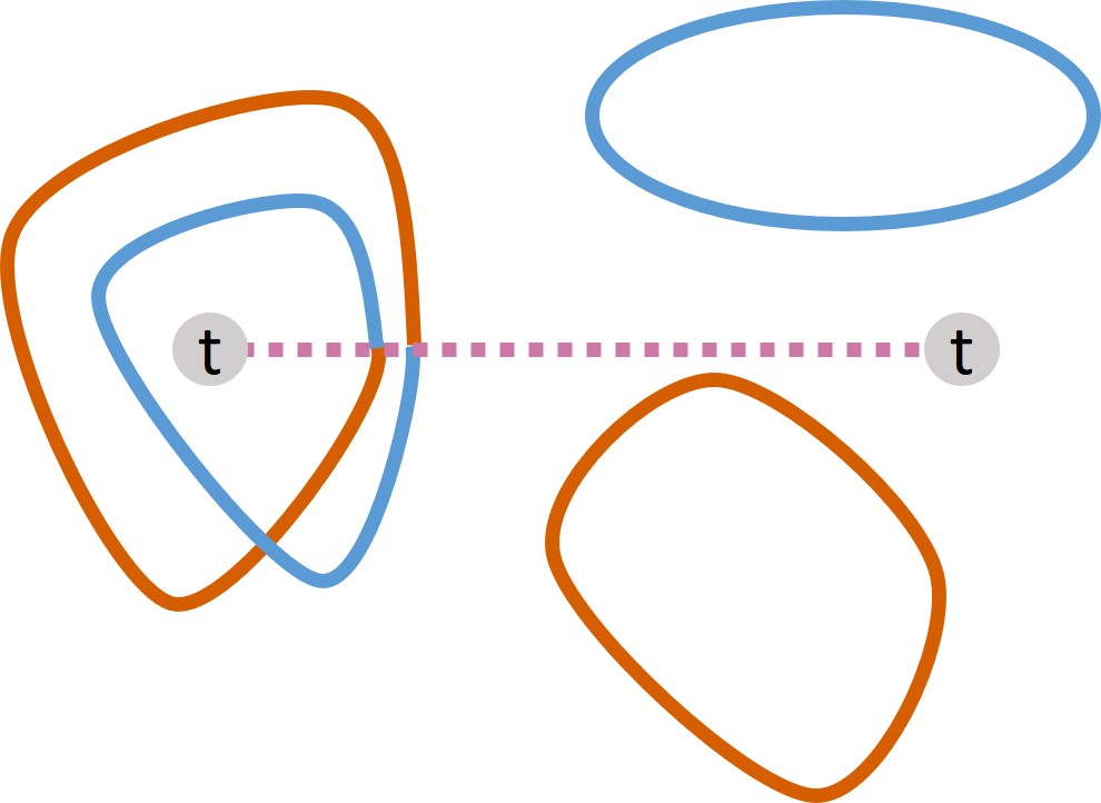

Gauging the SWAP symmetry means that the ground state is now also a condensate of closed branch cuts. Therefore, the ground state for the gauged model corresponds to a string-net condensate with three different colored strings - the strings in the original two layers of toric code (orange and blue), corresponding to the and spins, and the branch cut or “twist defect” strings (which we denote with purple), corresponding to the spins. Note that since the open twist defect strings corresponded to fluxes, the purple strings should be thought of as strings associated with the spins; thus here the presence or absence of a string corresponds to whether .
Given a particular configuration of the purple string condensate, we can still write down a string-net wavefunction for the orange and blue strings, but with the rule that whenever an orange or blue string crosses a purple string, it changes colors. An example string configuration is given in Fig. 4b. Note in particular that we may start with a configuration with no purple strings, create a closed purple string from the vacuum, wrap it all the way around the system (or bring it out to infinity if the system is on a plane), and then annihilate it. This implements a global SWAP operation; therefore, all ground states must be invariant under a global SWAP.
II.4 Ground state degeneracy
The string-net wave function picture is helpful to understand the ground state degeneracy of the gauged model on a torus by considering topologically nontrivial strings.
Before gauging, there are ground states labeled by the parity of the number of nontrivial strings winding around each handle of the torus in each layer.
After gauging, all states must be invariant under the global SWAP symmetry since the twist defects proliferate. Moreover, we are now allowed configurations where there are an odd number of twist defect strings (purple loops) wrapping around any handle of the torus. In the presence of an odd number of topologically nontrivial twist defect strings, the original strings acquire twisted boundary conditions; they must wind twice around the torus (since a layer 1 string becomes a layer 2 string and vice-versa after winding once around the torus), as shown in Fig. 5a. It is therefore most convenient to compute the ground state degeneracy by separately considering each topological sector for the purple strings (i.e. boundary conditions for the orange/blue strings), a task to which we now turn.

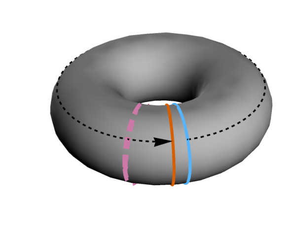
In the untwisted sector, we simply select the states of the ungauged theory which are symmetric under the global SWAP symmetry. It is straightforward to check that there are 10 such states.
In the sector with twisted boundary conditions around the handle only, a state can either have no string around the handle or have one string which winds twice around the handle, as in Fig. 5a. We also note that a string which winds around the (untwisted) handle in layer 1 can be translated all the way around the handle, in which case it becomes a string in layer 2, as in Fig. 5b. This also implies that the state with both colors of strings winding around the handle is equivalent to the state with no string around that handle. The superposition of strings winding around the handle is, however, topologically distinct and invariant under a global SWAP. In total, there are thus 4 states in this sector, and another 4 when the twist is instead only around the handle.
Finally, in the sector with twists around both handles of the torus, there are 4 states (each handle either has no string or a doubly-wound string).
In total, this means the ground state degeneracy is . This calculation can be straightforwardly extended to closed surfaces of any genus , which then allows extraction of the quantum dimensions of each of the topologically non-trivial quasi-particles through the formula
| (13) |
is the ground state subspace on a closed genus surface, , is the total quantum dimension, and is the quantum dimension of the quasiparticle labeled .
II.5 Excitations and string operators
The elementary excitations of the quantum double model are labeled by conjugacy classes and irreducible representations (irreps) of the centralizer , where the trivial conjugacy class corresponds to pure charges and the trivial irrep corresponds to pure fluxes. For labeling purposes, we give a convenient presentation of as . The nontrivial pure charges and pure fluxes in this topological order are listed in Table 1; all other anyons are dyons obtained from various fusions of the pure charges and pure fluxes. In total, there are topologically distinct quasiparticles.
| Label | Conjugacy Class | Irrep of | ||||||||||||||||
|---|---|---|---|---|---|---|---|---|---|---|---|---|---|---|---|---|---|---|
| 1 | 1 | 1 | 1 | 1 | ||||||||||||||
| 1 | 1 | 1 | 1 | 1 | ||||||||||||||
| 1 | 1 | 1 | ||||||||||||||||
| 2D irrep of | 2 | 1 | 1 | 1 | ||||||||||||||
| Trivial | 1 | 1 | 1 | 1 | 1 | |||||||||||||
| Trivial | 2 | 1 | 1 | 1 | ||||||||||||||
| Trivial | 2 | |||||||||||||||||
| Trivial | 2 | 1 | - |
Their properties can be understood systematically using the theoretical framework developed in Ref. Barkeshli et al. 2014. Here we briefly mention how to think of some of the quasiparticles. We can label the quasiparticles of the bilayer toric code model as , where are charge, flux, and fermion of the toric code. After gauging, the remaining quasiparticles are as follows. We have the invariant Abelian particles , , and , which retain their braiding and fusion properties even after gauging. The particles that are not invariant under the SWAP symmetry are grouped into orbits, , with , leading to the particles , , etc. Each of these particles is non-Abelian, with quantum dimension , and there are 6 such particles in total. Here the means that these particles can be roughly thought of as superpositions of the original particles, as seen in more detail in the next subsection.
In addition, we have the charge associated with the degrees of freedom, which is an Abelian particle labeled by . We also have a flux that corresponds to the twist defect after gauging, which also has quantum dimension . In total we can obtain twist defects and , for , which arise in the fusion outcomes of with the other particles. The particles thus correspond to , , and , with and , which gives a total of 22 particles. The particles are all Abelian, with quantum dimension , while , and are non-Abelian, with quantum dimension . In Table 1, we list how the pure charges and pure fluxes of the quantum double model can be related to this labeling.
In the next subsection, we will describe how these excitations can be understood in terms of gauging two copies of the toric code model, and we will explicitly construct the string operators that create the pure charge and pure flux excitations. The techniques used to construct the string operators in this model will carry over nicely to the fractonic case. In particular, we will develop an understanding of why some of the particles, such as , are non-Abelian with quantum dimension . We will explicitly see how the fusion rule
| (14) |
arises, both at the level of operators and also from understanding the string-net wave function picture.
Due to the structure of our model, there is no obvious mapping to a system whose degrees of freedom are elements of (the degrees of freedom do not quite match - there are two extra qubits per site), so we identify the excitations in the lattice model using the following intuition. Since conjugation by SWAP exchanges operators in the two layers, we will think of the Pauli operators (resp. ) as being related to the group element (resp. ), while SWAP is related to the group element . Since anticommutes both with anything odd under SWAP and with , we also think of as being related to the group element . This intuition can be confirmed by examining the fusion rules.
II.5.1 Wave function picture of excitations
All of the Abelian excitations have simple string operators, several of which arise from the original bilayer toric code. In particular, string operators in the ungauged model which create SWAP-invariant excitations are unaffected by the gauging procedure. For example, the Abelian charge should be identified with the bound state of excitations in both original toric code layers; it is straightforward to check that a string of operators creates this charge, just as it would in the ungauged model. In the string-net picture, this excitation just looks like a bound state of an open orange string and an open blue string, as in Fig. 6a.



Likewise, the flux is simply the bound state of excitations in both of the original toric code layers, and is created by a string of operators on the dual lattice. In our choice of string-net basis, whenever an odd number of blue and orange strings surround an excitation, the configuration enters the ground state superposition with a minus sign, as shown in Fig. 6b.
The other Abelian charges are also simple; a string of operators on the lattice of gauge qubits anticommutes with and commutes with everything else, so it should be identified as the gauge charge , which we denote as . In the string-net picture, configurations where an odd number of purple strings surround the excitation enter the ground state superposition with a minus sign, as in Fig. 6c. The other pure charge is simply the fusion of and .
The operators which create non-Abelian anyons are more interesting and quite instructive. Intuitively, the non-Abelian charge (which we shall dub ) can be thought of schematically as superposition of and from the ungauged model, since it arises from the symmetry orbit of the ungauged particles. It should therefore be constructed using and . In the subsequent section, we explicitly construct string operators for a variety of non-Abelian excitations and verify their fusion rules.
In the string-net picture, a pair of excitations (created from vacuum) are shown in Fig. 7a. The key point is that due to the presence of the proliferated branch cuts, the color of the string connecting the excitations is not definite, as whenever the string crosses a branch cut (purple string), it must change color. In this way, the excitation is, roughly speaking, a superposition of an (the end of an orange string) and an (the end of a blue string).


We next provide a pictorial understanding from the string-net wave function of why the non-Abelian excitations have the four fusion channels corresponding to the fusion rules in Eq. (14). Let us consider four excitations, corresponding to a pair of open strings, such that the overall fusion channel of all four is the identity. There is a remaining -fold topological degeneracy in this case: depending on the state, fusing the two open strings together leaves behind an open string associated with or . We can understand this four-fold degeneracy as follows.
Since no open branch cuts (open purple strings) are present, any string-net configuration can be deformed to a “reference” configuration where no branch cut are present at all. Such a reference configuration, which is unique up to a global SWAP, must have an even number of anyons associated with each layer to ensure that the configuration can be created from vacuum. It is immediately clear that there are four inequivalent (modulo a global SWAP) reference configurations consistent with these rules; they are shown as the first terms in Fig. 7b, along with several other terms in their string-net superpositions. There are therefore four states, each labeled by one of these inequivalent reference configurations, which can easily be checked to be orthogonal. This is exactly the desired topological degeneracy. To relate the degeneracy to fusion, consider the particular superpositions
| (15) | ||||
| (16) | ||||
| (17) | ||||
| (18) |
where normalization is ignored and the states are labeled on the right-hand side as they are in Fig. 7b, that is, O and B refer to the color (orange or blue) of the excitations in the reference configuration in clockwise order starting from the top left. We claim that the labeling on the left-hand side corresponds to the fusion channel for the top two and bottom two particles, that is,
| (19) |
where is an anyon label and the right-hand side is a fusion diagram.
To check that these fusion channels are correct, note that the two particles being fused have the same color in the reference configurations for and . As we allow the purple strings to fluctuate, the layer labels of the excitations change, but the color correlation remains. That is, every time that both excitations are surrounded by the same parity of purple strings, then the particles carry the same color label, and every time they are each surrounded by a different parity of purple strings, they carry different color labels. In particular, in every configuration in the superposition, moving these two excitations together (possibly crossing branch cuts along the way) will always lead to an meeting an from the same layer, so they can only fuse to the identity or . If instead we considered and , bringing the endpoints together always causes the s to carry opposite layers, meaning that only and are allowed fusion channels.

The presence or absence of a charge in a fusion product is measured with an operator which creates a pair of twist defects , braids them around the two excitations being fused, and re-annihilates said defects, leaving behind a closed branch cut. This operator’s support is far from the excitations, so it inserts this branch cut (modifying strings in the condensate as appropriate) without changing the color labels of the excitations as shown in Fig. 8. Deforming the resulting configuration to the reference configuration, also shown in Fig. 8 we find that when encloses the bottom two anyons. A more delicate examination shows that indeed as well. Therefore, has eigenvalue in the states and and eigenvalue in the states and , demonstrating that our claimed fusion outcomes are indeed correct.
II.5.2 Explicit non-Abelian string operators


Here we explicitly construct string operators for the non-Abelian excitations that correspond to pure charges and pure fluxes of the gauge theory. After constructing the operators, we then verify the resulting fusion rules of the non-Abelian quasiparticles.
We begin by considering the string operator for the excitation. As remarked in the previous section, this should be constructed using and . To ensure gauge invariance, we should start with a string of operators, where disjoint pairs of operators are connected pairwise by a string of operators. Such operators commute with and everywhere, but not with any ; this is a problem because the fact that the quasiparticles are deconfined requires that our string commute with all the away from the end of the string. To ensure that this occurs, we use equations like the one in Fig. 9a, which arise directly from the commutation relations Eq. (3). In particular, commuting a string of operators permutes the various summands in at the cost of interchanging on the edges touching site (and dressing with operators). Superposing over all operators obtained by these interchanges, as in Fig. 9b, will therefore produce a string operator which commutes with the Hamiltonian everywhere except at its endpoints; the resulting excitation is the particle.
If the local unitary acts on the end of the string operator, which interchanges and on that link only, we obtain a new string operator which no longer commutes with on the last link of the string, but still commutes with all other terms along the length of the string. This new operator therefore also creates at its endpoints. There are four such operators, specified by the four choices of sign at the endpoints of the operator in Fig. 9b, which we call in accordance with Fig. 9b. The two signs refer to the left and right endpoints of the string respectively.
The string-net picture also gives us another way to understand the structure of the operator . Suppose that we consider configurations where the left end of the string in Fig. 7a is orange, that is, we act with where the lower index indicates that it is the first link in the string. Then to continue the string operator, we should act with if an odd number of branch cuts pass between links 1 and 2, and act with if an even number do. This is expressed by acting next with the operator
| (20) |
where is the product of on a string of gauge spins connecting links 1 and 2, because measures the parity of the number of branch cuts passing between links 1 and 2. Continuing, we obtain a string operator
| (21) |
The same thing can be done starting from a blue link, i.e. beginning with , which, following the same logic, leads to a string operator
| (22) |
Adding these together (to obtain a globally SWAP-invariant operator), one can check that
| (23) |
The same idea of choosing a particular gauge-invariant string operator and then interchanging local operators to ensure that the string has no tension can be used to find (largely by inspection) the rest of the string operators in the theory. Below we formalize this structure and give a list of the string operators for all the pure charges and pure fluxes in the theory. (Dyon string operators can of course be constructed by taking products of the charge and flux operators.)
We specify the string operators as a superposition of products of local operators. For an Abelian anyon, there will only be one term in the superposition, whereas for a non-Abelian anyon, the superposition will contain terms, where is the length of the string. As we will explain shortly, the strings all have a common structure which is specified by six local operators. Their locations are shown in Fig. 10. Two, which we shall call and , live on the square lattice links along the length of the string. Two, which we shall call and , live on the square lattice links jutting out from the string. The last two, which we shall call and , live on the links. The choice of whether , , and or , , and appears at various positions on the string will specify the different terms in the superposition.
A convenient way to explain the structure of the operators is as follows. To form our superposition of local operators, start from a “reference” operator where the body of the string consists entirely of , , and operators, as in Fig. 10a. For non-Abelian quasiparticles, the operators with the signs should be chosen to commute with all gauge generators and the operators with the signs are chosen to anticommute with any with overlapping support. This ensures that the reference operator is gauge-invariant.


Next, for a length- string, construct string operators as follows. Given the reference string for a pure charge (resp. flux) excitation, proceed down the string from site to site (resp. plaquette to plaquette). At each site (resp. plaquette), choose whether or not to interchange ,, and on the links surrounding that site (resp. within that plaquette). After making such a choice on every site (resp. plaquette), we have obtained a new product of local operators; our desired string operator, which we denote (where labels the anyon type and the signs indicate whether is chosen on the left and right ends of the string, respectively) is simply the superposition over all such choices. An example term is shown in Fig. 10b for the pure charge excitations and Fig. 10c for the pure flux excitations. Obviously, if , and , all of these terms are the same and there is only one term in the superposition; such a string operator will create Abelian anyons.
Given this structure, the ,, and operators are chosen such that this superposition procedure causes to commute with the Hamiltonian everywhere except at its ends. In the non-Abelian case, this is done with equations similar to the one in Fig. 9a that we used for the anyon.
The full set of operators, along with their identifications, are listed in Table 1. Note in particular that we have an explicit form for the string operator for the twist defect .
The string operator algebra can also be used to obtain (partial) information about the fusion rules of the theory. Because the string operators, when acting on the ground state, create excitations from the vacuum, every string operator obviously creates excitations which fuse to the vacuum sector. Furthermore, given two string operators and supported on the same region which create the anyons and respectively at their ends, their product must create fusion products at each endpoint (we make no distinction between particles and antiparticles here because in topological order, all particles are their own antiparticles). The string operator algebra should thus contain operators such that
| (24) |
for any , where are fusion multiplicities. Note that if is a local operator, and defining
| (25) |
then Eq. (24) still holds with replaced by . However, a product like need not obey the same equation, so only certain elements of the string operator algebra produce the full list of fusion outcomes.
We defer an exhaustive enumeration of the string operator algebra to Appendix B and presently consider some representative examples to demonstrate the fusion rules. Consider first fusing any of the Abelian charges with themselves. Their string operators square to the identity, which means that, as expected, these charges are Abelian and are their own antiparticles.
Next, consider fusing the charge with the non-Abelian charge. Since , multiplying the string operator in Fig. 9b by the string operator which creates the excitations produces the same string operator for the non-Abelian charge up to a possible minus sign (since the number of operators has the same parity for every term in the sum). Therefore, these charges fuse to the non-Abelian charge, verifying the fusion rule
| (26) |
This is also easy to see in the string-net wave function picture: Fusing an open string of both colors onto the non-Abelian string clearly just permutes the terms in the ground state superposition for the non-Abelian string (e.g. it switches the terms with a purely orange string and a purely blue string), thus giving us back the same picture.
Finally, consider fusing the non-Abelian charge with itself. Using the operator definitions in Fig. 9b, a straightforward but tedious calculation shows that, up to normalization,
| (27) | ||||
| (28) |
where the tensor products are over the full length of the original string operator. The second line, where we identify these operators with string operators for Abelian charges, follows by inspection. That is, all of the Abelian charges are possible fusion outcomes of two non-Abelian charges. By counting the quantum dimension, one can check that this exhausts all possible fusion outcomes. The operator algebra for the individual is listed in the Appendix.
III Gauged Bilayer X-Cube
The X-cube model has been discussed elsewhere in considerable detail Castelnovo et al. 2010; Vijay et al. 2016. We give a brief overview of its properties in Appendix C. In this section, we construct the gauged bilayer X-Cube model, provide a cage-net picture for the ground state wavefunctions, and sketch the calculation of the ground state degeneracy on a 3-torus, relegating technical details of the calculation to Appendix E.
III.1 Construction of the model

The procedure is analogous to the bilayer toric code case. The ungauged model consists of two layers of spins on the links of a cubic lattice with two copies of the X-Cube Hamiltonian:
| (29) | ||||
| (30) |
with and the usual star and cube operators shown in Fig. 11. Here labels a site, labels the orientation of the star operators, and labels elementary cubes. For each term in the ungauged model, we can rewrite the sum of the two layers’ terms as a sum of products of SWAP-even and SWAP-odd operators; for example,
| (31) |
where . As before, we have suppressed the explicit position index on the operators. To gauge the symmetry, we add gauge qubits connecting nearest neighbor links. This corresponds to adding an octahedral “cage” of gauge qubits surrounding each site, as in Fig. 12a. Next, we define a gauge symmetry generator
| (32) |
where the act on the eight gauge qubits which neighbor an edge of the original cubic lattice; this operator is shown in Fig. 12b. We also define gauge flux operators
| (33) | ||||
| (34) |
Here acts on each face of the octahedron of gauge spins surrounding each site and acts on the four spins within a face of the cubic lattice, as shown in Fig. 12d.
We now modify the Hamiltonian so that the model is invariant under the gauge symmetry generated by . This invariance is obtained by putting operators into the Hamiltonian terms such that every term has an odd number of operators acting on the qubits which surround it. This can always be achieved by choosing disjoint pairs of operators and connecting them with a path of operators. Some examples of the 2048 terms are shown in Fig. 12c.


The gauged Hamiltonian is
| (35) |
where is the sum of the eight gauged star terms for each orientation of the star and is the sum of the 2048 gauged cube terms.
All of the algebraic computations for the gauged bilayer toric code model carry through for the gauged bilayer X-Cube model. That is, , , and square to 1, while the and operators square to . Likewise, , , , , and all mutually commute.
III.2 Wavefunction picture of ground states
The basic building blocks of our wavefunction picture for the ground states is the cage-net picture for a single layer of the X-cube modelPrem et al. 2018b, which we now briefly review.
Configurations where on a link are drawn with no string, whereas is represented by the presence of a string on a link. In the ungauged model, strings are colored to represent their layers (orange for layer 1, blue for layer 2) and both colors can live on the same link. A configuration with no strings is an eigenstate of all the operators with eigenvalue , but not of the operators. Requiring that amounts to superposing over all configurations of closed “cages” of strings of each color, where an elementary (i.e. minimal size) “cage” is the wireframe outlining a unit cell cube. An example configuration in a ground state superposition for the ungauged bilayer model is shown in Fig. 13a.


Distinct ground states on the 3-torus are labeled by the presence or absence of strings which wrap all the way around each handle of the torus. Not all such strings are independent; we will discuss the constraints between them in Sec. III.3.
The system now supports extrinsic co-dimension 1 membrane defects, whose boundary is a twist defect string. The membrane acts as a branch sheet, such that excitations that cross it go from one layer to the other. That is, any leg of a cage which passes through a branch membrane associated with the twist defect must change colors. Hence any cage which links nontrivially with the twist defect must wrap the defect twice, as shown in Fig. 13b.
Upon gauging, the ground state now also consists of superpositions of all possible closed branch membranes. We therefore obtain two colors of cage-net condensates and a conventional condensate of closed membranes, generally shown in purple, which correspond to the spins. The wavefunction for the membrane sector is the same as in conventional (3+1)D topological order. However, the cage-nets are subjected to the rule that if a leg of a cage crosses a membrane, it changes colors. An example configuration in the ground state superposition is shown in Fig. 13c.
As usual, a closed branch membrane can be nucleated from the vacuum, wrapped all the way around the system, and annihilated, which implements a global SWAP. Hence all ground states should be invariant under a global SWAP.
III.3 Ground state degeneracy on 3-torus
The detailed calculation of the GSD on an 3-torus is quite involved, requiring considerable constraint counting. The full details of this calculation are relegated to Appendix E; here we present an outline of the calculation and its result.
In a copy of the ungauged X-Cube model, ground states are labeled by the eigenvalues of Wilson loop operators which physically correspond to creating a particle-anti-particle pair for a particle constrained to move in one dimension, winding one around the torus, and then annihilating the particles. These Wilson loops are products of operators. Since the quasiparticles involved are one-dimensional, these Wilson loops are rigid, naively leading to distinct string operators with . However, there is a constraint; the product of any four Wilson loop operators which live on the edges of a rectangular prism, as shown in Fig. 14a, is equal to the identity in the ground state (in the wavefunction picture, any four such strings can disappear). This follows from the energetic constraint that the product of over the edges of a cube is equal to . Therefore, in the cage-net wavefunction picture, we may freely create or delete such a set of strings.
It is straightforward to show that a basis for the independent -oriented Wilson loop operators is all such strings which are at and all such strings at for a fixed choice of , as shown in Fig. 14b. This leads to independent -oriented Wilson loop operators. Including also the independent and oriented Wilson loop operators then leads to a total of
| (36) |
Wilson loops in each copy of the X-Cube model. In the wavefunction picture, we represent a eigenvalue as the absence of a Wilson loop and a eigenvalue as the presence of a Wilson loop. Two copies of the X-cube model thus have ground states in total.


For brevity, we call a particular string position and orientation its “type” and refer to the X-Cube layer separately.
Upon gauging the bilayer model, we first restrict to configurations of the ungauged model where all layer-twist membranes are topologically trivial. The different states may then be labeled by “reference configurations” where no topologically trivial membranes or strings are present, as the other states in the superposition are obtained by allowing local fluctuations of membranes and cages. However, we must project to ground states of the ungauged model which are invariant under a global SWAP operation.
For each independent string type, if a configuration contains either no strings or both layers’ strings, then the configuration is obviously symmetric under SWAP; there are such configurations. Given any of the other string configurations , a global SWAP acts nontrivially, so only the symmetric combination of and invariant. Hence the total number of states in the untwisted sector is
| (37) |
However, due to the proliferated layer-twist defects, additional ground states are available. In particular, the twist defects, which are created by flexible membrane operators, can extend all the way around the torus without costing energy. In a ground state on the 3-torus there are three independent possible twist defects corresponding to stretching the layer-twist membrane around the and , and , and and handles, an example of which is shown in Fig. 15a.
These layer-twist defects are branch membranes for the strings and substantially change the ground states because a Wilson loop which passes through a layer-twist defect changes layers. For example, in the presence of a twist defect in the plane, a -oriented string must wrap around the torus twice in order to close, as shown in Fig. 15a. Furthermore, the set of constraints on strings which do not pass through a twist defect also changes. The constraint that four strings on the edges of a prism are equal to the identity (see Fig. 14a) is modified in the presence of the twist defect to the one shown in Fig. 15b. Using these constraints, certain pairs of strings can be translated in certain directions, e.g. two -oriented strings at the same position can be translated in the direction, as shown in Fig. 15c. If the strings are translated all the way around a handle of the torus, in the presence of an appropriate twist defect they change layers, as shown in Fig. 15c. This leads to additional constraints between the Wilson loops in different layers. This is similar to the gauged bilayer toric code; in that case, single strings around the untwisted handle can swap layers by being translated around the twisted handle. It is the same situation here, except only certain pairs of strings can be translated around the twisted handle.


IV Excitations of the Gauged Bilayer X-Cube Model
In this section, we discuss at length the excitations of the gauged bilayer X-Cube model Eq. (35). In particular, we show how the string operators for the non-Abelian excitations are constructed. We then compute the degeneracy associated to the string-like twist defects and discuss some examples of bulk braiding analogs associated to the non-Abelian fractons.
Similarly to the toric code case, the (ungauged) bilayer X-cube model has excitations which can be labeled as where and bound states of those particles. (See Appendix C for a review of the excitations of a single layer of the X-cube model using the labeling of Ref. Bulmash and Iadecola 2019.) Here , for , is a one-dimensional particle which moves only in the th direction, associated with exciting two star operators on the same site, and is the fracton associated with an excited cube operator. Note that we are suppressing position indices since the true superselection sectors depend in a complicated way on the positions of various excitations. We will also occasionally refer to a two-dimensional particle called , where are the directions of mobility; this excitation is a bound state of two face-sharing cube excitations separated in the direction where .
Upon gauging, any SWAP-invariant particle remains Abelian; in our case, these are , , , and bound states thereof. The non-invariant particles are grouped into orbits and , which are non-Abelian. As in the toric code case, means a rough identification of the particle type with superpositions of the original particles. The non-Abelian quasiparticles have quantum dimension 2. Again, there is a charge associated with the degrees of freedom, which we shall call and will turn out to be fully mobile. Upon gauging, the string-like twist defect becomes a flexible string-like excitation , which can bind various point excitations.
The pure charge excitations of the gauged model can be identified with representations of in the same way as in the gauged bilayer toric code case, but it is not clear that it is particularly meaningful or useful to describe the purely magnetic excitations in terms of conjugacy classes. In general, monopoles (fractons) and fluxes are created by membrane operators. The nontrivial simple excitations are listed in Table 2.
| Label | Excitation | Mobility | ||||
|---|---|---|---|---|---|---|
| Point charge | 3D | 1 | ||||
| Point charge | 1D | 1 | ||||
| Point charge | 1D | 1 | ||||
| Point charge 2D irrep of | 1D | 2 | ||||
| Abelian monopole | Fracton | 1 | ||||
| Non-Abelian monopole | Fracton | 2 | ||||
| Flux (twist) string | Flexible string excitation |
IV.1 Quasiparticle excitations
IV.1.1 Abelian excitations
The bound states of excitations in both layers are Abelian and created in the same way as in the ungauged model; for example, a (rigid) string of operators creates the one-dimensional particle associated to the irrep , which are, in the cage-net picture, the endpoints of a string of both colors, as in Fig. 16a.


A rectangular membrane of operators creates four Abelian fractons . In the cage-net picture, this corresponds to having a minus sign in the ground state superposition whenever an odd number of cages surround the location of the fracton, as shown in Fig. 16b.
Similarly, the charge is created by a string of operators acting on gauge qubits. Since this string commutes with , , , and and anticommutes with , is easily checked to be fully mobile. This is not surprising since each spin appears in exactly two operators. In the wavefunction picture, this excitation corresponds to minus signs in the ground state superposition whenever a branch membrane surrounds the excitation in question, as in Fig. 16c.
IV.1.2 Non-Abelian fractons - cage-net picture
We begin with a cage-net picture of the wave function in the presence of the non-Abelian fracton . We will find the remarkable result that the degeneracy in the presence of many fractons depends on their relative positions. We further use the wave function picture to understand how this degeneracy can be understood in terms of fusion properties of the fractons. Subsequently we demonstrate certain fusion rules explicitly by studying the quasiparticle operator algebra.
The excitations are created in sets of four at the corners of rectangular membrane operators. The local cage-net configurations near a single fracton are shown in Fig. 17. In particular, we start with a “reference” configuration where the fracton excitation is labeled with a definite layer index (color, in our pictures). When is surrounded by an odd number of cages of its own color (in the absence of any branch membranes), the term in the superposition switches sign, as in the first two terms of Fig. 17. The excitation also switches colors when surrounded by a branch membrane. Note that since branch membranes do not preserve the color of cages, the configuration where an orange cage surrounds both a blue fracton and a branch membrane has the same sign as the configuration where an orange cage surrounds an orange fracton, as in the configurations in Fig. 17. This is because these two configurations are related by deforming the branch membrane through the fracton in question, which switches the color of the fracton without introducing an additional minus sign.

Let us now consider the degeneracy associated with the excitations. It is important to realize that, just as in the ungauged model, there is a constraint at the level of the Hilbert space: in any reference configuration, the number of fractons of each color in every plane perpendicular to a coordinate axis is even. This follows from the operator identity
| (39) |
That is, a cage of any fixed color which encloses an entire plane is exactly the same as no cage at all.
Therefore, the number of ground states for a given spatial configuration of fractons is given by the number of ways of assigning layer labels to each fracton (modulo a global SWAP), subject to the above constraint. The requirement of satisfying the above constraints leads to a highly non-trivial position-dependence of the degeneracy, as we see explicitly in the following examples.
In the presence of four excitations at the corners of a rectangle, there is only one allowed reference configuration up to a global SWAP (in which all excitations have the same color), so there is only one state.
Consider next eight excitations on the corners of a cube (or a rectangular prism). Then it is easy to check that, up to a global SWAP, there are eight possible reference configurations consistent with the aforementioned identity and which are inequivalent under proliferation of cage-nets. One example reference configuration is given in Fig. 18a along with a few terms in its cage-net superposition. Distinct configurations are locally indistinguishable because the layer index for an individual fracton is not a good quantum number, so there are eight degenerate states associated with these fractons. This is a general rule; the number of distinct reference configurations up to global SWAPs equals the degeneracy. Generalizing this, in the presence of fractons created in quartets of four fractons in the geometry shown in Fig. 18b, simple combinatorial arguments show that the number of inequivalent reference configurations and therefore the number of locally indistinguishable degenerate states is .


When instead eight fractons are placed in the geometry shown in Fig. 18c , there are only four allowed reference configurations, and in the geometry shown in Fig. 18d, there are only two allowed reference configurations. Hence the number of states associated with eight excitations depends strongly on their relative positions. This position-dependence of the degeneracy is consistent with the fact that in a fusion category description of fractons, their superselection sector of depends on their positionPai and Hermele 2019.
The locally indistinguishable, degenerate states arising from the fractons can be labeled in terms of fusion properties of the fractons, as we now describe. We note that a complete theory of fusion rules is complicated by the fact that fractons at different spatial positions are in distinct superselection sectors, and a complete theory of fusion should properly take this into account. As such, here our discussion of the fusion properties is limited to a description of how to label the different states in terms of the eigenvalues of certain extended cage or membrane operators that can measure certain topological charges associated with a given region. We leave a more comprehensive theory of fusion rules in such non-Abelian fracton models as an open problem.
Just as in the gauged bilayer toric code case, the layer label for each fracton is not definite, but the layer parity of any pair of fractons in a cage-net configuration depends only on the corresponding layer parity in the relevant reference configuration and the number of branch membranes surrounding those two fractons. Therefore, an operator which creates a cage of either color surrounding two excitations has a definite eigenvalue of in each of these eight reference configurations. We interpret these two possible eigenvalues as assigning to the given region an even or odd topological charge of the Abelian fracton .
One can also assign a charge to certain regions, which can be measured by the eigenvalue of a membrane operator . However, not every region can be assigned such a definite topological charge. The desired operator creates a flux string, moves it around the region in question, and attempts to re-annihilates the string. Analogous to the case of in the gauged bilayer toric code case, does not change the color of fractons inside the region it is associated with, since its support is far from those excitations; nevertheless, it leaves behind in the wave function a branch membrane. Suppose first that surrounds two excitations. After deforming back to the reference configuration, two fractons switch colors, which violates the constraint that all planes perpendicular to coordinate axes contain an even number of fractons of each color. Therefore, such a process is actually not possible. This process is depicted in Fig. 19a. Stated differently, must take us out of the degenerate manifold of states to a different excited state rather than re-annihilating the string. A similar phenomenon occurs in, for example, the (2+1)D Ising topological order, where a non-Abelian loop cannot enclose a single non-Abelian particle, because of the difference in fusion channels between the initial and final state.
Nevertheless, there exist choices of four such that applying a membrane that surrounds them, as in Fig. 19b, leads to a configuration which obeys the constraints. This means that a definite charge is only associated to certain choices of four well-separated excitations, not two.


Therefore, any pair of fractons can be assigned a definite parity, but only certain sets of four fractons can have a definite parity. In particular, certain superpositions of the reference configurations, such as the one shown in Fig. 19c, are cage-net states with definite (resp. ) parity for all pairs (resp. quartets) of fractons in the same -plane. One can also check that this fusion information is sufficient to distinguish all of the eight degenerate states.
Let us now turn to a discussion of quantum dimension. In conventional topological order, the quantum dimension of a particle of type can be defined by considering the degeneracy in the presence of particles of type , which scales as . However since in the present context the degeneracy in the presence of fractons depends sensitively on their relative position, the definition of the quantum dimension of is more subtle.
In fact, because the superselection sector of fractons depends on their positions, the geometries considered above actually involve fusion of excitations in different superselection sectors. Thus, to define a quantum dimension for , we wish to create a set of excitations which are all in the same superselection sector. This can be done by considering a set of fractons in the geometry shown in Fig. 18e. In this geometry, there is a membrane operator which turns the excitations in any one grey box into the excitations in any other grey box - in particular, each one can independently be turned into a copy of the grey box with a single inside. This means that each grey box should be thought of as living in the same superselection sector as the single . In this geometry, for each reference configuration, all fractons in each grey box must be in the same layer in order to obey the global constraints. Simple counting shows that up to a global SWAP, there are degenerate states in this geometry, where is the number of grey boxes (provided is even, or no states are allowed at all). Therefore we find that the quantum dimension
| (40) |
IV.1.3 Non-Abelian fractons - explicit operators
With the cage-net understanding in hand, we now explicitly construct the operators that create the non-Abelian fractons . Following the intuition from the gauged bilayer toric code, we expect that we should build a (gauge-invariant) membrane operator from and since these commute with . However, the membrane should commute with the Hamiltonian everywhere except at its corners. Commuting past a membrane of operators will permute the various summands of at the cost of interchanging with and dressing with some operators, as in Fig. 20a. Therefore, superposing over all such interchanges will produce the desired membrane operator. Some examples have the form shown in Figs. 20b and 20c; these operators create four fractons .


There are in fact sixteen different such operators; they can be obtained from the one shown in Fig. 20b by choosing any subset of the corners of the membrane and exchanging and in every term of the sum at the chosen corners. These operators differ from each other by the local action of at the corners. For future reference, we call these operators , where the signs refer to whether there is an or an at each corner in the term in the sum with no operators, as labeled in Fig. 20.
As a suggestive calculation for the fusion channels, we explicitly compute products of the membrane operators. For the full operator algebra, see Appendix D.
Let
| (41) |
This is a particular choice of membrane operator which creates four fractons at its corners. Applying to the ground state creates two fractons at each corner of the membrane. We can fuse the two fractons at each corner into simple excitations; this amounts to re-expressing as a sum of operators creating simple excitations at each corner of the membrane. A tedious computation similar to the one done for the bilayer toric code shows that
| (42) |
where label distinct corners of the membrane and “stringij” means any string connecting the corners and . In particular, we can identify this as a sum of the identity, the operator creating four fractons, an operator creating any even number of charges , and the bound states . (Note that the string operators for can fluctuate between connecting any choice of pairs of excitations.)
That is, there are four distinct outcomes for the fusion at each corner of the membrane: , , , and , which can be chosen independently provided the total fusion is the identity. This naively seems to “overcount” compared to the cage-net picture, where a definite parity of is only well-defined for a set of four fractons rather than a pair. However, in the present calculation, the fractons being fused are at the same location in space, so their fusion outcome can be distinguished by local operators (i.e. by arbitrarily small membrane / cage operators). It is not necessarily true that these locally distinguishable states all correspond to distinct degenerate states when the fractons are widely separated, especially given the geometry dependence of the non-Abelian degeneracy. However, when widely separated fractons are brought close together, the final fusion channels will of course be consistent with the fusion when the particles are well-separated.
IV.1.4 General operator structure
We now exhibit the operators which create the full set of simple excitations in this model, deferring the full enumeration of their algebra to Appendix D.
There are four types of operators which we need to consider: flexible string operators, which create charges (discussed previously), rigid string operators, which create excitations in the sector, rigid membrane operators, which create fractons, and flexible membrane operators, which create twist defect strings. We handle each one in turn, starting with string operators.
The structure of rigid string operators in the gauged bilayer X-cube model is the same as the string operators for pure charge excitations in the (2+1)D gauged bilayer toric code case (see Appendix B); the only difference is that the strings are rigid. In particular, the string operators are constructed from a set of local operators , although it so happens that in this sector the are the identity. We will therefore ignore the for the rest of the discussion.
As before, we start from a reference string as in Fig. 10a with only and appearing in the string except at its ends; either may be chosen at the end, which correspond to local degrees of freedom of the quasiparticles, that is, this choice can be modified via the action of a local operator. Next, for every lattice site along the length of the string, we choose whether to flip for all links surrounding that site, as in Fig. 10b, obtaining a new operator. We then superpose over all such choices.
The quasiparticle types are: Abelian one-dimensional (1D) quasiparticles , where labels the direction of mobility, Abelian 1D quasiparticles , and non-Abelian 1D quasiparticles . A specification of their string operators is listed in Table 3.
| Label | Excitation type | |||||||||
|---|---|---|---|---|---|---|---|---|---|---|
| mobile boson | 1 | 1 | ||||||||
| Abelian 1D particle | 1 | 1 | ||||||||
| Abelian 1D particle | ||||||||||
| non-Abelian 1D particle | 1 |
We next turn to the rigid membrane operators, which create fractons, and describe them in a more systematic framework. The basic excitations in this sector are and , which are Abelian, and , which is non-Abelian.
We again take a reference operator and superpose flipped versions of that reference operator, as described in previous examples. The distinction is that this time, all of the local operators which border an elementary cube of the cubic lattice are affected by the flipping procedure. We again define , , and operators, which live now on the links in the plane of the membrane (both on top and on the bottom of the membrane), links puncturing the membrane, and on half of the links within the membrane, respectively, as in Fig. 21. In the fracton sector, the are always 1, so we ignore them in what follows, but we have defined the for the purposes of discussing twist strings later.

The reference operators are defined to have and everywhere on the membrane, except we allow either or at the corners of the membrane. This leads to sixteen possible operators specified by four choices of in the reference configuration; these sixteen operators will differ by the action of local operators at the corners of the membrane, that is, they specify purely local degrees of freedom of the fractons.
Now form more membrane operators by, for each face within the membrane, choosing whether or not to exchange on all the operators which touch that face. Finally, superpose over all the membrane operators we have formed from a given reference configuration.
The operator choices for the fractons and twist strings are given in Table 4. Some example terms in the superposition for the excitation are given in Figs. 20b and 20c.
| Label | Excitation type | |||||||||||||
|---|---|---|---|---|---|---|---|---|---|---|---|---|---|---|
| Abelian fracton | 1 | 1 | 1 | 1 | ||||||||||
| non-Abelian fracton | 1 | 1 | 1 | |||||||||||
| non-Abelian twist string | 1 |
Finally, the flexible membrane operators which create twist strings are constructed similarly to the membranes which create fractons, but with some important differences. First, rather than only choosing between at the corners of the membrane in the reference configuration, we may choose or anywhere on the boundary of the membrane operator. This is reasonable because the string excitation it creates may generally have a local degree of freedom at each point on the string. Second, instead of interchanging on all operators touching a face within the membrane, we interchange on all operators touching cubes within the membrane. Each cube affects eight s, four s, and eight s. Otherwise, the construction is the same. The appropriate operators for are listed in Table 4.
IV.2 String excitations and geometry-dependent degeneracy
In this subsection, we show that a string excitation is associated with a topological degeneracy that scales as where is the linear extent of that excitation in the direction. This is qualitatively different from conventional topological order in (3+1)D, where non-Abelian string defects carry a degeneracy that is independent of their size and shape. We demonstrate this first by considering an extrinsic twist defect in the ungauged model. After gauging, the extrinsic twist defect becomes one of the string excitations. We will first compute the degeneracy in the ungauged case, with the degeneracy after gauging following straightforwardly.
For simplicity, we consider our system to be a large but finite-size cube. We choose boundary conditions where the one-dimensional “” particles (violations of star terms in ) in both layers of the original X-cube model are condensed at the boundary (“rough” boundary conditions). It is straightforward to check (in the wavefunction picture) that in the absence of excitations, the ground state is unique because there are no topologically nontrivial strings in the sector (associated to violations of the cube terms in ). Hence, any degeneracy will be associated with excitations. The exact degeneracy will depend on boundary conditions, as it does for conventional topological order, but the quantum dimension is independent of the boundary conditions.
Consider first two decoupled copies of the X-cube model with an extrinsic twist defect string inserted, as in Fig. 22a. We presently set notation. Call violations of the terms (see Eq. (30)) as , where labels a layer and labels the direction of motion of these one-dimensional particles. Bound states of excitations of two face-sharing terms are two-dimensional particles, which we call , where means that this excitation is mobile in the -plane.
Note that quasiparticles have closed Wilson loop operators (closed strings of ) associated to creating a pair of quasiparticles, moving them in a loop, and re-annihilating them. Because is mobile only in the -plane, Wilson loops can be deformed in the -plane but not out of that plane. On the other hand, can form Wilson lines by creating a pair in the bulk, moving them to the boundary, and annihilating them. These Wilson lines are completely rigid because is only mobile in one dimension.


With the notation set, consider a closed Wilson loop for an particle which surrounds the defect string, as shown in Fig. 22a. This Wilson loop cannot be deformed to the identity because, due to the subdimensional nature of the excitations, the Wilson loop cannot be deformed out of the -plane. This is in contrast with conventional topological order, where, thanks to the full mobility of the particles, Wilson loops can be deformed arbitrarily. Such a Wilson loop anticommutes with any Wilson line which passes through the defect in the same -plane because the particle changes layers when it passes through the defect, as shown in Fig. 22a. There are therefore nontrivial Wilson loops in the presence of the defect (the counts layers). The same holds for Wilson loops for particles, so in total there are nontrivial Wilson loops.
However, not all of these Wilson loops address independent states; we must count independent Wilson lines as well. The constraint discussed earlier also applies to Wilson lines which pass through the defect - the product of any four Wilson lines at the corners of a rectangle must equal the identity. Therefore, there are only independent Wilson lines, as shown in Fig. 22b, and each of them anticommutes with (at least) one Wilson line. The degeneracy in the presence of the defect is therefore .
We now wish to examine what happens when the loop bends in the -direction as well, say in the -plane as in Fig. 22c. It is easy to see that independent Wilson lines pass through the defect. Likewise, there are additional Wilson lines that surround the defect, which each anticommute with an Wilson line. However, there is no additional Wilson loop which anticommutes with the other Wilson lines; those are already being “used” as logical operators which anticommute with the Wilson lines. We therefore get an additional degeneracy of only , leading to a total degeneracy of .


Next, we briefly discuss what happens in the presence of multiple defect strings. If the strings are not linked, it is not too difficult to see that an independent set of Wilson lines for each string can be constructed, on the right side of Figs. 23a and 23b. There is also an independent set of “Wilson lines” for each string; in particular, by using the fact that can split into an and an , the particles can “go around” a string defect in the way shown on the left side of Figs. 23a and 23b. Therefore, the degeneracies associated to each string are independent.
If the strings are linked, the degeneracies are still independent; this time, the fact that the Wilson lines are distinct follows straightforwardly from the geometry, as in the left sides of Figs. 23c and 23d, and the independent Wilson lines are obtained by wrapping around either one or both strings, as shown on the right sides of Figs. 23c and 23d. Therefore, since each defect contributes independently to the degeneracy regardless of the relative configuration of the strings, the quantum dimension of the string defect is really .
Finally, we promote our understanding of the ungauged model to the degeneracy in the gauged model. Before gauging, the number of degenerate states associated with a string excitation scales as . Because the degeneracy is associated with the twist defect and not with the boundary conditions (although the boundary conditions can affect the total degeneracy), after gauging, all that happens is that we restrict to the states which are symmetric under a global SWAP. Following similar arguments used for the ground state degeneracy on the torus in Sec. III.3, there are states associated with the string. The quantum dimension is therefore in the gauged model.
IV.3 Non-Abelian braiding analog for subdimensional particles
Although a full theory of braiding for subdimensional particles has not yet been developed, we can demonstrate that our model possesses an analog of non-Abelian braiding of subdimensional particles.


Let be a ground state, and consider the state , where is a membrane in the -plane centered at and is large. Physically, this corresponds to creating eight excitations, one at each corner of a rectangular prism. One can check from the operator algebra (see Appendix D) that . Next, let be a closed “cage” operator for the particles; physically, we create from vacuum a triple of , , and at each corner of a wireframe cube, then move the particles and annihilate them pairwise. Explicitly, is shown in Fig. 24a and is simply an “enlarged” version of . One can check that , and therefore (assuming that the linear size of is small compared to the system size). One can also check explicitly that if is positioned so that it surrounds exactly two fractons, as shown in Fig. 24b, then
| (43) |
Here the position indices on are suppressed for legibility. It immediately follows that
| (44) |
so and have the same type of excitations at the same locations. Hence (again using the operator algebra in Appendix D)
| (45) | ||||
| (46) |
It is likewise straightforward to check that has nonzero norm. Therefore, performs a non-trivial unitary transformation on the set of degenerate states associated with the eight excitations created by , such that and are orthogonal. This is precisely a consequence of an analog of non-Abelian braiding for subdimensional excitations.
V Gauged Bilayer Haah’s Code
Our primary interest in gauging the layer-swap symmetry of Haah’s code will be to show that there are non-Abelian fractal-type fractons in the model. (We call quasiparticles created at the corners of operators with fractal support, e.g. the quasiparticles in Haah’s code, “fractal-type”. Our model does not fall cleanly into the “type-I”/“type-II” dichotomy of Ref. Vijay et al. 2015 because our model has both fractal-type fractons and a fully mobile quasiparticle, so we choose not to use that language.) We will not attempt to discuss many more properties of the model in detail. This is either because they are extremely complicated (e.g. determining constraints between different fractal Wilson operators in order to compute the ground state degeneracy) or because they are not well-understood even for Abelian fractal-type fractons (e.g. the analog of particle-particle braiding processes).
V.1 Construction of the model
The model is constructed in an analogous way to the previous cases, although due to the Hilbert space of the ungauged model, the gauge qubits are a bit simpler than the X-Cube case.

The Hilbert space of the ungauged model consists of four qubits per site, two per layer of Haah’s code. The model has the Hamiltonian
| (47) |
where labels a layer and and are eight-qubit operators shown in Fig. 25. The notation is that, for example, means a Pauli operator on both spins in the th layer.
We pick the particular SWAP operator which exchanges both qubits in layer 1 with both qubits in layer 2, that is, on a single site
| (48) |
where the outer subscript labels a layer and the inner subscript labels a spin within a layer. Obviously a global SWAP of this type is a global symmetry of the ungauged model. As before, we can decompose the Hamiltonian into a sum of terms which are even or odd under onsite SWAPs; terms appear, a few examples of which are shown in Fig. 26a. Each is invariant under a global SWAP. We have defined the superscripts as before; for any operator within a layer,
| (49) |


To gauge the symmetry, we again add gauge qubits , this time one per link of the cubic lattice. We then demand that all terms in the Hamiltonian commute with the local symmetry generator
| (50) |
where labels a site. This operator is shown pictorially in Fig. 26c. This is, as before, achieved by adding operators on paths which connect disjoint pairs of SWAP-odd operators. Some examples are shown in Fig. 26d. This is always possible because the ungauged Hamiltonian is invariant under a global SWAP; this means that the number of operators in a term which are odd under onsite SWAP is always even.
Finally, we define the usual flux operators which are associated with plaquettes of the lattice
| (51) |
With these definitions, the gauged model has the Hamiltonian
| (52) |
where and are the gauged versions of the ungauged cube operators, each of which contains different terms of the sorts shown in Fig. 26d.
V.2 Excitations and non-Abelian fractal-type fractons
| Label | Excitation | Mobility | ||||
|---|---|---|---|---|---|---|
| Point charge | 3D | 1 | ||||
| Abelian violation of constraint | fractal-type fracton | 1 | ||||
| Abelian violation of constraint | fractal-type fracton | 1 | ||||
| non-Abelian violation of constraint | fractal-type fracton | 2? | ||||
| non-Abelian violation of constraint | fractal-type fracton | 2? | ||||
| Flux (twist) string | Flexible string excitation | Unknown |
Each layer of the ungauged Haah’s code model has three fracton excitations corresponding to , which we shall call , , which we shall call , and the “dyonic” bound state . Upon gauging, the point-like particles are organized into symmetry orbits , , , , and their dyonic bound states. The first two are Abelian fractal-type fractons and the last two are non-Abelian fractal-type fractons. There is also be a fully mobile point charge and a twist string excitation . The properties of these particles are tabulated in Table 5.
We are not aware of a cage-net construction for Haah’s code, so we are mostly forced to work entirely with the explicit operators. However, before doing so, we can demonstrate that the and excitations do carry nontrivial (presumably configuration-dependent) topological degeneracy, although we only know how to lower-bound this degeneracy. The reason is that although we do not have a cage-net picture for Haah’s code, the gauge sector of the theory can still be represented by a membrane-net, so we can still consider “reference” configurations where the membranes are all absent. In such configurations, the excitations have a definite layer index. In these configurations, the Hilbert space-level constraints descend from those of the ungauged model. This means that in these “reference” configurations, four fractons of a fixed color at the corners of (Sierpinski) tetrahedra of side length for integer is definitely a valid configuration, just as they are in the ungauged model. If such tetrahedra of fractons are present, then there are at least reference configurations allowed up to global SWAPs wherein all fractons on a given tetrahedron have the same color. An example reference configuration is shown in Fig. 27a. This is sufficient to show that the fractons are non-Abelian.


Because it is not simple to understand the full set of Hilbert space constraints, in an arbitrary geometry it is not clear if there are additional configurations which are allowed. However, some geometries definitely admit additional configurations, in particular when four tetrahedra are placed at the corners of a larger tetrahedron. In this geometry there are multiple ways to group the fractons into tetrahedra, leading to additional reference configurations such as that in Fig. 27b. In this geometry, the two ways of grouping sixteen fractons into four tetrahedra leads to a lower bound on the degeneracy of states, compared to the states for four tetrahedra at generic positions. This strongly suggests, although we cannot prove rigorously, that the degeneracy associated with the non-Abelian fractons depends strongly on the geometry in which they are created.
The quantum dimension of the non-Abelian fractons can be lower-bounded in a similar manner. Since fractons can be created on the corners of tetrahedra, in the geometry shown in Fig. 27c, all of the grey boxes contain excitations in the same superselection sector as the box with a single fracton in it. We expect that the only valid reference configurations are where all fractons in a given grey box are of the same color. Hence the degeneracy in this configuration is lower bounded by , where is the number of grey boxes, and the quantum dimension of the and fractons is lower bounded by 2. We expect that indeed , but we need a full understanding of the constraints in order to prove this.
We now explicitly construct the operators which create the excitations. As usual, is created by a string of operators. The Abelian fractons, since they are manifestly SWAP-symmetric, are created in the same way as in the ungauged models; for example, is created by acting with on a Sierpinski tetrahedron as shown in Fig. 28a. We call this operator .


One of our main results is the existence of the and fractons, that is, this model contains non-Abelian fractons which correspond to the symmetry orbit of a fracton in only one of the original layers. The operator creating is constructed in an analogous way to the non-Abelian excitations in the previous models. We begin with a “reference” operator consisting of a Sierpinski tetrahedron of operators, as in the first term of Fig. 28c. To ensure that there are only excitations at the corners of the strings, we observe what happens when commuting terms of past this operator; as usual, the terms of are permuted at the cost of converting and dressing with some operators, as shown in Fig. 28b. Superposing all the fractal-shaped operators resulting from such interchanges produces the desired fractal operator for , shown in Fig. 28c.
One can check explicitly, at least for small operators, that each term in the superposition is obtained by choosing any even number of operators to turn into operators, then connecting disjoint pairs of operators by strings. One can also check that every such term appears with equal weight. By the self-similarity of the Sierpinski tetrahedron, this should also be the case for arbitrarily large operators, although we do not have a formal proof.
As in the previous cases, additional fractal operators can be obtained by choosing at each corner of the tetrahedron whether or not to interchange the and operators. By inspection, these different operators are locally distinguishable, for example by the action of . There are such choices.
Analogously to the ungauged model, there are also operators with fractal support built from a reference operator which creates four fractons in a slightly different geometry; an example is shown in Fig. 28d.
The calculation of the fusion rules is done in exactly the same way as for the membrane operators for X-Cube. In particular, label the sixteen different operators where the refers to which of appears at each corner of the Sierpinski tetrahedron in the reference configuration; is shown in Fig. 28c.
Define . As in the X-Cube case, creates two of the non-Abelian excitations at each corner of the Sierpinski tetrahedron on which has support. This operator can be re-expressed as a sum of operators which create simple excitations which correspond to fusion outcomes of the pairs of fractons. A tedious but straightforward calculation shows that
| (53) |
where the “two strings” of operators connect disjoint pairs of corners of the tetrahedron. This means that the fractons either all fuse to the identity, to a charge , to an Abelian fracton , or to . As in the gauged bilayer X-cube model, since these topological charges can be determined by local measurements, the number of fusion outcomes when the fractons are at the same point in space does not map directly onto degeneracy when the fractons are separated in space, but it is suggestive.
The full operator algebra for the operators (and likewise for the operators) turns out to be identical to the algebra given in Appendix D for the operators in the gauged bilayer X-cube model.
Finally, the flux string excitations are created by membrane operators which are constructed in a manner which is spiritually similar to the analogous operator in the X-cube model, but a systematic construction of the operator is sufficiently complicated that we leave discussion of these operators to Appendix F.
VI Discussion
We have exhibited a general method for obtaining new classes of fracton models: start from a fracton model with a global symmetry which permutes nontrivial excitations, and then gauge the symmetry. This procedure produces a model with non-Abelian versions of the excitations in the ungauged model by identifying each excitation with its symmetry orbit. Notably, the mobility of the excitations is not affected. This allows us to generate models with, for example, non-Abelian fractal-type fractons. This comes with a side effect which places these models outside the simplest framework for fractons: not only do our models generically have at least one fully mobile particle (the pure symmetry charge), but they also necessarily come with a non-Abelian string-like excitation which braids nontrivially with some of the subdimensional particles. As such, these models in some sense lie between conventional fracton models with only point-like, subdimensional excitations and TQFTs.
A number of extensions of our work follow naturally. We have focused on gauging SWAP symmetries, but the generalization to, say, subgroups of the permutation group should be straightforward. Another simple generalization of our results would be to gauge the global symmetry in the bosonic checkerboard model which exchanges the electric and magnetic sectors (generated by a Hadamard transformation on every spin); we expect this to lead to a fractonic version of Ising Ising∗ topological order. One could also gauge the “charge conjugation” symmetry of the X-cube model or its generalizations. Relatedly, a single layer of Haah’s code has a symmetry consisting of a Hadamard transformation on every spin combined with spatial inversion; although gauging a symmetry which involves inversion is not obviously meaningful, one could imagine that some other type-II fracton model would have an internal Hadamard-type transformation which could be gauged to produce a Haah-like IsingIsing∗ model. Our procedure can be further generalized to gauge any finite subgroup of the permutation group on copies of a fracton model, with a further choice of a Dijkgraaf-Witten twist ; it would be interesting to develop an understanding of the properties of the models for more general .
Our non-Abelian Haah’s code model is in itself of considerable further interest. Many properties of the model apart are challenging to compute, even numerically (since the Hilbert space has 7 qubits per site and is not a Pauli Hamiltonian, even small system size calculations will be computationally intensive). Its ability to serve as a topological quantum memory or qubit would also be worthy of investigation, particularly since the interplay between mobile quasiparticles, immobile fractons, and flexible non-Abelian strings in the model is quite complicated. We generically expect that exchanging a (fully mobile) particle between certain sets of fractons can split the degeneracy associated with non-Abelian fractons, so the full degenerate manifold of states does not inherit the same robustness at finite temperature as, say, the ground state manifold of the Abelian model on a torus. However, fully splitting the degenerate manifold of states associated to non-Abelian fractons should require exchanging Abelian fractons among non-Abelian fractons, so we expect that some portion of the degeneracy would possess a memory lifetime at finite temperature that diverges with the distance between the non-Abelian fractons.
Finally, it would also be interesting to connect our models to several constructions from the literature. For example, the non-Abelian twisted fracton models in Ref. Song et al. 2018 do not contain the unusual string excitations that we have found, but one could imagine coupling them to conventional D topological order in a nontrivial way so that the string excitations braid with fractons, perhaps producing a model similar to our gauged bilayer X-cube model. It could also be enlightening to see if, in the spirit of Refs. Ma et al. 2017; Vijay 2017, coupling layers of 2D quantum double models in some way could also produce the gauged bilayer X-cube model.
Acknowledgements.
We thank Michael Hermele and Thomas Iadecola for helpful discussions. This work is supported by NSF CAREER (DMR- 1753240), Alfred P. Sloan Research Fellowship, and JQI- PFC-UMD.Appendix A Alternate gauging procedure for the quantum double model
In this appendix, we explain an alternate way to gauge the SWAP symmetry of the bilayer D toric code model (strictly speaking, the quantum double model) which explicitly produces the quantum double model.
For later convenience, we choose to start with the quantum double model rather than decoupled toric codes. The Hamiltonian is
| (54) |
where and as in Fig. 1. The only difference from the decoupled bilayer toric code model Eq. (1) are the and terms, which simply makes the energy of single charges (resp. fluxes) equal to the energy of a bound state of the charges (resp. fluxes) in the two layers. We emphasize that this does not change the eigenstates; it only changes the energies of some of the excited states.
In this gauging procedure, we make a different choice for the generator of local symmetries - the local SWAP operator acts on two links, one oriented in each lattice direction, instead of just one. Accordingly, we define the Hilbert space of the gauged model to have three spins per link of the square lattice, and define the generator of the local gauge symmetry , where is a site of the lattice, via
| (55) |
as shown in Fig. 29a. We have included an orientation on the links for later convenience.


We again reexpress and in terms of the operators, just as we did in Eq. (4). The difference from Sec. II is in the way that the matter spins are dressed by the gauge spins . The resulting gauged operators and are shown in Figs. 29b and 29c, respectively. The simplified form for on the bottom line of Fig. 29b can be verified with straightforward algebra. The Hamiltonian simplifies to
| (56) |
where is the toric code flux operator on a plaquette. Since and commute with and with , the factor of 2, which we have added for convenience, only changes the energy of charge excitations without changing any topological properties of the model.
We will now build the correspondence with the quantum double model, which we briefly review now. The quantum double model is defined on a Hilbert space where group elements live on (oriented) links of the square lattice. The states obey , and there are operators and ( in Kitaev’s notation) which implement left and right group multiplication respectively; these operators obey and , which implies
| (57) | ||||
| (58) |
for all . We also need the operators which have the action and . The model is defined using star operators and plaquette operators via
| (59) |
where
| (60) | ||||
| (61) |
where the numerical subscripts label different links and the L/R indices/choice of follow the link orientations as shown in Fig. 30. We have included a “QD” superscript to indicate that these are the star and plaquette operators in the quantum double as opposed to the terms we have obtained via gauging the bilayer toric code. Our goal is to map the three-spin-per-link Hilbert space of the gauged bilayer toric code model, for which we represent states in the basis of , to the Hilbert space labeled by elements of so that the terms in Eq. (56) directly map to and .

To construct this mapping, we use the group presentation ; the distinct group elements can be labeled . We define the mapping so that if (resp. ) is present in this choice of labeling of the group elements, then (resp. , ) is down; otherwise (resp. , ) is up. For example, . Using this mapping of states, the operators can simply be read off in the basis from their desired action on the states. Consistency with the group multiplication rules, i.e. Eqs. (57) and (58) can be checked straightforwardly. The explicit mapping is given in Table 6.
| Group element | ||||||
|---|---|---|---|---|---|---|
| 1 | 1 | |||||
The consistency with the group algebra can be checked. Given these operator identifications, we immediately find that the star terms in the Hamiltonian Eq. (56) (shown in Figs. 29a and 29b) can be rewritten
| (62) |
so that the Hamiltonian in the basis becomes
| (63) |
From the standard algebra of the and operators, one can check that and commute with each other, so Eq. (63) is indeed a commuting projector model. However, it is not quite the quantum double model Eq. (59). To understand the difference, note that adding a term such as or to the Hamiltonian does not change the eigenstates; it simply changes the energy of some of the excitations. In fact, up to an overall constant, one can check by brute force that
| (64) |
It can also be explicitly checked that eigenstates corresponding to the largest eigenvalue of also correspond to the largest eigenvalue of . Hence, replacing by in the gauged Hamiltonian Eq. (63) only changes the energies of some excitations without changing the eigenstates or ground state manifold. As for the plaquette terms, we note that and commute with each other and with , and a very tedious computation shows that
| (65) |
where the left-hand side is the quantum double flux operator. Therefore, in Eq. (63), replacing by only changes the energies of some excitations without changing the eigenstates or ground state manifold.
Hence, the only difference between Eq. (63) and the quantum double model Eq. (59) is changes to the quasiparticle energies; the ground state manifold and the eigenstates of the models are otherwise the same.
Tracing through the argument, one can check that choosing different links to contain the SWAP operators in the local symmetry generators of the gauged bilayer toric code will lead to quantum double models with different choices of link orientations.
Appendix B String operator algebra in the gauged bilayer toric code
In this appendix, we exhibit the algebra of string operators in the gauged bilayer toric code.
As discussed in the main text, products of strings for anyons and produce (sums of) string operators of the fusion products . One benefit of our parametrization of the string operators is that the product of a string operator for an Abelian anyon with any other string operator is obtained simply by multiplying the corresponding , , and operators. This allows the algebra of the Abelian anyons to be read off straightforwardly. For example, it is immediately clear that the Abelian anyons all square to the identity, that any two Abelian (pure) charges fuse to the third, and that bound states of the Abelian flux with Abelian charges are distinct anyon types (Abelian dyons). Likewise, we can read off that, for example, (although the role of all the 1 operators and all the 2 operators are interchanged, which can be reversed with the action of local operators at the ends of the string).
The fusion of non-Abelian anyons is more delicate, and the precise operators which result depend on the particular choices of local degrees of freedom at the ends of the strings. We presently enumerate the string algebra, obtained from direct computation. Denote the string operators by where is an anyon type and correspond to choosing and on the left and right (respectively) ends of the string. Note that in the notation in the main text. Multiplication is implied if appears outside of superscripts.
| (66) | ||||
| (67) | ||||
| (68) | ||||
| (69) | ||||
| (70) | ||||
| (71) | ||||
| (72) | ||||
| (73) | ||||
| (74) | ||||
| (75) | ||||
| (76) |
where is a toric code fermion. This operator algebra reproduces the fusion rules, such as
| (77) | ||||
| (78) | ||||
| (79) | ||||
| (80) | ||||
| (81) | ||||
| (82) |
Appendix C Review of the X-cube model
In this appendix, we briefly review the properties of the X-cube modelCastelnovo et al. 2010; Vijay et al. 2016 which are relevant for our discussion and establish notation for some of its excitations.
The Hilbert space of the X-cube model consists of spin-1/2s on the links of the cubic lattice. The Hamiltonian is
| (83) |
where is a product on the four spins that touch site within the plane perpendicular to the direction and is the product of all operators on an elementary cube, as shown in Fig. 11. The terms in the Hamiltonian are commuting projectors, so the ground state subspace consists of states with . On an 3-torus, the ground state degeneracy is .
A single cube with is an (immobile) fracton excitation, which we call . These excitations are created in sets of four by acting on a ground state with a rigid rectangular membrane of operators; the fractons are created at the corners of the membrane, as shown in Fig. 31a. If one of the membrane’s sides is reduced to zero size, or equivalently we apply a string of operators instead as in Fig. 31b, a two-fracton bound state is formed with on two face-sharing cubes. This excitation, which we call , is mobile in the plane of the shared face. Here labels the directions in which the excitation is mobile.


A bound state of for is a one-dimensional excitation which we call (here ). (Note that as as an operator identity, so violations of the ground state constraint must occur in pairs on every site.) These excitations are created by rigid strings of operators, as in Fig. 31c, and mobile in the direction of the extent of the string.
Appendix D Algebra of quasiparticle creation operators in the gauged bilayer X-cube model
In this appendix, we enumerate the algebra of operators which create simple excitations in the gauged bilayer X-Cube model. The operators have been defined in the main text.
We label the strings operators where is a quasiparticle type and specify choices of and appear on the left and right (respectively) ends of the string operators in the reference configuration. The string operator algebra is (with multiplication implied if appears outside the superscripts)
| (84) | ||||
| (85) | ||||
| (86) | ||||
| (87) | ||||
| (88) | ||||
| (89) |
We label the rigid membrane operators where is an excitation type and specify choices of at each corner of the membrane. Here corresponds to and corresponds to . If appears outside an operator superscript, multiplication is implied.
| (90) | ||||
| (91) | ||||
| (92) |
The superscript in the last line means that if (resp. , then an string operator terminates at that corner of the membrane. Depending on , this means that there are zero, one, or two string operators present in the product.
As discussed in the main text, for a flexible membrane operator of linear size , there are choices of local degrees of freedom (one for every point on the string) and degenerate states associated with the fusion of two such strings. As such, we will not attempt to systematically enumerate the very large algebra of these string operators explicitly and simply remark by inspection that fusion of strings will generally cause the strings to “shatter” into a collection of Abelian excitations and charges along the length of the strings.
Appendix E Ground state degeneracy of the gauged bilayer X-Cube model
In this appendix, we perform the detailed calculation of the ground state degeneracy of the gauged bilayer X-Cube model outlined in Sec. III.3. We work in the cage-net wavefunction picture with the “color” of a string denoting its layer, and separate the calculation into sectors which depend on how many twist membranes are present in the ground-state wavefunction.
As discussed in the main text, we do the calculation in each sector by counting “reference configurations” for the ground states of the ungauged model where no topologically trivial membranes or strings are present, then determine additional constraints which result from the boundary conditions and gauging. A basis for the reference configurations is labeled by specifying the presence or absence of strings of each color; of them live in the and planes and extend in the direction, and the same with .
The result for the untwisted sector was given in Eq. (37), which we replicate here for completeness:
| (93) |
where is given in Eq. (36) and is equal to the number of independent (rigid) Wilson loops in a single copy of the X-cube model.
For conciseness, given a type (i.e. orientation and position) of Wilson loop, if both layers’ strings are present in a cage-net configuration, we refer to the string as “bichromatic.” Accordingly, if exactly one layer’s string is present, we refer to the string as “monochromatic.”
E.1 Single-twist sector
Without loss of generality, assume the twist defect spans the and direction handle of the torus.
Every -oriented string must pass through the twist defect, while no other string does. If a string in the wavefunction passes through a twist defect, it changes color; once such a string goes all the way around the torus, it must pass around again to return to its original color and become a closed string. Therefore, any string type which intersects the twist defect passes around the torus twice (see Fig. 15a). The presence or absence of such a string is obviously symmetric under a global SWAP, so there are therefore possible configurations for the -oriented strings.
In the presence of the defect, additional constraints appear for the - and -oriented strings. Recall that, in the absence of twisted boundary conditions, the product of four strings of the same color on the edges of a rectangular prism is the identity (see Fig. 14a). However, in the presence of twisted boundary conditions, this is modified when strings live on opposite sides of the branch cut, becoming the condition in Fig. 15b. This allows us to move (for example) two oriented strings of the same color at the same coordinate (say ), all the way around the -handle of the torus at the cost of changing their color, as in Fig. 15c. Notably, this leads to a constraint on bichromatic strings given in Fig. 32a.
Therefore, many reference configurations in the ungauged theory become equivalent. Note that in our basis, the aforementioned constraints apply to all of the strings in the plane, but there is no such constraint on the strings at .


Given a reference configuration of the - and -oriented Wilson loops in the ungauged model, we can algorithmically implement these constraints for each orientation of string types as follows. (In what follows, we refer only to strings of a given orientation at .)
Step 1: Destroy pairs of bichromatic strings using the constraint in Fig. 32a. We are left with at most one bichromatic string, which can be moved freely using the same constraint.
Step 2: If there are no monochromatic strings, stop. Otherwise, if a string is bichromatic, it can be annihilated at the cost of swapping the layer of one of the monochromatic strings, as in Fig. 32b.
Step 3: Since pairs of monochromatic strings of the same color can be moved around the handle of the torus and change colors, the remaining states are labeled by the parity of the number of strings of each color.
We now count the remaining string configurations, sorting by whether or not they are invariant under a global SWAP. For the strings which are -oriented, a configuration is invariant under a global SWAP if:
- •
It has no strings present
- •
It has one bichromatic string
- •
The number of strings in layer 1 has the same parity as the number of strings in layer 2
There are
| (94) |
such configurations (the factor of 2 is for both layers having an even vs. odd number of strings). The configuration transforms under a global SWAP if the number of strings in each layer has opposite parity; there are
| (95) |
such configurations (the factor of 2 is for layer 1 having an even vs. odd number of strings). The same argument holds with .
For the strings at (counting both the and orientations), there are configurations which are invariant under a global SWAP (each string is absent or bichromatic) and
| (96) |
configurations which are not (choose a color for of the string types, and the other string types either have no string or are bichromatic).
We can therefore count the total GSD in this sector by adding two quantities: the number of configurations for which all string types are invariant under a global SWAP, and half the number of configurations for which some string types are not invariant under a global SWAP. An example term is
| (97) |
The in front indicates this term transforms nontrivially under a global SWAP. The factor is for the -oriented strings, which we have chosen to be invariant under SWAP. The next factor is the number of -oriented strings which transform under a global SWAP (which is why the overall configuration transforms under a global SWAP). The next factor is the number of the -oriented strings which are invariant under a global SWAP. The final factor means we have chosen the strings which are and oriented to be invariant under SWAP. One must add all such terms for all choices of SWAP-invariant/non-invariant configurations for each set of strings.
The sum is messy but can be evaluated; it simplifies dramatically to . After summing over the other orientations of the twist defects, we obtain
| (98) |
E.2 Double-twist sector
For concreteness, we take the case where the twist defects span the and planes. Then the and oriented strings can each either be absent or wrap the torus twice; there are such configurations for those strings, all of which are invariant under a global SWAP.
We now count the configurations for the -oriented strings, of which there are . This time, pairs of same-colored strings at () can be moved around the () handle of the torus and swap layers. This time any pair of bichromatic strings can annihilate since any bichromatic string can be moved to the location. Likewise, if any monochromatic strings are present, a bichromatic string can fuse with it at the cost of changing the color of the monochromatic string.
After annihilating as many bichromatic strings as possible, it will be convenient to count states depending on the state of the string.
Bichromatic string present at : By the process for moving or annihilating bichromatic strings, this reduces to the case where no string is present.
No string present at : There are two states in this sector which are invariant under a global SWAP: no strings at all, or a single bichromatic string.
In any other case, there are only monochromatic strings. Any pair of same-colored strings at or any pair of same-colored strings at can move around the torus and change colors, so only the positions of the monochromatic strings and the parity of the number of strings in each layer is well-defined.
Let there be monochromatic strings at and no strings at . There are choices for the positions of these strings. If is even, there are two states, each invariant under a global SWAP, determined by the parity of the number of strings in layer 1, which equals the parity of the number of strings in layer 2. If is odd, then the two parity choices transform into each other by a global SWAP, so there is only one state. The same argument holds with .
Finally, let there be and monochromatic strings at and respectively, with fixed positions (there are choices for the positions). Then if and are both even, there are four states which are each invariant under a global SWAP, labeled by separately choosing the parity of the number of layer-1 strings at and at . Otherwise, the global SWAP acts nontrivially and so we only obtain 2 states.
Hence, if there is no string at , we obtain
| (99) |
states.
Monochromatic string present at :
If there are no other strings present, there is obviously one state (the superposition of both string colors at . If there are no strings at and strings at , then by a similar argument from the no-string case there are two states (for fixed string positions) if is odd and one state if is even, with the same result for .
If there are strings at and strings at , we naively have eight states which are labeled by the parity of the number of layer-1 strings at , the same parity for , and the color of the string at . Obviously some of these states are invariant under global SWAPs, but also both the and sets of strings can be moved around the torus with the string. This causes a parity label to flip along with the color of the string. Exhaustively counting the configurations shows that there are two states if have opposite parity and one state otherwise.
In total, this sector has
| (100) |
E.3 Triple-twist sector
In the wavefunction picture, every string must either be absent or wrap its handle of the torus twice. A global SWAP acts trivially on such states, so the number of ground states in the triple-twist sector is simply
| (102) |
Adding all of the different twist sectors leads to the final result, Eq.(38).
Appendix F Twist strings in gauged bilayer Haah’s code
In this appendix, we describe the construction of the membrane operator which creates twist string excitations in the gauged bilayer Haah’s code model.
We decompose
| (103) |
where is a membrane of operators (for concreteness in the plane), which would create a flux string in the 3+1D toric code and is to be described shortly. The operator alone has surface tension because for any cube centered at a point in the plane, anticommutes with any term in and which has an odd number of SWAP-odd operators in the plane (equivalently the plane). The purpose of is to remove this tension.
Consider a “reference” operator
| (104) |
where the tensor product is over all sites below the membrane of operators. Note first that all terms in the product commute with each other, with , and with . For a cube in the plane, none of the operators in and intersect , so . Furthermore,
| (105) | ||||
| (106) | ||||
| (107) |
with similar identities involving , etc. Therefore, commuting (resp. ) past simply changes some of the plus signs before operators (resp. operators) in to minus signs, which does not change its commutation relations with or . For each such and in the plane whose support intersects the support of , then, we can choose whether or not to commute it past ; in this way, we obtain operators which differ by these sign choices, where is the linear size of the membrane. Superposing all of these operators will produce an operator which commutes with all of the cube operators in the plane.
The remarkable thing about this choice of is that the same procedure may also be used to ensure commutation with the Hamiltonian terms in the plane, where . For example, a straightforward computation shows that times any term in (e.g.) which anticommutes with is zero. Therefore commutes with those terms within despite those terms anticommuting with . However, times the remaining terms in , which commute with , changes a set of minus signs in , much like what happened for the operators in the plane, producing an operator . Therefore, since each term within either multiplies with both and to zero or produces upon commutation.

In total, then, is produced by starting with , then superposing over all possible operators obtained from commuting through the product of any subset of the Hamiltonian terms which intersect . However, some terms in the superposition enter with an overall minus sign. For example, let for a fixed in the plane. Then one can check that times any term in (for the same cube ) which commutes with is zero, while passing any term of which anticommutes with produces another operator . Accordingly, the structure of should be
| (108) |
so that One can check that the sign structure is consistent, in the sense that no additional terms in the superposition include . In particular, for a given term in the superposition, i.e. a given subset of Hamiltonian terms, we count the number of times an and in the set border each other in the relative positions shown in Fig. 33. If the number of such borders is even (resp. odd), then enters the superposition with a plus (resp. minus) sign.
We do not know of a more compact way to describe the construction of this operator because the structure of the minus signs is highly nontrivial. We leave finding a “nicer” description as an open problem.
References
- Wen (2004) X. G. Wen, Quantum Field Theory of Many-Body Systems (Oxford University Press, Oxford, 2004).
- Chamon (2005) Claudio Chamon, “Quantum Glassiness in Strongly Correlated Clean Systems: An Example of Topological Overprotection,” Phys. Rev. Lett. 94, 040402 (2005).
- Castelnovo et al. (2010) Claudio Castelnovo, Claudio Chamon, and David Sherrington, “Quantum mechanical and information theoretic view on classical glass transitions,” Phys. Rev. B 81, 184303 (2010).
- Bravyi et al. (2011) Sergey Bravyi, Bernhard Leemhuis, and Barbara M. Terhal, “Topological order in an exactly solvable 3D spin model,” Ann. Phys. 326, 839–866 (2011).
- Haah (2011) Jeongwan Haah, “Local stabilizer codes in three dimensions without string logical operators,” Phys. Rev. A 83, 042330 (2011).
- Bravyi and Haah (2013) Sergey Bravyi and Jeongwan Haah, “Quantum Self-Correction in the 3D Cubic Code Model,” Phys. Rev. Lett. 111, 200501 (2013).
- Haah (2013) Jeongwan Haah, “Commuting Pauli Hamiltonians as Maps between Free Modules,” Commun Math Phys 324, 351–399 (2013).
- Yoshida (2013) Beni Yoshida, “Exotic topological order in fractal spin liquids,” Phys. Rev. B 88, 125122 (2013).
- Vijay et al. (2015) Sagar Vijay, Jeongwan Haah, and Liang Fu, “A new kind of topological quantum order: A dimensional hierarchy of quasiparticles built from stationary excitations,” Phys. Rev. B 92, 235136 (2015).
- Vijay et al. (2016) Sagar Vijay, Jeongwan Haah, and Liang Fu, “Fracton topological order, generalized lattice gauge theory, and duality,” Phys. Rev. B 94, 235157 (2016).
- Nandkishore and Hermele (2018) Rahul M. Nandkishore and Michael Hermele, “Fractons,” Annual Review of Condensed Matter Physics 10, 295–313 (2018).
- Pretko (2017) Michael Pretko, “Subdimensional particle structure of higher rank U(1) spin liquids,” Phys. Rev. B 95, 115139 (2017).
- Bulmash and Barkeshli (2018a) Daniel Bulmash and Maissam Barkeshli, “Generalized gauge theories and fractal dynamics,” arXiv preprint (2018a), arXiv:1806.01855 .
- Gromov (2018) Andrey Gromov, “Towards classification of Fracton phases: the multipole algebra,” arXiv preprint (2018), arXiv:1812.05104 .
- Hsieh and Halász (2017) Timothy H. Hsieh and Gábor B. Halász, “Fractons from partons,” Phys. Rev. B 96, 165105 (2017).
- Tian and Wang (2019) Kevin T. Tian and Zhenghan Wang, “Generalized Haah Codes and Fracton Models,” arXiv preprint (2019), arXiv:1902.04543 .
- Haah (2014) Jeongwan Haah, “Bifurcation in entanglement renormalization group flow of a gapped spin model,” Phys. Rev. B 89, 075119 (2014).
- Slagle and Kim (2017) Kevin Slagle and Yong Baek Kim, “Quantum field theory of X-cube fracton topological order and robust degeneracy from geometry,” Phys. Rev. B 96, 195139 (2017).
- Slagle and Kim (2018) Kevin Slagle and Yong Baek Kim, “X-cube model on generic lattices: Fracton phases and geometric order,” Physical Review B 97, 165106 (2018).
- Shirley et al. (2018a) Wilbur Shirley, Kevin Slagle, Zhenghan Wang, and Xie Chen, “Fracton models on general three-dimensional manifolds,” Physical Review X 8, 0310 (2018a).
- Slagle et al. (2018) Kevin Slagle, Abhinav Prem, and Michael Pretko, “Symmetric Tensor Gauge Theories on Curved Spaces,” arXiv preprint (2018), arXiv:1807.00827 .
- Devakul et al. (2018) Trithep Devakul, S. A. Parameswaran, and S. L. Sondhi, “Correlation function diagnostics for type-I fracton phases,” Phys. Rev. B 97, 041110 (2018).
- Shi and Lu (2018) Bowen Shi and Yuan-Ming Lu, “Deciphering the nonlocal entanglement entropy of fracton topological orders,” Phys. Rev. B 97, 144106 (2018).
- Ma et al. (2018a) Han Ma, A. T. Schmitz, S. A. Parameswaran, Michael Hermele, and Rahul M. Nandkishore, “Topological entanglement entropy of fracton stabilizer codes,” Physical Review B 97, 125101 (2018a).
- Shirley et al. (2019a) Wilbur Shirley, Kevin Slagle, and Xie Chen, “Universal entanglement signatures of foliated fracton phases,” SciPost Physics 6, 015 (2019a).
- Schmitz et al. (2018) A. T. Schmitz, Han Ma, Rahul M. Nandkishore, and S. A. Parameswaran, “Recoverable information and emergent conservation laws in fracton stabilizer codes,” Phys. Rev. B 97, 134426 (2018).
- Halász et al. (2017) Gábor B. Halász, Timothy H. Hsieh, and Leon Balents, “Fracton topological phases from strongly coupled spin chains,” Phys. Rev. Lett. 119, 257202 (2017).
- Prem et al. (2018a) Abhinav Prem, Michael Pretko, and Rahul M. Nandkishore, “Emergent phases of fractonic matter,” Phys. Rev. B 97, 085116 (2018a).
- Siva and Yoshida (2017) Karthik Siva and Beni Yoshida, “Topological order and memory time in marginally-self-correcting quantum memory,” Phys. Rev. A 95, 032324 (2017).
- Prem et al. (2017) Abhinav Prem, Jeongwan Haah, and Rahul Nandkishore, “Glassy quantum dynamics in translation invariant fracton models,” Phys. Rev. B 95 (2017), 10.1103/physrevb.95.155133.
- Bulmash and Barkeshli (2018b) Daniel Bulmash and Maissam Barkeshli, “Higgs Mechanism in Higher-Rank Symmetric Gauge Theories,” Phys. Rev. B 97, 235112 (2018b).
- Ma et al. (2018b) Han Ma, Michael Hermele, and Xie Chen, “Fracton topological order from the Higgs and partial-confinement mechanisms of rank-two gauge theory,” Phys. Rev. B 98, 035111 (2018b).
- Shirley et al. (2018b) Wilbur Shirley, Kevin Slagle, and Xie Chen, “Foliated fracton order in the checkerboard model,” arXiv preprint (2018b), arXiv:1806.08633 .
- Shirley et al. (2018c) Wilbur Shirley, Kevin Slagle, and Xie Chen, “Fractional excitations in foliated fracton phases,” arXiv preprint (2018c), arXiv:1806.08625 .
- Bulmash and Iadecola (2019) Daniel Bulmash and Thomas Iadecola, “Braiding and gapped boundaries in fracton topological phases,” Phys. Rev. B 99, 125132 (2019).
- You and von Oppen (2018) Yizhi You and Felix von Oppen, “Majorana Quantum Lego, a Route Towards Fracton Matter,” arXiv preprint (2018), arXiv:1812.06091 .
- Slagle et al. (2019) Kevin Slagle, David Aasen, and Dominic Williamson, “Foliated field theory and string-membrane-net condensation picture of fracton order,” SciPost Physics 6, 043 (2019).
- Wang et al. (2019) Taige Wang, Wilbur Shirley, and Xie Chen, “Foliated fracton order in the Majorana checkerboard model,” arXiv preprint (2019), arXiv:1904.01111 .
- Ma et al. (2017) Han Ma, Ethan Lake, Xie Chen, and Michael Hermele, “Fracton topological order via coupled layers,” Phys. Rev. B 95, 245126 (2017).
- Vijay (2017) Sagar Vijay, “Isotropic Layer Construction and Phase Diagram for Fracton Topological Phases,” arXiv preprint (2017), arXiv:1701.00762 .
- Vijay and Fu (2017) Sagar Vijay and Liang Fu, “A Generalization of Non-Abelian Anyons in Three Dimensions,” arXiv preprint (2017), arXiv:1706.07070 .
- Prem et al. (2018b) Abhinav Prem, Sheng-Jie Huang, Hao Song, and Michael Hermele, “Cage-Net Fracton Models,” arXiv preprint (2018b), arXiv:1806.04687 .
- Song et al. (2018) Hao Song, Abhinav Prem, Sheng-Jie Huang, and M.A. Martin-Delgado, “Twisted Fracton Models in Three Dimensions,” arXiv preprint (2018), arXiv:1805.06899 .
- Barkeshli and Wen (2011) Maissam Barkeshli and Xiao-Gang Wen, “Bilayer quantum hall phase transitions and the orbifold non-abelian fractional quantum hall states,” Physical Review B 84, 115121 (2011).
- Barkeshli and Wen (2010) Maissam Barkeshli and Xiao-Gang Wen, “ chern-simons theory and parafermion fractional quantum hall states,” Phys. Rev. B 81 (2010), 10.1103/physrevb.81.045323.
- Barkeshli and Wen (2012) Maissam Barkeshli and Xiao-Gang Wen, “Phase transitions in gauge theory and twisted topological phases,” Physical Review B 86, 085114 (2012).
- Barkeshli et al. (2014) Maissam Barkeshli, Parsa Bonderson, Meng Cheng, and Zhenghan Wang, “Symmetry, Defects, and Gauging of Topological Phases,” arXiv preprint (2014), arXiv:1410.4540 .
- Teo et al. (2015) Jeffrey C.Y. Teo, Taylor L. Hughes, and Eduardo Fradkin, “Theory of twist liquids: Gauging an anyonic symmetry,” Ann. Phys. 360, 349–445 (2015).
- Williamson (2016) Dominic J. Williamson, “Fractal symmetries: Ungauging the cubic code,” Phys. Rev. B 94, 155128 (2016).
- Kubica and Yoshida (2018) Aleksander Kubica and Beni Yoshida, “Ungauging quantum error-correcting codes,” arXiv preprint (2018), arXiv:1805.01836 .
- Shirley et al. (2019b) Wilbur Shirley, Kevin Slagle, and Xie Chen, “Foliated fracton order from gauging subsystem symmetries,” SciPost Physics 6, 041 (2019b).
- Pretko and Radzihovsky (2018) Michael Pretko and Leo Radzihovsky, “Symmetry-enriched fracton phases from supersolid duality,” Phys. Rev. Lett. 121, 235301 (2018).
- You et al. (2018) Yizhi You, Trithep Devakul, F. J. Burnell, and S. L. Sondhi, “Symmetric Fracton Matter: Twisted and Enriched,” arXiv preprint (2018), arXiv:1805.09800 .
- You (2019) Yizhi You, “Non-Abelian defects in Fracton phase of matter,” arXiv preprint (2019), arXiv:1901.07163 .
- Kitaev (2003) A. Kitaev, “Fault-tolerant quantum computation by anyons,” Ann. Phys. (N.Y.) 303, 2–30 (2003).
- Pai and Hermele (2019) Shriya Pai and Michael Hermele, “Fracton fusion and statistics,” arXiv preprint (2019), arXiv:1903.11625 .