跳到论文正文
W Papers独立论文阅读器 arXiv:1905.05643 论文正文 计算阅读时间 · 0%
引用这篇论文根据当前论文元数据生成,正式投稿前建议核对。


License: arXiv.org perpetual non-exclusive license
arXiv:1905.05643v5 [eess.SP] 30 Oct 2019

Sample Efficient Toeplitz Covariance Estimation

Yonina C. Eldar Affiliation: Weizmann Institute of Science Email: yonina.eldar@weizmann.ac.il    Jerry Li Affiliation: Microsoft Research Email: jerrl@microsoft.com    Cameron Musco Affiliation: UMass Amherst Email: cmusco@cs.umass.edu    Christopher Musco Affiliation: New York University Email: cmusco@nyu.edu
Abstract

We study the sample complexity of estimating the covariance matrix TT of a distribution 𝒟\mathcal{D} over dd-dimensional vectors, under the assumption that TT is Toeplitz. This assumption arises in many signal processing problems, where the covariance between any two measurements only depends on the time or distance between those measurements.11 1 In other words, measurements are drawn from a ‘wide-sense’ stationary process. We are interested in estimation strategies that may choose to view only a subset of entries in each vector sample x∼𝒟x\sim\mathcal{D}, which often equates to reducing hardware and communication requirements in applications ranging from wireless signal processing to advanced imaging. Our goal is to minimize both 1) the number of vector samples drawn from 𝒟\mathcal{D} and 2) the number of entries accessed in each sample.

We provide some of the first non-asymptotic bounds on these sample complexity measures that exploit TT’s Toeplitz structure, and by doing so, significantly improve on results for generic covariance matrices. These bounds follow from a novel analysis of classical and widely used estimation algorithms (along with some new variants), including methods based on selecting entries from each vector sample according to a so-called sparse ruler.

In addition to results that hold for any Toeplitz TT, we further study the important setting when TT is close to low-rank, which is often the case in practice. We show that methods based on sparse rulers perform even better in this setting, with sample complexity scaling sublinearly in dd. Motivated by this finding, we develop a new covariance estimation strategy that further improves on existing methods in the low-rank case: when TT is rank-kk or nearly rank-kk, it achieves sample complexity depending polynomially on kk and only logarithmically on dd.

Our results utilize tools from random matrix sketching, leverage score based sampling techniques for continuous time signals, and sparse Fourier transform methods. In many cases, we pair our upper bounds with matching or nearly matching lower bounds.

1 Introduction

Estimating the covariance matrix of a distribution 𝒟\mathcal{D} over vectors in ℂd\C^{d} given independent samples x(1),…,x(n)∼𝒟x^{(1)},\ldots,x^{(n)}\sim\mathcal{D} is a fundamental statistical problem. In signal processing, many applications require this problem to be solved under the assumption that 𝒟\mathcal{D}’s covariance matrix, T∈ℝd×dT\in\R^{d\times d}, is a symmetric Toeplitz matrix. Specifically, Ta,b=Tc,dT_{a,b}=T_{c,d} whenever |a−b|=|c−d||a-b|=|c-d|.

Toeplitz structure naturally arises when entries in the random vector correspond to measurements on a spatial or temporal grid, and the covariance between measurements only depends on the distance between them, as in a stationary process. To name just a few applications (see [RATL16] for more), estimation algorithms for Toeplitz covariance matrices are used in:

  • •

    Direction-of-arrival (DOA) estimation for signals received by antenna arrays [KV96], which allows, for example, cellular networks to identify and target signal transmissions based on the geographic location of devices [DMP+14, BL16].

  • •

    Spectrum sensing for cognitive radio [MLJ09, CTE18], which allows a receiver to estimate which parts of the frequency spectrum are in use at any given time.

  • •

    Medical and radar imaging processing [SOM89, RSTL88, Fuh91, BVR+08, AM12, CE18].

In these applications, the goal is to find an approximation to TT using as few samples as possible. In contrast to generic covariance estimation, there is significant interest in algorithms that consider only a subset of the entries in each of the samples x(1),…,x(n)x^{(1)},\ldots,x^{(n)}. This subset can be chosen in any way, deterministically or randomly. This suggests two separate measures of sample complexity:

1. Vector sample complexity (VSC).

How many vector samples x(1),…,x(n)∼𝒟x^{(1)},\ldots,x^{(n)}\sim\mathcal{D} does an algorithm require to estimate the Toeplitz covariance matrix TT up to a specified tolerance?

2. Entry sample complexity (ESC).

How many entries, ss, does the algorithm view in each x(ℓ)x^{(\ell)}?

There is typically a trade off between VSC and ESC, which makes different algorithms suited to different applications. For example, in direction-of-arrival estimation, fewer vector samples means a shorter acquisition time, while fewer entry samples means that fewer active receiving antennas are needed. An algorithm with high ESC and low VSC might give optimal performance in terms of acquisition speed, while one with low ESC and higher VSC would minimize hardware costs. In many cases, it is also natural to simply consider the combination of VSC and ESC:

3. Total sample complexity (TSC).

How many total entries n⋅sn\cdot s does the algorithm read across all sampled vectors to estimate the covariance TT?

Refer to caption
(a) General covariance.
Refer to caption
(b) Toeplitz covariance.
Figure 1: We study methods for estimating Toeplitz covariance matrices from samples of random vectors. This requires learning Θ⁡(d)\Theta(d) parameters, in contrast to Θ⁡(d2)\Theta(d^{2}) for generic positive semidefinite covariance matrices.

In this paper we introduce new estimation algorithms and analyze some common practical approaches, to obtain non-asymptotic bounds (sometimes tight) on these fundamental sample complexity measures. Surprisingly, relatively little was known previously in the non-asymptotic setting, beyond results for general covariance matrices without Toeplitz structure. Intuitively, since Toeplitz matrices are parameterized by just O⁡(d)O(d) variables (one for each diagonal) we might expect to learn them with fewer samples.

1.1 Our contributions in brief

We first prove that it is in fact possible to estimate Toeplitz covariance matrices with lower vector sample complexity than general covariance matrices. We focus on the common case when x(1),…,x(n)x^{(1)},\ldots,x^{(n)} are drawn from a dd-dimensional Gaussian distribution with covariance TT and consider the goal of recovering an approximation T~\tilde{T} with spectral norm error ‖T−T~‖2≤ε​‖T‖2\|T-\tilde{T}\|_{2}\leq\varepsilon\|T\|_{2}. We show that with entry sample complexity (ESC) s=ds=d (i.e., we view all entries in each vector sample) a fast and simple algorithm22 2 Compute the sample covariance of x(1),…,x(n)x^{(1)},\ldots,x^{(n)} and average its diagonals to make it Toeplitz. achieves vector sample complexity (VSC) O⁡(log⁡(d/ε)⋅log⁡dε2)O\left(\frac{\log(d/\varepsilon)\cdot\log d}{\varepsilon^{2}}\right).

This bound is significantly less than the Ω⁡(d/ε2)\Omega\left({d}/{\varepsilon^{2}}\right) required for generic covariance matrices, and serves as a baseline for the rest of our results, which focus on methods with ESC s<ds<d. In this setting, we give a number of new upper and lower bounds, which we review in detail, along with our main techniques, in Section 2. We briefly describe our contributions here and summarize the bounds in Table 1. Several of our results apply in the important practical setting (see e.g., [KV96, CEC13, QP17]) where TT is both Toeplitz and either exactly or approximately rank-kk for some k≪dk\ll d .

Algorithm ESC VSC upper bound TSC lower bound
general d×dd\times d Toeplitz matrix
Full samples dd O~​(1/ε2)\widetilde{O}\left({1/\varepsilon^{2}}\right) (Thm. 2.4) Ω⁡(d/ε2)\Omega\left({d/\varepsilon^{2}}\right) (folklore)
Θ⁡(d)\Theta(\sqrt{d})-sparse ruler Θ⁡(d)\Theta(\sqrt{d}) O~​(d/ε2)\widetilde{O}\left({d/\varepsilon^{2}}\right) (Thm. 2.6) Ω⁡(d3/2/ε2)\Omega\left({d^{3/2}/\varepsilon^{2}}\right) (Thm. 4.5)
Θ⁡(dα)\Theta(d^{\alpha})-sparse ruler, α∈[12,1]\alpha\in[\frac{1}{2},1] Θ⁡(dα)\Theta(d^{\alpha}) O~​(d2−2​α/ε2)\widetilde{O}\left(d^{2-2\alpha}/\varepsilon^{2}\right) (Thm. 4.4) Ω⁡(d3−3​α/ε2)\Omega\left({d^{3-3\alpha}/\varepsilon^{2}}\right) (Thm. 4.5)
rank-kk Toeplitz matrix
Prony’s method 2​k2k O~​(1/ε2)\widetilde{O}\left({1/\varepsilon^{2}}\right) (Thm. C.8) See below
Any non-adaptive method – – Ω⁡(k/log⁡k)\Omega(k/\log k) (Thm. 6.1)
approximately rank-kk Toeplitz matrix
Θ⁡(d)\Theta(\sqrt{d})-sparse ruler Θ⁡(d)\Theta(\sqrt{d}) O~​(min⁡(k2,d)/ε2)\widetilde{O}\left({\min(k^{2},d)/\varepsilon^{2}}\right) (Thm. 2.8) Ω⁡(d​k/ϵ2)\Omega(\sqrt{d}k/\epsilon^{2}) (Thm. 4.5)
Algorithm 3
(sparse Fourier trans. based)
O~​(k2)\widetilde{O}\left(k^{2}\right) O~​(k+1/ε2)\widetilde{O}{\left(k+{1/\varepsilon^{2}}\right)} (Thm. 2.10) See below
Any adaptive method – – Ω⁡(k)\Omega(k) (Thm. 6.6)
Table 1: Overview of our results on estimating a dd-dimensional Toeplitz covariance from samples to spectral norm error ε​‖T‖2\varepsilon\|T\|_{2} (Problem 2.1). The above results hold for success probability 2/32/3 and we let O~​(⋅)\widetilde{O}(\cdot) and Ω~​(⋅)\widetilde{\Omega}(\cdot) hide poly⁡(log⁡d,log⁡k,log⁡1/ε)\poly(\log d,\log k,\log 1/\varepsilon) factors. See the corresponding theorems for full statements of the results.

First, in Section 4, we give a non-asymptotic analysis of a widely used estimation scheme that reads Θ⁡(d)\Theta(\sqrt{d}) entries per vector according to a sparse ruler [Mof68, RATL16]. Sparse ruler methods are important because, up to constant factors, they minimize ESC among all methods that read a fixed subset of entries from each vector sample. This is a natural constraint because, in many applications, the subset of entries read is encoded in the signal acquisition hardware. For algorithms that read a fixed subset of entries, it is easy to exhibit Toeplitz covariance matrices that can only be estimated if this subset has size Ω⁡(d)\Omega(\sqrt{d}).

While optimal in terms of ESC, at least without additional assumptions on TT, the VSC of sparse ruler methods was not previously well understood.We prove a VSC bound that is nearly linear in dd, which we show is tight up to logarithmic factors. Moreover, we introduce a new class of ruler based methods that read anywhere between Θ⁡(d)\Theta(\sqrt{d}) and dd entries per vector, smoothly interpolating between the ideal ESC of standard sparse rulers and the ideal O⁡(log2⁡d)O(\log^{2}d) VSC of fully dense sampling.

Beyond these results, we theoretically confirm a practical observation: sparse ruler methods perform especially well when TT is low-rank or close to low-rank. The VSC of these methods decreases with rank, ultimately allowing for total sample complexity sublinear in dd. Inspired by this finding, Section 5 is devoted to developing methods specifically designed for estimating low-rank, or nearly low-rank, Toeplitz covariance matrices. We develop algorithms based on combining classical tools from harmonic analysis (e.g., the Carathéodory-Fejér-Pisarenko decomposition of Toeplitz matrices) with methods from randomized numerical linear algebra [Woo14, DM16].

In particular, our work builds on connections between random matrix sketching, leverage score based sampling, and sampling techniques for continuous Fourier signals, which have found a number of recent applications [CKPS16, CP18, CP19, AKM+17, AKM+19]. Ultimately, we develop an estimation algorithm with total sample complexity depending just logarithmically on dd and polynomially on kk for any TT that is approximately rank-kk. The method reads O~​(k2)\tilde{O}(k^{2}) entries from each x(ℓ)x^{(\ell)} using a fixed pattern, which is constructed randomly. To the best of our knowledge, this approach is the first general Toeplitz covariance estimation algorithm with ESC <d<\sqrt{d}. It provides a potentially powerful alternative to sparse ruler based methods, so tightening our results (potentially to linear in kk) is an exciting direction for future work. In Section 6 we demonstrate that a linear dependence on kk is unavoidable for total sample complexity, even for adaptive sampling algorithms.

1.2 Comparison to prior work

An in-depth discussion of prior work is included in Section 2. Our results on general full-rank Toeplitz covariance matrices give much tighter bounds on VSC than prior work. While some results address the variance of estimators (including those based on sparse rulers) for each entry in TT [AL12], the challenge is that obtaining a bound on ‖T−T~‖2\|T-\tilde{T}\|_{2} requires understanding potentially strong correlations between the errors on different matrix entries. A naive analysis leads to a VSC bound of Ω⁡(d2/ϵ2)\Omega(d^{2}/\epsilon^{2}) for both full samples and sparse ruler samples, which is significantly worse than our respective bounds of O~​(1/ϵ2)\tilde{O}(1/\epsilon^{2}) and O~​(d/ϵ2)\tilde{O}(d/\epsilon^{2}) proven in Theorems 2.4 and 2.6. Most closely related to our work is that of Qiao and Pal [QP17]. While they consider a different error metric, their analysis yields VSC O⁡(d/ϵ2)O(d/\epsilon^{2}) for sparse ruler samples to estimate TT to relative error in the Frobenius norm. In this case, O⁡(d/ϵ2)O(d/\epsilon^{2}) samples can be obtained without considering correlations between the errors on different matrix entries. Qiao and Pal also consider the case when TT is approximately low-rank, and like us show that an even lower ESC is possible in this setting. They actually give ESC O⁡(k),O(\sqrt{k}), which goes beyond any of our bounds, however their analysis requires strong assumptions on the Carathéodory-Fejér-Pisarenko decomposition of TT.

For low-rank or nearly low-rank covariance matrices, our total sample complexity bounds depend polynomially in the rank kk and sublinearly on dd, in fact just logarithmically in Theorems C.8 and 2.10. When TT is not assumed to be Toeplitz, TSC must depend linearly in dd, even when TT is low-rank. This dependence is reflected in prior work, which obtains TSC bounds of at best O⁡(d​k/ϵ2)O(dk/\epsilon^{2}), for any ESC between 22 and dd [GRESS16]. Our work critically takes advantage of Toeplitz and low-rank structure simultaneously to surpass such bounds.

2 Discussion of Results

Formally, we study sampling schemes and recovery algorithms for the following problem:

Problem 2.1 (Covariance estimation).

For a positive semidefinite matrix T∈ℝd×dT\in\R^{d\times d}, given query access to the entries of i.i.d. samples drawn from a dd-dimension normal distribution with covariance TT, i.e., x(1),…,x(n)∼𝒩⁡(0,T)x^{(1)},\ldots,x^{(n)}\sim\mathcal{N}(0,T), return T~\tilde{T} satisfying, with probability ≥1−δ\geq 1-\delta:

∥T−T~∥2≤ε​∥T∥2,\displaystyle\lVert T-\tilde{T}\rVert_{2}\leq\varepsilon\lVert T\rVert_{2},

where ∥⋅∥2\lVert\cdot\rVert_{2} denotes the operator (spectral) norm. The total sample complexity (TSC) of computing T~\tilde{T} is the total number of entries that the algorithm must read from x(1),…,x(n)x^{(1)},\ldots,x^{(n)}, combined.

As discussed, in addition to total sample complexity, we would like to understand the tradeoff between the number of vector samples used by an algorithm and the maximum number of entries viewed in each vector individually (VSC and ESC, respectively). Problem 2.1 assumes a normal distribution for simplicity, but our results also hold when the x(j)x^{(j)} are distributed as x(j)∼T1/2​y(j)x^{(j)}\sim T^{1/2}y^{(j)}, where y(j)y^{(j)} is an isotropic sub-gaussian random variable. We also conjecture that similar bounds hold for more general classes of random variables. Finally, we note that when TT is Toeplitz, our algorithms will return T~\tilde{T} that is also Toeplitz, which is useful in many applications.

2.1 What is known

Standard matrix concentration results can be used to bound the error of estimating a generic covariance matrix TT when T~\tilde{T} is set to the empirical covariance 1n​∑j=1nx(j)​x(j)T\frac{1}{n}\sum_{j=1}^{n}x^{(j)}{x^{(j)}}^{T} [Ver12]. Computing this estimate requires reading all dd entries of each sample, yielding the following standard bound:

Claim 2.2 (General covariance estimation).

For any positive semidefinite T∈ℝd×dT\in\R^{d\times d}, Problem 2.1 can be solved with vector sample complexity O⁡(d+log⁡(1/δ)ε2)O\left(\frac{d+\log(1/\delta)}{\varepsilon^{2}}\right), entry sample complexity dd, and total sample complexity O⁡(d2+d​log⁡(1/δ)ε2)O\left(\frac{d^{2}+d\log(1/\delta)}{\varepsilon^{2}}\right). These bounds are achieved by setting T~=1n​∑j=1nx(j)​x(j)T\tilde{T}=\frac{1}{n}\sum_{j=1}^{n}x^{(j)}{x^{(j)}}^{T}.

Claim 2.2 applies for generic covariance matrices, which are specified by Θ⁡(d2)\Theta(d^{2}) parameters instead of the Θ⁡(d)\Theta(d) required for Toeplitz matrices. For other matrices specified by Θ⁡(d)\Theta(d) parameters, it is possible to improve on Claim 2.2. When TT is diagonal, the entries of a sample x(j)∼𝒩⁡(0,T)x^{(j)}\sim\mathcal{N}(0,T) are independent Gaussians with variances equal to TT’s diagonal. So each diagonal entry can be approximated to relative error 1±ε1\pm\varepsilon with probability ≥1−δ/d\geq 1-\delta/d using O⁡(log⁡(d/δ)/ε2)O\left({\log(d/\delta)}/{\varepsilon^{2}}\right) samples. Applying a union bound, Problem 2.1 can be solved with O⁡(log⁡(d/δ)/ε2)O\left({\log(d/\delta)}/{\varepsilon^{2}}\right) full vector samples.

Closer to our setting, it is possible to prove the same bound for any circulant covariance matrix: i.e., a Toeplitz matrix where each row is a cyclic permutation of the first. To see why, we use the fact that any circulant matrix, TT, can be written as T=F​D​F∗T=FDF^{*} where F∈ℂd×dF\in\C^{d\times d} is the DFT matrix and DD is diagonal. If we transform a sample x∼𝒩⁡(0,T)x\sim\mathcal{N}(0,T) by forming F∗​xF^{*}x, we obtain a random vector with diagonal covariance, allowing us to apply the diagonal result. Overall we have:

Claim 2.3 (Diagonal and circulant covariance estimation).

For any diagonal or circulant positive semidefinite T∈ℝd×dT\in\R^{d\times d}, Problem 2.1 can be solved with vector sample complexity O⁡(log⁡(d/δ)ε2)O\left(\frac{\log(d/\delta)}{\varepsilon^{2}}\right), entry sample complexity dd, and total sample complexity O⁡(d​log⁡(d/δ)ε2)O\left(\frac{d\log(d/\delta)}{\varepsilon^{2}}\right). These bounds are achieved by setting T~=diag⁡(1n​∑j=1nx(j)​x(j)T)\tilde{T}=\mathrm{diag}\left(\frac{1}{n}\sum_{j=1}^{n}x^{(j)}{x^{(j)}}^{T}\right) when TT is diagonal, or T~=F​diag​(1n​∑j=1nF∗​x(j)​x(j)T​F)​F∗\tilde{T}=F\mathrm{diag}\left(\frac{1}{n}\sum_{j=1}^{n}F^{*}x^{(j)}{x^{(j)}}^{T}F\right)F^{*} when TT is circulant. Here diag⁡(A)\mathrm{diag}(A) returns the matrix AA but with all off-diagonal entries set to 0.

See Appendix C for a more formal proof of this known result. Unfortunately, Claim 2.3 does not extend to general Toeplitz covariance matrices. While all Toeplitz matrices have some Fourier structure (as will be discussed later, they can be diagonalized by Fourier matrices with “off-grid” frequencies), they cannot be diagonalized using a single known basis like circulant matrices.

2.2 What is new: full rank matrices

Our first result is that Claim 2.3 can nevertheless be matched for Toeplitz matrices using a very simple algorithm: we compute the empirical covariance matrix T¯\overline{T} of x(1),…,x(n)x^{(1)},\ldots,x^{(n)} and then form T~\tilde{T} by averaging its diagonals to obtain a Toeplitz matrix (see Algorithm 1). Surprisingly, unlike the method for circulant matrices, this algorithm does not explicitly use the Fourier structure of the Toeplitz matrix, but achieves a similar sample complexity, up to logarithmic factors:

Theorem 2.4 (Near linear sample complexity).

For any positive semidefinite Toeplitz matrix T∈ℝd×dT\in\R^{d\times d}, Problem 2.1 can be solved by Algorithm 1 with vector sample complexity O⁡(log⁡d​log⁡(d/ε​δ)ε2)O\left(\frac{\log d\log\left(d/\varepsilon\delta\right)}{\varepsilon^{2}}\right), entry sample complexity dd, and total sample complexity O⁡(d​log⁡d​log⁡(d/ε​δ)ε2)O\left(\frac{d\log d\log\left(d/\varepsilon\delta\right)}{\varepsilon^{2}}\right).

The averaging method used for Theorem 2.4 has been suggested before as a straightforward way to improve a naive sample covariance estimator [CRZ13]. Our theorem shows that this improvement can be very significant. For example, when TT is the identity, the sample covariance truly requires Ω⁡(d){\Omega}(d) vector samples to converge. Averaging reduces this complexity to O⁡(log2⁡d)O(\log^{2}d).

Refer to caption
Figure 2: A sparse ruler R={1,2,5,8,10}R=\{1,2,5,8,10\} for d=10d=10. Here |R|=5|R|=5, but the ruler still represents all distances in 0,…,d−10,\ldots,d-1, so we can use it to select entry samples for estimating any 10×1010\times 10 Toeplitz covariance matrix.

Moreover, averaging gives a natural strategy for solving the Toeplitz problem with entry sample complexity o⁡(d)o(d). In particular, dating back to the work of [Mof68], who sought to minimize the number of receivers in directional antenna arrays, signal processing applications have widely applied the averaging method with less than dd samples taken from x∼𝒩⁡(0,T)x\sim\mathcal{N}(0,T) according to a so called sparse ruler [RATL16].

The idea is elegant and ingenious: a symmetric Toeplitz matrix TT is fully described by a vector a∈ℝda\in\R^{d} where aia_{i} is the value on the ithi^{\text{th}} diagonal of TT, i.e., the covariance of samples spaced ii steps apart. So, to estimate each entry in aa, we only need to view a subset of entries R⊆[d]R\subseteq[d] from x∼𝒩⁡(0,T)x\sim\mathcal{N}(0,T) such that there are two entries, u,vu,v in RR at distance ss apart, for every distance s∈0,…,d−1s\in 0,\ldots,d-1. If we average xu(ℓ)​xv(ℓ)x^{(\ell)}_{u}x^{(\ell)}_{v} for ℓ∈[n]\ell\in[n], we will eventually converge on an estimate of asa_{s}. It was noticed by [Mof68] and others [PBNH85] that such a subset RR can always be found with |R|=Θ⁡(d)|R|=\Theta(\sqrt{d}). Formally we define:

Definition 2.1 (Ruler).

A subset R⊆[d]R\subseteq[d] is a ruler if for all s=0,…,d−1s=0,\ldots,d-1, there exist j,k∈Rj,k\in R so that s=|j−k|s=|j-k|. We let Rs:={(j,k)∈R×R:|j−k|=s}R_{s}\vcentcolon=\{(j,k)\in R\times R:|j-k|=s\} denote the set of (ordered) pairs in R×RR\times R with distance ss. We say RR is “sparse” if |R|<d|R|<d.

Sparse rulers are also called “sparse linear arrays” in the literature [WZY16] and are closely related to other constructions like Golumb rulers, which are also used in signal processing applications [Bab53]. It is known that any sparse ruler must have |R|≳1.557​d|R|\gtrsim 1.557\sqrt{d} [EG48, Lee56], and it is possible to nearly match this bound for all dd with a linear time constructible ruler:

Claim 2.5 (Θ⁡(d)\Theta(\sqrt{d}) Sparse Ruler).

For any dd, there is an explicit ruler RR of size |R|=2​⌈d⌉−1|R|=2\lceil\sqrt{d}\rceil-1.

Proof.

It suffices to take R={1,…,⌈d⌉}∪{d,d−⌈d⌉,d−2​⌈d⌉,…,d−(d−2)​⌈d⌉}R=\{1,\ldots,\lceil\sqrt{d}\rceil\}\cup\{d,d-\lceil\sqrt{d}\rceil,d-2\lceil\sqrt{d}\rceil,\ldots,d-(\sqrt{d}-2)\lceil\sqrt{d}\rceil\}. ∎

Using samples taken from x(1),…,x(ℓ)x^{(1)},\ldots,x^{(\ell)} according to a fixed Θ⁡(d)\Theta(\sqrt{d}) sparse ruler and averaging to estimate aa (formalized in Algorithm 1) gives a T~\tilde{T} that clearly converges to TT as n→∞n\rightarrow\infty. However, while commonly used for its potential to save on hardware cost, power, and space in applications, it has been unknown how much the sparse ruler strategy sacrifices in terms of vector sample complexity compared to looking at all entries in x(1),…,x(ℓ)x^{(1)},\ldots,x^{(\ell)}. We bound this complexity:

Theorem 2.6 (Sparse ruler sample complexity).

For any positive semidefinite Toeplitz matrix T∈ℝd×dT\in\R^{d\times d}, Problem 2.1 can be solved by Algorithm 1 using any Θ⁡(d)\Theta(\sqrt{d}) sparse ruler (e.g., the construction from Claim 2.5) with vector sample complexity O⁡(d​log⁡(d/ε​δ)ε2)O\left(\frac{d\log\left(d/\varepsilon\delta\right)}{\varepsilon^{2}}\right), entry sample complexity Θ⁡(d)\Theta(\sqrt{d}), and total sample complexity O⁡(d3/2​log⁡(d/ε​δ)ε2)O\left(\frac{d^{3/2}\log\left(d/\varepsilon\delta\right)}{\varepsilon^{2}}\right).

More generally, in Section 4 we introduce a new class of rulers with sparsity Θ⁡(dα)\Theta(d^{\alpha}) for α∈[1/2,1]\alpha\in[1/2,1]. These rulers give an easy way to trade off entry sample complexity and vector sample complexity, with bounds interpolating smoothly between Theorem 2.4 and Theorem 2.6.

Note that the overall sample complexity of Theorem 2.6 is worse than that of Theorem 2.4 by roughly a d\sqrt{d} factor. This is in fact inherent: we provide a lower bound in Theorem 4.5.

Theorem 2.7 (Informal, see Theorem 4.5).

For any ε>0\varepsilon>0 sufficiently small, any algorithm that takes samples from a ruler RR with sparsity |R|=O⁡(d)|R|=O(\sqrt{d}) and solves Problem 2.1 with success probability 1−δ≥1/101-\delta\geq 1/10 requires vector sample complexity Ω⁡(d/ε2)\Omega(d/\varepsilon^{2}).

Thus, in terms of total sample complexity, the ruler-based algorithms are worse than taking full samples. However, the “hard” case for the sparse ruler methods appears to be when TT is close to an identity matrix – i.e., it is nearly rank dd. In practice, it is much more common for TT to be nearly kk rank for some k≪dk\ll d. For example, this is the case in DOA estimation when an antenna array is detecting the direction of just kk different signal sources [KV96, SAL12, CEC13]. Experimentally, the performance of sparse ruler methods suffers less when TT is low-rank. In fact, in terms of TSC, they often significantly outperform algorithms that look at all entries in each x(ℓ)x^{(\ell)} (see Figure 3).

Refer to caption
(a) Full rank covariance.
Refer to caption
(b) Fixed rank-kk covariance.
Refer to caption
(c) Toeplitz rank.
Figure 3: These plots depict the total number of samples required to approximate a Toeplitz covariance matrix T∈ℝd×dT\in\R^{d\times d} to ε\varepsilon accuracy in the spectral norm, as a function of dd. The dots represent individual trials and the solid lines are moving averages of the dots. In (a), each matrix tested was full rank (i.e., rank dd) while in (b) we held rank constant at 3030 for all dd. As predicted by Theorems 2.4 and 2.6, the averaging algorithm that looks at all dd entries per vector outperforms the sparse ruler method by approximately a d\sqrt{d} factor when TT is full rank. However, when rank is fixed, the sparse ruler method is actually more sample efficient for large dd, a finding justified in Theorem 4.3. The images in (c) visualize a high rank (top) and low-rank (bottom) Toeplitz matrix.

2.3 What is new: low-rank matrices

We confirm these experimental findings theoretically by proving a tighter bound for the sparse ruler estimation algorithm when TT is low-rank (or nearly low-rank). In terms of total sample complexity, our bound surpasses the algorithm that looks at all dd entries in each x(ℓ)x^{(\ell)}. In fact, for k≲d1/4k\lesssim d^{1/4} we show that sublinear total sample complexity is possible. This isn’t even possible for diagonal covariance matrices that are close to low-rank.33 3 To see that this is the case, consider diagonal TT with just a single entry placed in a random position equal to 11 and the rest equal to 00. Then Ω⁡(d)\Omega(d) samples are necessary to identify this entry, even though TT is rank 11. Overall we obtain:

Theorem 2.8 (Sublinear sparse ruler sample complexity).

For any positive semidefinite Toeplitz matrix T∈ℝd×dT\in\R^{d\times d} with rank kk, Problem 2.1 can be solved by Algorithm 1 using the Θ⁡(d)\Theta(\sqrt{d}) sparse ruler from Claim 2.5 with vector sample complexity O⁡(min⁡(k2,d)​log⁡(d/ε​δ)ε2)O\left(\frac{\min(k^{2},d)\log\left({d}/{\varepsilon\delta}\right)}{\varepsilon^{2}}\right), entry sample complexity Θ⁡(d)\Theta(\sqrt{d}), and total sample complexity O⁡(d​min⁡(k2,d)​log⁡(d/ε​δ)ε2)O\left(\frac{\sqrt{d}\min(k^{2},d)\log\left({d}/{\varepsilon\delta}\right)}{\varepsilon^{2}}\right).

Importantly, Theorem 2.8 also holds when TT is close to rank-kk, which is the typical case in practice. For example, if TkT_{k} is TT’s optimal kk-rank approximation given by the singular value decomposition, the bound stated here also holds when dk2⋅∥T−Tk∥F2≤∥T∥22\frac{\sqrt{d}}{k^{2}}\cdot\lVert T-T_{k}\rVert_{F}^{2}\leq\lVert T\rVert_{2}^{2} or dk2⋅∥T−Tk∥22≤∥T∥22\frac{d}{k^{2}}\cdot\lVert T-T_{k}\rVert_{2}^{2}\leq\lVert T\rVert_{2}^{2}. See Section 4 for a formal statement and extensions to rulers with sparsity between Θ⁡(d)\Theta(\sqrt{d}) and dd. By achieving total sample complexity sublinear in dd, Theorem 2.8 raises an intriguing question.

Can we learn a low-rank Toeplitz matrix with sample complexity independent of dd?

In particular, the O⁡(d)O(\sqrt{d}) dependence on the total sample complexity in Theorem 2.8 arises from the sparsity of the ruler. While sparse rulers with less than d\sqrt{d} elements do not exist, we might hope to design alternative approaches for selecting entries from x(1),…,x(n)x^{(1)},\ldots,x^{(n)} which are specifically tailored to the low-rank setting. Doing so is the focus of our remaining results and requires more explicitly leveraging the Fourier structure in Toeplitz covariance matrices.
Refer to caption
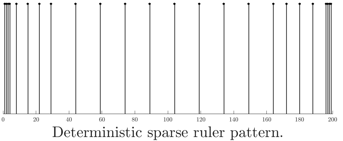
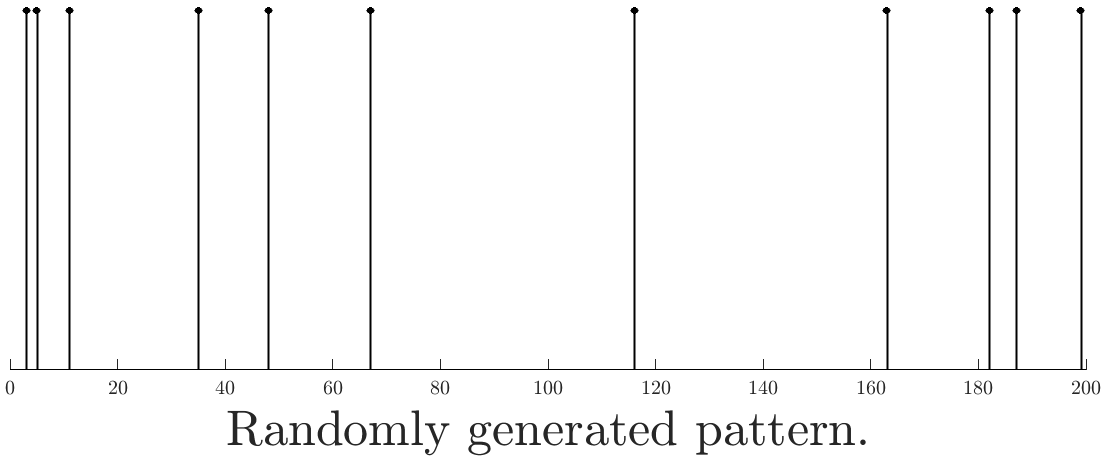
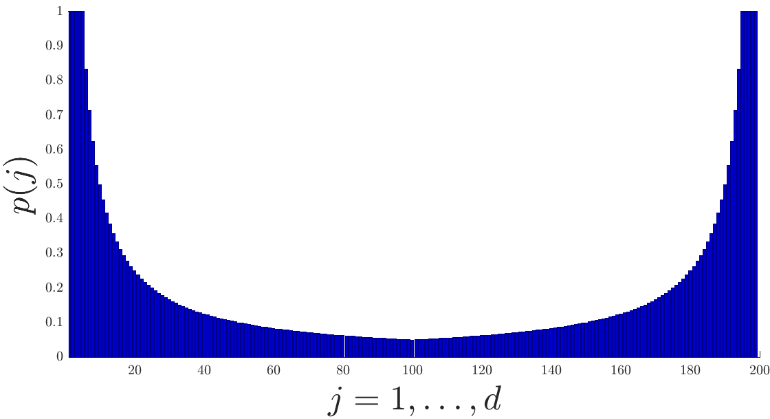
Figure 4: In Section 5, we introduce a strategy that chooses a fixed sampling pattern by independently choosing each j∈1,…,dj\in 1,\ldots,d with probability p⁡(j)p(j), for an explicit function pp (see Algorithm 3). Roughly, p⁡(j)∼1/min⁡(d−j,j)p(j)\sim 1/\min(d-j,j), so samples closer to the edges of 1,…,d1,\ldots,d are selected with higher probability. This produces a pattern that intuitively looks like many sparse rulers, but can be much sparser (see Figure 5).

Specifically, the powerful Vandermonde decomposition theorem [CF11, Pis73] (see Fact 3.1) implies a connection between low-rank Toeplitz matrices and Fourier sparse functions: TT is rank-kk if and only if its columns are spanned by kk vectors obtained from evaluating kk complex sinusoids on the integer grid 0,…,d−10,\ldots,d-1. I.e., every column of TT has a kk-sparse Fourier representation (with arbitrary frequencies in the range [0,1][0,1]) and it follows that any sample x(ℓ)∼𝒩⁡(0,T)x^{(\ell)}\sim\mathcal{N}(0,T) does as well.

This observation allows for a resolution of the question above. In particular, Prony’s method [DP95] implies that any sum of kk complex sinusoids can be recovered from exactly 2​k2k values. Accordingly, when TT is exactly rank-kk, we can select 2​k2k arbitrary entries in x(ℓ)x^{(\ell)}, use Prony’s method to recover the remaining entries, and run our algorithm from Theorem 2.4 to approximate TT. This approach achieves sample complexity linear in kk and logarithmic in dd. In Section 5 we improve the logarithmic dependence to obtain a result that is fully independent of the dimension:

Theorem 2.9 (Dimension indep. complexity via Prony’s method).

For any positive semidefinite Toeplitz matrix T∈ℝd×dT\in\R^{d\times d} with rank kk, Problem 2.1 can be solved by Algorithm 2 with vector sample complexity O⁡(log⁡(k/δ)ε2)O\left(\frac{\log(k/\delta)}{\varepsilon^{2}}\right), entry sample complexity Θ⁡(k)\Theta(k), and total sample complexity O⁡(k​log⁡(k/δ)ε2)O\left(\frac{k\log(k/\delta)}{\varepsilon^{2}}\right).

Unfortunately, Prony’s method is notoriously sensitive to noise [SP95]: it fails to recover a sum of kk complex sinusoids from 2​k2k values when those values are perturbed by even a very small amount of noise. The effect in our setting is that Theorem 2.9 relies heavily on TT being exactly rank-kk.

To handle the more typical case when TT is only close to low-rank, we first prove that in this setting, TT is still closely approximated by a kk-sparse Fourier representation. We then build on recent work on provably interpolating Fourier sparse functions with noise [CKPS16, CP18] to show how to recover this representation. Our proofs leverage several tools from randomized numerical linear algebra, including column subset selection bounds and the projection-cost preserving sketches of [CEM+15].

While this approach is somewhat involved (see Section 5 for the full development) a key takeaway is how it collects samples from each x(ℓ)x^{(\ell)}. In contrast to ruler based methods, we generate a fixed pattern based on randomly sampling a subset of entries in 1,…,d1,\ldots,d (see Figure 4). The randomized strategy concentrates samples near the edges of 1,…,d1,\ldots,d, producing a pattern that is intuitively similar to many sparse ruler designs, but much sparser. Overall, we obtain:

Theorem 2.10 (Sparse Fourier trans. sample complexity).

For any positive semidefinite Toeplitz matrix T∈ℝd×dT\in\R^{d\times d} with rank kk, Problem 2.1 can be solved with failure probability δ≤110\delta\leq\frac{1}{10} by Algorithm 3 with vector sample complexity O⁡(log⁡d​log⁡(d/ε)ε2+k)O\left(\frac{\log d\log(d/\varepsilon)}{\varepsilon^{2}}+k\right) and entry sample complexity Θ⁡(k2​log⁡k​log⁡(d/ε))\Theta(k^{2}\log k\log(d/\varepsilon)). The same bounds hold when TT is close to low-rank, with (∥T−Tk∥2+tr⁡(T−Tk)k)⋅tr⁡(T)=O⁡(ε2​‖T‖22)\left(\lVert T-T_{k}\rVert_{2}+\frac{\mathrm{tr}(T-T_{k})}{k}\right)\cdot\mathrm{tr}(T)=O(\varepsilon^{2}\left\lVert T\right\rVert_{2}^{2}).

See Section 5 for a full statement of Theorem 2.10. As a corollary, in Theorem 5.8, we also give a bound with sample complexity depending polynomially on the stable rank of TT, s=tr⁡(T)∥T∥2s=\frac{\mathrm{tr}(T)}{\lVert T\rVert_{2}}.

Refer to caption
Refer to caption
Figure 5: The left image depicts the minimum size (s=24s=24) sparse ruler for d=199d=199 [Wic63]. The right image depicts a randomly sampled set of s=12s=12 nodes that can be used in the algorithms from Section 5. After random generation, the same pattern is used for selecting entries in each vector x(1),…,x(n)∼𝒩⁡(0,T)x^{(1)},\ldots,x^{(n)}\sim\mathcal{N}(0,T). Like the sparse ruler, the random pattern concentrates nodes towards the end points of 1,…,d1,\ldots,d. See Figure 4 for more details.

We believe that improving Theorem 2.10 is an interesting and potentially impactful direction for future work. For example, it may be possible to improve the dependence on kk in the total sample complexity. We do give two incomparable lower bounds which argue that at least a linear dependence on kk is unavoidable. The first is against any non-adaptive algorithm:

Theorem 2.11 (Informal, see Theorem 6.1).

Any algorithm that solves Problem 2.1 for any rank-kk Toeplitz matrix T∈ℝd×dT\in\R^{d\times d} by inspecting the entries of nn samples x(1),…,x(n)x^{(1)},\ldots,x^{(n)} non-adaptively (i.e. the algorithm chooses, possibly randomly, a fixed set of positions to be read before seeing the samples), has total sample complexity Ω⁡(k/log⁡k)\Omega(k/\log k).

In particular, all of our upper bounds use non-adaptive sampling strategies, and so this theorem shows that they cannot be improved beyond potentially a O~​(k2)\tilde{O}(k^{2}) factor. We further demonstrate that even adaptive algorithms cannot avoid this lower bound, if a small amount of noise is added:

Theorem 2.12 (Informal, see Theorem 6.6).

Any algorithm that solves Problem 2.1 for any approximately rank-kk Toeplitz matrix T∈ℝd×dT\in\R^{d\times d}, by inspecting the entries of nn samples in a potentially adaptive manner, has total sample complexity Ω⁡(k)\Omega(k).

For the formal definition of what it means to be “approximately rank-kk” in this context, see Theorem 6.6. The proof of this is inspired by lower bounds on sparse Fourier transforms and goes via information theory. We highlight one particularly interesting consequence of these bounds. By taking k=Ω⁡(d)k=\Omega(d) in the above lower bounds, one immediately obtains that no algorithm (even potentially adaptive), can avoid total sample complexity Ω⁡(d)\Omega(d) for Problem 2.1, without any rank constraints. Thus, in the metric of TSC, with no rank constraints, the simple algorithm of Theorem 2.4 is in nearly optimal for Problem 2.1. See Section 6 for a more detailed discussion.

2.4 Related work

The problem of estimating Toeplitz covariance matrices using all dd entries of each sample x(ℓ)x^{(\ell)} is a classical statistical problem. Methods for finding maximum likelihood or minimax estimators have been studied in a variety of settings [Bur67, KM81, BLW82] and we refer the reader to [BS97] for an overview. These methods seek to extract a Toeplitz matrix from the sample covariance to improve estimation performance. Existing approaches range from very simple (e.g., diagonal averaging as in our Theorem 2.4 [CRZ13]) to more complex (e.g., EM-like methods [MS87]). We are not aware of any work that establishes a generic non-asymptotic bound like Theorem 2.4.

Work on Toeplitz covariance estimation with the goal of minimizing entry sample complexity has focused on sparse ruler based sampling. This approach has been known for decades [Mof68, PBNH85] and is widely applied in signal processing applications: we refer the reader to [RATL16] for an excellent overview. There has been quite a bit of interest in finding rulers of minimal size – asymptotically, Θ⁡(d)\Theta(\sqrt{d}) is optimal, but in many applications minimizing the leading constant is important [Lee56, Wic63, RSTL88]. There has been less progress on understanding rates of convergence for sparse ruler methods. [WZY17] provides some initial results on bounding ‖T−T~‖2\|T-\tilde{T}\|_{2}, but we are not aware of any strong relative error bounds like those of Theorem 2.6 or Theorem 2.8. [QP17] gives the closest analog, proving non-asymptotic vector sample complexity bounds for sparse ruler sampling. They measure error in terms of the ℓ2\ell_{2} norm of the first column of TT, which can be translated to a Frobenius norm bound of the form ∥T−T~∥F≤ϵ​∥T∥F\lVert T-\tilde{T}\rVert_{F}\leq\epsilon\lVert T\rVert_{F}, but not directly to a spectral norm bound.

More related to the algorithmic contributions of Section 5, are methods that make the additional assumption that TT is low-rank, or close to low-rank. The most well-known algorithms in this setting are the MUSIC [Sch81, Sch86, Pis73] and ESPRIT methods [RK89], although other approaches have been studied [BM86, FB96, ME09]. As discussed, Toeplitz TT is low-rank exactly when its columns are Fourier sparse functions. Accordingly, such methods are closely related to sparse recovery algorithms for “off-grid” frequencies. Most theoretical bounds for “off-grid” sparse recovery require strong separation assumptions that no frequencies are too close together [TBSR13, CFG14, TBR15, BCG+15]. A recent exception is [CKPS16], which we build on in this work since a lack of separation assumptions is essential to obtaining bounds for general low-rank Toeplitz matrices. Under separation assumptions on the frequencies in TT’s Vandermonde decomposition, we note that [QP17] gives an algorithm with O⁡(k)O(\sqrt{k}) ESC and poly⁡(d,k,ϵ)\poly(d,k,\epsilon) VSC when TT is close to rank-kk, using a sparse recovery based approach.

Finally, we note that covariance estimation where <d<d entries of x(l)x^{(l)} are available has been studied without a Toeplitz assumption [GRESS16]. Without Toeplitz and thus Fourier structure, this work is more closely related to the matrix completion problem [CR09] than our setting.

2.5 Open questions

Our work initiates a comprehensive study of non-asymptotic complexity bounds for the recovery of Toeplitz covariance matrices, and leaves a number of open questions.

Efficiency. All of our estimators run in polynomial time except for Algorithm 3, which is used to obtain the bound of Theorem 2.10. An interesting open question is if one can use techniques from e.g., [CKPS16] to obtain polynomial time estimators for this setting.

Tighter bounds. While we present non-asymptotic sample complexity upper and lower bounds for many of the settings considered in this paper, and they are within polynomial factors of each other, it is an interesting open question to exactly characterize the sample complexities of these problems and to fully understand the tradeoffs between entry and vector sample complexity. Moreover, it is unclear if the form of the tail error we obtain for approximately rank-kk Toeplitz matrices is optimal, and it would be interesting to understand this better. A particularly interesting question is if the O⁡(k)O(\sqrt{k}) entry sample complexity bound of [QP17] can be obtained for general low-rank TT, without the additional assumptions made in that work.

Other settings / measures of error. It would be interesting to consider continuous analogs of this problem, for instance, on continuous or infinite length stationary signals. There has been substantial recent work on this subject [CTE18, AL12, LDTN11], and we believe that similar insights can be brought to bear here. There are also other interesting measures of error, for instance, relative Loewner ordering, or total variation distance the sampled and estimated distributions, which corresponds to recovering TT in the so-called Mahalanobis distance. Many of our results can be directly applied to these settings when TT is well-conditioned. However, it would be interesting to understand the sample complexities of these problems in more detail.

3 Notation and Preliminaries

Indexing. For a postive integer zz let [z]:={1,…,z}[z]\vcentcolon=\{1,\ldots,z\}. For a set SS, let SzS^{z} denote the set of subsets of SS with zz elements. For a vector v∈ℂdv\in\C^{d}, let vS∈ℝ|S|v_{S}\in\R^{|S|} denote the restriction of vv to the coordinates in SS. For T∈ℝd×dT\in\R^{d\times d} and set R⊆[d]R\subseteq[d] let TR∈ℝ|R|×|R|T_{R}\in\R^{|R|\times|R|} denote the principle submatrix of TT with rows and columns indexed by RR. Note that even when TT is Toeplitz, TRT_{R} may not be.

Toeplitz matrix operations. For any vector a=[a0,…,ad−1]∈ℝda=[{a}_{0},\ldots,{a}_{d-1}]\in\R^{d}, let Toep⁡(a)∈ℝd×d\mathrm{Toep}(a)\in\R^{d\times d} denote the symmetric Toeplitz matrix whose entries are Toep​(a)j,k=a|j−k|\mathrm{Toep}(a)_{j,k}=a_{|j-k|}. For any M∈ℝd×dM\in\R^{d\times d}, let diag⁡(M)\mathrm{diag}(M) be the matrix given by setting all of MM’s off diagonal entries to 00. Let avg⁡(M)\mathrm{avg}(M) be the symmetric Toeplitz matrix given by averaging the diagonals of MM. Namely, avg⁡(M)=Toep⁡(a)\mathrm{avg}(M)=\mathrm{Toep}(a) where for s∈{0,…​d−1}s\in\{0,\ldots d-1\}, as=1|j,k∈[d]:|j−k|=s|∑j,k∈[d]:|j−k|=sMj,ka_{s}=\frac{1}{\left|j,k\in[d]:|j-k|=s\right|}\sum_{j,k\in[d]:|j-k|=s}M_{j,k}.

Linear algebra notation. For a matrix AA, let ATA^{T} and A∗A^{*} denote the transpose and Hermitian transpose, respectively. When all of AA’s entries are real, A∗=ATA^{*}=A^{T}. For a vector y∈ℂdy\in\C^{d} let ‖y‖2=y∗​y\|y\|_{2}=\sqrt{y^{*}y} denote the ℓ2\ell_{2} norm. For a matrix AA with dd columns, let ‖A‖2=supx∈Cd‖A​x‖2/‖x‖2\|A\|_{2}=\sup_{x\in C^{d}}\|Ax\|_{2}/\|x\|_{2} denote spectral norm. Let ‖A‖F\|A\|_{F} denote the Frobenius norm.

A Hermitian matrix A∈ℂd×dA\in\C^{d\times d} is positive semidefinite (PSD) if for all x∈ℂdx\in\C^{d}, x∗​A​x≥0x^{*}Ax\geq 0. Let ⪯\preceq denote the Loewner ordering: A⪯BA\preceq B indicates that B−AB-A is PSD. Let A+A^{+} denote the Moore-Penrose pseudoinverse of AA. A+=V​Σ−1​U∗A^{+}=V\Sigma^{-1}U^{*} where U​Σ​V∗=AU\Sigma V^{*}=A is the compact singular value decomposition of AA. When AA is PSD, let A1/2=U​Σ1/2A^{1/2}=U\Sigma^{1/2} where Σ1/2\Sigma^{1/2} is obtained by taking the entrywise square root of Σ.\Sigma. Let AkA_{k} denote the projection of AA onto its top kk-singular vectors: Ak=Uk​Σk​Vk∗A_{k}=U_{k}\Sigma_{k}V_{k}^{*} where Uk,Vk∈ℂd×kU_{k},V_{k}\in\C^{d\times k} contain the first kk columns of U,VU,V respectively and Σk∈ℝk×k\Sigma_{k}\in\R^{k\times k} is diagonal matrix containing AA’s largest kk singular values. Note that AkA_{k} is an optimal low-rank approximation in that: Ak=arg​minrank​k​M⁡∥A−M∥F=arg​minrank​k​M⁡∥A−M∥2A_{k}=\argmin_{\mathrm{rank}\,k\ M}\lVert A-M\rVert_{F}=\argmin_{\mathrm{rank}\,k\ M}\lVert A-M\rVert_{2}.

Gaussians, TV distance, KL divergence. We let x∼𝒩⁡(m,T)x\sim\mathcal{N}(m,T) indicates that xx is drawn from a Gaussian distribution with mean mm and covariance TT. When B∈ℂd×dB\in\C^{d\times d}, it is an elementary fact that x∼𝒩⁡(0,BB∗)x\sim\normal(0,BB^{*}), can be written as x=B​U​gx=BUg where g∼𝒩⁡(0,I)g\sim\normal(0,I) and U∈ℂd×dU\in\C^{d\times d} is a fixed unitary matrix. When BB is real, UU can be any orthogonal matrix in ℝd×d\R^{d\times d}. For any two distributions F,GF,G, let dTV​(F,G)=12​∫|𝑑F−𝑑G|d_{\mathrm{TV}}(F,G)=\frac{1}{2}\int|dF-dG| denote their total variation distance, and let dKL​(F,G)=∫log⁡d​Fd​G​𝑑Fd_{\mathrm{KL}}(F,G)=\int\log\frac{dF}{dG}dF denote the KL divergence [CT12].

Probability notation. We let Pr⁡[g]\Pr[g] denote the probability that event gg occurs. Sometimes we add an additional subscript to remind the reader of any random events that effect gg, and thus its probability. For example, we might write Prx⁡[g]\Pr_{x}[g] if xx is a random variable and gg depends on xx. We use :: to denote “such that”. For example, Pr[∃x∈𝒳:x>10]\Pr[\exists x\in\mathcal{X}:x>10] denotes the “probability that there exists some element xx in the set 𝒳\mathcal{X} such that xx is greater than 1010.”

Miscellaneous. Let |z|=z∗​z|z|=\sqrt{z^{*}z} denote the magnitude of a complex number zz. Let ii denote −1\sqrt{-1}. When stating asymptotic bounds we use O~​(f)\tilde{O}(f) as shorthand for O⁡(f​logc​f)O(f\log^{c}f) for some constant cc, and similarly we let Ω~​(f)=Ω⁡(f/logc⁡f)\widetilde{\Omega}(f)=\Omega(f/\log^{c}f) for some fixed cc.

3.1 Fourier analytic tools

We repeatedly make use of the Fourier structure of Toeplitz matrices. To that end, we often work with asymmetric Fourier transform matrices whose rows correspond to “on-grid” integer points (e.g., samples in time domain) and whose columns correspond to “off-grid” frequencies.

Definition 3.1 (Fourier matrix).

For a set S={f1,…​fs}⊂ℂS=\{f_{1},\ldots f_{s}\}\subset\C, we define the Fourier matrix FS∈ℂd×sF_{S}\in\C^{d\times s} as the matrix with jthj^{\text{th}} column given by F⁡(fj)F(f_{j}), where:

F​(fj)⊤=[1,e−2​π​i​fj,e−2​π​i​2​fj,…,e−2​π​i​(d−1)​fj].\displaystyle F(f_{j})^{\top}=\left[1,e^{-2\pi if_{j}},e^{-2\pi i2f_{j}},\ldots,e^{-2\pi i(d-1)f_{j}}\right].

While Toeplitz matrices cannot in general be diagonalized by the discrete Fourier transform like circulant matrices, the Carathéodory-Fejér-Pisarenko decomposition (also known as the Vandermonde decomposition) implies that they can be diagonalized by a Fourier matrix with off-grid frequencies [CF11, Pis73]. A general version of the classical result holding for all ranks r≤dr\leq d is:

Fact 3.1 (Vandermonde Decomposition, Cor. 1 of [Cyb82]).

Any PSD Toeplitz matrix T∈ℝd×dT\in\R^{d\times d} with rank r≤dr\leq d can be written as T=FS​D​FS∗T=F_{S}DF_{S}^{*} where D∈ℝr×rD\in\R^{r\times r} is positive and diagonal and FS∈ℂd×rF_{S}\in\C^{d\times r} is a Fourier matrix (as in Definition 3.1) with frequencies S={f1,…​fr}⊂[0,1]S=\{f_{1},\ldots f_{r}\}\subset[0,1]. Furthermore, f1,…​frf_{1},\ldots f_{r} come in conjugate pairs with equal weights: i.e., for every j∈[r]j\in[r], there is a j′j^{\prime} (possibly with j′=jj^{\prime}=j) with e−2​π​i​fj=e2​π​i​fj′e^{-2\pi if_{j}}=e^{2\pi if_{j^{\prime}}} and Dj,j=Dj′,j′D_{j,j}=D_{j^{\prime},j^{\prime}}.

One useful consequence of the Vandermonde decomposition is that, as d→∞d\rightarrow\infty, TT is diagonalized by the discrete time Fourier transform. We can take advantage of this property by noting that any Toeplitz matrix Toep⁡(a)\mathrm{Toep}(a) can be extended to be arbitrarily large by padding aa with 00’s. The spectral norm of the extension upper bounds that of Toep⁡(a)\mathrm{Toep}(a). Accordingly, we can bound ‖Toep⁡(a)‖2\|\mathrm{Toep}(a)\|_{2} by the supremum of aa’s DTFT. We refer the reader to [Mec07] for a formal argument, ultimately giving:

Fact 3.2 (See e.g., [Mec07]).

For any a=[a0,…,ad−1]∈ℝda=[a_{0},\ldots,a_{d-1}]\in\R^{d},

‖Toep⁡(a)‖2\displaystyle\|\mathrm{Toep}({a})\|_{2} ≤supx∈[0,1]La​(x)\displaystyle\leq\sup_{x\in[0,1]}L_{a}(x) where La​(x)\displaystyle L_{{a}}(x) :=a0+2∑s=1d−1ascos(2πsx).\displaystyle\vcentcolon={a}_{0}+2\sum_{s=1}^{d-1}{a}_{s}\cos(2\pi sx).

3.2 Linear algebra tools

Our methods with sample complexity logarithmic in dd for low-rank (or close to low-rank) TT do not select entries from each x∼𝒩⁡(0,T)x\sim\mathcal{N}(0,T) according to a fixed pattern like a sparse ruler. Instead, they use a randomly chosen pattern. We view this approach as randomly selecting a subset of rows from the d×nd\times n matrix of samples [x(1),…,x(n)][x^{(1)},\ldots,x^{(n)}]. To find a subset that preserves properties of this matrix, we turn to tools from randomized numerical linear algebra and matrix sketching [Mah11, DM16]. Specifically, we adapt ideas from random selection algorithms based on importance sampling – i.e., when rows are sampled independently at random with non-uniform probabilities.

In particular, work on matrix sketching and graph sparsification has repeatedly used importance sampling probabilities proportional to the statistical leverage scores [SS11, DMM06], which allow for random matrix compressions that preserve significant information [CEM+15, MM17]. Formally, the leverage score is a measure defined for any row in a matrix A∈ℂd×sA\in\C^{d\times s}:

Definition 3.2.

The leverage score, τj​(A)\tau_{j}(A), of the jthj^{\text{th}} row aj∈ℂd×1a_{j}\in\C^{d\times 1} in A∈ℂd×sA\in\C^{d\times s} is defined as:

τj​(A):=aj​(A∗​A)+​aj∗.\displaystyle\tau_{j}(A)\vcentcolon=a_{j}\left(A^{*}A\right)^{+}a_{j}^{*}.

Note that that ∑j=1dτj​(A)=tr⁡(A​(A∗​A)+​A∗)=rank⁡(A)≤min⁡(d,s)\sum_{j=1}^{d}\tau_{j}(A)=\mathrm{tr}\left(A\left(A^{*}A\right)^{+}A^{*}\right)=\mathrm{rank}(A)\leq\min(d,s).

The leverage score can be seen as measuring the “uniqueness” of any row. This intuition is captured by the following lemmas, which are used extensively in prior work on leverage scores:

Fact 3.3 (Minimization Characterization).
τj​(A)=miny∈ℂd⁡ s.t. ​yT​A=aj⁡‖y‖22.\displaystyle\tau_{j}(A)=\min_{y\in\C^{d}\text{ s.t. }y^{T}A=a_{j}}\|y\|_{2}^{2}.
Fact 3.4 (Maximization Characterization).

Let (A​y)j\left(Ay\right)_{j} denote the jthj^{\text{th}} entry of the vector A​yAy.

τj​(A)=maxy∈ℂs⁡|(A​y)j|2∥A​y∥22.\displaystyle\tau_{j}(A)=\max_{y\in\C^{s}}\frac{\left|\left(Ay\right)_{j}\right|^{2}}{\lVert Ay\rVert_{2}^{2}}.

One consequence of Fact 3.3 is that τj​(A)≤1\tau_{j}(A)\leq 1 for all jj since we can choose yy to be the jthj^{\text{th}} standard basis vector. We defer further discussion and proofs of these bounds to Appendix A, where we also state a standard matrix concentration bound for sampling by leverage scores.

In our applications, we cannot compute leverage scores explicitly, since we use them to sample rows from [x(1),…,x(n)][x^{(1)},\ldots,x^{(n)}] without ever looking at this whole matrix. To cope with this challenge we take advantage of the Fourier structure of Toeplitz matrices (Claim 3.1), which ensures that each x(ℓ)x^{(\ell)} can be written as a Fourier sparse or nearly Fourier sparse function when TT is low-rank or close to low-rank. This allows us to extend recent work on nearly tight a priori leverage scores estimates for Fourier sparse matrices [CKPS16, CP18, CP19, AKM+19] to our setting. See Appendix A.

3.3 Distances between Gaussians

In our lower bound proofs, we repeatedly use the following bounds on the TV distance and KL divergence between Gaussians.

Fact 3.5.

Let M1,M2∈ℝd×dM_{1},M_{2}\in\R^{d\times d} be PSD. Then,

dKL(𝒩(0,M1),𝒩(0,M2))=Θ(‖I−M2−1/2M1M2−1/2‖F2).\displaystyle d_{\mathrm{KL}}(\normal(0,M_{1}),\normal(0,M_{2}))=\Theta\left(\left\lVert I-M_{2}^{-1/2}M_{1}M_{2}^{-1/2}\right\rVert_{F}^{2}\right)\;.

By Pinsker’s inequality [CT12], this implies that

dTV(𝒩(0,M1),𝒩(0,M2))=O(‖I−M1−1/2M2M1−1/2‖F).\displaystyle d_{\mathrm{TV}}(\normal(0,M_{1}),\normal(0,M_{2}))=O\left(\left\lVert I-M_{1}^{-1/2}M_{2}M_{1}^{-1/2}\right\rVert_{F}\right)\;.

3.4 Concentration bounds

We make use of the following well known concentration inequality for quadratic forms:

Claim 3.6 (Hanson-Wright Inequality – see e.g., [RV13]).

Let x(1),…,x(n)∼𝒩⁡(0,I)x^{(1)},\ldots,x^{(n)}\sim\normal(0,I) be independent. There exists a universal constant c>0c>0 so that for all A∈ℝd×dA\in\R^{d\times d} and all t>0t>0,

Pr[|1n∑ℓ=1nx(ℓ)TAx(ℓ)−tr(A)|>t]≤2exp(−c⋅nmin(t2‖A‖F2,t‖A‖2)).\displaystyle\Pr\left[\left|\frac{1}{n}\sum_{\ell=1}^{n}{x^{(\ell)}}^{T}Ax^{(\ell)}-\mathrm{tr}(A)\right|>t\right]\leq 2\exp\left(-c\cdot n\min\left(\frac{t^{2}}{\|A\|_{F}^{2}},\frac{t}{\|A\|_{2}}\right)\right)\;.

4 Covariance Estimation by Ruler

We begin by establishing Theorems 2.4 and 2.6, which can be analyzed in a unified way. In particular, both bounds are achieved by Algorithm 1 (see below) with the ruler RR chosen to either equal [d][d] for Theorem 2.4, or to be a suitable sparse ruler for Theorem 2.6 (see Definition 2.1). Algorithm 1 approximates T=Toep⁡(a)T=\mathrm{Toep}(a) by individually approximating each entry as{a}_{s} in aa by an average over all entries in each x(j)x^{(j)} with distance ss from each other. Letting a~{\tilde{a}} denote this approximation, the algorithm returns the Toeplitz matrix T~=Toep⁡(a~)\tilde{T}=\mathrm{Toep}({\tilde{a}}).

Algorithm 1 Toeplitz covariance estimation by ruler

input: Independent samples x(1),…,x(n)∼𝒩⁡(0,T)x^{(1)},\ldots,x^{(n)}\sim\mathcal{N}(0,T).
parameters: Ruler R⊆[d]R\subseteq[d].
output: T~∈ℝd×d\tilde{T}\in\R^{d\times d} approximating TT.


1: for s=0,…,d−1s=0,\ldots,d-1 do
2:   a~s:=1n​|Rs|​∑ℓ=1n∑(j,k)∈Rsxj(ℓ)​xk(ℓ){\tilde{a}}_{s}:=\frac{1}{n|R_{s}|}\sum_{\ell=1}^{n}\sum_{(j,k)\in R_{s}}x^{(\ell)}_{j}x^{(\ell)}_{k},   (where RsR_{s} is defined in Definition 2.1)
3: end for
4: return T~:=Toep⁡(a~)\tilde{T}\vcentcolon=\mathrm{Toep}({\tilde{a}}).

When R=[d]R=[d], Algorithm 1 reduces to approximating TT by the empirical covariance with its diagonals averaged to make it symmetric and Toeplitz. In the other extreme, we can approximate TT using a sparse ruler with |R|=O⁡(d)|R|=O(\sqrt{d}) (see Claim 2.5). It is easy to see the following:

Claim 4.1.

Algorithm 1 has vector sample complexity nn, entry sample complexity |R||R|, and total sample complexity n​|R|n|R|. It runs in time O⁡(n​|R|2)O\left(n|R|^{2}\right) and outputs a symmetric Toeplitz matrix T~\tilde{T}.

We prove a generic bound on the accuracy of Algorithm 1 for any nn and ruler RR (the accuracy will depend on properties of RR). We then instantiate this bound for specific choices of these parameters to give Theorem 2.4, Theorem 2.6, and also Theorem 2.8 when TT is approximately low-rank. We first define a quantity characterizing how extensively a ruler covers distances 0,…,d−10,\ldots,d-1:

Definition 4.1 (Coverage coefficient, Δ⁡(R)\Delta(R)).

For any ruler R⊆[d]R\subseteq[d] let Δ⁡(R):=∑s=0d−11|Rs|.\Delta(R)\vcentcolon=\sum_{s=0}^{d-1}\frac{1}{|R_{s}|}.

The coverage coefficient of a ruler is smaller when distances are represented more frequently by the ruler, so intuitively, the sample complexity will scale with it. It is not hard to check that when R=[d]R=[d], Δ⁡(R)=Θ⁡(log⁡d)\Delta(R)=\Theta(\log d) and for any RR with |R|=Θ⁡(d)|R|=\Theta(\sqrt{d}), Δ⁡(R)=Θ⁡(d)\Delta(R)=\Theta(d). It is also possible to construct rulers which interpolate between Θ⁡(d)\Theta(\sqrt{d}) and dd sparsity:

Definition 4.2.

For α∈[1/2,1]\alpha\in[1/2,1], let RαR_{\alpha} be the ruler given by Rα=Rα(1)∪Rα(2)R_{\alpha}=R^{(1)}_{\alpha}\cup R^{(2)}_{\alpha}, where44 4 We assume for simplicity of exposition that dαd^{\alpha} and d1−αd^{1-\alpha} are integers.

Rα(1)={1,2,…,dα},and​Rα(2)={d,d−d1−α,d−2​d1−α,…,d−(dα−1)​d1−α}.R^{(1)}_{\alpha}=\{1,2,\ldots,d^{\alpha}\}\;,~\mbox{and}~\;R^{(2)}_{\alpha}=\{d,d-d^{1-\alpha},d-2d^{1-\alpha},\ldots,d-(d^{\alpha}-1)d^{1-\alpha}\}\;. (1)

For such rulers we prove the following general bound in Appendix B:

Lemma 4.2.

For any α∈[1/2,1]\alpha\in[1/2,1], RαR_{\alpha} has size |Rα|≤2​dα|R_{\alpha}|\leq 2d^{\alpha}, and moreover

Δ⁡(Rα)≤2​d2−2​α+d1−α​(1+log⁡(⌈d2​α−1⌉))=d2−2​α+O⁡(d1−α⋅log⁡d).\displaystyle\Delta(R_{\alpha})\leq 2d^{2-2\alpha}+d^{1-\alpha}(1+\log(\lceil d^{2\alpha-1}\rceil))=d^{2-2\alpha}+O(d^{1-\alpha}\cdot\log d)\;.

Note that for α=1\alpha=1 we recover a bound of O⁡(log⁡d)O(\log d) and for α=1/2\alpha=1/2 a bound of O⁡(d)O(d). With the coverage coefficient defined, we prove our general bound for any ruler RR:

Theorem 4.3 (Accuracy of Algorithm 1).

Let T~\tilde{T} be the output of Algorithm 1 run with ruler RR. For any ε∈(0,1]\varepsilon\in(0,1], let κ:=min⁡(1,ε2⋅∥T∥22Δ⁡(R)⋅∥TR∥22)\kappa\vcentcolon=\min\left(1,\frac{\varepsilon^{2}\cdot\lVert T\rVert_{2}^{2}}{\Delta(R)\cdot\lVert T_{R}\rVert_{2}^{2}}\right). There exist universal constants C,c>0C,c>0 such that

Pr[‖T−T~‖2>ε∥T∥2]≤C​d2εexp(−cnκ).\displaystyle\Pr\left[\left\|T-\tilde{T}\right\|_{2}>\varepsilon\lVert T\rVert_{2}\right]\leq\frac{Cd^{2}}{\varepsilon}\exp\left(-cn\kappa\right)\;.

In particular, if n=Θ⁡(log⁡(d/ε​δ)κ)n={\Theta}\left(\frac{\log\left({d/\varepsilon\delta}\right)}{\kappa}\right), then ‖T−T~‖2≤ε​∥T∥2\left\|T-\tilde{T}\right\|_{2}\leq\varepsilon\lVert T\rVert_{2} with probability at least 1−δ1-\delta.

Proof.

As noted in Claim 4.1, T~\tilde{T} is a symmetric Toeplitz matrix and so T−T~T-\tilde{T} is a symmetric Toeplitz matrix. Let e∈ℝde\in\R^{d} be its associated vector, so that ee is a random variable. By Fact 3.2, to prove the theorem it suffices to show that there exist C,c>0C,c>0 with:

Pre[∃x∈[0,1]:|Le(x)|≥ε∥T∥2]≤C​d2εexp(−cnκ).\displaystyle\Pr_{e}\left[\exists x\in[0,1]:|L_{e}(x)|\geq\varepsilon\lVert T\rVert_{2}\right]\leq\frac{Cd^{2}}{\varepsilon}\exp\left(-cn\kappa\right)\;.

Let N={0,εQ​d2,2​εQ​d2,…,1}N=\{0,\frac{\varepsilon}{Qd^{2}},\frac{2\varepsilon}{Qd^{2}},\ldots,1\}, for some universal constant QQ sufficiently large (Q=80​πQ=80\pi suffices). We will prove that there exists a universal constant c>0c>0 so that the following two bounds hold:

Pre[∃s∈{0,…,d−1}:|es|>10∥T∥2]\displaystyle\Pr_{{e}}\left[\exists s\in\{0,\ldots,d-1\}:|{e}_{s}|>10\|T\|_{2}\right] ≤exp⁡(−c​n), and\displaystyle\leq\exp(-cn)\;,\;\mbox{ and } (2)
Pre[∃x∈N:|Le(x)|>ε2∥T∥2]\displaystyle\Pr_{e}\left[\exists x\in N:|L_{e}(x)|>\frac{\varepsilon}{2}\|T\|_{2}\right] ≤3​Q​d2ε​exp⁡(−c​n​κ).\displaystyle\leq\frac{3Qd^{2}}{\varepsilon}\exp\left(-cn\kappa\right)\;. (3)

We first show how (2) and (3) together imply the desired bound. Condition on the event that |es|≤10​‖T‖2|{e}_{s}|\leq 10\|T\|_{2} for all ss and the event that |Le​(x)|≤ε2​‖T‖2|L_{e}(x)|\leq\frac{\varepsilon}{2}\|T\|_{2} for all x∈Nx\in N. By (2) and (3) and a union bound, we know that this happens with probability at least

1−4​Q​d2ε2​exp⁡(−c​n​κ).\displaystyle 1-\frac{4Qd^{2}}{\varepsilon^{2}}\exp\left(-cn\kappa\right)\;.

Observe that for all x∈[0,1]x\in[0,1], we have

|Le′​(x)|\displaystyle|L_{{e}}^{\prime}(x)| =|4​π⋅∑s=1d−1s⋅es​sin⁡(2​π​s​x)|\displaystyle=\left|4\pi\cdot\sum_{s=1}^{d-1}s\cdot{e}_{s}\sin(2\pi sx)\right|
≤4​π​d2​‖e‖∞≤40​π​d2​‖T‖2,\displaystyle\leq 4\pi d^{2}\|{e}\|_{\infty}\leq 40\pi d^{2}\|T\|_{2},

where in the last line we use that we are conditioning on |es|≤10​∥T∥2|{e}_{s}|\leq 10\lVert T\rVert_{2} for all ss. Now, for any x∈[0,1]x\in[0,1], let x′∈Nx^{\prime}\in N be so that |x−x′|≤ε/(Q​d2)|x-x^{\prime}|\leq\varepsilon/(Qd^{2}). Then, as long as Q≥80​πQ\geq 80\pi, we have

|L⁡(x)−L⁡(x′)|\displaystyle|L(x)-L(x^{\prime})| ≤L⁡(x′)+supy∈[x,x′]|L′​(y)|⋅|x−x′|\displaystyle\leq L(x^{\prime})+\sup_{y\in[x,x^{\prime}]}|L^{\prime}(y)|\cdot|x-x^{\prime}|
≤ε2​‖T‖2+40​π​d2​‖T‖2⋅|x−x′|≤ε​‖T‖2,\displaystyle\leq\frac{\varepsilon}{2}\|T\|_{2}+40\pi d^{2}\|T\|_{2}\cdot|x-x^{\prime}|\leq\varepsilon\|T\|_{2},

which proves the theorem, letting and C=4​QC=4Q.

It thus suffices to prove (2) and (3). We first prove (2). We can write for any s∈0,…,d−1s\in 0,\ldots,d-1:

es=as−a~s=1n⋅|Rs|​∑ℓ=1n∑(j,k)∈Rs[Tj,k−xj(ℓ)⋅xk(ℓ)].{e}_{s}={a}_{s}-{\tilde{a}}_{s}=\frac{1}{n\cdot|R_{s}|}\sum_{\ell=1}^{n}\sum_{(j,k)\in R_{s}}\left[T_{j,k}-x^{(\ell)}_{j}\cdot x^{(\ell)}_{k}\right].

Observe that for each ℓ=1,…,n\ell=1,\ldots,n, we have that xj(ℓ)⋅xk(ℓ)x^{(\ell)}_{j}\cdot x^{(\ell)}_{k} is a subexponential random variable with mean Tj,kT_{j,k} and second moment which can be written using Isserlis’s theorem as

𝔼[(xj(ℓ))2⋅(xk(ℓ))2]=Tj,j​Tk,k+2​Tj,k2≤3​‖T‖22.\displaystyle\E\left[(x^{(\ell)}_{j})^{2}\cdot(x^{(\ell)}_{k})^{2}\right]=T_{j,j}T_{k,k}+2T_{j,k}^{2}\leq 3\|T\|_{2}^{2}.

The desired bound then follows from standard bounds on subexponential random variables [Wai19].

We now turn our attention to (3). Fix x∈[0,1]x\in[0,1], and associate to it the Toeplitz matrix M∈ℝd×dM\in\R^{d\times d}, where for all s∈0,…,d−1s\in 0,\ldots,d-1 and (j,k)∈[d]×[d](j,k)\in[d]\times[d] with |j−k|=s|j-k|=s, we let

Mj,k=cos⁡(2​π​s​x)|Rs|.\displaystyle M_{j,k}=\frac{\cos(2\pi sx)}{|R_{s}|}.

Letting T¯\overline{T} be the empirical covariance matrix T¯:=1n​∑ℓ=1nx(ℓ)​x(ℓ)T\overline{T}\vcentcolon=\frac{1}{n}\sum_{\ell=1}^{n}x^{(\ell)}{x^{(\ell)}}^{T}, we can see that

Le​(x)=e0+2​∑s=1d−1es​cos⁡(2​π​s​x)=tr⁡(TR−T~R,MR)=tr⁡(TR−T¯R,MR).\displaystyle L_{e}(x)={e}_{0}+2\sum_{s=1}^{d-1}{e}_{s}\cos(2\pi sx)=\mathrm{tr}(T_{R}-\tilde{T}_{R},M_{R})=\mathrm{tr}(T_{R}-\overline{T}_{R},M_{R}). (4)

The last equality follows from the fact that MM is symmetric Toeplitz and T~R\tilde{T}_{R} is just obtained by averaging the diagonal entries of T¯R\overline{T}_{R}. That is, for any s∈0,…​d−1s\in 0,\ldots d-1,

∑(j,k)∈R×R:|j−k|=sT~j,k=∑(j,k)∈R×R:|j−k|=sT¯j,k,\displaystyle\sum_{(j,k)\in R\times R:|j-k|=s}\tilde{T}_{j,k}=\sum_{(j,k)\in R\times R:|j-k|=s}\overline{T}_{j,k},

and thus

tr⁡(T~R,MR)\displaystyle\mathrm{tr}(\tilde{T}_{R},M_{R}) =∑(j,k)∈R×RT~j,k⋅Mj,k\displaystyle=\sum_{(j,k)\in R\times R}\tilde{T}_{j,k}\cdot M_{j,k}
=∑s=0d−1[∑(j,k)∈R×R:|j−k|=sT~j,k⋅Mj,k]\displaystyle=\sum_{s=0}^{d-1}\left[\sum_{(j,k)\in R\times R:|j-k|=s}\tilde{T}_{j,k}\cdot M_{j,k}\right]
=∑s=0d−1[∑(j,k)∈R×R:|j−k|=sT¯j,k⋅Mj,k]=tr(T¯R,M).\displaystyle=\sum_{s=0}^{d-1}\left[\sum_{(j,k)\in R\times R:|j-k|=s}\overline{T}_{j,k}\cdot M_{j,k}\right]=\mathrm{tr}(\overline{T}_{R},M).

We will show that for any ε∈[0,1]\varepsilon\in[0,1], there exists c>0c>0 such that:

Pr[|tr(T−T¯R,M)|>ε2∥T∥2]\displaystyle\Pr\left[|\mathrm{tr}(T-\overline{T}_{R},M)|>\frac{\varepsilon}{2}\|T\|_{2}\right] ≤2​exp⁡(−c​n​κ).\displaystyle\leq 2\exp\left(-cn\kappa\right)\;. (5)

Notice that if we let xR(ℓ)∈ℝ|R|x^{(\ell)}_{R}\in\R^{|R|} denote the ℓt​h\ell^{th} sample restricted to the indices in RR we have xR(ℓ)∼𝒩⁡(0,TR)x^{(\ell)}_{R}\sim\normal(0,T_{R}). Therefore, if we let y(ℓ)=TR−1/2x(ℓ)Ry^{(\ell)}=T_{R}^{-1/2}x^{(\ell)}_{R}, the y(ℓ)y^{(\ell)} are i.i.d., with y(ℓ)∼𝒩⁡(0,IR×R)y^{(\ell)}\sim\normal(0,I_{R\times R}). Moreover, we can rewrite the quantity in (5) as:

tr⁡(TR−T¯R,M)\displaystyle\mathrm{tr}(T_{R}-\overline{T}_{R},M) =tr⁡(T,M)−1n​∑i=1nxR(ℓ)T​M​xR(ℓ)\displaystyle=\mathrm{tr}(T,M)-\frac{1}{n}\sum_{i=1}^{n}{x^{(\ell)}_{R}}^{T}Mx^{(\ell)}_{R}
=tr⁡(M′)−1n​∑ℓ=1ny(ℓ)T​M′​y(ℓ),\displaystyle=\mathrm{tr}(M^{\prime})-\frac{1}{n}\sum_{\ell=1}^{n}{y^{(\ell)}}^{T}M^{\prime}y^{(\ell)}\;,

where M′=TR1/2​M​TR1/2M^{\prime}=T_{R}^{1/2}MT_{R}^{1/2}. Observe that ‖M‖F2=∑s=0d−1|Rs|⋅cos⁡(2​π​s​x)2|Rs|2≤Δ⁡(R)\|M\|_{F}^{2}=\sum_{s=0}^{d-1}|R_{s}|\cdot\frac{\cos(2\pi sx)^{2}}{|R_{s}|^{2}}\leq\Delta(R). Additionally, ‖M′‖F≤‖TR‖2​‖M‖F\|M^{\prime}\|_{F}\leq\|T_{R}\|_{2}\|M\|_{F}, and ‖M′‖2≤‖TR‖2​‖M‖2\|M^{\prime}\|_{2}\leq\|T_{R}\|_{2}\|M\|_{2}. Thus, applying the Hanson-Wright inequality (Claim 3.6):

Pr[|tr(TR−T¯R,M)|>ε2∥T∥2]\displaystyle\Pr\left[|\mathrm{tr}(T_{R}-\overline{T}_{R},M)|>\frac{\varepsilon}{2}\|T\|_{2}\right] =Pr[|tr(M′)−1n∑ℓ=1ny(ℓ)TM′y(ℓ)|>ε2∥T∥2]\displaystyle=\Pr\left[\left|\mathrm{tr}(M^{\prime})-\frac{1}{n}\sum_{\ell=1}^{n}{y^{(\ell)}}^{T}M^{\prime}y^{(\ell)}\right|>\frac{\varepsilon}{2}\|T\|_{2}\right]
≤2​exp⁡(−c​n​min⁡(ε2​‖T‖224​‖M′‖F2,ε​‖T‖22​‖M′‖2))\displaystyle\leq 2\exp\left(-cn\min\left(\frac{\varepsilon^{2}\|T\|_{2}^{2}}{4\|M^{\prime}\|_{F}^{2}},\frac{\varepsilon\|T\|_{2}}{2\|M^{\prime}\|_{2}}\right)\right)
≤2​exp⁡(−c​n​min⁡(∥T∥22∥TR∥22⋅ε24​‖M‖F2,∥T∥2∥TR∥2⋅ε2​‖M‖2))\displaystyle\leq 2\exp\left(-cn\min\left(\frac{\lVert T\rVert_{2}^{2}}{\lVert T_{R}\rVert_{2}^{2}}\cdot\frac{\varepsilon^{2}}{4\|M\|_{F}^{2}},\frac{\lVert T\rVert_{2}}{\lVert T_{R}\rVert_{2}}\cdot\frac{\varepsilon}{2\|M\|_{2}}\right)\right)
≤2​exp⁡(−c​n​κ),\displaystyle\leq 2\exp\left(-cn\kappa\right)\;,

recalling that κ:=min⁡(1,ε2⋅∥T∥22Δ⁡(R)⋅∥TR∥22)\kappa\vcentcolon=\min\left(1,\frac{\varepsilon^{2}\cdot\lVert T\rVert_{2}^{2}}{\Delta(R)\cdot\lVert T_{R}\rVert_{2}^{2}}\right). This gives (5). Combining with (4), for any fixed x∈[0,1]x\in[0,1]:

Pr[|Le(x)|>ε∥T∥2]≤2exp(−cnκ),\Pr\left[|L_{e}(x)|>\varepsilon\|T\|_{2}\right]\leq 2\exp\left(-cn\kappa\right)\;, (6)

and so (3) follows by a union bound over all x∈Nx\in N. This completes the proof of Theorem 4.3. ∎

4.1 Applications of the general bound, full rank matrices

We describe a few specific instantiations of Theorem 4.3. When R=[d]R=[d] is the full ruler, Δ⁡(R)=O⁡(log⁡d)\Delta(R)=O(\log d) by Lemma 4.2 and ‖TR‖2=‖T‖2\|T_{R}\|_{2}=\|T\|_{2}. This immediately yields:

Theorem 2.4 (Near linear sample complexity – full theorem).

Let T~\tilde{T} be the output of Algorithm 1 run with the full ruler R=[d]R=[d]. There exist universal constants C,c>0C,c>0 such that, for any ε∈(0,1]\varepsilon\in(0,1]:

Pr[‖T−T~‖2>ε∥T∥2]≤C​d2εexp(−c​n​ε2log⁡d).\displaystyle\Pr\left[\left\|T-\tilde{T}\right\|_{2}>\varepsilon\lVert T\rVert_{2}\right]\leq\frac{Cd^{2}}{\varepsilon}\exp\left(-\frac{cn\varepsilon^{2}}{\log d}\right)\;.

In particular, if n=Ω⁡(log⁡(d/ε​δ)​log⁡dε2)n={\Omega}\left(\frac{\log\left({d}/{\varepsilon\delta}\right)\log d}{\varepsilon^{2}}\right), then ‖T−T~‖2≤ε​∥T∥2\left\|T-\tilde{T}\right\|_{2}\leq\varepsilon\lVert T\rVert_{2} with probability at least 1−δ1-\delta.

We can also apply Theorem 4.3 to any ruler with |R|=Θ⁡(d)|R|=\Theta(\sqrt{d}) (e.g., the ruler in Claim 2.5, or more optimal constructions). In this case, Δ⁡(R)=O⁡(d)\Delta(R)=O(d) and can bound ‖TR‖2≤‖T‖2\|T_{R}\|_{2}\leq\|T\|_{2} to give:

Theorem 2.6 (Sparse ruler sample complexity – full theorem).

Let T~\tilde{T} be the output of Algorithm 1 run with any Θ⁡(d)\Theta(\sqrt{d})-sparse ruler RR. There exist universal constants C,c>0C,c>0 such that, for any ε∈(0,1]\varepsilon\in(0,1]:

Pr[‖T−T~‖2>ε∥T∥2]≤C​d2εexp(−c​n​ε2d).\displaystyle\Pr\left[\left\|T-\tilde{T}\right\|_{2}>\varepsilon\lVert T\rVert_{2}\right]\leq\frac{Cd^{2}}{\varepsilon}\exp\left(-\frac{cn\varepsilon^{2}}{d}\right)\;.

In particular, for n=O⁡(d​log⁡(d/ε​δ)ε2)n={O}\left(\frac{d\log\left({d/\varepsilon\delta}\right)}{\varepsilon^{2}}\right), ‖T−T~‖2≤ε​∥T∥2\left\|T-\tilde{T}\right\|_{2}\leq\varepsilon\lVert T\rVert_{2} with probability at least 1−δ1-\delta.

Finally, we record a bound for rulers RαR_{\alpha} with any α∈[1/2,1]\alpha\in[1/2,1]. This result smoothly interpolates between Theorems 2.4 and 2.6, giving a natural way of trading between entry sample complexity and vector sample complexity, which might be valuable in practice. For example, by setting α=3/4\alpha=3/4, we obtain an algorithm with ESC O⁡(d3/4)O(d^{3/4}) and VSC O~​(d1/2)\tilde{O}(d^{1/2}).

Theorem 4.4.

Let α∈[1/2,1]\alpha\in[1/2,1] be fixed. Let T~\tilde{T} the output of Algorithm 1 run with the ruler RαR_{\alpha} of Def. 4.2. There exist universal constants C,c>0C,c>0 such that, for any ε∈(0,1]\varepsilon\in(0,1]:

Pr[‖T−T~‖2>ε∥T∥2]≤C​d2εexp(−c​n​ε2max⁡(d2−2​α,d1−α​log⁡d)).\displaystyle\Pr\left[\left\|T-\tilde{T}\right\|_{2}>\varepsilon\lVert T\rVert_{2}\right]\leq\frac{Cd^{2}}{\varepsilon}\exp\left(-\frac{cn\varepsilon^{2}}{\max(d^{2-2\alpha},d^{1-\alpha}\log d)}\right)\;.

In particular, for any δ>0\delta>0, if

n=Ω⁡(max⁡(d2−2​α,d1−α​log⁡d)⋅log⁡(d/ε​δ)ε2),\displaystyle n={\Omega}\left(\frac{\max(d^{2-2\alpha},d^{1-\alpha}\log d)\cdot\log\left({d}/{\varepsilon\delta}\right)}{\varepsilon^{2}}\right)\;,

then ‖T−T~‖2≤ε​∥T∥2\left\|T-\tilde{T}\right\|_{2}\leq\varepsilon\lVert T\rVert_{2} with probability at least 1−δ1-\delta.

As discussed in Section 2, while obtaining optimal entry sample complexity for any method that reads a fixed subset of entries of each sample, Theorem 2.6 gives total sample complexity that is worse than Theorem 2.4 by roughly a d\sqrt{d} factor. In Appendix B.1 we prove a lower bound demonstrating that this is tradeoff is inherent:

Theorem 4.5.

Let R⊆[d]R\subseteq[d] be a sparse ruler with |R|≤dα|R|\leq d^{\alpha}, for some α∈[1/2,1]\alpha\in[1/2,1], and let ε>0\varepsilon>0 be sufficiently small. Let 𝒜\mathscr{A} be a (possibly randomized) algorithm that takes x(1),…,x(n)∼𝒩⁡(0,T)x^{(1)},\ldots,x^{(n)}\sim\normal(0,T) for some unknown, positive semidefinite and Toeplitz TT, and for all ℓ\ell, looks only at the coordinates of x(ℓ)x^{(\ell)} in RR before outputting T~\tilde{T}. If, for any TT, ‖T~−T‖2≤ε​∥T∥2\|\tilde{T}-T\|_{2}\leq\varepsilon\lVert T\rVert_{2} with probability ≥1/10\geq 1/10, then we must have n=Ω⁡(d3−4​α/ε2)n=\Omega(d^{3-4\alpha}/\varepsilon^{2}). The algorithm thus requires total sample complexity Ω⁡(d3−3​α/ε2)\Omega(d^{3-3\alpha}/\varepsilon^{2}).

Note that when α=1/2\alpha=1/2, Theorem 4.5 implies that we require Ω⁡(d/ε2)\Omega(d/\varepsilon^{2}) vector samples, which nearly matches the upper bound of Theorem 2.6 and confirms the simulation results in Figure 3. Interestingly in Theorem 4.5 we get some tradeoff for all α∈[1/2,1]\alpha\in[1/2,1], but it does not match the upper bound of Theorem 4.4. We leave it as an open question to resolve this gap.

4.2 Applications of the general bound, low-rank matrices

As we saw in Figure 3, sparse ruler estimation can actually outperform full ESC methods in terms of total sample complexity when TT is low-rank. We support this observation theoretically, giving a much tighter bound than Theorem 2.6 when TT is close to low-rank and RR is the sparse ruler of Claim 2.5 or one of the family of rulers of Definition 4.2.

To do so, we critically use that a low-rank matrix cannot concentrate significant mass on more than a few small principal submatrices. A version of this fact, showing that a low-rank matrix cannot concentrate on many diagonal entries is shown in [MMW19]. We use as similar argument.

Lemma 4.6.

Consider any partition R1∪…∪Rt=[d]R_{1}\cup\ldots\cup R_{t}=[d]. For any T∈ℝd×dT\in\R^{d\times d}, let TRjT_{R_{j}} be the principal sub-matrix corresponding to RjR_{j}. If TT is rank-kk, then for some S⊆[t]S\subseteq[t] with |S|≤kε|S|\leq\frac{k}{\varepsilon}, for all ℓ∈[t]∖S\ell\in[t]\setminus S:

∥TRℓ∥F2≤ε⋅∥T(Rℓ,[d])∥F2,\displaystyle\lVert T_{R_{\ell}}\rVert_{F}^{2}\leq\varepsilon\cdot\lVert T_{(R_{\ell},[d])}\rVert_{F}^{2},

where T(Rℓ,[d])T_{(R_{\ell},[d])} is the submatrix of TT given by selecting the rows in RℓR_{\ell} and all columns.

Proof.

Letting τj​(T)\tau_{j}(T) be TT’s jthj^{\text{th}} leverage score (Definition 3.2) we have ∑j=1dτj​(T)=rank⁡(T)=k\sum_{j=1}^{d}\tau_{j}(T)=\mathrm{rank}(T)=k. Thus, excluding a set S⊆[t]S\subseteq[t] with |S|≤kε|S|\leq\frac{k}{\varepsilon} indices, for all ℓ∈[t]∖S\ell\in[t]\setminus S, we have ∑j∈Rℓτj​(T)≤ε\sum_{j\in R_{\ell}}\tau_{j}(T)\leq\varepsilon. Applying the maximization characterization of Fact 3.4, for any k∈Rℓk\in R_{\ell}, letting eke_{k} be the kt​hk^{th} standard basis vector and T(k,[d])T_{(k,[d])} denote the kthk^{\text{th}} column of TT:

1∥T(k,[d])∥22​∑j∈RℓTj,k2=∑j∈Rℓ(T​ek)j2∥T​ek∥22≤∑j∈Rℓτj​(T)≤ε.\displaystyle\frac{1}{\lVert T_{(k,[d])}\rVert_{2}^{2}}\sum_{j\in R_{\ell}}T_{j,k}^{2}=\sum_{j\in R_{\ell}}\frac{(T{e}_{k})_{j}^{2}}{\lVert T{e}_{k}\rVert_{2}^{2}}\leq\sum_{j\in R_{\ell}}\tau_{j}(T)\leq\varepsilon.

Applying this bound to all k∈Rℓk\in R_{\ell} we have ∥TRℓ∥F2∥T(Rℓ,[d])∥F2≤ε\frac{\lVert T_{R_{\ell}}\rVert_{F}^{2}}{\lVert T_{(R_{\ell},[d])}\rVert_{F}^{2}}\leq\varepsilon, which completes the lemma. ∎

In Appendix B we use Lemma 4.6 to show:

Lemma 4.7.

Let α∈[1/2,1]\alpha\in[1/2,1]. For any k≤dk\leq d, any PSD Toeplitz matrix T∈ℝd×dT\in\R^{d\times d}, and the sparse ruler RαR_{\alpha} of Def. 4.2,55 5 For α=1/2\alpha=1/2 the bound also applies to the construction of Claim 2.5, which is essentially identical to that of Def. 4.2, but applies when d\sqrt{d} is not an integer.

∥TRα∥22≤32​k2d2−2​α⋅∥T∥22+8⋅min⁡(∥T−Tk∥22,2d1−α⋅∥T−Tk∥F2),\displaystyle\lVert T_{R_{\alpha}}\rVert_{2}^{2}\leq\frac{32k^{2}}{d^{2-2\alpha}}\cdot\lVert T\rVert_{2}^{2}+8\cdot\min\left(\lVert T-T_{k}\rVert_{2}^{2},\frac{2}{d^{1-\alpha}}\cdot\lVert T-T_{k}\rVert_{F}^{2}\right),

where Tk=arg​minrank−k​M⁡∥T−M∥F=arg​minrank−k​M⁡∥T−M∥2\displaystyle T_{k}=\argmin_{\mathrm{rank}-k\ M}\lVert T-M\rVert_{F}=\argmin_{\mathrm{rank}-k\ M}\lVert T-M\rVert_{2}. If TT is rank-kk, ∥T−Tk∥F2=∥T−Tk∥22=0\lVert T-T_{k}\rVert_{F}^{2}=\lVert T-T_{k}\rVert_{2}^{2}=0.

Plugging Lemma 4.7 in Theorem 4.3 we obtain:

Theorem 2.8 (Sublinear sparse ruler sample complexity – full theorem).

Let α∈[1/2,1]\alpha\in[1/2,1]. Let T~\tilde{T} be the output of Algorithm 1 run with the sparse ruler RαR_{\alpha} of Def. 4.2. There exist universal constants C,c>0C,c>0 such that, for any k≤dk\leq d and ε∈(0,1]\varepsilon\in(0,1]:

Pr[‖T−T~‖2>ε∥T∥2]\displaystyle\Pr\left[\left\|T-\tilde{T}\right\|_{2}>\varepsilon\lVert T\rVert_{2}\right] ≤C​d2εexp(−cnε2⋅min(1k2​(1+log⁡dd1−α),∥T∥22(d2−2​α+d1−α​log⁡d)⋅∥T−Tk∥22)),\displaystyle\leq\frac{Cd^{2}}{\varepsilon}\exp\left(-cn\varepsilon^{2}\cdot\min\left(\frac{1}{k^{2}\left(1+\frac{\log d}{d^{1-\alpha}}\right)},\frac{\lVert T\rVert_{2}^{2}}{(d^{2-2\alpha}+d^{1-\alpha}\log d)\cdot\lVert T-T_{k}\rVert_{2}^{2}}\right)\right)\;,
 and
Pr[‖T−T~‖2>ε∥T∥2]\displaystyle\Pr\left[\left\|T-\tilde{T}\right\|_{2}>\varepsilon\lVert T\rVert_{2}\right] ≤C​d2εexp(−cnε2⋅min(1k2​(1+log⁡dd1−α),∥T∥22(d1−α+log⁡d)⋅∥T−Tk∥F2)).\displaystyle\leq\frac{Cd^{2}}{\varepsilon}\exp\left(-cn\varepsilon^{2}\cdot\min\left(\frac{1}{k^{2}\left(1+\frac{\log d}{d^{1-\alpha}}\right)},\frac{\lVert T\rVert_{2}^{2}}{(d^{1-\alpha}+\log d)\cdot\lVert T-T_{k}\rVert_{F}^{2}}\right)\right).\normalsize

This bound implies, for example, that if if we take α=1/2\alpha=1/2, and dk2⋅∥T−Tk∥F2≤∥T∥22\frac{\sqrt{d}}{k^{2}}\cdot\lVert T-T_{k}\rVert_{F}^{2}\leq\lVert T\rVert_{2}^{2} or dk2⋅∥T−Tk∥22≤∥T∥22\frac{d}{k^{2}}\cdot\lVert T-T_{k}\rVert_{2}^{2}\leq\lVert T\rVert_{2}^{2}, and n=O⁡(k2⋅log⁡(d/ε​δ)ε2)n={O}\left(\frac{k^{2}\cdot\log\left({d}/{\varepsilon\delta}\right)}{\varepsilon^{2}}\right), then ‖T−T~‖2≤ε​∥T∥2\left\|T-\tilde{T}\right\|_{2}\leq\varepsilon\lVert T\rVert_{2} with probability at least 1−δ1-\delta. Note that, unlike Theorem 2.6, which applies to all sparse rulers, we only prove Theorem 2.6 for the specific family of sparse rulers RαR_{\alpha} (it also applies to the essentially identical ruler of Claim 2.5 for α=1/2\alpha=1/2). We conjecture that it should hold more generally.

Proof.

By Lemma 4.7 we have

∥TRα∥22≤32​k2d2−2​α⋅∥T∥22+8⋅min⁡(∥T−Tk∥22,2d1−α​∥T−Tk∥F2).\displaystyle\lVert T_{R_{\alpha}}\rVert_{2}^{2}\leq\frac{32k^{2}}{d^{2-2\alpha}}\cdot\lVert T\rVert_{2}^{2}+8\cdot\min\left(\lVert T-T_{k}\rVert_{2}^{2},\frac{2}{d^{1-\alpha}}\lVert T-T_{k}\rVert_{F}^{2}\right)\;.

By Lemma 4.2, we also have Δ⁡(Rα)≤2​d2−2​α+O⁡(d1−α⋅log⁡d)\Delta(R_{\alpha})\leq 2d^{2-2\alpha}+O(d^{1-\alpha}\cdot\log d). Applying Theorem 4.3 with

κ=min⁡(1,ε2⋅∥T∥22Δ⁡(Rα)⋅∥TR∥22)\kappa=\min\left(1,\frac{\varepsilon^{2}\cdot\lVert T\rVert_{2}^{2}}{\Delta(R_{\alpha})\cdot\lVert T_{R}\rVert_{2}^{2}}\right)

and plugging in our bound on Δ⁡(Rα)\Delta(R_{\alpha}) gives the theorem. ∎

5 Covariance Estimation by Sparse Fourier Transform

In this section we describe an estimation algorithm that further improves on sparse ruler methods for low-rank or nearly low-rank TT. When kk is fixed, we almost eliminate dependence on dd in our total sample complexity, reducing the d\sqrt{d} in Theorem 2.8 to a logarithmic dependence.

Our approach heavily uses the Fourier structure of Toeplitz matrices, in particular that a rank-kk Toeplitz matrix can be written in the span of kk off-grid frequencies. Using sparse Fourier transform techniques, we can recover (approximations to) these frequencies using very few samples.

5.1 Recovering exactly low-rank matrices via Prony’s method

We first consider the case when TT is exactly rank-kk for some k≤dk\leq d. In this case, we give a short argument that Problem 2.1 can be solved with O⁡(k​log⁡k/ε2)O(k\log k/\varepsilon^{2}) total sample complexity, which is completely independent of the ambient dimension dd. Our main contribution will be to extend this claim to the practical setting where TT is not precisely low-rank. However, we discuss the exactly low-rank case first to exposit the main idea.

Consider x(1),…,x(n)x^{(1)},\ldots,x^{(n)} drawn independently from 𝒩⁡(0,T)\mathcal{N}(0,T) and let X∈ℝd×nX\in\R^{d\times n} be the matrix with the samples as its columns. Via the Vandermonde decomposition of Lemma 3.1 we can write TT as T=FS​D​FS∗T=F_{S}DF_{S}^{*} where D∈ℝk×kD\in\R^{k\times k} is positive and diagonal and FS∈ℂd×kF_{S}\in\C^{d\times k} is a Fourier matrix with columns corresponding to some set of kk frequencies S={f1,…​fk}S=\{f_{1},\ldots f_{k}\}. Note that XX is distributed as T1/2​GT^{1/2}G where each entry of GG is drawn i.i.d. from 𝒩⁡(0,1)\mathcal{N}(0,1). Equivalently, there exists some unitary matrix U∈ℂd×dU\in\C^{d\times d} so that XX is distributed as FS​D1/2​U​G=FS​ZF_{S}D^{1/2}UG=F_{S}Z where we let Z∈ℂk×nZ\in\C^{k\times n} denote D1/2​U​GD^{1/2}UG. Note that each column of FS​ZF_{S}Z is Fourier kk-sparse. This structure lets us recover any column of ZZ from 2​k2k entrywise measurements of the corresponding column in XX, using Prony’s method [DP95]. Moreover, the method lets us simultaneously recover the frequencies SS, giving us a representation of X=FS​ZX=F_{S}Z.

For any vector x∈ℝdx\in\R^{d}, let Pk​(x)∈ℝk×kP_{k}(x)\in\R^{k\times k} denote the matrix whose entries are given by (Pk​(x))i,j=xi+j−1(P_{k}(x))_{i,j}=x_{i+j-1}, and let bk​(x)∈ℝkb_{k}(x)\in\R^{k} be given by (bk​(x))i=xk+i(b_{k}(x))_{i}=x_{k+i}. Observe that Pk​(x)P_{k}(x) and bk​(x)b_{k}(x) can be simultaneously formed from 2​k2k entrywise observations from xx. We require the following classical lemma, underlying Prony’s method, which states that a signal with a kk-sparse Fourier transform can be recovered from 2​k2k measurements.

Lemma 5.1 ([DP95]).

Let SS be a set of frequencies with |S|=k|S|=k, and let x=FS​yx=F_{S}y for some unknown y∈ℝky\in\R^{k}. Let c∈ℝkc\in\R^{k} be the solution to the linear equation Pk​(x)​c=−bk​(x)P_{k}(x)c=-b_{k}(x), and define the polynomial p⁡(t)=∑s=1kcs​tsp(t)=\sum_{s=1}^{k}c_{s}t^{s}. Let R=R⁡(x)={r1,…,rk′}R=R(x)=\{r_{1},\ldots,r_{k^{\prime}}\} be the roots of pp. Then (1) we have R⊆SR\subseteq S, and (2) we have that xx is in the column space of FRF_{R}.

For simplicity, in this section we show how Lemma 5.1, combined with an exact polynomial root finding oracle, yields an algorithm that recovers TT using only O⁡(k​log⁡k/ε2)O(k\log k/\varepsilon^{2}) samples and time. In reality, such an oracle does not exist, so in Appendix C.2 we show how to use approximate root finding algorithms to actually instantiate this algorithm. We give two algorithms: the first pays logarithmically in dd in terms of sample complexity, and polynomially in dd in terms of runtime. The second recovers the O⁡(k​log⁡k/ε2)O(k\log k/\varepsilon^{2}) sample complexity and pays just a log⁡log⁡d\log\log d factor and a log⁡log⁡κ\log\log\kappa factor in runtime, where κ\kappa is the condition number of TT (the ratio between its largest and smallest non-zero eigenvalues). It is stronger except in the extreme case when κ=Ω⁡(22d)\kappa=\Omega(2^{2^{d}}).

Theorem 2.9 (Dimension independent sample complexity – full theorem).

Let T^\widehat{T} be the output of Algorithm 2 run on samples x(1),…,x(n)∼𝒩⁡(0,T)x^{(1)},\ldots,x^{(n)}\sim\normal(0,T) for a rank-kk Toeplitz covariance T=FS​D​FS∗T=F_{S}DF_{S}^{*}. Suppose there is an oracle 𝒪\mathscr{O} which takes a degree kk polynomial pp with roots S={z1,…,zk}S=\{z_{1},\ldots,z_{k}\} in the unit complex disc and exactly returns the set SS. Then there is a universal constant C>0C>0 so that for any ε∈(0,1)\varepsilon\in(0,1):

Pr[‖T−T^‖2>ε‖T‖2]≤2kexp(−Cnε2).\displaystyle\Pr\left[\left\lVert T-\widehat{T}\right\rVert_{2}>\varepsilon\left\lVert T\right\rVert_{2}\right]\leq 2k\exp\left(-Cn\varepsilon^{2}\right)\;.

Moreover, the algorithm requires O⁡(k​n)O(kn) total samples, O⁡(n)O(n) queries to 𝒪\mathscr{O}, and poly⁡(k,n)\poly(k,n) additional runtime. In particular, for any δ>0\delta>0, if we let n=Θ⁡(log⁡(k/δ)/ε2)n=\Theta(\log(k/\delta)/\varepsilon^{2}), then the algorithm outputs T^\hat{T} so that Pr[∥T−T^∥2>ε∥T∥2]<δ\Pr\left[\lVert T-\widehat{T}\rVert_{2}>\varepsilon\lVert T\rVert_{2}\right]<\delta, using Θ⁡(k​log⁡(k/δ)/ε2)\Theta(k\log(k/\delta)/\varepsilon^{2}) entrywise samples and poly⁡(k,1/ε,log⁡1/δ)\poly(k,1/\varepsilon,\log 1/\delta) runtime.

Proof.

The sample and runtime bounds are immediate by inspection of Algorithm 2. Note that the algorithm does not explicitly output T^\widehat{T}, as that would require d2d^{2} time. Instead, it outputs a set of kk frequencies RR and a k×kk\times k diagonal matrix D^\hat{D}. As in the pseudocode, we let T^=FR​D^​FR∗\widehat{T}=F_{R}\hat{D}F_{R}^{*}. Thus the remainder of this section is dedicated to a proof of correctness.

As discussed, for all j∈[n]j\in[n], we can write x(j)=FS​D1/2​U​g(j)x^{(j)}=F_{S}D^{1/2}Ug^{(j)}, where g(j)∼𝒩⁡(0,I)g^{(j)}\sim\normal(0,I) and UU is unitary. Letting y(j)=D1/2​U​g(j)y^{(j)}=D^{1/2}Ug^{(j)}, we see that with probability 11, y(j)y^{(j)} has full support. Since FSF_{S} has full column rank (or TT would have rank <k<k), we thus see that with probability y(j)y^{(j)} will not fall in the span of FRF_{R} for any R⊂SR\subset S. Therefore, by Lemma 5.1, the oracle 𝒪\mathscr{O} outputs the full set {e2​π​i​f1,…,e2​π​i​fk}\{e^{2\pi if_{1}},\ldots,e^{2\pi if_{k}}\}, where S={f1,…,fk}S=\{f_{1},\ldots,f_{k}\}. In particular R1=Rj=SR_{1}=R_{j}=S for all j∈[n]j\in[n] with probability 11. As a result, with probability 11, we have that y^(j)=y(j)\hat{y}^{(j)}=y^{(j)} for all j=1,…,nj=1,\ldots,n. The random variable Zj​ℓ:=|yℓ(j)|2=Dℓ​ℓ​|(U​g(j))ℓ|2Z_{j\ell}\vcentcolon=|y^{(j)}_{\ell}|^{2}=D_{\ell\ell}\left|\left(Ug^{(j)}\right)_{\ell}\right|^{2} is a sub-exponential random variable with expecation Dℓ​ℓD_{\ell\ell}. Hence, if we let Zℓ=1n​∑j∈[n]Zj​ℓZ_{\ell}=\frac{1}{n}\sum_{j\in[n]}Z_{j\ell}, we have

Pr[|Zℓ−Dℓ​ℓ|>ε|Dℓ​ℓ|]≤2exp(−Cnε2),\displaystyle\Pr\left[|Z_{\ell}-D_{\ell\ell}|>\varepsilon|D_{\ell\ell}|\right]\leq 2\exp\left(-Cn\varepsilon^{2}\right)\;,

for some universal constant CC. In Line 4 of Algorithm 2 we set D^=diag⁡(Z1,…,Zk)\hat{D}=\mathrm{diag}(Z_{1},\ldots,Z_{k}). By a union bound we thus have

Pr[−εD⪯D^−D⪯εD]≤2kexp(−Cnε2).\displaystyle\Pr\left[-\varepsilon D\preceq\hat{D}-D\preceq\varepsilon D\right]\leq 2k\exp\left(-Cn\varepsilon^{2}\right)\;. (7)

In other words, if the event of (7) holds, for any vector ww, |wT​(D^−D)​w|≤ε⋅wT​D​w.|w^{T}(\hat{D}-D)w|\leq\varepsilon\cdot w^{T}Dw. This gives that for any ww, |wT​FS​(D^−D)​FS∗​w|≤ε⋅wT​FS​D​FS∗​w|w^{T}F_{S}(\hat{D}-D)F_{S}^{*}w|\leq\varepsilon\cdot w^{T}F_{S}DF_{S}^{*}w and thus ‖FS​D^​FS∗−T‖2≤ε​‖T‖2\left\lVert F_{S}\hat{D}F_{S}^{*}-T\right\rVert_{2}\leq\varepsilon\left\lVert T\right\rVert_{2}. Thus by (7) we have as claimed:

Pr[‖FSD^FS∗−T‖2>ε‖T‖2]≤2kexp(−Cnε2).\displaystyle\Pr\left[\left\lVert F_{S}\hat{D}F_{S}^{*}-T\right\rVert_{2}>\varepsilon\left\lVert T\right\rVert_{2}\right]\leq 2k\exp\left(-Cn\varepsilon^{2}\right)\;.

∎

Algorithm 2 toeplitz covariance estimation by Prony’s method (exact root finding)

input: X∈ℝd×nX\in\R^{d\times n} with columns x(1),…,x(n)x^{(1)},...,x^{(n)} drawn independently from 𝒩⁡(0,T)\mathcal{N}(0,T), and an oracle 𝒪\mathscr{O} for exact root finding
parameters: rank kk.
output: A set of ≤k\leq k frequencies RR and D^∈ℝk×k\hat{D}\in\R^{k\times k} so that T¯:=FR​D^​FR∗∈ℝd×d\overline{T}\vcentcolon=F_{R}\hat{D}F_{R}^{*}\in\R^{d\times d} approximates TT.

1: Let X2​k∈ℝn×2​kX_{2k}\in\R^{n\times 2k} have it​hi^{th} column equal to the first 2​k2k entries of x(i)x^{(i)}.
2: Let [Y^,R]:=Prony​(X2​k)[\hat{Y},R]\vcentcolon=\texttt{Prony}(X_{2k}), and let y^(j)\hat{y}^{(j)} be the jjth column of Y^\hat{Y}.
3: Let Dℓ=1n​∑j∈[n]|y^ℓ(j)|2D_{\ell}=\frac{1}{n}\sum_{j\in[n]}|\hat{y}^{(j)}_{\ell}|^{2}, for ℓ∈[k]\ell\in[k].
4: Let D^=diag⁡(D1,…,Dk)\hat{D}=\mathrm{diag}(D_{1},\ldots,D_{k}).
5: return RR and D^\hat{D}.

subroutine: Prony​(W)\texttt{Prony}(W), for input W∈ℝ2​k×nW\in\R^{2k\times n}.

1: for j=1,…​nj=1,\ldots n do
2:   Let w(j)∈ℝ2​kw^{(j)}\in\R^{2k} denote the jt​hj^{th} column of WW.
3:   Solve Pk​(w(j))​c=bk​(w(j))P_{k}(w^{(j)})c=b_{k}(w^{(j)}).
4:   Let p⁡(t)=∑s=1kcs​tsp(t)=\sum_{s=1}^{k}c_{s}t^{s} and find the roots Rj={r1,…,rk}R_{j}=\{r_{1},\ldots,r_{k}\} of p⁡(t)p(t) via 𝒪\mathscr{O}.
5:   Let FRj∈ℂk×kF_{R_{j}}\in\C^{k\times k} be the Fourier matrix (Def 3.1) with kk rows and frequencies RjR_{j}.
6:   Solve FRj​y^(j)=(w(j))[k]F_{R_{j}}\hat{y}^{(j)}=(w^{(j)})_{[k]}.
7: return R1R_{1} and [y^(1),…,y^(n)][\hat{y}^{(1)},\ldots,\hat{y}^{(n)}].
8: end for

5.2 Approximately low-rank matrices

Unlike in the exact low-rank case, when TT is just close to low-rank, the samples x(1),…,x(n)x^{(1)},\ldots,x^{(n)} do not exactly have a kk-sparse Fourier representation, and we cannot recover them exactly using Prony’s method. However, we can prove that these samples are still approximately Fourier kk-sparse. Thus, we will be able to recover an approximation to the samples and the empirical covariance matrix. We start with a short lemma, which guarantees that a good approximation to the empirical covariance matrix X​XTXX^{T} suffices to obtain a good approximation to TT.

Lemma 5.2.

Consider PSD Toeplitz T∈ℝd×dT\in\R^{d\times d} and let X∈ℝd×nX\in\R^{d\times n} have columns drawn i.i.d. from 1n⋅𝒩⁡(0,T)\frac{1}{\sqrt{n}}\cdot\mathcal{N}(0,T). If n=Ω⁡(log⁡(d/ε​δ)​log⁡dε2)n={\Omega}\left(\frac{\log\left({d}/{\varepsilon\delta}\right)\log d}{\varepsilon^{2}}\right) then with probability at least 1−δ1-\delta, for any B∈ℝd×dB\in\R^{d\times d}:

∥T−avg⁡(B)∥2≤ε​∥T∥2+∥B−X​XT∥F,\displaystyle\lVert T-\mathrm{avg}(B)\rVert_{2}\leq\varepsilon\lVert T\rVert_{2}+\lVert B-XX^{T}\rVert_{F},

where avg⁡(B)\mathrm{avg}(B) is the symmetric Toeplitz matrix given by averaging the diagonals of BB (see Sec. 3).

Proof.

We have by triangle inequality:

∥T−avg⁡(B)∥2\displaystyle\lVert T-\mathrm{avg}(B)\rVert_{2} ≤∥T−avg⁡(X​XT)∥2+∥avg⁡(B)−avg⁡(X​XT)∥2\displaystyle\leq\lVert T-\mathrm{avg}(XX^{T})\rVert_{2}+\lVert\mathrm{avg}(B)-\mathrm{avg}(XX^{T})\rVert_{2}
≤∥T−avg⁡(X​XT)∥2+∥avg⁡(B−X​XT)∥F\displaystyle\leq\lVert T-\mathrm{avg}(XX^{T})\rVert_{2}+\lVert\mathrm{avg}(B-XX^{T})\rVert_{F}
≤∥T−avg⁡(X​XT)∥2+∥B−X​XT∥F,\displaystyle\leq\lVert T-\mathrm{avg}(XX^{T})\rVert_{2}+\lVert B-XX^{T}\rVert_{F},

where the last inequality follows from the fact that avg⁡(⋅)\mathrm{avg}(\cdot) can only decrease Frobenius norm. The lemma follows by applying Theorem 2.4, which shows that, for n=Ω⁡(log⁡(d/ε​δ)​log⁡dε2)n={\Omega}\left(\frac{\log\left({d}/{\varepsilon\delta}\right)\log d}{\varepsilon^{2}}\right), with probability at least 1−δ1-\delta, ∥T−avg⁡(X​XT)∥2≤ε​∥T∥2\lVert T-\mathrm{avg}(XX^{T})\rVert_{2}\leq\varepsilon\lVert T\rVert_{2}. ∎

5.2.1 Existence of frequency based low-rank approximation

With Lemma 5.2 in place, our goal is to show how to obtain BB with small ∥B−X​XT∥F\lVert B-XX^{T}\rVert_{F} using a sublinear number of reads from each sample of 𝒩⁡(0,T)\mathcal{N}(0,T) (i.e., by loooking at a sublinear number of rows of XX). For general XX, this would be impossible. However, since the columns of XX are distributed as 𝒩⁡(0,T)\mathcal{N}(0,T), if TT is close to low-rank we can argue that there is a BB that well approximates X​XTXX^{T} and further is spanned by a small number of frequencies. Using sparse Fourier transform techniques similar at a high level to the MUSIC algorithm [Sch81], we can sample-efficiently recover such a BB, without reading all of XX.

We again start with the Vandermonde decomposition of Lemma 3.1, writing TT as T=FS​D​FS∗T=F_{S}DF_{S}^{*} where D∈ℝd×dD\in\R^{d\times d} is nonnegative and diagonal and FSF_{S} is a Fourier matrix with columns corresponding to some set of frequencies S={f1,…​fd}S=\{f_{1},\ldots f_{d}\}. If TT were circulant, f1,…,fdf_{1},\ldots,f_{d} would be ‘on-grid’ orthogonal frequencies and the columns of FSF_{S} would be eigenvectors of TT. Thus, the columns corresponding to the largest kk entries of DD (the top kk eigenvalues) would span an optimal rank-kk approximation of TT. While this is not the case for general Toeplitz matrices, we can still apply the well known technique of column subset selection to prove the existence of a set of O⁡(k)O(k) frequencies spanning a near optimal low-rank approximation to TT. Specifically in Appendix C we show:

Lemma 5.3 (Frequency-based low-rank approximation).

For any PSD Toeplitz matrix T∈ℝd×dT\in\R^{d\times d}, rank kk, and m≥c​km\geq ck for some fixed constant cc, there exists M={f1,…,fm}⊂[0,1]M=\{f_{1},\ldots,f_{m}\}\subset[0,1] such that, letting FM∈ℂd×mF_{M}\in\C^{d\times m} be the Fourier matrix with frequencies MM (Def. 3.1) and Z=FM+​T1/2Z=F_{M}^{+}T^{1/2}, we have 1): ∥FM+∥22≤2β\lVert F_{M}^{+}\rVert_{2}^{2}\leq\frac{2}{\beta} and 2):

∥FM​Z−T1/2∥F2\displaystyle\lVert F_{M}Z-T^{1/2}\rVert_{F}^{2} ≤3​∥T1/2−Tk1/2∥F2+6​β​∥T∥2,and\displaystyle\leq 3\lVert T^{1/2}-T^{1/2}_{k}\rVert_{F}^{2}+6\beta\lVert T\rVert_{2}\;,~\mbox{and} (8)
∥FM​Z−T1/2∥22\displaystyle\lVert F_{M}Z-T^{1/2}\rVert_{2}^{2} ≤3​∥T1/2−Tk1/2∥22+3k​∥T1/2−Tk1/2∥F2+6​β​∥T∥2.\displaystyle\leq 3\lVert T^{1/2}-T^{1/2}_{k}\rVert_{2}^{2}+\frac{3}{k}\lVert T^{1/2}-T^{1/2}_{k}\rVert_{F}^{2}+6\beta\lVert T\rVert_{2}. (9)

Note that a bound on ∥FM+∥2\lVert F_{M}^{+}\rVert_{2} will eventually be important in arguing that we can discretize [0,1][0,1] to search for MM with frequencies on some finite grid, without incurring too much error. If we did not require this bound, we could obtain (8) and (9) without the additive error depending on β\beta.

Lemma 5.3 shows the existence of m=O⁡(k)m=O(k) frequencies that span an mm-rank approximation to T1/2T^{1/2} that is nearly as good as the best rank-kk approximation. However, to apply Lemma 5.2 we must identify a subset of frequencies MM such that FM​ZF_{M}Z approximates not T1/2T^{1/2} itself but XX with columns drawn from 1n⋅𝒩⁡(0,T)\frac{1}{\sqrt{n}}\cdot\mathcal{N}(0,T). XX is distributed as T1/2​GT^{1/2}G where each entry of GG is distributed as 𝒩⁡(0,1/n)\mathcal{N}(0,1/\sqrt{n}). Thus XX can be viewed as a random ‘sketch’ of T1/2T^{1/2}, approximating many of its properties [DM16, Woo14]. In particular, we employ a projection-cost-preserving sketch property, following from Theorems 12 and 27 of [CEM+15]66 6 [CEM+15] considers only real valued matrices, however their proofs can be extended to complex matrices. Alternatively, the bound can be shown by rotating FSF_{S} to a real matrix. See Appendix C., which in particular implies that if T1/2T^{1/2} can be well approximated by projecting onto a set of mm columns of FF (i.e., mm frequencies), then as long as n≈O⁡(m)n\approx O(m), so can XX:

Lemma 5.4 (Projection-cost-preserving sketch).

Consider PSD T∈ℝd×dT\in\R^{d\times d} and X∈ℝd×nX\in\R^{d\times n} with columns drawn i.i.d. from 1n⋅𝒩⁡(0,T)\frac{1}{\sqrt{n}}\cdot\mathcal{N}(0,T). For any rank mm and γ,δ∈(0,1]\gamma,\delta\in(0,1], if n≥c⁡(m+log⁡(1/δ))γ2n\geq\frac{c(m+\log(1/\delta))}{\gamma^{2}} for sufficiently large cc, then with probability ≥1−δ\geq 1-\delta, for all FM∈ℂd×mF_{M}\in\C^{d\times m}:

∥FM​(FM+​X)−X∥F2\displaystyle\lVert F_{M}(F_{M}^{+}X)-X\rVert_{F}^{2} ∈(1±γ)​∥FM​(FM+​T1/2)−T1/2∥F2​ and,\displaystyle\in(1\pm\gamma)\lVert F_{M}(F_{M}^{+}T^{1/2})-T^{1/2}\rVert_{F}^{2}\text{\hskip 10.22217pt and,}
∥FM​(FM+​X)−X∥22\displaystyle\lVert F_{M}(F_{M}^{+}X)-X\rVert_{2}^{2} ∈(1±γ)​∥FM​(FM+​T1/2)−T1/2∥22±γk​∥FM​(FM+​T1/2)−T1/2∥F2.\displaystyle\in(1\pm\gamma)\lVert F_{M}(F_{M}^{+}T^{1/2})-T^{1/2}\rVert_{2}^{2}\pm\frac{\gamma}{k}\lVert F_{M}(F_{M}^{+}T^{1/2})-T^{1/2}\rVert_{F}^{2}.

Applying Lemma 5.4 along with the frequency subset selection result of Lemma 5.3 we conclude (see Appendix C for full proof):

Lemma 5.5.

Consider PSD Toeplitz T∈ℝd×dT\in\R^{d\times d} and X∈ℝd×nX\in\R^{d\times n} with columns drawn i.i.d. from 1n⋅𝒩⁡(0,T)\frac{1}{\sqrt{n}}\cdot\mathcal{N}(0,T). For any rank kk, ε,δ∈(0,1]\varepsilon,\delta\in(0,1], m≥c1​km\geq c_{1}k, and n≥c2​(m+log⁡(1/δ))n\geq c_{2}\left(m+\log(1/\delta)\right) for sufficiently large c1,c2c_{1},c_{2}, with probability ≥1−δ\geq 1-\delta, there exists M={f1,…,fm}⊂[0,1]M=\{f_{1},\ldots,f_{m}\}\subset[0,1] such that, letting Z=FM+​XZ=F_{M}^{+}X, ∥Z∥22≤c3⋅d2​∥T∥2ε2\lVert Z\rVert_{2}^{2}\leq\frac{c_{3}\cdot d^{2}\lVert T\rVert_{2}}{\varepsilon^{2}} for some fixed c3c_{3} and:

∥FM​Z​Z∗​FM∗−X​X∗∥F\displaystyle\lVert F_{M}ZZ^{*}F_{M}^{*}-XX^{*}\rVert_{F} ≤10​∥T−Tk∥2⋅tr⁡(T)+tr⁡(T−Tk)⋅tr⁡(T)k+ε2​∥T∥2.\displaystyle\leq 10\sqrt{\lVert T-T_{k}\rVert_{2}\cdot\mathrm{tr}(T)+\frac{\mathrm{tr}(T-T_{k})\cdot\mathrm{tr}(T)}{k}}+\frac{\varepsilon}{2}\lVert T\rVert_{2}.

5.2.2 Computing a frequency based low-rank approximation

With Lemma 5.5 in place, it remains to show that, with few samples from XX, we can actually find an M⊂[0,1]M\subset[0,1] and W=Z​Z∗W=ZZ^{*} (approximately) satisfying the bound of the lemma. To do this, we will consider a large but finite number of possible sets obtained by discretizing [0,1][0,1] and will brute force search over these sets. The critical step required to perform this search is to compute a nearly optimal WW for each MM while only looking at a subset of rows in XX. We can argue that it is possible to do so if we could sample XX using the row leverage scores of FMF_{M} (Def. 3.2), which are well known to be useful in approximately solving regression problems, such as the one required to compute WW [DMM06, Woo14]. Since leverage score sampling succeeds with high probability, by a union bound this would allow us to find a near optimal WW for every subset MM in our brute-force search, and thus identify a near optimal subset.

Unfortunately, the leverage scores of FMF_{M} depend on MM and will be different for different frequency sets. Naively, we will have to sample from a different distribution for each MM. Over the course of the search, this could require reading all dd rows of the XX (i.e., all entries in our samples). To deal with this challenge, we extend recent work on a priori leverage score bounds for Fourier sparse functions. As we prove in Appendix A, there is a fixed function that well approximates the leverage scores of any FMF_{M} with |M|=m|M|=m. See Figure 4 for an illustration of the sampling distribution corresponding to this function. This fact lets us sample a single set of O~​(m)\tilde{O}(m) rows using this distribution and, by a union bound, find a near optimal WW for all MM in our search.

We start by claiming that discretizing frequencies to a net does not introduce too much additional error. Formally, we prove the following in Appendix C:

Lemma 5.6.

Consider PSD Toeplitz T∈ℝd×dT\in\R^{d\times d} and X∈ℝd×nX\in\R^{d\times n} with columns drawn i.i.d. from 1n⋅𝒩⁡(0,T)\frac{1}{\sqrt{n}}\cdot\mathcal{N}(0,T). For any rank kk and δ,ε∈(0,1]\delta,\varepsilon\in(0,1], consider m≥c1​km\geq c_{1}k, n≥c2​(m+log⁡(1/δ))n\geq c_{2}\left(m+\log(1/\delta)\right), and N={0,α,2​α,…​1}N=\{0,\alpha,2\alpha,\ldots 1\} for α=ε2c3​d3.5\alpha=\frac{\varepsilon^{2}}{c_{3}d^{3.5}} for sufficiently large constants c1,c2,c3c_{1},c_{2},c_{3}. With probability ≥1−δ\geq 1-\delta, there exists M={f1,…,fm}⊂NM=\{f_{1},\ldots,f_{m}\}\subset N with:

minW∈ℂm×m⁡∥FM​W​FM∗−X​XT∥F≤10​∥T−Tk∥2⋅tr⁡(T)+tr⁡(T−Tk)⋅tr⁡(T)k+ε​∥T∥2.\displaystyle\min_{W\in\C^{m\times m}}\lVert F_{M}WF_{M}^{*}-XX^{T}\rVert_{F}\leq 10\sqrt{\lVert T-T_{k}\rVert_{2}\cdot\mathrm{tr}(T)+\frac{\mathrm{tr}(T-T_{k})\cdot\mathrm{tr}(T)}{k}}+\varepsilon\lVert T\rVert_{2}.

We next show how to sample efficiently find M⊂NM\subset N and W∈ℂd×dW\in\C^{d\times d} that nearly minimize ∥FM​W​FM∗−X​XT∥F\lVert F_{M}WF_{M}^{*}-XX^{T}\rVert_{F} and thus (approximately) satisfy the guarantee of Lemma 5.6.

Lemma 5.7.

Consider any N⊂[0,1]N\subset[0,1], rank mm, and B∈ℝd×dB\in\R^{d\times d}. Let S1∈ℝs1×dS_{1}\in\R^{s_{1}\times d} and S2∈ℝs2×dS_{2}\in\R^{s_{2}\times d} be independent sampling matrices sampled using the scheme of Claim A.1 with parameters ε=1c1\varepsilon=\frac{1}{c_{1}} and δ=1c2​Nm\delta=\frac{1}{c_{2}N^{m}} and the leverage score distribution of Cor. C.2 with frequency set size 2​m2m for sufficiently large constants c1,c2c_{1},c_{2}. With probability at least 97/10097/100, max⁡(s1,s2)≤c​m2​log⁡m​log⁡(|N|)\max(s_{1},s_{2})\leq cm^{2}\log m\log(|N|) for sufficiently large cc and letting M~,W~=arg​minW∈ℂm×m,M∈Nm⁡∥S1​FM​WFM∗​S2T−S1​BS2T∥F\displaystyle\tilde{M},\tilde{W}=\argmin_{W\in\C^{m\times m},M\in N^{m}}\lVert S_{1}F_{M}WF_{M}^{*}S_{2}^{T}-S_{1}BS_{2}^{T}\rVert_{F},

∥FM~​W~​FM~∗−B∥F≤216​minW∈ℂm×m,M∈Nm​∥FM​W​FM∗−B∥F.\displaystyle\lVert F_{\tilde{M}}\tilde{W}F_{\tilde{M}}^{*}-B\rVert_{F}\leq 216\min_{W\in\C^{m\times m},M\in N^{m}}\lVert F_{M}WF_{M}^{*}-B\rVert_{F}.
Proof.

Let M^,W^=arg​minW∈ℂm×m,M∈Nm⁡∥FM​W~​FM∗−B∥F.\displaystyle\hat{M},\hat{W}=\argmin_{W\in\C^{m\times m},M\in N^{m}}\lVert F_{M}\tilde{W}F_{M}^{*}-B\rVert_{F}. We will show that with probability ≥97/100\geq 97/100, for all M∈NmM\in N^{m} and W∈ℂm×mW\in\C^{m\times m},

∥S1​FM​W​FM∗​S2T−S1​B​S2T∥F∈(1±18)​∥FM​W​FM∗−B∥F±100​∥FM^​W^​FM^∗−B∥F.\displaystyle\lVert S_{1}F_{M}WF_{M}^{*}S_{2}^{T}-S_{1}BS_{2}^{T}\rVert_{F}\in\left(1\pm\frac{1}{8}\right)\lVert F_{M}WF_{M}^{*}-B\rVert_{F}\pm 100\lVert F_{\hat{M}}\hat{W}F_{\hat{M}}^{*}-B\rVert_{F}. (10)

Conditioning on (10) holding, the lemma follows by applying it twice to bound:

∥FM~​W~​FM~∗−B∥F\displaystyle\lVert F_{\tilde{M}}\tilde{W}F_{\tilde{M}}^{*}-B\rVert_{F} ≤87​∥S1​FM~​W~​FM~∗​S2T−S1​B​S2T∥F+87⋅100​∥FM^​W^​FM^∗−B∥F\displaystyle\leq\frac{8}{7}\lVert S_{1}F_{\tilde{M}}\tilde{W}F_{\tilde{M}}^{*}S_{2}^{T}-S_{1}BS_{2}^{T}\rVert_{F}+\frac{8}{7}\cdot 100\lVert F_{\hat{M}}\hat{W}F_{\hat{M}}^{*}-B\rVert_{F}
≤87​∥S1​FM^​W^​FM^∗​S2T−S1​B​S2T∥F+8007​∥FM^​W^​FM^∗−B∥F\displaystyle\leq\frac{8}{7}\lVert S_{1}F_{\hat{M}}\hat{W}F_{\hat{M}}^{*}S_{2}^{T}-S_{1}BS_{2}^{T}\rVert_{F}+\frac{800}{7}\lVert F_{\hat{M}}\hat{W}F_{\hat{M}}^{*}-B\rVert_{F}
≤98⋅87​∥FM^​W^​FM^∗−B∥F+(8007+100)​∥FM^​W^​FM^∗−B∥F\displaystyle\leq\frac{9}{8}\cdot\frac{8}{7}\lVert F_{\hat{M}}\hat{W}F_{\hat{M}}^{*}-B\rVert_{F}+\left(\frac{800}{7}+100\right)\lVert F_{\hat{M}}\hat{W}F_{\hat{M}}^{*}-B\rVert_{F}
≤216⋅∥FM^​W^​FM^∗−B∥F.\displaystyle\leq 216\cdot\lVert F_{\hat{M}}\hat{W}F_{\hat{M}}^{*}-B\rVert_{F}.

We now prove that (10) holds with probability ≥97/100\geq 97/100. By triangle inequality, for any M,WM,W:

∥S1FMWFM∗S2T−S1BS2T∥F∈||S1FMWFM∗S2T\displaystyle\large\|S_{1}F_{M}WF_{M}^{*}S_{2}^{T}-S_{1}BS_{2}^{T}\large\|_{F}\in\large||S_{1}F_{M}WF_{M}^{*}S_{2}^{T} −S1FM^W^FM^∗S2T∥F\displaystyle-S_{1}F_{\hat{M}}\hat{W}F_{\hat{M}}^{*}S_{2}^{T}\large\|_{F}
±∥S1​FM^​W^​FM^∗​S2T−S1​B​S2T∥F.\displaystyle\pm\lVert S_{1}F_{\hat{M}}\hat{W}F_{\hat{M}}^{*}S_{2}^{T}-S_{1}BS_{2}^{T}\rVert_{F}. (11)

Note that by design of the sampling scheme in Claim A.1, both S1S_{1} and S2S_{2} preserve the squared Frobenius norm in expectation. I.e., for any matrix C∈ℂd×pC\in\C^{d\times p}, 𝔼[∥S1​C∥F2]=𝔼[∥S2​C∥F2]=∥C∥F2\E[\lVert S_{1}C\rVert_{F}^{2}]=\E[\lVert S_{2}C\rVert_{F}^{2}]=\lVert C\rVert_{F}^{2}. Thus, by Markov’s inequality, with probability ≥99/100\geq 99/100,

∥S1FM^W^FM^∗−S1B∥F2≤100𝔼[∥S1FM^W^FM^∗−S1B∥F2]=100∥S1FM^W^FM^∗−S1B∥F2.\lVert S_{1}F_{\hat{M}}\hat{W}F_{\hat{M}}^{*}-S_{1}B\rVert_{F}^{2}\leq 100\E\left[\lVert S_{1}F_{\hat{M}}\hat{W}F_{\hat{M}}^{*}-S_{1}B\rVert_{F}^{2}\right]=100\lVert S_{1}F_{\hat{M}}\hat{W}F_{\hat{M}}^{*}-S_{1}B\rVert_{F}^{2}.

In turn, fixing S1S_{1}, with probability 99/10099/100,

∥S1FM^W^FM^∗S2T−S1BS2T∥F2≤100𝔼[∥S1FM^W^FM^∗S2T−S1BS2T∥F2]≤100∥S1FM^W^FM^∗−S1B∥F2.\lVert S_{1}F_{\hat{M}}\hat{W}F_{\hat{M}}^{*}S_{2}^{T}-S_{1}BS_{2}^{T}\rVert_{F}^{2}\leq 100\E\left[\lVert S_{1}F_{\hat{M}}\hat{W}F_{\hat{M}}^{*}S_{2}^{T}-S_{1}BS_{2}^{T}\rVert_{F}^{2}\right]\leq 100\lVert S_{1}F_{\hat{M}}\hat{W}F_{\hat{M}}^{*}-S_{1}B\rVert_{F}^{2}.

Overall, with probability ≥98/100\geq 98/100,

∥S1​FM^​W^​FM^∗​S2T−S1​B​S2T∥F2≤1002​∥FM^​W^​FM^∗−B∥F2.\displaystyle\lVert S_{1}F_{\hat{M}}\hat{W}F_{\hat{M}}^{*}S_{2}^{T}-S_{1}BS_{2}^{T}\rVert_{F}^{2}\leq 100^{2}\lVert F_{\hat{M}}\hat{W}F_{\hat{M}}^{*}-B\rVert_{F}^{2}. (12)

Additionally, by Corollary C.2, for any M∈NmM\in N^{m}, S1S_{1} is sampled using leverage scores upper bounds of [FM,FM^][F_{M},F_{\hat{M}}] which sum to O⁡(m​log⁡m)O(m\log m). Thus if we apply Claim A.1 with error parameter ε=132\varepsilon=\frac{1}{32} and some failure probability δ\delta, with probability ≥1−δ\geq 1-\delta, s1≤c​m​log⁡m⋅log⁡(mδ)s_{1}\leq cm\log m\cdot\log\left(\frac{m}{\delta}\right) for sufficiently large cc, and for all y∈ℂ2​my\in\C^{2m}, ∥S1​[FM,FM^]​y∥22∈(1±1/32)​∥[FM,FM^]​y∥22\lVert S_{1}[F_{M},F_{\hat{M}}]y\rVert_{2}^{2}\in(1\pm 1/32)\lVert[F_{M},F_{\hat{M}}]y\rVert_{2}^{2}. In particular this yields that for all W∈ℂm×mW\in\C^{m\times m}:

∥S1​FM​W​FM∗−S1​FM^​W^​FM^∗∥F∈(1±132)​∥FM​W​FM∗−FM^​W^​FM^∗∥F.\displaystyle\lVert S_{1}F_{M}WF_{M}^{*}-S_{1}F_{\hat{M}}\hat{W}F_{\hat{M}}^{*}\rVert_{F}\in\left(1\pm\frac{1}{32}\right)\lVert F_{M}WF_{M}^{*}-F_{\hat{M}}\hat{W}F_{\hat{M}}^{*}\rVert_{F}.

Similarly, fixing S1S_{1}, with probability ≥1−δ\geq 1-\delta over the random choice of S2S_{2}:

∥S1​FM​W​FM∗​S2−S1​FM^​W^​FM^∗​S2∥F∈(1±132)​∥S1​FM​W​FM∗−S1​FM^​W^​FM^∗∥F.\displaystyle\lVert S_{1}F_{M}WF_{M}^{*}S_{2}-S_{1}F_{\hat{M}}\hat{W}F_{\hat{M}}^{*}S_{2}\rVert_{F}\in\left(1\pm\frac{1}{32}\right)\lVert S_{1}F_{M}WF_{M}^{*}-S_{1}F_{\hat{M}}\hat{W}F_{\hat{M}}^{*}\rVert_{F}.

Combining these two bounds, for any MM, with probability ≥1−2​δ\geq 1-2\delta, for all W∈ℂm×mW\in\C^{m\times m}:

∥S1​FM​W​FM∗​S2−S1​FM^​W^​FM^∗​S2∥F∈(1±18)​∥FM​W​FM∗−FM^​W^​FM^∗∥F.\displaystyle\lVert S_{1}F_{M}WF_{M}^{*}S_{2}-S_{1}F_{\hat{M}}\hat{W}F_{\hat{M}}^{*}S_{2}\rVert_{F}\in\left(1\pm\frac{1}{8}\right)\lVert F_{M}WF_{M}^{*}-F_{\hat{M}}\hat{W}F_{\hat{M}}^{*}\rVert_{F}. (13)

Setting δ=1200⋅|N|m\delta=\frac{1}{200\cdot|N|^{m}} gives that, by a union bound, with probability ≥99/100\geq 99/100: (13) holds for all M∈NmM\in N^{m} and max⁡(s1,s2)≤c​m​log​m​log⁡(m⋅|N|m)=2​c​m2​log​m​log⁡(|N|)\max(s_{1},s_{2})\leq cm\log m\log\left(m\cdot|N|^{m}\right)=2cm^{2}\log m\log(|N|) for sufficiently large cc. Plugging (13) and (12) back into (5.2.2) and applying a union bound gives that with probability ≥97/100\geq 97/100, (10) holds for all M∈NmM\in N^{m} and W∈ℂm×mW\in\C^{m\times m} simultaneously, completing the lemma. ∎

With Lemmas 5.6, and 5.7 in place, we are ready to give our method, detailed in Algorithm 3, and its analysis.

Algorithm 3 Toeplitz Covariance Estimation by Sparse Fourier Transform

input: X∈ℝd×nX\in\R^{d\times n} with columns x(1),…,x(n)x^{(1)},...,x^{(n)} drawn independently from 𝒩⁡(0,T)\mathcal{N}(0,T).
parameters: rank mm, net discretization level α\alpha, constants c1,c2c_{1},c_{2}.
output: T¯∈ℝd×d\overline{T}\in\R^{d\times d} approximating TT.


1: Sample S1∈ℝd×s1S_{1}\in\R^{d\times s_{1}} and S2∈ℝd×s2S_{2}\in\R^{d\times s_{2}} using the sampling scheme of Clm. A.1 with parameters ε=1c1\varepsilon=\frac{1}{c_{1}}, δ=αmc2\delta=\frac{\alpha^{m}}{c_{2}}, and the leverage score distribution of Cor. C.2 with frequency set size 2​m2m.
2: cb​e​s​t:=∞c_{best}\vcentcolon=\infty, Mb​e​s​t=∅M_{best}=\varnothing, Wb​e​s​t=0m×mW_{best}=0^{m\times m}.
3: for M∈{0,α,2​α,…​1}mM\in\{0,\alpha,2\alpha,\ldots 1\}^{m} do
4:   W:=(S1T​FM)+​(S1​X​XT​S2T)​(FM∗​S2)+.W\vcentcolon=(S_{1}^{T}F_{M})^{+}(S_{1}XX^{T}S_{2}^{T})(F_{M}^{*}S_{2})^{+}.
5:   if ∥S1T​FM​W​FM∗​S2−S1T​X​XT​S2T∥F≤cb​e​s​t\lVert S_{1}^{T}F_{M}WF_{M}^{*}S_{2}-S_{1}^{T}XX^{T}S_{2}^{T}\rVert_{F}\leq c_{best} then
6:    Mb​e​s​t:=MM_{best}\vcentcolon=M, Wb​e​s​t:=WW_{best}\vcentcolon=W, and cb​e​s​t:=∥S1T​FM​W​FM∗​S2−S1T​X​XT​S2T∥Fc_{best}\vcentcolon=\lVert S_{1}^{T}F_{M}WF_{M}^{*}S_{2}-S_{1}^{T}XX^{T}S_{2}^{T}\rVert_{F}.
7:   end if
8: end for
9: return T¯:=avg⁡(FMb​e​s​t​Wb​e​s​t​FMb​e​s​t∗)\overline{T}\vcentcolon=\mathrm{avg}\left(F_{M_{best}}W_{best}F_{M_{best}}^{*}\right).
Theorem 2.10 (Sparse Fourier transform sample complexity – full theorem).

Consider PSD Toeplitz T∈ℝd×dT\in\R^{d\times d}. For any rank kk, Algorithm 3 run on inputs drawn from 𝒩⁡(0,T)\mathcal{N}(0,T) with c1,c2c_{1},c_{2} sufficiently large, rank m≥c3​km\geq c_{3}k, n≥c4​max⁡(log⁡(dε)​log⁡dε2,k)n\geq c_{4}\max\left(\frac{\log\left(\frac{d}{\varepsilon}\right)\log d}{\varepsilon^{2}},k\right), and discretization α=ε2c5​d3.5\alpha=\frac{\varepsilon^{2}}{c_{5}d^{3.5}} for sufficiently large constants c3,c4,c5c_{3},c_{4},c_{5} with probability ≥19/20\geq 19/20, (1): returns T¯\overline{T} that satisfies

‖T−T¯‖2=O⁡(∥T−Tk∥2⋅tr⁡(T)+tr⁡(T−Tk)⋅tr⁡(T)k+ε​∥T∥2)\left\|T-\overline{T}\right\|_{2}=O\left(\sqrt{\lVert T-T_{k}\rVert_{2}\cdot\mathrm{tr}(T)+\frac{\mathrm{tr}(T-T_{k})\cdot\mathrm{tr}(T)}{k}}+\varepsilon\lVert T\rVert_{2}\right)

and (2): has total sample complexity O⁡(k3​log⁡k⋅log⁡(dε)+k2​log⁡k⋅log⁡d⋅log2⁡(dε)ε2)O\left(k^{3}\log k\cdot\log\left(\frac{d}{\varepsilon}\right)+\frac{k^{2}\log k\cdot\log d\cdot\log^{2}\left(\frac{d}{\varepsilon}\right)}{\varepsilon^{2}}\right).

While this above error guarantee appears somewhat unusual, its can provide fairly strong bounds. See Theorem 5.8 for an example giving error ϵ​∥T∥2\epsilon\lVert T\rVert_{2} when TT has low stable rank tr⁡(T)/‖T‖2\mathrm{tr}(T)/\left\lVert T\right\rVert_{2}.

Proof.

We first note that in Line 4, we have (see, e.g. [FT07]):

W:=(S1T​FM)+​(S1​X​XT​S2T)​(FM∗​S2)+=arg​minW∈ℂm×m⁡∥S1​FM​WFM∗​S2T−S1​XXT​S2T∥F.\displaystyle W\vcentcolon=(S_{1}^{T}F_{M})^{+}(S_{1}XX^{T}S_{2}^{T})(F_{M}^{*}S_{2})^{+}=\argmin_{W\in\C^{m\times m}}\lVert S_{1}F_{M}WF_{M}^{*}S_{2}^{T}-S_{1}XX^{T}S_{2}^{T}\rVert_{F}.

If c1,c2c_{1},c_{2} are sufficiently large, for our setting of ε,δ\varepsilon,\delta, by Lemma 5.7 we thus have with probability 97/10097/100: max⁡(s1,s2)≤c​m2​log⁡m​log⁡(1/α)\max(s_{1},s_{2})\leq cm^{2}\log m\log(1/\alpha) for some constant cc and:

∥FMb​e​s​t​Wb​e​s​t​FMb​e​s​t∗−X​XT∥F≤216​minW∈ℂm×m,M∈{0,α,…,1}m​∥FM​W​FM∗−X​XT∥F.\displaystyle\lVert F_{M_{best}}W_{best}F_{M_{best}}^{*}-XX^{T}\rVert_{F}\leq 216\min_{W\in\C^{m\times m},M\in\{0,\alpha,\ldots,1\}^{m}}\lVert F_{M}WF_{M}^{*}-XX^{T}\rVert_{F}.

Further, by Lemma 5.6 for our setting of mm, nn, and α\alpha, with probability ≥99/100\geq 99/100 we have:

minW∈ℂm×m,M∈{0,α,2​α,…,1}m⁡∥FM​W​FM∗−X​XT∥F≤10​∥T−Tk∥2⋅tr⁡(T)+tr⁡(T−Tk)⋅tr⁡(T)k+ε​∥T∥2.\displaystyle\min_{W\in\C^{m\times m},M\in\{0,\alpha,2\alpha,\ldots,1\}^{m}}\lVert F_{M}WF_{M}^{*}-XX^{T}\rVert_{F}\leq 10\sqrt{\lVert T-T_{k}\rVert_{2}\cdot\mathrm{tr}(T)+\frac{\mathrm{tr}(T-T_{k})\cdot\mathrm{tr}(T)}{k}}+\varepsilon\lVert T\rVert_{2}.

Thus by a union bound, with probability ≥96/100\geq 96/100,

∥FMb​e​s​t​Wb​e​s​t​FMb​e​s​t∗−X​XT∥F≤2160​∥T−Tk∥2⋅tr⁡(T)+tr⁡(T−Tk)⋅tr⁡(T)k+216​ε​∥T∥2.\displaystyle\lVert F_{M_{best}}W_{best}F_{M_{best}}^{*}-XX^{T}\rVert_{F}\leq 2160\sqrt{\lVert T-T_{k}\rVert_{2}\cdot\mathrm{tr}(T)+\frac{\mathrm{tr}(T-T_{k})\cdot\mathrm{tr}(T)}{k}}+216\varepsilon\lVert T\rVert_{2}.

Finally, for our setting of n≥c4​log⁡(dε)​log​dε2n\geq\frac{c_{4}\log\left(\frac{d}{\varepsilon}\right)\log d}{\varepsilon^{2}} by Lemma 5.2 and another union bound, with probability ≥95/100\geq 95/100:

∥T−avg⁡(FMb​e​s​t​Wb​e​s​t​FMb​e​s​t∗)∥2≤2160​∥T−Tk∥2⋅tr⁡(T)+tr⁡(T−Tk)⋅tr⁡(T)k+217​ε​∥T∥2.\displaystyle\lVert T-\mathrm{avg}\left(F_{M_{best}}W_{best}F_{M_{best}}^{*}\right)\rVert_{2}\leq 2160\sqrt{\lVert T-T_{k}\rVert_{2}\cdot\mathrm{tr}(T)+\frac{\mathrm{tr}(T-T_{k})\cdot\mathrm{tr}(T)}{k}}+217\varepsilon\lVert T\rVert_{2}.

Finally, we note that by our bound on max⁡(s1,s2)\max(s_{1},s_{2}) the entry sample complexity is bounded by

n⋅max⁡(s1,s2)=O⁡(n⋅m2​log​m​log⁡(1/α))=O⁡(k3​log​k⋅log⁡(dε)+k2​log​k⋅log⁡d⋅log2⁡(dε)),n\cdot\max(s_{1},s_{2})=O\left(n\cdot m^{2}\log m\log(1/\alpha)\right)=O\left(k^{3}\log k\cdot\log\left(\frac{d}{\varepsilon}\right)+k^{2}\log k\cdot\log d\cdot\log^{2}\left(\frac{d}{\varepsilon}\right)\right),

which completes the theorem. ∎

Finally, we can consider the case when TT has low stable rank: tr⁡(T)∥T∥2≤s\frac{\mathrm{tr}(T)}{\lVert T\rVert_{2}}\leq s. In this case ∥T−Tk∥2≤tr⁡(T)k≤s​∥T∥2k\lVert T-T_{k}\rVert_{2}\leq\frac{\mathrm{tr}(T)}{k}\leq\frac{s\lVert T\rVert_{2}}{k}. Setting k=c​s2ε2k=\frac{cs^{2}}{\varepsilon^{2}} for large enough cc we can apply Theorem 2.10 to give:

Theorem 5.8 (Toeplitz Covariance Estimation via Sparse Fourier Transform – Low Stable Rank).

Consider PSD T∈ℝd×dT\in\R^{d\times d} with stable rank tr⁡(T)∥T∥2≤s\frac{\mathrm{tr}(T)}{\lVert T\rVert_{2}}\leq s. Algorithm 3 run on inputs drawn from 𝒩⁡(0,T)\mathcal{N}(0,T) with c1,c2c_{1},c_{2} sufficiently large, rank m≥c3​s2ε2m\geq\frac{c_{3}s^{2}}{\varepsilon^{2}}, n≥c4​max⁡(log⁡(dε)​log⁡dε2,m)n\geq c_{4}\max\left(\frac{\log\left(\frac{d}{\varepsilon}\right)\log d}{\varepsilon^{2}},m\right), and discretization α=ε2c5​d3.5\alpha=\frac{\varepsilon^{2}}{c_{5}d^{3.5}} for sufficiently large constants c3,c4,c5c_{3},c_{4},c_{5} probability ≥19/20\geq 19/20, (1): returns T¯\overline{T} that satisfies

‖T−T¯‖2≤ε​∥T∥2\left\|T-\overline{T}\right\|_{2}\leq\varepsilon\lVert T\rVert_{2}

and (2): has entrywise sample complexity O⁡(s6ε6​log2⁡(dε)+s4ε4​log4⁡(dε))O\left(\frac{s^{6}}{\varepsilon^{6}}\log^{2}\left(\frac{d}{\varepsilon}\right)+\frac{s^{4}}{\varepsilon^{4}}\log^{4}\left(\frac{d}{\varepsilon}\right)\right).

6 Lower Bounds

In this section we give lower bounds for Toeplitz covariance estimation, demonstrating that polynomial dependencies on the rank are unavoidable in the TSC of the problem. This validates our low-rank bounds in Section 5, and also, when we take the rank to be linear in the dimension, demonstrates that a linear dependence on the dimension is unavoidable.

All lower bounds in this section will apply to the case when the matrix is in fact circulant. When TT is a symmetric circulant matrix, it is not hard to show that (with the possible exception of the all-ones eigenvector), all of its eigenvectors come in conjugate pairs, and the corresponding eigenvalues for these eigenvectors are the same. More concretely, one can show that for all j=1,…,⌊d/2⌋j=1,\ldots,\lfloor d/2\rfloor, the following two vectors are orthonormal eigenvectors of TT with the same eigenvalue:

uj=1d⋅[1cos⁡(2​π​j/d)cos⁡(4​π​j/d)⋮cos⁡((d−1)​π​j/d)],vj=1d⋅[1sin⁡(2​π​j/d)sin⁡(4​π​j/d)⋮sin⁡((d−1)​π​j/d)],\displaystyle u_{j}=\sqrt{\frac{1}{d}}\cdot\left[\begin{array}[]{c}1\\ \cos\left(2\pi j/d\right)\\ \cos\left(4\pi j/d\right)\\ \vdots\\ \cos\left((d-1)\pi j/d\right)\end{array}\right]\;,~~v_{j}=\sqrt{\frac{1}{d}}\cdot\left[\begin{array}[]{c}1\\ \sin\left(2\pi j/d\right)\\ \sin\left(4\pi j/d\right)\\ \vdots\\ \sin\left((d-1)\pi j/d\right)\end{array}\right]\;,

and the matrix

Φ={[1d​𝟏,u1,v1,u2,v2,…,u⌊d/2⌋,v⌊d/2⌋]if d is odd[1d​𝟏,u1,v1,u2,v2,…,ud/2]if d is even,\displaystyle\Phi=\left\{\begin{array}[]{ll}\left[\frac{1}{\sqrt{d}}\mathbf{1},u_{1},v_{1},u_{2},v_{2},\ldots,u_{\lfloor d/2\rfloor},v_{\lfloor d/2\rfloor}\right]&\mbox{if $d$ is odd}\\ \left[\frac{1}{\sqrt{d}}\mathbf{1},u_{1},v_{1},u_{2},v_{2},\ldots,u_{d/2}\right]&\mbox{if $d$ is even}\end{array}\right.\;,

is an orthonormal matrix that diagonalizes TT. For simplicity of exposition in the remainder of this section we will assume that dd is odd, however, the ideas immediately transfer over to the case where dd is even. For any subset S⊆{1,…,⌊d/2⌋}S\subseteq\{1,\ldots,\lfloor d/2\rfloor\}, let DS∈ℝd×dD_{S}\in\R^{d\times d} denote the diagonal matrix which has diagonal entries (DS)2​j,2​j=(DS)2​j+1,2​j+1=1(D_{S})_{2j,2j}=(D_{S})_{2j+1,2j+1}=1 for all j∈Sj\in S, and 00 elsewhere, and let ΓS=Φ​DS​Φ\Gamma_{S}=\Phi D_{S}\Phi. This matrix is PSD, circulant, and has eigenvalues which are either 00 and 11, and the nonzero eigenvalues have corresponding eigenvectors exactly uj,vju_{j},v_{j} for j∈Sj\in S.

6.1 Non-adaptive lower bound in the noiseless case

In this section we consider the case where the algorithm is non-adaptive, and TT is exactly rank-kk. Note that in this setting, the Prony’s method based algorithm of Theorem 2.9 gives an upper bound of O⁡(k​log⁡k)O(k\log k) total samples using a non-adaptive algorithm (with ESC O⁡(k)O(k)). We show that this TSC bound is tight up to the factor of log2⁡k\log^{2}k.

Theorem 6.1.

Let k=ω⁡(1)k=\omega(1). Any (potentially randomized) algorithm that reads a total of mm entries of x(1),…,x(n)∼𝒩⁡(0,T)x^{(1)},\ldots,x^{(n)}\sim\normal(0,T) non-adaptively where TT is an (unknown) rank-kk circulant matrix and outputs T^\widehat{T} so that ∥T−T^∥2≤110​∥T∥2\lVert T-\widehat{T}\rVert_{2}\leq\frac{1}{10}\lVert T\rVert_{2} with probability ≥2/3\geq 2/3 must satisfy m=Ω⁡(k/log⁡k)m=\Omega(k/\log k).

We observe that the constant 9/109/10 is arbitrary here, and can be replaced with any constant larger than 1/21/2, by changing the constant in the dependence between mm and kk. Moreover, observe that by letting k=Θ⁡(d)k=\Theta(d), we get a nearly linear total sample complexity lower bound in the full-rank case, nearly matching Theorem 2.4. It is an interesting question for future work if this can be made tight up to constants (i.e. without log factors).

By Yao’s minimax principle, it suffices to demonstrate a distribution over T^\widehat{T} so that any deterministic algorithm that succeeds with probability ≥9/10\geq 9/10 (over the choice of T^\widehat{T} and the random samples x(1),…,x(n)x^{(1)},\ldots,x^{(n)}) requires m=Ω⁡(k/log⁡k)m=\Omega(k/\log k). Without loss of generality, assume that n=mn=m: since the algorithm inspects at most mm entries, chosen ahead of time, clearly we may assume it takes at most mm full samples from the distribution. If it takes fewer samples, it can simply ignore the remaining samples. Observe that any non-adaptive algorithm for learning TT to error ε\varepsilon is fully characterized by the following:

  • •

    subsets S1,…,Sm⊆[d]S_{1},\ldots,S_{m}\subseteq[d], where SiS_{i} is the set of positions that the algorithm inspects for sample ii, and

  • •

    a function f:ℝS1×…​ℝSm→ℝd×df:\R^{S_{1}}\times\ldots\R^{S_{m}}\to\R^{d\times d} so that if x(1),…,x(m)∼𝒩⁡(0,T)x^{(1)},\ldots,x^{(m)}\sim\normal(0,T), with probability ≥2/3\geq 2/3

    ∥T−f⁡((x(1))S1,…,(x(m))Sm)∥2≤ε​∥T∥2.\displaystyle\lVert T-f((x^{(1)})_{S_{1}},\ldots,(x^{(m)})_{S_{m}})\rVert_{2}\leq\varepsilon\lVert T\rVert_{2}\;.

We will show that the following random distinguishing problem requires m=Ω⁡(k/log⁡k)m=\Omega(k/\log k):

Problem 6.2.

We consider the following two player game with parameter k′k^{\prime}.

  • •

    First, Alice chooses subsets S1,…,Sm⊆[d]S_{1},\ldots,S_{m}\subseteq[d], where ∑i=1m|Si|≤m\sum_{i=1}^{m}|S_{i}|\leq m.

  • •

    Then, Bob chooses two random subsets R0,R1R_{0},R_{1} of [(d−1)/2][(d-1)/2] as follows: to form R0R_{0}, he includes every i∈[(d−1)/2]i\in[(d-1)/2] with probability O⁡(k′​log⁡k′d)O(\frac{k^{\prime}\log k^{\prime}}{d}). Then, to form R1R_{1}, if R0=∅R_{0}=\varnothing, he lets R1=∅R_{1}=\varnothing. Otherwise, he chooses a random i∈R0i\in R_{0}, and removes it.

  • •

    If R0=∅R_{0}=\varnothing or R1=∅R_{1}=\varnothing, we say Alice succeeds.

  • •

    Otherwise, Bob draws ℓ∼Ber⁡(1/2)\ell\sim\mathrm{Ber}(1/2), and generates x(1),…,x(m)∼𝒩⁡(0,Γℓ)x^{(1)},\ldots,x^{(m)}\sim\normal(0,\Gamma_{\ell}), where Γℓ=ΓRℓ\Gamma_{\ell}=\Gamma_{R_{\ell}}, for ℓ={0,1}\ell=\{0,1\}, and gives Alice the vectors (x(1))S1,…,(x(m))Sm(x^{(1)})_{S_{1}},\ldots,(x^{(m)})_{S_{m}}, as well as R0R_{0} and R1R_{1}.

  • •

    Alice can then do any arbitrary deterministic postprocessing on (x(1))S1,…,(x(m))Sm(x^{(1)})_{S_{1}},\ldots,(x^{(m)})_{S_{m}} and R0R_{0} and R1R_{1} and outputs ℓ′∈{0,1}\ell^{\prime}\in\{0,1\}, and we say she succeeds if ℓ=ℓ′\ell=\ell^{\prime}. Otherwise, we say she fails.

Theorem 6.1 will be a simple consequence of the following two lemmata:

Lemma 6.3.

Let k=ω⁡(1)k=\omega(1), and suppose there exists an (potentially randomized) algorithm, that reads mm entries non-adaptively from x(1),…,x(m)∼𝒩⁡(0,T)x^{(1)},\ldots,x^{(m)}\sim\normal(0,T) where TT is an (unknown) rank-kk circulant matrix and outputs T^\widehat{T} so that ∥T−T^∥2≤110​∥T∥2\lVert T-\widehat{T}\rVert_{2}\leq\frac{1}{10}\lVert T\rVert_{2} with probability ≥2/3\geq 2/3. Then, Alice can succeed at Problem 6.2 where k′=O⁡(k/log⁡k)k^{\prime}=O(k/\log k) with probability ≥1/2+1/5\geq 1/2+1/5 with mm queries.

Lemma 6.4.

Alice cannot succeed at Problem 6.2 with probability greater than 1/2+1/51/2+1/5 unless m=Ω⁡(k′)m=\Omega(k^{\prime}).

Observe that by combining these two lemmata, we immediately obtain Theorem 6.1. We now prove these two lemmata in turn.

Proof of Lemma 6.3.

Our reduction will be the trivial one. Any non-adaptive learning algorithm immediately gives a routine for the distinguishing problem: simply run the learning algorithm, obtain output T^\widehat{T}, and output arg​minℓ∈{0,1}⁡∥T^−Γℓ∥2\argmin_{\ell\in\{0,1\}}\lVert\widehat{T}-\Gamma_{\ell}\rVert_{2}. This algorithm clearly also only pays for mm samples. We now show that any algorithm with the guarantees as in Theorem 6.1, when transferred in this way, immediately yields a solution to Problem 6.2.

In Problem 6.2, condition on the event that |R0|≠∅,|R1|≠∅,|R_{0}|\neq\varnothing,|R_{1}|\neq\varnothing, and |R1|<|R0|≤k/2|R_{1}|<|R_{0}|\leq k/2. By basic Chernoff bounds, we know this happens with probability ≥99/100\geq 99/100 for k=ω⁡(1)k=\omega(1). Conditioned on this event, we know that ∥Γℓ∥2=1\lVert\Gamma_{\ell}\rVert_{2}=1, ∥Γ0−Γ1∥2=1\lVert\Gamma_{0}-\Gamma_{1}\rVert_{2}=1, and rank⁡(Γℓ)≤k\mathrm{rank}(\Gamma_{\ell})\leq k for ℓ∈{0,1}\ell\in\{0,1\}. Thus, if this event occurs, if the samples are drawn from Γℓ\Gamma_{\ell}, then the guarantees of the supposed algorithm imply that with probability ≥2/3\geq 2/3, it outputs T^\widehat{T} so that ∥T^−Γℓ∥2≤1/10\lVert\widehat{T}-\Gamma_{\ell}\rVert_{2}\leq 1/10. By triangle inequality, this implies that ∥T^−Γ1−ℓ∥2≥9/10\lVert\widehat{T}-\Gamma_{1-\ell}\rVert_{2}\geq 9/10. Hence in this case, the distinguishing algorithm succeeds so long as the learning algorithm succeeds, so overall the distinguishing algorithm succeeds with probability at least 2/3−99/100≥1/2+1/52/3-99/100\geq 1/2+1/5. ∎

Proof of Lemma 6.4.

Let YY denote the distribution of the entries of the samples that the algorithm looks at, if we stack them to form a single, mm-dimensional column vector. It is not hard to see that if the samples are drawn from 𝒩⁡(0,Γℓ)\normal(0,\Gamma_{\ell}), for ℓ∈{0,1}\ell\in\{0,1\}, then Y∼𝒩⁡(0,Ξℓ)Y\sim\normal(0,\Xi_{\ell}), where

Ξℓ=[(Γℓ)S10⋯00(Γℓ)S2…000⋱000⋯(Γℓ)Sm].\displaystyle\Xi_{\ell}=\left[\begin{array}[]{cccc}\left(\Gamma_{\ell}\right)_{S_{1}}&0&\cdots&0\\ 0&\left(\Gamma_{\ell}\right)_{S_{2}}&\ldots&0\\ 0&0&\ddots&0\\ 0&0&\cdots&\left(\Gamma_{\ell}\right)_{S_{m}}\end{array}\right]\;.

We will show that if m=O⁡(k′)m=O(k^{\prime}), with probability 99/10099/100 over the choice of R0R_{0} and R1R_{1},

dTV​(𝒩⁡(0,Ξ0),𝒩⁡(0,Ξ1))≤1/10.d_{\mathrm{TV}}(\normal(0,\Xi_{0}),\normal(0,\Xi_{1}))\leq 1/10.

We can then condition on the event that both R0,R1≠∅R_{0},R_{1}\neq\varnothing, as in this case the distributions are not well-formed (and Alice succeeds by default). By a Chernoff bound, it is not hard to see that this occurs with overwhelming probability as long as k=ω⁡(1)k=\omega(1). This implies that conditioned on this choice of R0R_{0} and R1R_{1}, with probability 9/109/10, one cannot distinguish between Y∼𝒩⁡(0,Ξ0)Y\sim\normal(0,\Xi_{0}) and Y∼𝒩⁡(0,Ξ1)Y\sim\normal(0,\Xi_{1}). Since the algorithm is only allowed to take Y∼𝒩⁡(0,Ξℓ)Y\sim\normal(0,\Xi_{\ell}) and then do post-processing on it to distinguish between R0R_{0} and R1R_{1}, by data processing inequalities (see e.g. [CT12]), this implies that the algorithm cannot succeed with probability more than 1/2+1/10+1/100<1/2+1/51/2+1/10+1/100<1/2+1/5 over the choice of both R0,R1R_{0},R_{1}, and YY.

We proceed to prove the above total variation distance bound. It is well-known (e.g. via Pinsker’s inequality) that for any two PSD matrices M1,M2M_{1},M_{2}, we have dTV(𝒩(0,M1),𝒩(0,M2))≤O(‖I−M1−1/2M2M1−1/2‖F)d_{\mathrm{TV}}(\normal(0,M_{1}),\normal(0,M_{2}))\leq O\left(\left\lVert I-M_{1}^{-1/2}M_{2}M_{1}^{-1/2}\right\rVert_{F}\right). This can further be upper bounded by

‖I−M1−1/2M2M1−1/2‖F=‖M1−1/2(M1−M2)M1−1/2‖F≤‖M1−1‖2‖M1−M2‖F.\displaystyle\left\lVert I-M_{1}^{-1/2}M_{2}M_{1}^{-1/2}\right\rVert_{F}=\left\lVert M_{1}^{-1/2}\left(M_{1}-M_{2}\right)M_{1}^{-1/2}\right\rVert_{F}\leq\left\lVert M_{1}^{-1}\right\rVert_{2}\left\lVert M_{1}-M_{2}\right\rVert_{F}\;.

Instantiating this bound for our case, and using the shared block-diagonal structure of our matrices Ξ0\Xi_{0} and Ξ1\Xi_{1}, we get that

dTV​(𝒩⁡(0,Ξ0),𝒩⁡(0,Ξ1))≤C⋅(maxi∈{1,…​m}⁡∥(Γ0)Si−1∥2)​∑i=1m‖(Γ0−Γ1)Si‖F2.d_{\mathrm{TV}}(\normal(0,\Xi_{0}),\normal(0,\Xi_{1}))\leq C\cdot\left(\max_{i\in\{1,\ldots m\}}\lVert\left(\Gamma_{0}\right)_{S_{i}}^{-1}\rVert_{2}\right)\sqrt{\sum_{i=1}^{m}\left\lVert\left(\Gamma_{0}-\Gamma_{1}\right)_{S_{i}}\right\rVert_{F}^{2}}\;. (16)

We will bound both terms on the RHS of (16) separately. We first bound the spectral norm. Let ΦSi\Phi_{S_{i}} denote the restriction of Φ\Phi to the columns in SiS_{i}. Observe that ΦSi\Phi_{S_{i}} has orthonormal columns and hence its row leverage scores (Def. 3.2) are all identically |Si|/d≤m/d=O⁡(k′/d)|S_{i}|/d\leq m/d=O(k^{\prime}/d). Then, (Γ0)Si(\Gamma_{0})_{S_{i}} is formed by subsampling the rows of ΦSi\Phi_{S_{i}} according to R0R_{0}, and taking the outer product of this matrix with itself. Since each entry is included in R0R_{0} with probability c​k′​log⁡k′d\frac{ck^{\prime}\log k^{\prime}}{d} for some constant cc, by Claim A.1 we have that with probability ≥1−1/(k′)2\geq 1-1/(k^{\prime})^{2}, ∥dc​k′​log⁡k′​(Γ0)Si−ΦSi​ΦSi⊤∥2≤1/10\lVert\frac{d}{ck^{\prime}\log k^{\prime}}\left(\Gamma_{0}\right)_{S_{i}}-\Phi_{S_{i}}\Phi_{S_{i}}^{\top}\rVert_{2}\leq 1/10. In particular, since the smallest (nonzero) singular value of ΦSi\Phi_{S_{i}} is at least the smallest singular value of Φ\Phi, which is 1, we obtain that for every ii, we have (Γ0)Si⪰9​c​k′​log⁡k′10​d⋅I(\Gamma_{0})_{S_{i}}\succeq\frac{9ck^{\prime}\log k^{\prime}}{10d}\cdot I with probability at least 1−1/(k′)21-1/(k^{\prime})^{2}. Thus, by a union bound, if m≤k′m\leq k^{\prime}, we obtain that with probability at least 1−1/k′1-1/k^{\prime},

maxi∈{1,…​m}⁡∥(Γ0)Si−1∥2=O⁡(dk′​log⁡k′).\max_{i\in\{1,\ldots m\}}\lVert\left(\Gamma_{0}\right)_{S_{i}}^{-1}\rVert_{2}=O\left(\frac{d}{k^{\prime}\log k^{\prime}}\right)\;. (17)

We now turn our attention to the second term on the RHS of (16). Let j∈[(d−1)/2]j\in[(d-1)/2] be the unique index in which R0,R1R_{0},R_{1} differ. Then, observe that

‖(Γ0−Γ1)Si‖F\displaystyle\left\lVert\left(\Gamma_{0}-\Gamma_{1}\right)_{S_{i}}\right\rVert_{F} =‖(uj)Si​(uj)Si⊤+(vj)Si​(vj)Si⊤‖F\displaystyle=\left\lVert(u_{j})_{S_{i}}(u_{j})_{S_{i}}^{\top}+(v_{j})_{S_{i}}(v_{j})_{S_{i}}^{\top}\right\rVert_{F}
≤‖(uj)Si​(uj)Si⊤‖F+‖(vj)Si​(vj)Si⊤‖F\displaystyle\leq\left\lVert(u_{j})_{S_{i}}(u_{j})_{S_{i}}^{\top}\right\rVert_{F}+\left\lVert(v_{j})_{S_{i}}(v_{j})_{S_{i}}^{\top}\right\rVert_{F}
=‖(uj)Si‖22+‖(vj)Si‖22≤2​|Si|d.\displaystyle=\left\lVert(u_{j})_{S_{i}}\right\rVert_{2}^{2}+\left\lVert(v_{j})_{S_{i}}\right\rVert_{2}^{2}\leq\frac{2|S_{i}|}{d}\;.

Hence

∑i=1m‖(Γ0−Γ1)Si‖F2≤2d​∑i=1m|Si|2≤2d​∑i=1m|Si|≤2​md.\sqrt{\sum_{i=1}^{m}\left\lVert\left(\Gamma_{0}-\Gamma_{1}\right)_{S_{i}}\right\rVert_{F}^{2}}\leq\frac{2}{d}\sqrt{\sum_{i=1}^{m}|S_{i}|^{2}}\leq\frac{2}{d}\sum_{i=1}^{m}|S_{i}|\leq\frac{2m}{d}\;. (18)

Plugging (17) and (18) into (16) yields that for k′k^{\prime} sufficiently large, with probability ≥99/100\geq 99/100, if m=O⁡(k′)m=O(k^{\prime}),

dTV​(𝒩⁡(0,Ξ0),𝒩⁡(0,Ξ1))=O⁡(1log⁡k′)≤110,\displaystyle d_{\mathrm{TV}}(\normal(0,\Xi_{0}),\normal(0,\Xi_{1}))=O\left(\frac{1}{\log k^{\prime}}\right)\leq\frac{1}{10}\;,

which completes the proof. ∎

6.2 Adaptive lower bound in the noisy case

In this section, we consider a somewhat different setting. We allow the algorithm now to be adaptive; that is, the choice of entry it can inspect is no longer specified ahead of time, as it was in the previous section, but rather can now depend on the answers it has seen so far. However, we also ask the algorithm to solve a slightly harder question, where the covariance is still circulant, but is now only approximately low-rank. By using information theoretic techniques inspired by [HIKP12], we demonstrate that in this setting, a linear dependence on the rank is still necessary. Note that by taking the rank to be linear in dd, this implies that the near linear sample complexity result of Theorem 2.4 is tight for full-rank matrices, up to logarithmic factors. This is in spite of that fact that the algorithm used, and in fact all or algorithms, make non-adaptive queries.

Problem 6.5.

Let α∈[0,1]\alpha\in[0,1] be a parameter. Let T∈ℝd×dT\in\R^{d\times d} be an (unknown) PSD Toeplitz matrix, and let k≤dk\leq d be a known integer. Given samples X1,…,Xm∼𝒩⁡(0,T)X_{1},\ldots,X_{m}\sim\normal(0,T), and mm adaptively chosen entrywise lookups into X1,…,XmX_{1},\ldots,X_{m}, output T^\widehat{T} so that with probability ≥1/10\geq 1/10, we have ‖T−T^‖2≤110​‖T‖2+α​d​‖T−Tk‖2\left\lVert T-\widehat{T}\right\rVert_{2}\leq\frac{1}{10}\left\lVert T\right\rVert_{2}+\alpha d\left\lVert T-T_{k}\right\rVert_{2}, where Tk=arg​minrank−k​M⁡∥T−M∥2T_{k}=\argmin_{\mathrm{rank}-k\ M}\lVert T-M\rVert_{2}.

As in the previous section, the constants in the statement of Problem 6.5 are more or less arbitrary, and the results hold for any (sufficiently small) constants. Our main result in this section is:

Theorem 6.6.

Let α≥10/k\alpha\geq 10/k. Any algorithm for Problem 6.5 requires

m≥Ω⁡(k​log⁡(d/k)⋅min⁡(1log⁡α​k,1log⁡log⁡(d​k))).\displaystyle m\geq\Omega\left(k\log(d/k)\cdot\min\left(\frac{1}{\log\alpha k},\frac{1}{\log\log(dk)}\right)\right)\;.

In particular, we note a few interesting regimes.

  • •

    When α\alpha is a small constant, we get a linear lower bound, on the sample complexity, even for any algorithm achieving a weak tail guarantee of ∥T−T^∥2≤110​∥T∥2+d10​∥T−Tk∥2\lVert T-\widehat{T}\rVert_{2}\leq\frac{1}{10}\lVert T\rVert_{2}+\frac{d}{10}\lVert T-T_{k}\rVert_{2}. Notice that (up to constants in the tail), this is weaker than guarantee achieved in Theorem 2.10.

  • •

    When α=10/k\alpha=10/k, this gives a super-linear lower bound of Ω~​(k​log⁡(k/d))\widetilde{\Omega}(k\log(k/d)) for algorithms that achieve a stronger tail guarantee. In analogy to results on sparse Fourier transforms, we conjecture that this bound is in fact tight (up to log log factors).

  • •

    When α=O⁡(1/k)\alpha=O(1/k) and additionally k=Ω⁡(d)k=\Omega(d), this implies that any algorithm for solving Problem 2.1 requires total sample complexity Ω⁡(d)\Omega(d). In particular, this shows that the simple algorithm of Theorem 2.4 based on taking full samples is in fact optimal for in terms of total sample complexity, up to logarithmic factors.

Our lower bound goes through information theory, via the following game between Alice and Bob.

Problem 6.7.

Let α\alpha be as in Problem 6.5. We consider the following two-player game.

  • •

    First, Alice selects a subset S⊆[(d−1)/2]S\subseteq[(d-1)/2] of size |S|=k/2|S|=k/2 uniformly at random, then generates samples x(1),…,x(m)∼𝒩⁡(0,ΓS+1α​d​I)x^{(1)},\ldots,x^{(m)}\sim\normal(0,\Gamma_{S}+\frac{1}{\alpha d}I).

  • •

    Then, Bob makes mm, sequentially adaptive queries (i1,j1),…,(im,jm)(i_{1},j_{1}),\ldots,(i_{m},j_{m}). More precisely, for all times t≤mt\leq m, he sees xjt(it)x^{(i_{t})}_{j_{t}}, then decides (it+1,jt+1)(i_{t+1},j_{t+1}) as a deterministic function of the answers he has seen so far.

  • •

    After mm queries, Bob must output S′S^{\prime} as a deterministic output of the answers he has seen so far. We say that Bob succeeds if S′=SS^{\prime}=S, otherwise we say he fails.

As before, the theorem will be a simple consequence of the following two lemmata along with Yao’s minimax principal:

Lemma 6.8.

Let α≥10/k\alpha\geq 10/k. Suppose there exists an algorithm for Problem 6.5 that succeeds with probability ≥1/10\geq 1/10 with mm entrywise lookups. Then, there exists a strategy for Bob to succeed at Problem 6.7 with probability ≥1/10\geq 1/10 with the same number of samples.

Lemma 6.9.

Let α≥10/k\alpha\geq 10/k. Any deterministic strategy for Bob for Problem 6.7 that succeeds with probability ≥1/10\geq 1/10 requires

m=Ω⁡(k​log⁡(d/k)⋅min⁡(1log⁡α​k,1log⁡log⁡(d​k))).\displaystyle m=\Omega\left(k\log(d/k)\cdot\min\left(\frac{1}{\log\alpha k},\frac{1}{\log\log(dk)}\right)\right)\;.

We now prove these two lemmata in turn.

Proof of Lemma 6.8.

The reduction is again straightforward: given an algorithm for Problem 6.5 and an instance of Problem 6.7, we run the algorithm to obtain some matrix T^\widehat{T}, and we output arg​min|S|=k/2⁡∥T^−ΓS∥2\argmin_{|S|=k/2}\lVert\widehat{T}-\Gamma_{S}\rVert_{2}. Let S∗S^{*} be the true subset, and suppose the algorithm succeeds. For all SS with |S|=k/2|S|=k/2, we have ΓS\Gamma_{S} is rank-k/2k/2, and ∥ΓS+1α​d​I∥2=1+1α​d≤1+1/10\lVert\Gamma_{S}+\frac{1}{\alpha d}I\rVert_{2}=1+\frac{1}{\alpha d}\leq 1+1/10. Thus, if the algorithm succeeds, we have ∥T^−(ΓS∗+α​I)∥2≤15+1α​d≪1/2\lVert\widehat{T}-(\Gamma_{S^{*}}+\alpha I)\rVert_{2}\leq\frac{1}{5}+\frac{1}{\alpha d}\ll 1/2 by our choice of α\alpha. Since ∥ΓS−ΓS′∥2=1\lVert\Gamma_{S}-\Gamma_{S^{\prime}}\rVert_{2}=1 for all S≠S′S\neq S^{\prime}, we conclude that arg​min|S|=k/2⁡∥T^−ΓS∥2=S∗\argmin_{|S|=k/2}\lVert\widehat{T}-\Gamma_{S}\rVert_{2}=S^{*}, in this case, so the algorithm successfully solves the distinguishing problem.

∎

Before we prove Lemma 6.9, we first need the following moment bound.

Lemma 6.10.

Let M∈ℝd×dM\in\R^{d\times d} have rows M1,…,MdM_{1},\ldots,M_{d}, and let s=maxj=1,…,d⁡‖Mj‖22s=\max_{j=1,\ldots,d}\left\lVert M_{j}\right\rVert_{2}^{2}. Let X1,…,Xm∼𝒩⁡(0,MM⊤)X_{1},\ldots,X_{m}\sim\normal(0,MM^{\top}). Then

𝔼[maxi∈[m],j∈[d]⁡Xi,j2]=O⁡(s​log⁡(md)).\displaystyle\E\left[\max_{i\in[m],j\in[d]}X_{i,j}^{2}\right]=O(s\log(md))\;.
Proof.

For all i∈[m]i\in[m] and j∈[d]j\in[d], we have that Xi,j∼𝒩⁡(0,∥Mj∥22)X_{i,j}\sim\normal(0,\lVert M_{j}\rVert_{2}^{2}). Thus, by standard Gaussian concentration, there exists some universal constant CC so that for all t>0t>0,

Pr[Xi,j2>t]≤exp(−C​t∥Mj∥22)≤exp(−C​ts).\displaystyle\Pr\left[X_{i,j}^{2}>t\right]\leq\exp\left(-\frac{Ct}{\lVert M_{j}\rVert_{2}^{2}}\right)\leq\exp\left(-\frac{Ct}{s}\right)\;.

Thus, by a union bound, and since probability is bounded by 11, we know that for all t>0t>0, we have

Pr[maxi∈[m],j∈[d]Xi,j2>t]≤min(1,md⋅exp(−C​ts)).\displaystyle\Pr\left[\max_{i\in[m],j\in[d]}X_{i,j}^{2}>t\right]\leq\min\left(1,md\cdot\exp\left(-\frac{Ct}{s}\right)\right)\;.

Hence

𝔼[maxi∈[m],j∈[d]⁡Xi,j2]\displaystyle\E\left[\max_{i\in[m],j\in[d]}X_{i,j}^{2}\right] =∫0∞Pr[maxi∈[m],j∈[d]Xi,j2≥t]dt\displaystyle=\int_{0}^{\infty}\Pr\left[\max_{i\in[m],j\in[d]}X_{i,j}^{2}\geq t\right]dt
≤∫0∞min⁡(1,m​d⋅exp⁡(−C​ts))​𝑑t\displaystyle\leq\int_{0}^{\infty}\min\left(1,md\cdot\exp\left(-\frac{Ct}{s}\right)\right)dt
≤∫02​s​log⁡(m​d)/C1​𝑑t+∫2​s​log⁡(m​d)/C∞exp⁡(−C​t2​s)​𝑑t\displaystyle\leq\int_{0}^{2s\log(md)/C}1dt+\int_{2s\log(md)/C}^{\infty}\exp\left(-\frac{Ct}{2s}\right)dt
=2​s​log⁡(m​d)C+∫2​s​log⁡(m​d)/C∞exp⁡(−C​t2​s)​𝑑t\displaystyle=\frac{2s\log(md)}{C}+\int_{2s\log(md)/C}^{\infty}\exp\left(-\frac{Ct}{2s}\right)dt
≤(a)2​s​log⁡(m​d)C+∫0∞exp⁡(−C​t2​s)​𝑑t\displaystyle\stackrel{{\scriptstyle(a)}}{{\leq}}\frac{2s\log(md)}{C}+\int_{0}^{\infty}\exp\left(-\frac{Ct}{2s}\right)dt
=2​s​log⁡(m​d)C+sC′,\displaystyle=\frac{2s\log(md)}{C}+\frac{s}{C^{\prime}}\;,

for some other constant C′C^{\prime}, where (a) follows since by explicit calculation, we have that for all t≥2​s​log⁡(m​d)/Ct\geq 2s\log(md)/C, we have m​d≤exp⁡(C​t2​s)md\leq\exp\left(\frac{Ct}{2s}\right). ∎

Proof of Lemma 6.9.

We will assume familiarity with the basics of information theory (see e.g. [CT12]). We will use I⁡(X,Y)I(X;Y) to denote mutual information, HH to denote discrete entropy, and hh to denote differential entropy.

Suppose that there exists a protocol for Bob that succeeds with probability ≥9/10\geq 9/10. Since there exist ((d−1)/2k)\binom{(d-1)/2}{k} possibilities for S,S, by Fano’s inequality, we have H⁡(S|S′)≤1+910​log⁡((d−1)/2k/2)H(S|S^{\prime})\leq 1+\frac{9}{10}\log\binom{(d-1)/2}{k/2}. Thus,

I⁡(S,S′)=H⁡(S)−H⁡(S|S′)≥−1+110​log⁡((d−1)/2k/2)=Ω⁡(k​log⁡(d/k)).I(S;S^{\prime})=H(S)-H(S|S^{\prime})\geq-1+\frac{1}{10}\log\binom{(d-1)/2}{k/2}=\Omega(k\log(d/k))\;. (19)

The main work will be to show a corresponding upper bound, namely,

I⁡(S,S′)≤O⁡(m⁡(log⁡(α​k)+log⁡log⁡(m​d))).I(S;S^{\prime})\leq O(m(\log(\alpha k)+\log\log(md)))\;. (20)

Combining (19) and (20) and solving for mm immediately yields Lemma 6.9. Thus to complete the proof it suffices to verify Equation 20. WLOG we may assume that (it,jt)≠(it′,jt′)(i_{t},j_{t})\neq(i_{t^{\prime}},j_{t^{\prime}}) for all t≠t′t\neq t^{\prime}, as otherwise that look-up give exactly no additional information. Observe that since x(ℓ)∼𝒩⁡(0,ΓS+1α​d​I)x^{(\ell)}\sim\normal(0,\Gamma_{S}+\frac{1}{\alpha d}I), we can write x(ℓ)=y(ℓ)+η(ℓ)x^{(\ell)}=y^{(\ell)}+\eta^{(\ell)}, where y(ℓ)∼𝒩⁡(0,ΓS)y^{(\ell)}\sim\normal(0,\Gamma_{S}), and η(ℓ)∼𝒩⁡(0,α​I)\eta^{(\ell)}\sim\normal(0,\alpha I) are independent. Let X(t)=xjt(it)X^{\left(t\right)}=x^{(i_{t})}_{j_{t}}, Y(t)=yjt(it)Y^{\left(t\right)}=y^{(i_{t})}_{j_{t}} and η(t)=ηjt(it)\eta^{\left(t\right)}=\eta^{(i_{t})}_{j_{t}}, so that X(t)=Y(t)+η(t)X^{\left(t\right)}=Y^{\left(t\right)}+\eta^{\left(t\right)}. Observe that since all the (i,j)(i,j) pairs are distinct, we have that each η(t)\eta^{\left(t\right)} is a completely independent Gaussian. By the data processing inequality, we have that I⁡(S,S′)≤I⁡(S,X(1),…,X(m))I(S;S^{\prime})\leq I(S;X^{\left(1\right)},\ldots,X^{\left(m\right)}). Then, for all t=1,…,mt=1,\ldots,m, we have

I(S;X(t)|X(1),…,X(t−1))\displaystyle I(S;X^{\left(t\right)}|X^{\left(1\right)},\ldots,X^{\left(t-1\right)}) =h⁡(X(t)|X(1),…,X(t−1))−h⁡(X(t)|S,X(1),…,X(t−1))\displaystyle=h(X^{\left(t\right)}|X^{\left(1\right)},\ldots,X^{\left(t-1\right)})-h(X^{\left(t\right)}|S,X^{\left(1\right)},\ldots,X^{\left(t-1\right)})
=h⁡(X(t)|X(1),…,X(t−1))−h⁡(Y(t)+η(t)|S,X(1),…,X(t−1))\displaystyle=h(X^{\left(t\right)}|X^{\left(1\right)},\ldots,X^{\left(t-1\right)})-h(Y^{\left(t\right)}+\eta^{\left(t\right)}|S,X^{\left(1\right)},\ldots,X^{\left(t-1\right)})
≤(a)h⁡(X(t)|X(1),…,X(t−1))−h⁡(η(t))\displaystyle\stackrel{{\scriptstyle(a)}}{{\leq}}h(X^{\left(t\right)}|X^{\left(1\right)},\ldots,X^{\left(t-1\right)})-h(\eta^{\left(t\right)})
≤(b)h⁡(X(t))−h⁡(η(t)),\displaystyle\stackrel{{\scriptstyle(b)}}{{\leq}}h(X^{\left(t\right)})-h(\eta^{\left(t\right)})\;, (21)

where (a) follows since η(t)\eta^{\left(t\right)} is independent of all other quantities in that expression, and (b) follows by monotonicity of information.

We now seek to upper bound the variance of the random variable X(t)=xjt(it)X^{\left(t\right)}=x^{(i_{t})}_{j_{t}}. The main difficulty for doing so is that (it,jt)(i_{t},j_{t}) is allowed to depend arbitrarily on SS, and the previous X(ℓ)X^{\left(\ell\right)} for ℓ<t\ell<t. We will circumvent this by simply noting that the second moment of this random variable is certainly upper bounded by the second moment of the maximum over all possible (i,j)(i,j) of (xj(i))2\left(x^{(i)}_{j}\right)^{2}. Observe that for any SS, we can write ΓS=Φ​DS​(Φ​DS)⊤\Gamma_{S}=\Phi D_{S}(\Phi D_{S})^{\top}, and moreover, the maximum squared ℓ2\ell_{2} norm of any row in Φ​DS\Phi D_{S} is k/dk/d. Hence, we obtain

𝔼[(xj(i))2|S]≤𝔼[maxi∈[m],j∈[d]⁡(xj(i))2|S]\displaystyle\E\left[\left(x^{(i)}_{j}\right)^{2}|S\right]\leq\E\left[\max_{i\in[m],j\in[d]}\left(x^{(i)}_{j}\right)^{2}\middle|S\right] ≤2𝔼[maxi∈[m],j∈[d](yj(i))2|S]+2𝔼[maxi∈[m],j∈[d](ηj(i))2|S]\displaystyle\leq 2\E\left[\max_{i\in[m],j\in[d]}\left(y^{(i)}_{j}\right)^{2}|S\right]+2\E\left[\max_{i\in[m],j\in[d]}\left(\eta^{(i)}_{j}\right)^{2}|S\right]
=(a)2𝔼[maxi∈[m],j∈[d](yj(i))2|S]+2𝔼[maxi∈[m],j∈[d](ηj(i))2]\displaystyle\stackrel{{\scriptstyle(a)}}{{=}}2\E\left[\max_{i\in[m],j\in[d]}\left(y^{(i)}_{j}\right)^{2}|S\right]+2\E\left[\max_{i\in[m],j\in[d]}\left(\eta^{(i)}_{j}\right)^{2}\right]
=(b)O⁡(kd​log⁡(m​d)),\displaystyle\stackrel{{\scriptstyle(b)}}{{=}}O\left(\frac{k}{d}\log(md)\right)\;,

where (a) follows since η\eta is independent of SS, and (b) follows from two applications of Lemma 6.10, and our choice of α\alpha. Thus, by taking an expectation over SS, we obtain that

Var⁡[(X(t))2]≤𝔼[(X(t))2]=O⁡(kd​log⁡(md)).\displaystyle\Var\left[(X^{(t)})^{2}\right]\leq\E\left[(X^{(t)})^{2}\right]=O\left(\frac{k}{d}\log(md)\right)\;.

Since Gaussians maximize the entropy of a distribution with fixed variance, we can upper bound (21) by

I(S;X(t)|X(1),…,X(t−1))\displaystyle I(S;X^{\left(t\right)}|X^{\left(1\right)},\ldots,X^{\left(t-1\right)}) ≤h⁡(𝒩⁡(0,O⁡(kd​log⁡(md))))−h⁡(𝒩⁡(0,1α​d))\displaystyle\leq h\left(\normal\left(0,O\left(\frac{k}{d}\log(md)\right)\right)\right)-h\left(\normal\left(0,\frac{1}{\alpha d}\right)\right)
=O⁡(log⁡(α​k)+log⁡log⁡(m​d)).\displaystyle=O\left(\log(\alpha k)+\log\log(md)\right)\;.

Equation (20) immediately follows from this and the chain rule for information. ∎

Conclusion

Our work provides some of the first non-asymptotic bounds on the sample complexity of recovering Toeplitz covariance matrices. We analyze several classical techniques, including those based on obtaining samples according to a sparse ruler, and Prony’s method. Additionally, we are able to improve on these techniques with new algorithms. For estimating full-rank covariance matrices, we introduce a new class of rulers with sparsity between d\sqrt{d} and dd, that let us smoothly trade between the optimal entry sample complexity of methods based on O⁡(d)O(\sqrt{d})-sparse rulers, and the optimal vector sample complexity of methods based on a fully dense ruler.

For estimating rank-kk covariance matrices for k≪dk\ll d, we introduce a randomly constructed sampling set, which can be used with a new recovery algorithm to achieve entry sample complexity and total sample complexity that scales just logarithmically with dd. This surpasses the O⁡(d)O(\sqrt{d}) limitation for methods based on sparse rulers, while offering significantly improved robustness in comparison to Prony’s method: the method works even when TT is only close to rank-kk.

Technically, our work requires a combination of classical tools from harmonic analysis with techniques from theoretical computer science and randomized numerical linear algebra. We hope that it can help initiate increased collaboration and cross-fertilization of ideas between these research areas and the signal processing community.

Acknowledgements

We thank Eric Price for helpful discussion and clarification on [CKPS16]. We also thank Haim Avron for helpful conversations on the techniques used in Section 5.

References

  • [AKM+17] Haim Avron, Michael Kapralov, Cameron Musco, Christopher Musco, Ameya Velingker, and Amir Zandieh. Random Fourier features for kernel ridge regression: approximation bounds and statistical guarantees. In Proceedings of the 34th International Conference on Machine Learning (ICML), pages 253–262, 2017.
  • [AKM+19] Haim Avron, Michael Kapralov, Cameron Musco, Christopher Musco, Ameya Velingker, and Amir Zandieh. A universal sampling method for reconstructing signals with simple Fourier transforms. In Proceedings of the 51st Annual ACM Symposium on Theory of Computing (STOC), 2019.
  • [AL12] Dyonisius Dony Ariananda and Geert Leus. Compressive wideband power spectrum estimation. IEEE Transactions on Signal Processing, 60(9):4775–4789, 2012.
  • [AM12] Babak M. Asl and Ali Mahloojifar. A low-complexity adaptive beamformer for ultrasound imaging using structured covariance matrix. IEEE Transactions on Ultrasonics, Ferroelectrics, and Frequency Control, 59(4):660–667, 2012.
  • [Ass83] Patrice Assouad. Deux remarques sur l’estimation. Comptes rendus des séances de l’Académie des sciences. Série 1, Mathématique, 296(23):1021–1024, 1983.
  • [Bab53] Wallace C. Babcock. Intermodulation interference in radio systems frequency of occurrence and control by channel selection. The Bell System Technical Journal, 32(1):63–73, 1953.
  • [BCG+15] Petros Boufounos, Volkan Cevher, Anna C. Gilbert, Yi Li, and Martin J. Strauss. What’s the Frequency, Kenneth?: Sublinear Fourier sampling off the grid. Algorithmica, 73(2):261–288, 2015.
  • [BL16] Tadilo E. Bogale and Long B. Le. Massive MIMO and mmWave for 5G wireless HetNet: Potential benefits and challenges. IEEE Vehicular Technology Magazine, 11(1):64–75, 2016.
  • [BLW82] John Parker Burg, David G. Luenberger, and Daniel L. Wenger. Estimation of structured covariance matrices. Proceedings of the IEEE, 70(9):963–974, 1982.
  • [BM86] Yoram Bresler and Albert Macovski. Exact maximum likelihood parameter estimation of superimposed exponential signals in noise. IEEE Transactions on Acoustics, Speech, and Signal Processing, 34(5):1081–1089, 1986.
  • [BS97] Timothy A. Barton and Steven T. Smith. Structured covariance estimation for space-time adaptive processing. In Proceedings of the 1997 International Conference on Acoustics, Speech, and Signal Processing (ICASSP), pages 3493–3496, 1997.
  • [Bur67] John Parker Burg. Maximum entropy spectral analysis. In 37th Annual International Meeting, Society of Exploration Geophysicists, 1967.
  • [BVR+08] Matthew J. Brookes, Jiri Vrba, Stephen E. Robinson, Claire M. Stevenson, Andrew M. Peters, Gareth R. Barnes, Arjan Hillebrand, and Peter G. Morris. Optimising experimental design for MEG beamformer imaging. NeuroImage, 39(4):1788–1802, 2008.
  • [CCG15] Yuxin Chen, Yuejie Chi, and Andrea J. Goldsmith. Exact and stable covariance estimation from quadratic sampling via convex programming. IEEE Transactions on Information Theory, 61(7):4034–4059, 2015.
  • [CE18] Regev Cohen and Yonina C. Eldar. Sparse doppler sensing based on nested arrays. IEEE Transactions on Ultrasonics, Ferroelectrics, and Frequency Control, 65(12):2349–2364, 2018.
  • [CEC13] Yuejie Chi, Yonina C. Eldar, and Robert Calderbank. PETRELS: Parallel subspace estimation and tracking by recursive least squares from partial observations. IEEE Transactions on Signal Processing, 61(23):5947–5959, 2013.
  • [CEM+15] Michael B. Cohen, Sam Elder, Cameron Musco, Christopher Musco, and Madalina Persu. Dimensionality reduction for k-means clustering and low rank approximation. In Proceedings of the 47th Annual ACM Symposium on Theory of Computing (STOC), pages 163–172, 2015.
  • [CF11] Constantin Carathéodory and Leopold Fejér. Über den zusammenhang der extremen von harmonischen funktionen mit ihren koeffizienten und über den picard-landau’schen satz. Rendiconti del Circolo Matematico di Palermo (1884-1940), 32(1):218–239, 1911.
  • [CFG14] Emmanuel J. Candès and Carlos Fernandez-Granda. Towards a mathematical theory of super-resolution. Communications on Pure and Applied Mathematics, 67(6):906–956, 2014.
  • [CKPS16] Xue Chen, Daniel M. Kane, Eric Price, and Zhao Song. Fourier-sparse interpolation without a frequency gap. In Proceedings of the 57th Annual IEEE Symposium on Foundations of Computer Science (FOCS), pages 741–750, 2016. Full version at arXiv:1609.01361.
  • [CLM+15] Michael B. Cohen, Yin Tat Lee, Cameron Musco, Christopher Musco, Richard Peng, and Aaron Sidford. Uniform sampling for matrix approximation. In Proceedings of the 6th Conference on Innovations in Theoretical Computer Science (ITCS), pages 181–190, 2015. Full version at arXiv:1408.5099.
  • [CP18] Xue Chen and Eric Price. Active regression via linear-sample sparsification active regression via linear-sample sparsification. arXiv:1711.10051, 2018.
  • [CP19] Xue Chen and Eric Price. Estimating the frequency of a clustered signal. In Proceedings of the 46th International Colloquium on Automata, Languages and Programming (ICALP), 2019.
  • [CR09] Emmanuel J. Candès and Benjamin Recht. Exact matrix completion via convex optimization. Foundations of Computational mathematics, 9(6), 2009.
  • [CRZ13] Tony T. Cai, Zhao Ren, and Harrison H. Zhou. Optimal rates of convergence for estimating Toeplitz covariance matrices. Probability Theory and Related Fields, 156(1-2):101–143, 2013.
  • [CT12] Thomas M. Cover and Joy A. Thomas. Elements of information theory. John Wiley & Sons, 2012.
  • [CTE18] Deborah Cohen, Shahar Tsiper, and Yonina C. Eldar. Analog-to-digital cognitive radio: Sampling, detection, and hardware. IEEE Signal Processing Magazine, 35(1):137–166, 2018.
  • [Cyb82] George Cybenko. Moment problems and low rank Toeplitz approximations. Circuits, Systems and Signal Processing, 1(3-4):345–366, 1982.
  • [DM16] Petros Drineas and Michael W. Mahoney. RandNLA: randomized numerical linear algebra. Communications of the ACM, 59(6):80–90, 2016.
  • [DMM06] Petros Drineas, Michael W. Mahoney, and S. Muthukrishnan. Sampling algorithms for ℓ2\ell_{2} regression and applications. In Proceedings of the 17th Annual ACM-SIAM Symposium on Discrete Algorithms (SODA), pages 1127–1136, 2006.
  • [DMP+14] Erik Dahlman, Gunnar Mildh, Stefan Parkvall, Janne Peisa, Joachim Sachs, Yngve Selén, and Johan Sköld. 5G wireless access: requirements and realization. IEEE Communications Magazine, 52(12):42–47, 2014.
  • [DP95] Baron Gaspard Riche De Prony. Essai éxperimental et analytique: sur les lois de la dilatabilité de fluides élastique et sur celles de la force expansive de la vapeur de lalkool a différentes températures. Journal de lécole polytechnique, 1(22):24–76, 1795.
  • [EG48] Paul Erdös and I. S. Gál. On the representation of 1,2,…,n1,2,...,n by differences. Indagationes Math, 10:379–382, 1948.
  • [FB96] Ping Feng and Yoram Bresler. Spectrum-blind minimum-rate sampling and reconstruction of multiband signals. In Proceedings of the 1996 International Conference on Acoustics, Speech, and Signal Processing (ICASSP), pages 1688–1691, 1996.
  • [FT07] Shmuel Friedland and Anatoli Torokhti. Generalized rank-constrained matrix approximations. SIAM Journal on Matrix Analysis and Applications, 29(2):656–659, 2007.
  • [Fuh91] Daniel R. Fuhrmann. Application of Toeplitz covariance estimation to adaptive beamforming and detection. IEEE Transactions on Signal Processing, 39(10):2194–2198, 1991.
  • [GRESS16] Alon Gonen, Dan Rosenbaum, Yonina C. Eldar, and Shai Shalev-Shwartz. Subspace learning with partial information. Journal of Machine Learning Research, 17(52):1–21, 2016.
  • [GS12] Venkatesan Guruswami and Ali Kemal Sinop. Optimal column-based low-rank matrix reconstruction. In Proceedings of the 23rd Annual ACM-SIAM Symposium on Discrete Algorithms (SODA), pages 1207–1214. SIAM, 2012.
  • [HIKP12] Haitham Hassanieh, Piotr Indyk, Dina Katabi, and Eric Price. Nearly optimal sparse Fourier transform. In Proceedings of the 44th Annual ACM Symposium on Theory of Computing (STOC), pages 563–578, 2012.
  • [KM81] Steven M. Kay and Stanley L. Marple. Spectrum analysis—a modern perspective. Proceedings of the IEEE, 69(11):1380–1419, 1981.
  • [KV96] Hamid Krim and Mats Viberg. Two decades of array signal processing research: the parametric approach. IEEE Signal Processing Magazine, 13(4):67–94, 1996.
  • [LDTN11] Michael A. Lexa, Mike E. Davies, John S. Thompson, and Janosch Nikolic. Compressive power spectral density estimation. In Proceedings of the 2011 International Conference on Acoustics, Speech, and Signal Processing (ICASSP), pages 3884–3887, 2011.
  • [Lee56] John Leech. On the representation of 1, 2, …, n by differences. Journal of the London Mathematical Society, s1-31(2):160–169, 1956.
  • [Mah11] Michael W. Mahoney. Randomized algorithms for matrices and data. Foundations and Trends in Machine Learning, 3(2):123–224, 2011.
  • [ME09] Moshe Mishali and Yonina C. Eldar. Blind multiband signal reconstruction: Compressed sensing for analog signals. IEEE Transactions on Signal Processing, 57(3):993–1009, 2009.
  • [Mec07] Mark Meckes. On the spectral norm of a random Toeplitz matrix. Electronic Communications in Probability, 12(31):315–325, 2007.
  • [MLJ09] Jun Ma, Geoffrey Y. Li, and Biing H. Juang. Signal processing in cognitive radio. Proceedings of the IEEE, 97(5):805–823, 2009.
  • [MM17] Cameron Musco and Christopher Musco. Recursive sampling for the Nyström method. In Advances in Neural Information Processing Systems 30 (NeurIPS), pages 3833–3845, 2017.
  • [MMW19] Cameron Musco, Christopher Musco, and David Woodruff. Low-rank approximation from communication complexity. arXiv:1904.09841, 2019.
  • [Mof68] Alan T. Moffet. Minimum-redundancy linear arrays. IEEE Transactions on Antennas and Propagation, 16(2):172–175, 1968.
  • [MS87] Michael I. Miller and Donald L. Snyder. The role of likelihood and entropy in incomplete-data problems: Applications to estimating point-process intensities and toeplitz constrained covariances. Proceedings of the IEEE, 75(7):892–907, 1987.
  • [Pan02] Victor Y. Pan. Univariate polynomials: nearly optimal algorithms for numerical factorization and root-finding. Journal of Symbolic Computation, 33(5):701–733, 2002.
  • [PBNH85] S. Unnikrishna Pillai, Yeheskel Bar-Ness, and Fred Haber. A new approach to array geometry for improved spatial spectrum estimation. Proceedings of the IEEE, 73(10):1522–1524, 1985.
  • [Pis73] Vladilen F. Pisarenko. The retrieval of harmonics from a covariance function. Geophysical Journal International, 33(3):347–366, 1973.
  • [PS15] Eric Price and Zhao Song. A robust sparse Fourier transform in the continuous setting. In Proceedings of the 56th Annual IEEE Symposium on Foundations of Computer Science (FOCS), pages 583–600, 2015.
  • [QP17] Heng Qiao and Piya Pal. Gridless line spectrum estimation and low-rank Toeplitz matrix compression using structured samplers: A regularization-free approach. IEEE Trans. on Signal Processing, 2017.
  • [RATL16] Daniel Romero, Dyonisius Dony Ariananda, Zhi Tian, and Geert Leus. Compressive covariance sensing: Structure-based compressive sensing beyond sparsity. IEEE Signal Processing Magazine, 33(1):78–93, 2016.
  • [RK89] Richard Roy and Thomas Kailath. ESPRIT-estimation of signal parameters via rotational invariance techniques. IEEE Transactions on Acoustics, Speech, and Signal Processing, 37(7):984–995, 1989.
  • [RSTL88] Christopher S. Ruf, Calvin T. Swift, Alan B. Tanner, and David M. Le Vine. Interferometric synthetic aperture microwave radiometry for the remote sensing of the earth. IEEE Transactions on Geoscience and Remote Sensing, 26(5):597–611, 1988.
  • [RV13] Mark Rudelson and Roman Vershynin. Hanson-Wright inequality and sub-Gaussian concentration. Electronic Communications in Probability, 18, 2013.
  • [SAL12] Siavash Shakeri, Dyonisius D. Ariananda, and Geert Leus. Direction of arrival estimation using sparse ruler array design. In 2012 IEEE 13th International Workshop on Signal Processing Advances in Wireless Communications (SPAWC), pages 525–529, 2012.
  • [Sch81] Ralph O. Schmidt. A signal subspace approach to multiple emitter location and spectral estimation. PhD thesis, Stanford University, 1981.
  • [Sch86] Ralph O. Schmidt. Multiple emitter location and signal parameter estimation. IEEE Transactions on Antennas and Propagation, 34(3):276–280, 1986.
  • [SOM89] Donald L. Snyder, Joseph A. O’Sullivan, and Michael I. Miller. The use of maximum likelihood estimation for forming images of diffuse radar targets from delay-Doppler data. IEEE Transactions on Information Theory, 35(3):536–548, 1989.
  • [SP95] Tapan K. Sarkar and Odilon Pereira. Using the matrix pencil method to estimate the parameters of a sum of complex exponentials. IEEE Antennas and Propagation Magazine, 37(1):48–55, 1995.
  • [SS11] Daniel A. Spielman and Nikhil Srivastava. Graph sparsification by effective resistances. SIAM Journal on Computing, 40(6):1913–1926, 2011. Preliminary version in the 40th Annual ACM Symposium on Theory of Computing (STOC).
  • [TBR15] Gongguo Tang, Badri N. Bhaskar, and Benjamin Recht. Near minimax line spectral estimation. IEEE Transactions on Information Theory, 61(1):499–512, 2015.
  • [TBSR13] Gongguo Tang, Badri N. Bhaskar, Parikshit Shah, and Benjamin Recht. Compressed sensing off the grid. IEEE Transactions on Information Theory, 59(11):7465–7490, 2013.
  • [Tro12] Joel A. Tropp. User-friendly tail bounds for sums of random matrices. Foundations of Computational Mathematics, 12(4):389–434, 2012.
  • [Ver12] Roman Vershynin. Introduction to the non-asymptotic analysis of random matrices. Compressed Sensing, pages 210–268, 2012.
  • [Wai19] Martin J. Wainwright. High-Dimensional Statistics: A Non-Asymptotic Viewpoint. Cambridge Series in Statistical and Probabilistic Mathematics. Cambridge University Press, 2019.
  • [Wic63] B. Wichmann. A note on restricted difference bases. Journal of the London Mathematical Society, s1-38(1):465–466, 01 1963.
  • [Woo14] David P. Woodruff. Sketching as a tool for numerical linear algebra. Foundations and Trends in Theoretical Computer Science, 10(1–2):1–157, 2014.
  • [WZY16] Xiaohuan Wu, Wei-Ping Zhu, and Jun Yan. Direction-of-arrival estimation based on Toeplitz covariance matrix reconstruction. In Proceedings of the 2016 International Conference on Acoustics, Speech, and Signal Processing (ICASSP), pages 3071–3075, 2016.
  • [WZY17] Xiaohuan Wu, Wei-Ping Zhu, and Jun Yan. A Toeplitz covariance matrix reconstruction approach for direction-of-arrival estimation. IEEE Transactions on Vehicular Technology, 66(9):8223–8237, 2017.

Appendix A Leverage Score Facts and Properties

We begin by proving the alternative characterizations of leverage scores from Fact 3.3 and Fact 3.4.

Proof of Fact 3.4.

The minimization problem is simply an underconstrained regression problem and accordingly, the least norm solution can be obtained by setting y=aj​(A∗​A)+​A∗y=a_{j}(A^{*}A)^{+}A^{*}. This yields

min⁡‖y‖22=aj​(A∗​A)+​A∗​A​(A∗​A)+​aj∗=aj​(A∗​A)+​aj∗\displaystyle\min\|y\|_{2}^{2}=a_{j}(A^{*}A)^{+}A^{*}A(A^{*}A)^{+}{a_{j}^{*}}=a_{j}(A^{*}A)^{+}{a_{j}^{*}}

proving equivalence to our original Definition 3.2. ∎

Fact 3.3 implies that upper bounds on τj​(A)\tau_{j}(A) can be obtained by exhibiting a linear combination of rows in AA that reconstructs aja_{j}. The squared ℓ2\ell_{2} norm of the coefficients in this linear combination upper bounds the leverage score. More generally, when aja_{j} “aligns well” with other rows in AA, its leverage score is smaller, indicating that it is less “unique”.

Proof of Fact 3.4.

Our proof follows the one for continuous operators in [AKM+17]. For j∈[d]j\in[d], let m=maxy∈ℂs⁡|(A​y)j|2∥A​y∥22m=\max_{y\in\C^{s}}\frac{\left|\left(Ay\right)_{j}\right|^{2}}{\lVert Ay\rVert_{2}^{2}}. We want to establish that for row vector aj∈ℂd×1a_{j}\in\C^{d\times 1},

m=τj​(A)=aj​(A∗​A)+​aj∗.\displaystyle m=\tau_{j}(A)=a_{j}(A^{*}A)^{+}a_{j}^{*}.

To do so, we will argue separately that m≥τj​(A)m\geq\tau_{j}(A) and m≤τj​(A)m\leq\tau_{j}(A). To see the former, we simply plug in y=(A∗​A)+​aj∗y=(A^{*}A)^{+}a_{j}^{*} to the maximization problem to obtain:

OPENm≥|(A​(A∗​A)+​aj∗)j|2∥A​(A∗​A)+​aj∗∥22=|aj​(A∗​A)+​aj∗|2aj​(A∗​A)+​A∗​A​(A∗​A)+​aj∗=aj​(A∗​A)+​aj∗=aj​(A∗​A)+​aj∗).\displaystyle m\geq\frac{\left|\left(A(A^{*}A)^{+}a_{j}^{*}\right)_{j}\right|^{2}}{\lVert A(A^{*}A)^{+}a_{j}^{*}\rVert_{2}^{2}}=\frac{|a_{j}(A^{*}A)^{+}a_{j}^{*}|^{2}}{a_{j}(A^{*}A)^{+}A^{*}A(A^{*}A)^{+}a_{j}^{*}}=a_{j}(A^{*}A)^{+}a_{j}^{*}=a_{j}(A^{*}A)^{+}a_{j}^{*}).

To show that m≤τj​(A)m\leq\tau_{j}(A) we first note that we can parameterize our maximization problem:

maxy∈ℂs⁡|(A​y)j|2∥A​y∥22=maxw∈ℂs⁡|(A​(A∗​A)+​w)j|2∥A​(A∗​A)+​w∥22=maxw∈ℂs⁡|aj​(A∗​A)+​w|2w∗​(A∗​A)+​w\displaystyle\max_{y\in\C^{s}}\frac{\left|\left(Ay\right)_{j}\right|^{2}}{\lVert Ay\rVert_{2}^{2}}=\max_{w\in\C^{s}}\frac{\left|\left(A(A^{*}A)^{+}w\right)_{j}\right|^{2}}{\lVert A(A^{*}A)^{+}w\rVert_{2}^{2}}=\max_{w\in\C^{s}}\frac{\left|a_{j}(A^{*}A)^{+}w\right|^{2}}{w^{*}(A^{*}A)^{+}w}

Since (A∗​A)+(A^{*}A)^{+} is PSD and thus has a Hermitian square root Z=Z∗Z=Z^{*} with (A∗​A)+=Z∗​Z(A^{*}A)^{+}=Z^{*}Z, we can write aj​(A∗​A)+​w=(aj​Z∗)​(Z​w)a_{j}(A^{*}A)^{+}w=(a_{j}Z^{*})(Zw) and apply Cauchy-Schwarz inequality. Specifically, for any w∈ℂsw\in\C^{s}, we have that:

|aj​(A∗​A)+​w|2w∗​(A∗​A)+​w≤|aj​(A∗​A)+​aj∗|​|w∗​(A∗​A)+​w|w∗​(A∗​A)+​w=aj​(A∗​A)+​aj∗.\displaystyle\frac{|a_{j}(A^{*}A)^{+}w|^{2}}{w^{*}(A^{*}A)^{+}w}\leq\frac{|a_{j}(A^{*}A)^{+}a_{j}^{*}||w^{*}(A^{*}A)^{+}w|}{w^{*}(A^{*}A)^{+}w}=a_{j}(A^{*}A)^{+}a_{j}^{*}.

So we conclude that m≤τj​(A)m\leq\tau_{j}(A), which completes the proof. ∎

Fact 3.4 is “dual” to Fact 3.3. It implies that the leverage score of a row aja_{j} is higher if we can find a vector yy whose inner product with aja_{j} has large squared magnitude in comparison to its inner product with other rows in the matrix (the sum of which is ‖A​y‖22\|Ay\|_{2}^{2}).

A.1 Matrix concentration sampling bound

We restate a matrix concentration result for sampling rows of a matrix by leverage scores, which is by now standard. Note that the result holds when rows are sampled according to any set of probabilities that upper bound the leverage scores. However, the number of rows sampled depends on the sum of probabilities used.

Claim A.1 (Leverage score sampling – e.g., Lemma 4 in the arXiv version of [CLM+15]).

Given a matrix A∈Cd×nA\in C^{d\times n}, let τ~1,…,τ~d∈[0,1]\tilde{\tau}_{1},\ldots,\tilde{\tau}_{d}\in[0,1] be a set of values such that, for all j∈[d]j\in[d],

τ~j≥τj​(A).\displaystyle\tilde{\tau}_{j}\geq{\tau}_{j}(A).

There exists fixed constants c,Cc,C such that if we:

  1. 1.

    set pi=min⁡(1,τ~j​c​log⁡(d/δ)/ε2)p_{i}=\min\left(1,\tilde{\tau}_{j}c\log(d/\delta)/\varepsilon^{2}\right) for all j∈[d]j\in[d], and

  2. 2.

    construct a matrix B∈Cs×nB\in C^{s\times n} by selecting each row aja_{j} independently with probability pip_{i} and adding 1pj​aj\frac{1}{\sqrt{p_{j}}}a_{j} as a row to BB if it is selected

then with probability (1−δ)(1-\delta):

  1. 1.

    (1−ε)​B∗​B⪯A∗​A⪯(1+ε)​B∗​B(1-\varepsilon)B^{*}B\preceq A^{*}A\preceq(1+\varepsilon)B^{*}B, and

  2. 2.

    s≤C​log⁡(d/δ)ε2⋅∑j=1dτj~s\leq\frac{C\log(d/\delta)}{\varepsilon^{2}}\cdot\sum_{j=1}^{d}\tilde{\tau_{j}}.

Recall that ⪯\preceq denotes the PSD Loewner ordering, which equivalently implies that for all x∈ℂdx\in\C^{d},

(1−ε)​‖B​x‖22≤‖A​x‖22≤(1+ε)​‖B​x‖22.\displaystyle(1-\varepsilon)\|Bx\|_{2}^{2}\leq\|Ax\|_{2}^{2}\leq(1+\varepsilon)\|Bx\|_{2}^{2}.

Finally, note that we could equivalently state this claim as sampling a matrix S∈ℝs×dS\in\R^{s\times d} where SS has a row with entry jj equal to 1/pj1/\sqrt{p_{j}}, and zeros elsewhere, for every aja_{j} which was sampled. Then we have B=S​AB=SA. This is how the claim is used in Algorithm 3.

While Claim A.1 is stated for real value matrices in A.1, it holds for general complex AA as well: it follows Corollary 5.2 in [Tro12] which is proven for complex matrices.

Appendix B Additional Proofs: Ruler Based Methods

Lemma 4.2.

For any α∈[1/2,1]\alpha\in[1/2,1], letting RαR_{\alpha} be defined as in Def. 4.2, we have |Rα|≤2​dα|R_{\alpha}|\leq 2d^{\alpha}, and moreover:

Δ⁡(Rα)≤2​d2−2​α+d1−α​(1+log⁡(⌈d2​α−1⌉))≤2​d2−2​α+O⁡(d1−α⋅log⁡d).\displaystyle\Delta(R_{\alpha})\leq 2d^{2-2\alpha}+d^{1-\alpha}(1+\log(\lceil d^{2\alpha-1}\rceil))\leq 2d^{2-2\alpha}+O(d^{1-\alpha}\cdot\log d)\;.
Proof.

The bound on the size of RαR_{\alpha} is immediate. It suffices to bound the coverage coefficient. We break up the set of distances into two intervals A1={1,d−dα}A_{1}=\{1,d-d^{\alpha}\} and A2={d−dα,…,d−1}A_{2}=\{d-d^{\alpha},\ldots,d-1\}. For every s∈A1s\in A_{1}, there exist at least ⌊d2​α−1⌋\lfloor d^{2\alpha-1}\rfloor elements r2∈Rα(2)r_{2}\in R^{(2)}_{\alpha} so that s<r2≤s+dαs<r_{2}\leq s+d^{\alpha}. For each such element, there is at least one element r1∈ℝα(1)r_{1}\in\R^{(1)}_{\alpha} so that r2−r1=sr_{2}-r_{1}=s. Hence, for every s∈A1s\in A_{1}, we have that |(Rα)s|≥⌊d2​α−1⌋|(R_{\alpha})_{s}|\geq\lfloor d^{2\alpha-1}\rfloor. This yields

∑s∈A11|(Rα)s|≤|A1|⌊d2​α−1⌋≤d−dαd2​α−1/2≤2​d2−2​α.\displaystyle\sum_{s\in A_{1}}\frac{1}{|(R_{\alpha})_{s}|}\leq\frac{|A_{1}|}{\lfloor d^{2\alpha-1}\rfloor}\leq\frac{d-d^{\alpha}}{d^{2\alpha-1}/2}\leq 2d^{2-2\alpha}\;.

We now turn our attention to A2A_{2}. We further subdivide A2A_{2} into A2=⋃j=1⌈d2​α−1⌉BjA_{2}=\bigcup_{j=1}^{\lceil d^{2\alpha-1}\rceil}B_{j}, where Bj={d−(j−1)​d1−α−1,…,max⁡(d−j​d1−α,d−dα)}B_{j}=\{d-(j-1)d^{1-\alpha}-1,\ldots,\max(d-jd^{1-\alpha},d-d^{\alpha})\}. For each j∈[1,…,⌈22​α−1⌉]j\in[1,\ldots,\lceil 2^{2\alpha-1}\rceil], there exist jj elements r∈Rα(2)r\in R^{(2)}_{\alpha} so that r>d−(j−1)​d1−α−1r>d-(j-1)d^{1-\alpha}-1. This implies that |(Rα)s|≥j|(R_{\alpha})_{s}|\geq j for all s∈Bjs\in B_{j}. Therefore,

∑s∈A21|(Rα)s|\displaystyle\sum_{s\in A_{2}}\frac{1}{|(R_{\alpha})_{s}|} =∑j=1⌈d2​α−1⌉∑s∈Bj1|(Rα)s|≤∑j=1⌈d2​α−1⌉|Bj|j\displaystyle=\sum_{j=1}^{\lceil d^{2\alpha-1}\rceil}\sum_{s\in B_{j}}\frac{1}{|(R_{\alpha})_{s}|}\leq\sum_{j=1}^{\lceil d^{2\alpha-1}\rceil}\frac{|B_{j}|}{j}
≤∑j=1⌈d2​α−1⌉d1−αj≤d1−α​(1+log⁡(⌈d2​α−1⌉)).\displaystyle\leq\sum_{j=1}^{\lceil d^{2\alpha-1}\rceil}\frac{d^{1-\alpha}}{j}\leq d^{1-\alpha}(1+\log(\lceil d^{2\alpha-1}\rceil))\;.

Combining the bounds on A1A_{1} and A2A_{2} yield the desired claim. ∎

Lemma 4.7.

Let α∈[1/2,1]\alpha\in[1/2,1]. For any k≤dk\leq d, any PSD Toeplitz matrix T∈ℝd×dT\in\R^{d\times d}, and the sparse ruler RαR_{\alpha} defined in Definition 4.2,

∥TRα∥22≤32​k2d2−2​α⋅∥T∥22+8⋅min⁡(∥T−Tk∥22,2d1−α⋅∥T−Tk∥F2),\displaystyle\lVert T_{R_{\alpha}}\rVert_{2}^{2}\leq\frac{32k^{2}}{d^{2-2\alpha}}\cdot\lVert T\rVert_{2}^{2}+8\cdot\min\left(\lVert T-T_{k}\rVert_{2}^{2},\frac{2}{d^{1-\alpha}}\cdot\lVert T-T_{k}\rVert_{F}^{2}\right),

where Tk=arg​minrank−k​M⁡∥T−M∥F=arg​minrank−k​M⁡∥T−M∥2\displaystyle T_{k}=\argmin_{\mathrm{rank}-k\ M}\lVert T-M\rVert_{F}=\argmin_{\mathrm{rank}-k\ M}\lVert T-M\rVert_{2}. If TT is rank-kk, ∥T−Tk∥F2=∥T−Tk∥22=0\lVert T-T_{k}\rVert_{F}^{2}=\lVert T-T_{k}\rVert_{2}^{2}=0.

Proof.

Recall Rα(1):={1,…,dα}R_{\alpha}^{(1)}\vcentcolon=\{1,\ldots,d^{\alpha}\} and Rα(2)={d,d−d1−α,d−2​d1−α,…,d−(dα−1)​d1−α}R^{(2)}_{\alpha}=\{d,d-d^{1-\alpha},d-2d^{1-\alpha},\ldots,d-(d^{\alpha}-1)d^{1-\alpha}\}. We can bound:

∥TRα∥22≤4​max⁡(∥TRα(1)∥22,∥TRα(2)∥22)\displaystyle\lVert T_{R_{\alpha}}\rVert_{2}^{2}\leq 4\max\left(\lVert T_{R_{\alpha}^{(1)}}\rVert_{2}^{2},\lVert T_{R_{\alpha}^{(2)}}\rVert_{2}^{2}\right) (22)

since for any x=[x1,x2]x=[x_{1},x_{2}], letting y=[x1,−x2]y=[x_{1},-x_{2}] we have

xT​TRα​x≤xT​TRα​x+yT​TRα​y\displaystyle x^{T}T_{R_{\alpha}}x\leq x^{T}T_{R_{\alpha}}x+y^{T}T_{R_{\alpha}}y =2​x1T​TRα(1)​x1+2​x2T​TRα(2)​x2\displaystyle=2x_{1}^{T}T_{R_{\alpha}^{(1)}}x_{1}+2x_{2}^{T}T_{R_{\alpha}^{(2)}}x_{2}
≤2​(∥TRα(1)∥2​∥x1∥22+∥TRα(2)∥2​∥x2∥22)\displaystyle\leq 2\left(\lVert T_{R_{\alpha}^{(1)}}\rVert_{2}\lVert x_{1}\rVert_{2}^{2}+\lVert T_{R_{\alpha}^{(2)}}\rVert_{2}\lVert x_{2}\rVert_{2}^{2}\right)
≤2​max⁡(∥TRα(1)∥2,∥TRα(2)∥2)⋅∥x∥22.\displaystyle\leq 2\max(\lVert T_{R_{\alpha}^{(1)}}\rVert_{2},\lVert T_{R_{\alpha}^{(2)}}\rVert_{2})\cdot\lVert x\rVert_{2}^{2}.

Squaring both sides gives (22). So to prove the lemma it suffices to show that:

max⁡(∥TRα(1)∥22,∥TRα(2)∥22)≤8​k2d2−2​α⋅∥T∥22+2⋅min⁡(∥T−Tk∥22,2d1−α⋅∥T−Tk∥F2).\displaystyle\max\left(\lVert T_{R_{\alpha}^{(1)}}\rVert_{2}^{2},\lVert T_{R_{\alpha}^{(2)}}\rVert_{2}^{2}\right)\leq\frac{8k^{2}}{{d^{2-2\alpha}}}\cdot\lVert T\rVert_{2}^{2}+2\cdot\min\left(\lVert T-T_{k}\rVert_{2}^{2},\frac{2}{d^{1-\alpha}}\cdot\lVert T-T_{k}\rVert_{F}^{2}\right)\;. (23)

We first show the bound for TRα(1)T_{R_{\alpha}^{(1)}}. The bound for TRα(2)T_{R_{\alpha}^{(2)}} follows analogously. We first claim:

∥TRα(1)∥22≤8​k2d2−2​α⋅∥T∥22+4d1−α⋅∥T−Tk∥F2.\displaystyle\lVert T_{R_{\alpha}^{(1)}}\rVert_{2}^{2}\leq\frac{8k^{2}}{d^{2-2\alpha}}\cdot\lVert T\rVert_{2}^{2}+\frac{4}{d^{1-\alpha}}\cdot\lVert T-T_{k}\rVert_{F}^{2}\;. (24)

There are d1−αd^{1-\alpha} disjoint principal submatrices of TT that are identical to TRα(1)T_{R_{\alpha}^{(1)}}. They correspond to the sets Rj={j​dα+1,j​dα+2,…,(j+1)​dα}R_{j}=\{jd^{\alpha}+1,jd^{\alpha}+2,\ldots,(j+1)d^{\alpha}\} for j∈{0,…,d1−α−1}j\in\{0,\ldots,d^{1-\alpha}-1\}. We can apply Lemma 4.6 to the low-rank approximation TkT_{k} with partition R0∪…∪Rd1−α−1R_{0}\cup\ldots\cup R_{d^{1-\alpha}-1} and ε=2​kd1−α\varepsilon=\frac{2k}{d^{1-\alpha}}. Letting SS be the set with |S|≤kε≤d1−α2|S|\leq\frac{k}{\varepsilon}\leq\frac{d^{1-\alpha}}{2} whose existence is guaranteed by the lemma:

∑ℓ∈{0,…,d1−α−1}∖S∥(Tk)Rℓ∥F2\displaystyle\sum_{\ell\in\{0,\ldots,d^{1-\alpha}-1\}\setminus S}\lVert(T_{k})_{R_{\ell}}\rVert_{F}^{2} ≤∑ℓ∈{0,…,d1−α−1}∖Sε​∥Tk(Rℓ,[d])∥F2≤2​kd1−α​∥Tk∥F2\displaystyle\leq\sum_{\ell\in\{0,\ldots,d^{1-\alpha}-1\}\setminus S}\varepsilon\lVert{T_{k}}_{(R_{\ell},[d])}\rVert_{F}^{2}\leq\frac{2k}{d^{1-\alpha}}\lVert T_{k}\rVert_{F}^{2}
≤2​k2d1−α​∥Tk∥22≤2​k2d1−α​∥T∥22.\displaystyle\leq\frac{2k^{2}}{d^{1-\alpha}}\lVert T_{k}\rVert_{2}^{2}\leq\frac{2k^{2}}{d^{1-\alpha}}\lVert T\rVert_{2}^{2}\;. (25)

Since each TRjT_{R_{j}} is identical, and since |{0,…,d1−α−1}∖S|≥kε=d1−α2|\{0,\ldots,d^{1-\alpha}-1\}\setminus S|\geq\frac{k}{\varepsilon}=\frac{d^{1-\alpha}}{2} we have:

∥TRα(1)∥22=∥TR0∥22≤∥TR0∥F2\displaystyle\lVert T_{R_{\alpha}^{(1)}}\rVert_{2}^{2}=\lVert T_{R_{0}}\rVert_{2}^{2}\leq\lVert T_{R_{0}}\rVert_{F}^{2} =1|{0,…,d1−α−1}∖S|⋅∑ℓ∈{0,…,d1−α−1}∖S∥TRℓ∥F2\displaystyle=\frac{1}{|\{0,\ldots,d^{1-\alpha}-1\}\setminus S|}\cdot\sum_{\ell\in\{0,\ldots,d^{1-\alpha}-1\}\setminus S}\lVert T_{R_{\ell}}\rVert_{F}^{2}
≤2d1−α⋅∑ℓ∈{0,…,d1−α−1}∖S2​(∥(Tk)Rℓ∥F2+∥(T−Tk)Rℓ∥F2)\displaystyle\leq\frac{2}{d^{1-\alpha}}\cdot\sum_{\ell\in\{0,\ldots,d^{1-\alpha}-1\}\setminus S}2\left(\lVert(T_{k})_{R_{\ell}}\rVert_{F}^{2}+\lVert(T-T_{k})_{R_{\ell}}\rVert_{F}^{2}\right)
≤4d1−α​(∥T−Tk∥F2+∑ℓ∈{0,…​d1−α−1}∖S∥(Tk)Rℓ∥F2)\displaystyle\leq\frac{4}{d^{1-\alpha}}\left(\lVert T-T_{k}\rVert_{F}^{2}+\sum_{\ell\in\{0,\ldots d^{1-\alpha}-1\}\setminus S}\lVert(T_{k})_{R_{\ell}}\rVert_{F}^{2}\right)
≤8​k2d2−2​α⋅∥T∥22+4d1−α⋅∥T−Tk∥F2,\displaystyle\leq\frac{8k^{2}}{d^{2-2\alpha}}\cdot\lVert T\rVert_{2}^{2}+\frac{4}{d^{1-\alpha}}\cdot\lVert T-T_{k}\rVert_{F}^{2}\;, (26)

where the last bound follows from (25). This gives the bound of (24) for TRα(1)T_{R_{\alpha}^{(1)}}. We now show

∥TRα(1)∥22≤8​k2d2−2​α⋅∥T∥22+2​∥T−Tk∥22,\lVert T_{R_{\alpha}^{(1)}}\rVert_{2}^{2}\leq\frac{8k^{2}}{d^{2-2\alpha}}\cdot\lVert T\rVert_{2}^{2}+2\lVert T-T_{k}\rVert_{2}^{2}, (27)

which will complete (23). We proceed similarly to the proof of (24). We have that

∥TRα(1)∥22=∥TR0∥22\displaystyle\lVert T_{R_{\alpha}^{(1)}}\rVert_{2}^{2}=\lVert T_{R_{0}}\rVert_{2}^{2} =1|{0,…,d1−α−1}∖S|⋅∑ℓ∈{0,…​d1−α−1}∖S∥TRℓ∥22\displaystyle=\frac{1}{|\{0,\ldots,d^{1-\alpha}-1\}\setminus S|}\cdot\sum_{\ell\in\{0,\ldots d^{1-\alpha}-1\}\setminus S}\lVert T_{R_{\ell}}\rVert_{2}^{2}
≤1|{0,…​d1−α−1}∖S|⋅∑ℓ∈{0,…,d1−α−1}∖S2​(∥(Tk)Rℓ∥22+∥(T−Tk)Rℓ∥22)\displaystyle\leq\frac{1}{|\{0,\ldots d^{1-\alpha}-1\}\setminus S|}\cdot\sum_{\ell\in\{0,\ldots,d^{1-\alpha}-1\}\setminus S}2\left(\lVert(T_{k})_{R_{\ell}}\rVert_{2}^{2}+\lVert(T-T_{k})_{R_{\ell}}\rVert_{2}^{2}\right)
≤2​∥T−Tk∥22+2d1−α​∑ℓ∈{0,…,d1−α−1}∖S2​∥(Tk)Rℓ∥F2\displaystyle\leq 2\lVert T-T_{k}\rVert_{2}^{2}+\frac{2}{d^{1-\alpha}}\sum_{\ell\in\{0,\ldots,d^{1-\alpha}-1\}\setminus S}2\lVert(T_{k})_{R_{\ell}}\rVert_{F}^{2}
≤8​k2d2−2​α⋅∥T∥22+2​∥T−Tk∥22,\displaystyle\leq\frac{8k^{2}}{d^{2-2\alpha}}\cdot\lVert T\rVert_{2}^{2}+2\lVert T-T_{k}\rVert_{2}^{2}, (28)

where the last bound again follows from (25). Putting this together with (24) yields (23) for TRα(1)T_{R_{\alpha}^{(1)}}. An identical argument shows the same bound for TRα(2)T_{R_{\alpha}^{(2)}}, completing the lemma. ∎

B.1 A lower bound for estimation with sparse rulers: Proof of Theorem 4.5

In this section we give a lower bound for Toeplitz covariance estimation via sparse ruler based measurements. We show that the bound for rulers with sparsity Θ⁡(d)\Theta(\sqrt{d}) given in Theorem 2.6 cannot be improved by more than a logarithmic factor. We also give a more general tradeoff for more dense rulers, however, it appears to be loose. Closing this gap is an interesting open direction.

Recall that any two distributions F,GF,G, we let dKL​(F,G):=∫log⁡d​Fd​G​𝑑Fd_{\mathrm{KL}}(F,G)\vcentcolon=\int\log\frac{dF}{dG}dF denote the KL divergence between the two distributions [CT12]. Our main tool for demonstrating this lower bound will be the following classical lemma:

Lemma B.1 (Assouad’s lemma [Ass83]).

Let 𝒞={Dz}z∈{1,−1}r\mathscr{C}=\{D_{z}\}_{z\in\{1,-1\}^{r}} be a family of 2r2^{r} probability distributions. Let ε>0\varepsilon>0, and suppose there exist α=α⁡(ε),β=β⁡(ε)>0\alpha=\alpha(\varepsilon),\beta=\beta(\varepsilon)>0 satisfying:

  • •

    For all x,y∈{1,−1}rx,y\in\{1,-1\}^{r}, we have dTV​(Dx,Dy)≥α​‖x−y‖1d_{\mathrm{TV}}(D_{x},D_{y})\geq\alpha\left\lVert x-y\right\rVert_{1}.

  • •

    For all x,y∈{1,−1}rx,y\in\{1,-1\}^{r} with Hamming distance 11, we have dKL​(Dx,Dy)≤βd_{\mathrm{KL}}(D_{x},D_{y})\leq\beta.

Then, no algorithm that takes samples x(1),…,x(n)x^{(1)},\ldots,x^{(n)} from an unknown Dz∈𝒞D_{z}\in\mathscr{C} and outputs D^\hat{D} can satisfy

dTV​(Dz,D^)=o⁡(α​r​exp⁡(−O⁡(β​n)))\displaystyle d_{\mathrm{TV}}(D_{z},\hat{D})=o(\alpha r\exp(-O(\beta n)))

with probability ≥1/10\geq 1/10, for all Dz∈𝒞D_{z}\in\mathscr{C}.

B.1.1 Lower bound construction

We now begin to describe our construction. For any set S⊆[d/2]S\subseteq[d/2], any η∈(0,1/(2​d))\eta\in(0,1/(2d)), and any σ∈{1,−1}S\sigma\in\{1,-1\}^{S}, let aS,η​(σ)∈ℝda_{S,\eta}(\sigma)\in\R^{d} be the vector given by

aS,η​(σ)j={1if j=1η​σjif j∈S0otherwise.\displaystyle a_{S,\eta}(\sigma)_{j}=\left\{\begin{array}[]{ll}1&\mbox{if $j=1$}\\ \eta\sigma_{j}&\mbox{if $j\in S$}\\ 0&\mbox{otherwise}\end{array}\right.\;.

Let TS,η​(σ)=Toep⁡(aS,η​(σ))∈ℝd×dT_{S,\eta}(\sigma)=\mathrm{Toep}(a_{S,\eta}(\sigma))\in\R^{d\times d}. By our restriction on η\eta, we know that 12​I⪯TS,η​(σ)⪯2​I\frac{1}{2}I\preceq T_{S,\eta}(\sigma)\preceq 2I for all σ\sigma. Therefore all of these matrices are positive semidefinite Toeplitz covariance matrices. Let

ℱS,η={𝒩⁡(0,TS,η​(σ)):σ∈{1,+1}S}.\displaystyle\mathscr{F}_{S,\eta}=\left\{\normal(0,T_{S,\eta}(\sigma)):\sigma\in\{1,+1\}^{S}\right\}\;.

For simplicity of notation, in settings where SS and η\eta understood, we will often drop them from the subscripts. Their meanings will be clear from context. We first observe:

Lemma B.2.

For all σ,σ′∈{1,−1}S\sigma,\sigma^{\prime}\in\{1,-1\}^{S} with σ≠σ′\sigma\neq\sigma^{\prime}, we have ‖Toep⁡(σ)−Toep⁡(σ′)‖2≥2​η\left\lVert\mathrm{Toep}(\sigma)-\mathrm{Toep}(\sigma^{\prime})\right\rVert_{2}\geq 2\eta.

Proof.

Let S′={j∈S:σ⁡(j)≠σ′​(j)}S^{\prime}=\{j\in S:\sigma(j)\neq\sigma^{\prime}(j)\}. Then we have:

‖Toep⁡(σ)−Toep⁡(σ′)‖F2=∑s∈S′8​(d−s)​η2≥4​|S′|​η2​d≥4​η2​d,\displaystyle\left\lVert\mathrm{Toep}(\sigma)-\mathrm{Toep}(\sigma^{\prime})\right\rVert_{F}^{2}=\sum_{s\in S^{\prime}}8(d-s)\eta^{2}\geq 4|S^{\prime}|\eta^{2}d\geq 4\eta^{2}d\;,

since |S′|≥1|S^{\prime}|\geq 1, from which we conclude that ‖Toep⁡(σ)−Toep⁡(σ′)‖2≥2​η\left\lVert\mathrm{Toep}(\sigma)-\mathrm{Toep}(\sigma^{\prime})\right\rVert_{2}\geq 2\eta, as claimed. ∎

For any ruler R⊆[d]R\subseteq[d], we also let

ℱS,η,R={𝒩⁡(0,(TS,η​(σ))R):σ∈{1,+1}S}\displaystyle\mathscr{F}_{S,\eta,R}=\left\{\normal(0,(T_{S,\eta}(\sigma))_{R}):\sigma\in\{1,+1\}^{S}\right\}\;

denote the distribution of samples from any element of ℱS,η\mathscr{F}_{S,\eta} when restricted to the ruler RR. As above, in settings where SS and η\eta are understood, we drop them from the subscripts and denote this set simply by ℱR\mathscr{F}_{R}. Note that as with the original covariance matrices Toep⁡(σ)\mathrm{Toep}(\sigma) we also have that 12​I⪯(Toep⁡(σ))R⪯2​I\frac{1}{2}I\preceq(\mathrm{Toep}(\sigma))_{R}\preceq 2I for all RR.

We now show that recovering a covariance in ℱ\mathscr{F} to ε\varepsilon spectral norm error implies we must recover the covariance to good Frobenius norm error. Specifically, for any M∈ℝd×dM\in\R^{d\times d}, let γ⁡(M)∈{1,−1}S\gamma(M)\in\{1,-1\}^{S} be the vector given by γ​(M)s=sign⁡(∑|i−j|=sMi,j)\gamma(M)_{s}=\mathrm{sign}\left(\sum_{|i-j|=s}M_{i,j}\right). That is, for all diagonals s∈Ss\in S, it simply takes the average of the ss-th diagonal of MM and outputs the sign. We then have:

Lemma B.3.

Let σ∈{1,−1}S\sigma\in\{1,-1\}^{S}, and let M∈ℝd×dM\in\R^{d\times d} be so that ‖M−Toep⁡(σ)‖2≤ξ\left\lVert M-\mathrm{Toep}(\sigma)\right\rVert_{2}\leq\xi. Moreover, assume that for all s∈Ss\in S, we have |Rs|≤B|R_{s}|\leq B. Then

‖Toep​(σ)R−Toep​(η⋅γ⁡(M))R‖F≤ξ​2​B.\displaystyle\left\lVert\mathrm{Toep}(\sigma)_{R}-\mathrm{Toep}(\eta\cdot\gamma(M))_{R}\right\rVert_{F}\leq\xi\sqrt{2B}\;.

Since all the matrices are well-conditioned, this implies that

dTV​(𝒩⁡(0,Toep​(σ)R),𝒩⁡(0,Toep​(η⋅γ⁡(M))R))\displaystyle d_{\mathrm{TV}}(\normal(0,\mathrm{Toep}(\sigma)_{R}),\normal(0,\mathrm{Toep}(\eta\cdot\gamma(M))_{R})) =O(‖I−Toep(σ)R−1/2Toep(η⋅γ(M))RToep(σ)R−1/2‖F)\displaystyle=O\left(\left\lVert I-\mathrm{Toep}(\sigma)_{R}^{-1/2}\mathrm{Toep}(\eta\cdot\gamma(M))_{R}\mathrm{Toep}(\sigma)_{R}^{-1/2}\right\rVert_{F}\right)
=O⁡(ξ​B).\displaystyle=O(\xi\sqrt{B})\;.
Proof.

For all s∈Ss\in S, let αs=12​(d−s)​∑|i−j|=sMi,j\alpha_{s}=\frac{1}{2(d-s)}\sum_{|i-j|=s}M_{i,j} be the average of MM’s entries along the ss-th diagonal. Note that for all s∈Ss\in S, we have that

∑|i−j|=s(Toep​(σ)i,j−Mi,j)2\displaystyle\sum_{|i-j|=s}\left(\mathrm{Toep}(\sigma)_{i,j}-M_{i,j}\right)^{2} =∑|i−j|=s(η​σs−αs)2+∑|i−j|=s(Mi,j−αs)2\displaystyle=\sum_{|i-j|=s}\left(\eta\sigma_{s}-\alpha_{s}\right)^{2}+\sum_{|i-j|=s}\left(M_{i,j}-\alpha_{s}\right)^{2}
≥∑|i−j|=s(η​σs−αs)2\displaystyle\geq\sum_{|i-j|=s}\left(\eta\sigma_{s}-\alpha_{s}\right)^{2}
≥14​∑|i−j|=s(η​σs−η​γ​(M)s)2\displaystyle\geq\frac{1}{4}\sum_{|i-j|=s}\left(\eta\sigma_{s}-\eta\gamma(M)_{s}\right)^{2}
=η2⋅2​(d−s)4⋅(σs−γ​(M)s)2≥η2⋅d4​(σs−γ​(M)s)2.\displaystyle=\frac{\eta^{2}\cdot 2(d-s)}{4}\cdot\left(\sigma_{s}-\gamma(M)_{s}\right)^{2}\geq\frac{\eta^{2}\cdot d}{4}\left(\sigma_{s}-\gamma(M)_{s}\right)^{2}\;.

Let S′={j∈S:σs≠γ​(M)s}S^{\prime}=\{j\in S:\sigma_{s}\neq\gamma(M)_{s}\}. By the above calculation, we know that

‖Toep⁡(σ)−M‖F2≥η2⋅d​|S′|,\displaystyle\left\lVert\mathrm{Toep}(\sigma)-M\right\rVert_{F}^{2}\geq\eta^{2}\cdot d|S^{\prime}|\;,

from which we deduce

ξ2≥‖Toep⁡(σ)−M‖22≥η2⋅|S′|,\displaystyle\xi^{2}\geq\left\lVert\mathrm{Toep}(\sigma)-M\right\rVert_{2}^{2}\geq\eta^{2}\cdot|S^{\prime}|\;,

or |S′|≤ξ2/η2|S^{\prime}|\leq\xi^{2}/\eta^{2}. This implies that

‖Toep​(σ)R−Toep​(η⋅γ⁡(M))R‖F2\displaystyle\left\lVert\mathrm{Toep}(\sigma)_{R}-\mathrm{Toep}(\eta\cdot\gamma(M))_{R}\right\rVert_{F}^{2} =∑s∈S∑i,j∈R|i−j|=sη2​(σs−γ​(M)s)2\displaystyle=\sum_{s\in S}\sum_{\begin{subarray}{c}i,j\in R\\ |i-j|=s\end{subarray}}\eta^{2}(\sigma_{s}-\gamma(M)_{s})^{2}
=∑s∈S′∑i,j∈R|i−j|=sη2​(σs−γ​(M)s)2\displaystyle=\sum_{s\in S^{\prime}}\sum_{\begin{subarray}{c}i,j\in R\\ |i-j|=s\end{subarray}}\eta^{2}(\sigma_{s}-\gamma(M)_{s})^{2}
≤2​B​η2​|S′|≤2​B​ξ2,\displaystyle\leq 2B\eta^{2}|S^{\prime}|\leq 2B\xi^{2}\;,

from which the claim follows. ∎

In particular, Lemma B.3 implies that to prove Theorem 4.5, it suffices to demonstrate that the learning problem on distributions restricted to RR, ℱR\mathscr{F}_{R} is hard. With these tools in hand, we are now ready to prove the full lower bound:

Proof of Theorem 4.5.

Suppose that there was an algorithm violating the theorem. We will say that, on samples from 𝒩⁡(0,T)\normal(0,T), the algorithm succeeds if it outputs T~\tilde{T} so that ‖T~−T‖2<ε​∥T∥2\|\tilde{T}-T\|_{2}<\varepsilon\lVert T\rVert_{2}.

By assumption, we have that |R×R|≤d2​α|R\times R|\leq d^{2\alpha}. This implies that there exist ≥3​d/4\geq 3d/4 elements s∈[d]s\in[d] so that |Rs|≤2​d2​α−1|R_{s}|\leq 2d^{2\alpha-1}. In particular, this means there is a set S⊆[d/2]S\subseteq[d/2] of size at least |S|≥d/4|S|\geq d/4 so that for all s∈Ss\in S, we have |Rs|≤2​d2​α−1|R_{s}|\leq 2d^{2\alpha-1}.

Let η>0\eta>0 be a parameter to be fixed later, and consider the family ℱ=ℱS,η\mathscr{F}=\mathscr{F}_{S,\eta}. Since 𝒜\mathscr{A} succeeds with probability ≥1/10\geq 1/10 on any Toeplitz covariance TT, it clearly succeeds with at least this probability when the Toeplitz matrix is guaranteed to come from ℱ\mathscr{F}.

Since the matrices in ℱ\mathscr{F} have spectral norm at most 22, by Lemma B.3, this implies that there is an algorithm with the following guarantee: given nn samples x(1),…,x(n)∼𝒩⁡(0,Toep​(σ)R)x^{(1)},\ldots,x^{(n)}\sim\normal(0,\mathrm{Toep}(\sigma)_{R}) for some Toep​(σ)R∈ℱR\mathrm{Toep}(\sigma)_{R}\in\mathscr{F}_{R}, the algorithm outputs M~∈ℝR×R\widetilde{M}\in\R^{R\times R} so that with probability ≥1/10\geq 1/10, we have dTV​(𝒩⁡(0,Toep​(σ)R),𝒩⁡(0,M~))≤cdα−1/2​εd_{\mathrm{TV}}(\normal(0,\mathrm{Toep}(\sigma)_{R}),\normal(0,\widetilde{M}))\leq cd^{\alpha-1/2}\varepsilon, for some small constant cc.

We now show that this contradicts Assouad’s lemma (Lem. B.1) unless the number of samples taken satisfies n=Ω⁡(d3−4​α/ε2)n=\Omega(d^{3-4\alpha}/\varepsilon^{2}). Indeed, to do so it suffices to compute the constants α,β\alpha,\beta in the statement of the lemma. In general, for any σ,σ′∈V\sigma,\sigma^{\prime}\in V so that σ≠σ′\sigma\neq\sigma^{\prime}, we have

‖Toep(σ)R−Toep(σ′)R‖F2=∑s:σs≠σs′η2⋅|Rs|.\displaystyle\left\lVert\mathrm{Toep}(\sigma)_{R}-\mathrm{Toep}(\sigma^{\prime})_{R}\right\rVert_{F}^{2}=\sum_{s:\sigma_{s}\neq\sigma^{\prime}_{s}}\eta^{2}\cdot|R_{s}|\;.

Since our matrices are well-conditioned, it follows that for all σ,σ′∈V\sigma,\sigma^{\prime}\in V, we have

dKL​(𝒩⁡(0,Toep​(σ)R),𝒩⁡(0,Toep​(σ′)R))\displaystyle d_{\mathrm{KL}}\left(\normal(0,\mathrm{Toep}(\sigma)_{R}),\normal(0,\mathrm{Toep}(\sigma^{\prime})_{R})\right) =Θ⁡(dTV​(𝒩⁡(0,Toep​(σ)R),𝒩⁡(0,Toep​(σ′)R))2)\displaystyle=\Theta\left(d_{\mathrm{TV}}\left(\normal(0,\mathrm{Toep}(\sigma)_{R}),\normal(0,\mathrm{Toep}(\sigma^{\prime})_{R})\right)^{2}\right)
=Θ⁡(‖Toep​(σ)R−Toep​(σ′)R‖F2).\displaystyle=\Theta\left(\left\lVert\mathrm{Toep}(\sigma)_{R}-\mathrm{Toep}(\sigma^{\prime})_{R}\right\rVert_{F}^{2}\right)\;.

Combining these bounds, this implies that for all σ,σ′∈V\sigma,\sigma^{\prime}\in V, we have

dTV​(𝒩⁡(0,Toep​(σ)R),𝒩⁡(0,Toep​(σ′)R))\displaystyle d_{\mathrm{TV}}(\normal(0,\mathrm{Toep}(\sigma)_{R}),\normal(0,\mathrm{Toep}(\sigma^{\prime})_{R})) =Ω(∑s:σs≠σs′η2⋅|Rs|)\displaystyle=\Omega\left(\sqrt{\sum_{s:\sigma_{s}\neq\sigma^{\prime}_{s}}\eta^{2}\cdot|R_{s}|}\right)
=Ω⁡(η​‖σ−σ′‖11/2)=Ω⁡(η/d)⋅‖σ−σ′‖1,\displaystyle=\Omega\left(\eta\left\lVert\sigma-\sigma^{\prime}\right\rVert_{1}^{1/2}\right)=\Omega\left(\eta/\sqrt{d}\right)\cdot\left\lVert\sigma-\sigma^{\prime}\right\rVert_{1}\;,

and if σ,σ′\sigma,\sigma^{\prime} are neighboring, then we have

dKL​(𝒩⁡(0,Toep​(σ)R),𝒩⁡(0,Toep​(σ′)R))\displaystyle d_{\mathrm{KL}}(\normal(0,\mathrm{Toep}(\sigma)_{R}),\normal(0,\mathrm{Toep}(\sigma^{\prime})_{R})) =O(∑s:σs≠σs′η2⋅|Rs|)\displaystyle=O\left(\sum_{s:\sigma_{s}\neq\sigma^{\prime}_{s}}\eta^{2}\cdot|R_{s}|\right)
=O⁡(η2​d2​α−1).\displaystyle=O\left(\eta^{2}d^{2\alpha-1}\right)\;.

Thus, by Assouad’s lemma (Lemma B.1) we know that no algorithm can can take nn samples x(1),…,x(n)∼𝒩⁡(0,Toep​(σ)R)x^{(1)},\ldots,x^{(n)}\sim\normal(0,\mathrm{Toep}(\sigma)_{R}) for some Toep​(σ)R∈ℱR\mathrm{Toep}(\sigma)_{R}\in\mathscr{F}_{R}, and output M~∈ℝR×R\widetilde{M}\in\R^{R\times R} so that with probability ≥1/10\geq 1/10,

dTV​(𝒩⁡(0,M~),𝒩⁡(0,Toep​(σ)R))=o⁡(η​d​exp⁡(−O⁡(−d2​α−1​η2​n))).\displaystyle d_{\mathrm{TV}}(\normal(0,\widetilde{M}),\normal(0,\mathrm{Toep}(\sigma)_{R}))=o\left(\eta\sqrt{d}\exp(-O(-d^{2\alpha-1}\eta^{2}n))\right).

Setting η=O⁡(ε​dα−1)\eta=O(\varepsilon d^{\alpha-1}) gives that no algorithm can achieve

dTV​(𝒩⁡(0,M~),𝒩⁡(0,Toep​(σ)R))=o⁡(ε​dα−1/2​exp⁡(−O⁡(−n​ε2d3−4​α))).\displaystyle d_{\mathrm{TV}}(\normal(0,\widetilde{M}),\normal(0,\mathrm{Toep}(\sigma)_{R}))=o\left(\varepsilon d^{\alpha-1/2}\exp(-O(-\frac{n\varepsilon^{2}}{d^{3-4\alpha}}))\right).

However, this contraticts our assumption, which gives an algorithm achieving error c​dα−1/2​εcd^{\alpha-1/2}\varepsilon with probability ≥1/10\geq 1/10, unless n=Ω⁡(d3−4​α/ε2)n=\Omega(d^{3-4\alpha}/\varepsilon^{2}). This completes the proof.

∎

Appendix C Additional Proofs: Fourier Methods

Proof of Claim 2.3.

For diagonal TT, let EE denote the empirical covariance E=1n​∑j=1n(x(j))​(x(j))TE=\frac{1}{n}\sum_{j=1}^{n}(x^{(j)})(x^{(j)})^{T}. The ℓth\ell^{\text{th}} diagonal of each sample outerproduct (x(j))​(x(j))ℓ,ℓT(x^{(j)})(x^{(j)})^{T}_{\ell,\ell} is the square of a Gaussian random variable with mean 00 and variance Tℓ,ℓT_{\ell,\ell} – i.e., a chi-squared random variable with mean Tℓ,ℓT_{\ell,\ell}. Eℓ,ℓE_{\ell,\ell} is the average of nn chi-squared random variables. So by a standard chi-squared tail bound [Wai19],

Pr[|Tℓ,ℓ−Eℓ,ℓ|≥εTℓ,ℓ]≤δ/d\displaystyle\Pr[|T_{\ell,\ell}-E_{\ell,\ell}|\geq\varepsilon T_{\ell,\ell}]\leq\delta/d

as long as n≥c​log⁡(d/δ)/ε2n\geq c\log(d/\delta)/\varepsilon^{2} for a fixed constant cc. From a union bound, it follows that, for all ℓ\ell, Eℓ,ℓ∈(1±ε)​Tℓ,ℓE_{\ell,\ell}\in(1\pm\varepsilon)T_{\ell,\ell} with probability (1−δ)(1-\delta), and thus,

‖T−diag⁡(E)‖2=maxℓ⁡|Tℓ,ℓ−diag⁡(Eℓ,ℓ)|≤ε​maxℓ​Tℓ,ℓ=ε​‖T‖2.\|T-\mathrm{diag}(E)\|_{2}=\max_{\ell}|T_{\ell,\ell}-\mathrm{diag}(E_{\ell,\ell})|\leq\varepsilon\max_{\ell}T_{\ell,\ell}=\varepsilon\|T\|_{2}.

The argument for circulant matrices is essentially the same, but requires a transformation. In particular, since any positive semidefinite circulant matrix TT can be written as T=F​D​F∗T=FDF^{*} where FF is the unitary discrete Fourier transform matrix and DD is a positive diagonal matrix, we see that:

𝔼[F∗​(x(j))​(x(j))T​F]=F∗​FDF∗​F=D\displaystyle\E\left[F^{*}(x^{(j)})(x^{(j)})^{T}F\right]=F^{*}FDF^{*}F=D

So it is natural to approximate DD by the empirical average A=diag⁡(1n​∑j=1nF∗​(x(j))​(x(j))T​F)A=\mathrm{diag}\left(\frac{1}{n}\sum_{j=1}^{n}F^{*}(x^{(j)})(x^{(j)})^{T}F\right). We just need to bound how well Aℓ,ℓA_{\ell,\ell} concentrates around Dℓ,ℓD_{\ell,\ell}. To do so, we claim that for any sample xx, [F∗​x​xT​F]ℓ,ℓ\left[F^{*}xx^{T}F\right]_{\ell,\ell} is still distributed as a chi-squared random variable. In particular,

[F∗​x​xT​F]ℓ,ℓ\displaystyle\left[F^{*}xx^{T}F\right]_{\ell,\ell} =(1d​∑w=1dxw​e−2​π​i​(w−1)​(ℓ−1))∗​(1d​∑w=1dxw​e−2​π​i​(w−1)​(ℓ−1))\displaystyle=\left(\frac{1}{\sqrt{d}}\sum_{w=1}^{d}x_{w}e^{-2\pi i(w-1)(\ell-1)}\right)^{*}\left(\frac{1}{\sqrt{d}}\sum_{w=1}^{d}x_{w}e^{-2\pi i(w-1)(\ell-1)}\right)
=(1d​∑w=1dxw​|e−2​π​i​(w−1)​(ℓ−1)|)​(1d​∑w=1dxw​|e−2​π​i​(w−1)​(ℓ−1)|)\displaystyle=\left(\frac{1}{\sqrt{d}}\sum_{w=1}^{d}x_{w}|e^{-2\pi i(w-1)(\ell-1)}|\right)\left(\frac{1}{\sqrt{d}}\sum_{w=1}^{d}x_{w}|e^{-2\pi i(w-1)(\ell-1)}|\right)

So [F∗​x​xT​F]ℓ,ℓ\left[F^{*}xx^{T}F\right]_{\ell,\ell} can be written as g2g^{2} where gg is a weighted sum of entries in xwx_{w}. Since xwx_{w} is a normal random vector, it follows that gg is normal (even though xwx_{w} has correlated entries). Accordingly, [F∗​x​xT​F]ℓ,ℓ\left[F^{*}xx^{T}F\right]_{\ell,\ell} is a chi-squared random variable and, as we already argued, has mean Tℓ,ℓT_{\ell,\ell}.

Again from chi-squared concentration and a union bound, we have that ‖diag⁡(A)−D‖2≤ε​‖D‖2\|\mathrm{diag}(A)-D\|_{2}\leq\varepsilon\|D\|_{2} with probability (1−δ)(1-\delta) as long as n≥c​log⁡(d/δ)/ε2n\geq c\log(d/\delta)/\varepsilon^{2}. Since FF is unitary, this implies that ‖F​diag​(A)​F∗−F​D​F∗‖2≤ε​‖F​D​F∗‖2\|F\mathrm{diag}(A)F^{*}-FDF^{*}\|_{2}\leq\varepsilon\|FDF^{*}\|_{2}, which proves the claim. ∎

Lemma 5.3 (Frequency-based low-rank approximation).

For any PSD Toeplitz matrix T∈ℝd×dT\in\R^{d\times d}, rank kk, and m≥c​km\geq ck for some fixed constant cc, there exists M={f1,…,fm}⊂[0,1]M=\{f_{1},\ldots,f_{m}\}\subset[0,1] such that, letting FM∈ℂd×mF_{M}\in\C^{d\times m} be the Fourier matrix with frequencies MM (Def. 3.1) and Z=FM+​T1/2Z=F_{M}^{+}T^{1/2}, we have 1): ∥FM+∥22≤2β\lVert F_{M}^{+}\rVert_{2}^{2}\leq\frac{2}{\beta} and 2):

∥FM​Z−T1/2∥F2\displaystyle\lVert F_{M}Z-T^{1/2}\rVert_{F}^{2} ≤3​∥T1/2−Tk1/2∥F2+6​β​∥T∥2\displaystyle\leq 3\lVert T^{1/2}-T^{1/2}_{k}\rVert_{F}^{2}+6\beta\lVert T\rVert_{2} (30)
and
∥FM​Z−T1/2∥22\displaystyle\lVert F_{M}Z-T^{1/2}\rVert_{2}^{2} ≤3​∥T1/2−Tk1/2∥22+3k​∥T1/2−Tk1/2∥F2+6​β​∥T∥2.\displaystyle\leq 3\lVert T^{1/2}-T^{1/2}_{k}\rVert_{2}^{2}+\frac{3}{k}\lVert T^{1/2}-T^{1/2}_{k}\rVert_{F}^{2}+6\beta\lVert T\rVert_{2}. (31)
Proof.

Let T¯=T+β​∥T∥2d⋅I\overline{T}=T+\frac{\beta\lVert T\rVert_{2}}{d}\cdot I and T¯=FS​D​FS∗\overline{T}=F_{S}DF_{S}^{*} be the Vandermonde decomposition of T¯\overline{T} of Lemma 3.1 with S={f1,…​fd}S=\{f_{1},\ldots f_{d}\}. We can bound the entries of DD since, letting (FS)j(F_{S})_{j} denote the jt​hj^{th} column of FSF_{S}:

∥T¯∥2≥∥Dj,j⋅(FS)j​(FS)j∗∥2=Dj,j⋅d\displaystyle\lVert\overline{T}\rVert_{2}\geq\lVert D_{j,j}\cdot(F_{S})_{j}(F_{S})_{j}^{*}\rVert_{2}=D_{j,j}\cdot d

so Dj,j≤∥T¯∥2/dD_{j,j}\leq\lVert\overline{T}\rVert_{2}/d. Note that T¯\overline{T} is full rank and thus FSF_{S} is full-rank. For any M⊆SM\subseteq S we have σmin(FM)=minx:∥x∥2=1∥FMx∥22≥minx:∥x∥2=1∥FSx∥22=σmin(FS).\displaystyle\sigma_{\min}(F_{M})=\min_{x:\lVert x\rVert_{2}=1}\lVert F_{M}x\rVert_{2}^{2}\geq\min_{x:\lVert x\rVert_{2}=1}\lVert F_{S}x\rVert_{2}^{2}=\sigma_{\min}(F_{S}). Thus,

∥FM+∥22≤∥FS+∥22≤∥(FS​D1/2)+∥2⋅∥D1/2∥22≤∥T¯−1/2∥2⋅∥T¯1/2∥22d≤1+β/dβ≤2β.\displaystyle\lVert F_{M}^{+}\rVert_{2}^{2}\leq\lVert F_{S}^{+}\rVert_{2}^{2}\leq\lVert(F_{S}D^{1/2})^{+}\rVert_{2}\cdot\lVert D^{1/2}\rVert_{2}^{2}\leq\frac{\lVert\overline{T}^{-1/2}\rVert_{2}\cdot\lVert\overline{T}^{1/2}\rVert^{2}_{2}}{d}\leq\frac{1+\beta/d}{\beta}\leq\frac{2}{\beta}.

We now proceed to prove (30) and (31). Let Z¯=FM+​T¯1/2\overline{Z}=F_{M}^{+}\overline{T}^{1/2}. For any MM:

∥FM​Z−T1/2∥F≤∥FM​Z¯−T1/2∥F\displaystyle\lVert F_{M}Z-T^{1/2}\rVert_{F}\leq\lVert F_{M}\overline{Z}-T^{1/2}\rVert_{F} ≤∥FM​Z¯−T¯1/2∥F+∥T1/2−T¯1/2∥F\displaystyle\leq\lVert F_{M}\overline{Z}-\overline{T}^{1/2}\rVert_{F}+\lVert T^{1/2}-\overline{T}^{1/2}\rVert_{F}
≤∥FM​Z¯−T¯1/2∥F+β​∥T1/2∥2.\displaystyle\leq\lVert F_{M}\overline{Z}-\overline{T}^{1/2}\rVert_{F}+\sqrt{\beta}\lVert T^{1/2}\rVert_{2}. (32)

Similarly,

∥T¯1/2−T¯k1/2∥F≤∥T¯1/2−Tk1/2∥F\displaystyle\lVert\overline{T}^{1/2}-\overline{T}^{1/2}_{k}\rVert_{F}\leq\lVert\overline{T}^{1/2}-T^{1/2}_{k}\rVert_{F} ≤∥T1/2−Tk1/2∥F+∥T1/2−T¯1/2∥F\displaystyle\leq\lVert T^{1/2}-T^{1/2}_{k}\rVert_{F}+\lVert T^{1/2}-\overline{T}^{1/2}\rVert_{F}
≤∥T1/2−Tk1/2∥F+β​∥T1/2∥2.\displaystyle\leq\lVert T^{1/2}-T^{1/2}_{k}\rVert_{F}+\sqrt{\beta}\lVert T^{1/2}\rVert_{2}. (33)

To prove (30) we will show that there exists MM with:

∥FM​Z¯−T¯1/2∥F2\displaystyle\lVert F_{M}\overline{Z}-\overline{T}^{1/2}\rVert_{F}^{2} ≤32​∥T¯1/2−T¯k1/2∥F2.\displaystyle\leq\frac{3}{2}\lVert\overline{T}^{1/2}-\overline{T}^{1/2}_{k}\rVert_{F}^{2}. (34)

Combined with (C) and (C), (34) gives ∥FM​Z−T1/2∥F≤32​∥T1/2−Tk1/2∥F+3​β​∥T1/2∥2\lVert F_{M}Z-T^{1/2}\rVert_{F}\leq\sqrt{\frac{3}{2}\lVert T^{1/2}-T^{1/2}_{k}\rVert_{F}}+3\sqrt{\beta}\lVert T^{1/2}\rVert_{2}. (30) then follows from the AMGM inequality. Following a similar argument, we note that for any MM:

∥FM​Z−T1/2∥2≤∥FM​Z¯−T1/2∥2≤∥FM​Z¯−T¯1/2∥2+βd​∥T1/2∥2\displaystyle\lVert F_{M}Z-T^{1/2}\rVert_{2}\leq\lVert F_{M}\overline{Z}-T^{1/2}\rVert_{2}\leq\lVert F_{M}\overline{Z}-\overline{T}^{1/2}\rVert_{2}+\sqrt{\frac{\beta}{d}}\lVert T^{1/2}\rVert_{2} (35)

and

∥T¯−T¯k1/2∥2≤∥T¯−Tk1/2∥2≤∥T−Tk1/2∥2+βd​∥T1/2∥2.\displaystyle\lVert\overline{T}-\overline{T}_{k}^{1/2}\rVert_{2}\leq\lVert\overline{T}-T_{k}^{1/2}\rVert_{2}\leq\lVert T-T_{k}^{1/2}\rVert_{2}+\sqrt{\frac{\beta}{d}}\lVert T^{1/2}\rVert_{2}. (36)

To prove (31) we thus must show that there exists MM with

∥FM​Z¯−T¯1/2∥22\displaystyle\lVert F_{M}\overline{Z}-\overline{T}^{1/2}\rVert_{2}^{2} ≤32​∥T¯1/2−T¯k1/2∥2+12​k​∥T¯1/2−T¯k1/2∥F2.\displaystyle\leq\frac{3}{2}\lVert\overline{T}^{1/2}-\overline{T}^{1/2}_{k}\rVert_{2}+\frac{1}{2k}\lVert\overline{T}^{1/2}-\overline{T}^{1/2}_{k}\rVert_{F}^{2}. (37)

(31) follows from combining (37) with (C), (35) and (36) and applying AMGM.

We proceed to prove (34) and (37), which in combination complete the lemma. Let U1=T¯−1/2FSD1/2U_{1}=\overline{T}^{-1/2}F_{S}D^{1/2}. We have U1U1∗=T¯−1/2FSDFS∗T¯−1/2=IU_{1}U_{1}^{*}=\overline{T}^{-1/2}F_{S}DF_{S}^{*}\overline{T}^{-1/2}=I so U1U_{1} is unitary. Additionally, for any MM,

Z¯U1=FM+T¯1/2T¯−1/2FSD1/2=FM+(FSD1/2).\overline{Z}U_{1}=F_{M}^{+}\overline{T}^{1/2}\overline{T}^{-1/2}F_{S}D^{1/2}=F_{M}^{+}(F_{S}D^{1/2}).

So to show the lemma, it suffices to prove (34) and (37) for lefthand side FS​D1/2−FM​(FM+​(FS​D1/2))F_{S}D^{1/2}-F_{M}(F_{M}^{+}(F_{S}D^{1/2})), which is just the original the lefthand side with the rotation U1U_{1} applied. If FF were real, the existence of column submatrix FMF_{M} with m≤c​km\leq ck for some fixed cc satisfying (34) is shown e.g. in Theorem 1.1 of [GS12]. The existence of FMF_{M} with m≤c​km\leq ck satisfying (37) is a corollary of Theorem 27 of [CEM+15]. Simply taking the union of these two column subsets yields a subset satisfying both guarantees simultaneously since projection to a larger set can only reduce spectral and Frobenius norm respectively. In our setting FSF_{S} is complex, however, the proofs of the above results can be seen to still hold. Alternatively, we can prove the lemma directly from the existing results for real matrices by noticing that, by Lemma 3.1, the frequencies of FSF_{S} come in conjugate pairs with equal corresponding entries in DD. Thus FSF_{S} can be rotated via a 2×22\times 2 block diagonal matrix to a real matrix F′F^{\prime} to which these results can be applied.

Specifically, as noted, it suffices to prove (34) and (37) for FS​D1/2−FM​(FM+​(FS​D1/2))F_{S}D^{1/2}-F_{M}(F_{M}^{+}(F_{S}D^{1/2})). Since by Lemma 3.1 the frequencies of FSF_{S} come in conjugate pairs with equal corresponding entries in DD, there exists unitary U2U_{2} such that FS​D1/2​U2=FS​U2​D1/2=F′​D1/2F_{S}D^{1/2}U_{2}=F_{S}U_{2}D^{1/2}=F^{\prime}D^{1/2} where F′F^{\prime} is real. In particular, if fjf_{j} is conjugate to itself (e2​π​i​fj=e−2​π​i​fje^{2\pi if_{j}}=e^{-2\pi if_{j}}) then the jt​hj^{th} column of U2U_{2} is just the jt​hj^{th} standard basis vector. For j≠j′j\neq j^{\prime} that are conjugate to each other, on the principal submatrix corresponding to j,j′j,j^{\prime}, U2U_{2} equals:

[12−i212i2]\begin{bmatrix}\frac{1}{\sqrt{2}}&\frac{-i}{\sqrt{2}}\\ \frac{1}{\sqrt{2}}&\frac{i}{\sqrt{2}}\ \end{bmatrix}

Since F′F^{\prime} is real, prior work [GS12, CEM+15] implies that, for some universal constant cc, there exists a subset M′M^{\prime} of m′≤c​km^{\prime}\leq ck columns of F′F^{\prime} (which we denote FM′′F_{M^{\prime}}^{\prime}) such that FM′′​(FM′′+​(F′​D1/2))−F′​D1/2F_{M^{\prime}}^{\prime}({F_{M^{\prime}}^{\prime}}^{+}(F^{\prime}D^{1/2}))-F^{\prime}D^{1/2} satisfies (34) and (37). We can then write FM′′F^{\prime}_{M^{\prime}} in the span of at most 2​c​k2ck columns of FSF_{S} using the transformation U2U_{2}. This proves the existence of FMF_{M} such that FM​(FM+​(FS​D1/2))−FS​D1/2F_{M}(F_{M}^{+}(F_{S}D^{1/2}))-F_{S}D^{1/2} satisfies (34) and (37), completing the lemma. ∎

Lemma 5.5.

Consider PSD T∈ℝd×dT\in\R^{d\times d} and X∈ℝd×nX\in\R^{d\times n} with columns drawn i.i.d. from 1n⋅𝒩⁡(0,T)\frac{1}{\sqrt{n}}\cdot\mathcal{N}(0,T). For any rank kk, ε,δ∈(0,1]\varepsilon,\delta\in(0,1], m≥c1​km\geq c_{1}k, and n≥c2​(m+log⁡(1/δ))n\geq c_{2}\left(m+\log(1/\delta)\right) for sufficiently large c1,c2c_{1},c_{2}, with probability ≥1−δ\geq 1-\delta, there exists M={f1,…,fm}⊂[0,1]M=\{f_{1},\ldots,f_{m}\}\subset[0,1] such that, letting Z=FM+​XZ=F_{M}^{+}X, ∥Z∥22≤c3⋅d2​∥T∥2ε2\lVert Z\rVert_{2}^{2}\leq\frac{c_{3}\cdot d^{2}\lVert T\rVert_{2}}{\varepsilon^{2}} for some fixed c3c_{3} and:

∥FM​Z​Z∗​FM∗−X​X∗∥F\displaystyle\lVert F_{M}ZZ^{*}F_{M}^{*}-XX^{*}\rVert_{F} ≤10​∥T−Tk∥2⋅tr⁡(T)+tr⁡(T−Tk)⋅tr⁡(T)k+ε2​∥T∥2.\displaystyle\leq 10\sqrt{\lVert T-T_{k}\rVert_{2}\cdot\mathrm{tr}(T)+\frac{\mathrm{tr}(T-T_{k})\cdot\mathrm{tr}(T)}{k}}+\frac{\varepsilon}{2}\lVert T\rVert_{2}.
Proof.

Applying Lemmas 5.3 and 5.4 (with error parameters β=ε2d⋅12⋅32\beta=\frac{\varepsilon^{2}}{d\cdot 12\cdot 32} and γ=1/2\gamma=1/2 respectively), for sufficiently large c1,c2c_{1},c_{2} and m≥c1​km\geq c_{1}k, n≥c2​(m+log⁡(1/δ))n\geq c_{2}(m+\log(1/\delta)), with probability ≥1−δ/2\geq 1-\delta/2 there exists M={f1,…,fm}⊂[0,1]M=\{f_{1},\ldots,f_{m}\}\subset[0,1] such that, letting Z=FM+​XZ=F_{M}^{+}X,

∥FM​Z−X∥22\displaystyle\lVert F_{M}Z-X\rVert_{2}^{2} ≤1.5​∥FM​FM+​T1/2−T1/2∥22+12​k​∥FM​FM+​T1/2−T1/2∥F2\displaystyle\leq 1.5\lVert F_{M}F_{M}^{+}T^{1/2}-T^{1/2}\rVert_{2}^{2}+\frac{1}{2k}\lVert F_{M}F_{M}^{+}T^{1/2}-T^{1/2}\rVert_{F}^{2}
≤4.5​∥T1/2−Tk1/2∥22+4.5k​∥T1/2−Tk1/2∥F2+9​β​∥T∥2+1.5k​∥T1/2−Tk1/2∥F2+3​βk​∥T∥2\displaystyle\leq 4.5\lVert T^{1/2}-T_{k}^{1/2}\rVert_{2}^{2}+\frac{4.5}{k}\lVert T^{1/2}-T_{k}^{1/2}\rVert_{F}^{2}+9\beta\lVert T\rVert_{2}+\frac{1.5}{k}\lVert T^{1/2}-T_{k}^{1/2}\rVert_{F}^{2}+\frac{3\beta}{k}\lVert T\rVert_{2}
≤4.5​∥T1/2−Tk1/2∥22+6k​∥T1/2−Tk1/2∥F2+ε232​d​∥T∥2\displaystyle\leq 4.5\lVert T^{1/2}-T_{k}^{1/2}\rVert_{2}^{2}+\frac{6}{k}\lVert T^{1/2}-T_{k}^{1/2}\rVert_{F}^{2}+\frac{\varepsilon^{2}}{32d}\lVert T\rVert_{2}

Using that for any A,BA,B, ∥A​A∗−B​B∗∥F≤∥A​B∗−B​B∗∥F+∥A​A∗−A​B∗∥F≤∥A−B∥2⋅(∥A∥F+∥B∥F)\lVert AA^{*}-BB^{*}\rVert_{F}\leq\lVert AB^{*}-BB^{*}\rVert_{F}+\lVert AA^{*}-AB^{*}\rVert_{F}\leq\lVert A-B\rVert_{2}\cdot(\lVert A\rVert_{F}+\lVert B\rVert_{F}) we can bound:

∥FM​Z​Z∗​FM∗−X​X∗∥F\displaystyle\lVert F_{M}ZZ^{*}F_{M}^{*}-XX^{*}\rVert_{F} ≤∥FM​Z−X∥2⋅(∥X∥F+∥FM​Z∥F)\displaystyle\leq\lVert F_{M}Z-X\rVert_{2}\cdot\left(\lVert X\rVert_{F}+\lVert F_{M}Z\rVert_{F}\right)
≤4.5​∥T1/2−Tk1/2∥22+6k​∥T1/2−Tk1/2∥F2+ε32​d​∥T∥2⋅(∥X∥F+∥FM​Z∥F).\displaystyle\leq\sqrt{4.5\lVert T^{1/2}-T_{k}^{1/2}\rVert_{2}^{2}+\frac{6}{k}\lVert T^{1/2}-T_{k}^{1/2}\rVert_{F}^{2}+\frac{\varepsilon}{32d}\lVert T\rVert_{2}}\cdot\left(\lVert X\rVert_{F}+\lVert F_{M}Z\rVert_{F}\right). (38)

We have ∥X∥F=∥T1/2​G∥F\lVert X\rVert_{F}=\lVert T^{1/2}G\rVert_{F} where GG has columns distributed as 1n⋅𝒩⁡(0,I)\frac{1}{\sqrt{n}}\cdot\mathcal{N}(0,I). By standard Gaussian concentration, for n≥c​log⁡(1/δ)n\geq c\log(1/\delta) for large enough cc, ∥X∥F≤2​∥T1/2∥F\lVert X\rVert_{F}\leq 2\lVert T^{1/2}\rVert_{F} with probability ≥1−δ/2\geq 1-\delta/2. Conditioning on this event we also have ∥FM​Z∥F=∥FM​FM+​Z∥F≤∥X∥F≤2​∥T1/2∥F\lVert F_{M}Z\rVert_{F}=\lVert F_{M}F_{M}^{+}Z\rVert_{F}\leq\lVert X\rVert_{F}\leq 2\lVert T^{1/2}\rVert_{F} since this is just a projection of XX onto the column space of FMF_{M}. Plugging back into (C):

∥FM​Z​Z∗​FM∗−X​X∗∥F\displaystyle\lVert F_{M}ZZ^{*}F_{M}^{*}-XX^{*}\rVert_{F}
≤4​4.5​∥T1/2−Tk1/2∥22⋅∥T1/2∥F2+6k​∥T1/2−Tk1/2∥F2⋅∥T1/2∥F2+ε32​d​∥T∥2⋅∥T1/2∥F2.\displaystyle\leq 4\sqrt{4.5\lVert T^{1/2}-T_{k}^{1/2}\rVert_{2}^{2}\cdot\lVert T^{1/2}\rVert_{F}^{2}+\frac{6}{k}\lVert T^{1/2}-T_{k}^{1/2}\rVert_{F}^{2}\cdot\lVert T^{1/2}\rVert_{F}^{2}+\frac{\varepsilon}{32d}\lVert T\rVert_{2}\cdot\lVert T^{1/2}\rVert_{F}^{2}}.

Applying our stable rank bound, we have ∥T1/2∥F2=tr⁡(T)≤s​∥T∥2\lVert T^{1/2}\rVert_{F}^{2}=\mathrm{tr}(T)\leq s\lVert T\rVert_{2}. Further, ∥T1/2−Tk1/2∥22≤∥T1/2∥F2k≤sk​∥T∥2\lVert T^{1/2}-T_{k}^{1/2}\rVert_{2}^{2}\leq\frac{\lVert T^{1/2}\rVert_{F}^{2}}{k}\leq\frac{s}{k}\lVert T\rVert_{2}. Finally, we can bound the above by:

∥FM​Z​Z∗​FM∗−X​X∗∥F\displaystyle\lVert F_{M}ZZ^{*}F_{M}^{*}-XX^{*}\rVert_{F} ≤10​∥T−Tk∥2⋅tr⁡(T)+tr⁡(T−Tk)⋅tr⁡(T)k+ε2​∥T∥2,\displaystyle\leq 10\sqrt{\lVert T-T_{k}\rVert_{2}\cdot\mathrm{tr}(T)+\frac{\mathrm{tr}(T-T_{k})\cdot\mathrm{tr}(T)}{k}}+\frac{\varepsilon}{2}\lVert T\rVert_{2},

which gives the error bound. It just remains to bound ∥Z∥22≤∥FM+∥22⋅∥X∥F2≤2β⋅4​∥T1/2∥F2≤8​d​∥T∥2β≤(8⋅12⋅32)​d2​∥T∥2ε2\lVert Z\rVert_{2}^{2}\leq\lVert F_{M}^{+}\rVert_{2}^{2}\cdot\lVert X\rVert_{F}^{2}\leq\frac{2}{\beta}\cdot 4\lVert T^{1/2}\rVert_{F}^{2}\leq\frac{8d\lVert T\rVert_{2}}{\beta}\leq\frac{(8\cdot 12\cdot 32)d^{2}\lVert T\rVert_{2}}{\varepsilon^{2}}. The total success probability, union bounding over the event that a suitable MM exists and that ∥FM​Z∥F≤∥X∥F≤2​∥T1/2∥F\lVert F_{M}Z\rVert_{F}\leq\lVert X\rVert_{F}\leq 2\lVert T^{1/2}\rVert_{F} is at least 1−δ1-\delta. ∎

Lemma 5.6.

Consider PSD T∈ℝd×dT\in\R^{d\times d} and X∈ℝd×nX\in\R^{d\times n} with columns drawn i.i.d. from 1n⋅𝒩⁡(0,T)\frac{1}{\sqrt{n}}\cdot\mathcal{N}(0,T). For any rank kk and δ,ε∈(0,1]\delta,\varepsilon\in(0,1], consider m≥c1​km\geq c_{1}k, n≥c2​(m+log⁡(1/δ))n\geq c_{2}\left(m+\log(1/\delta)\right), and N={0,α,2​α,…​1}N=\{0,\alpha,2\alpha,\ldots 1\} for α=ε2c3​d3.5\alpha=\frac{\varepsilon^{2}}{c_{3}d^{3.5}} for sufficiently large constants c1,c2,c3c_{1},c_{2},c_{3}. With probability ≥1−δ\geq 1-\delta, there exists M={f1,…,fm}⊂NM=\{f_{1},\ldots,f_{m}\}\subset N with:

minW∈ℂm×m⁡∥FM​W​FM∗−X​XT∥F≤10​∥T−Tk∥2⋅tr⁡(T)+tr⁡(T−Tk)⋅tr⁡(T)k+ε​∥T∥2.\displaystyle\min_{W\in\C^{m\times m}}\lVert F_{M}WF_{M}^{*}-XX^{T}\rVert_{F}\leq 10\sqrt{\lVert T-T_{k}\rVert_{2}\cdot\mathrm{tr}(T)+\frac{\mathrm{tr}(T-T_{k})\cdot\mathrm{tr}(T)}{k}}+\varepsilon\lVert T\rVert_{2}.
Proof.

If suffices to show that, for the subset M={f1,…,fm}⊂[0,1]M=\{f_{1},\ldots,f_{m}\}\subset[0,1] shown to exist (with probability ≥1−δ\geq 1-\delta) in Lemma 5.5, letting M^={f^1,…,f^m}⊂N\hat{M}=\{\hat{f}_{1},\ldots,\hat{f}_{m}\}\subset N be the set obtained by rounding each element of MM to the nearest element in NN, and letting Z=FM+​XZ=F_{M}^{+}X,

∥FM^​Z​Z∗​FM^∗−FM​Z​Z∗​FM∗∥F≤ε2​∥T∥2.\displaystyle\lVert F_{\hat{M}}ZZ^{*}F_{\hat{M}}^{*}-F_{M}ZZ^{*}F_{M}^{*}\rVert_{F}\leq\frac{\varepsilon}{2}\lVert T\rVert_{2}. (39)

MM has ∥FM​Z​Z∗​FM∗−X​XT∥F≤10​∥T−Tk∥2⋅tr⁡(T)+tr⁡(T−Tk)⋅tr⁡(T)k+ε2​∥T∥2\lVert F_{M}ZZ^{*}F_{M}^{*}-XX^{T}\rVert_{F}\leq 10\sqrt{\lVert T-T_{k}\rVert_{2}\cdot\mathrm{tr}(T)+\frac{\mathrm{tr}(T-T_{k})\cdot\mathrm{tr}(T)}{k}}+\frac{\varepsilon}{2}\lVert T\rVert_{2}. Thus by triangle inequality, we will have:

minW∈ℂm×m⁡∥FM^​W​FM^∗−X​XT∥F\displaystyle\min_{W\in\C^{m\times m}}\lVert F_{\hat{M}}WF_{\hat{M}}^{*}-XX^{T}\rVert_{F} ≤∥FM^​Z​Z∗​FM^∗−X​XT∥F\displaystyle\leq\lVert F_{\hat{M}}ZZ^{*}F_{\hat{M}}^{*}-XX^{T}\rVert_{F}
≤10​∥T−Tk∥2⋅tr⁡(T)+tr⁡(T−Tk)⋅tr⁡(T)k+ε​∥T∥2.\displaystyle\leq 10\sqrt{\lVert T-T_{k}\rVert_{2}\cdot\mathrm{tr}(T)+\frac{\mathrm{tr}(T-T_{k})\cdot\mathrm{tr}(T)}{k}}+\varepsilon\lVert T\rVert_{2}.

We thus turn to proving (39). We can bound:

∥FM^​Z​Z∗​FM^∗−FM​Z​Z∗​FM∗∥F\displaystyle\lVert F_{\hat{M}}ZZ^{*}F_{\hat{M}}^{*}-F_{M}ZZ^{*}F_{M}^{*}\rVert_{F} ≤∥FM^​Z​Z∗​FM∗−FM​Z​Z∗​FM∗∥2+∥FM^​Z​Z∗​FM^∗−FM^​Z​Z∗​FM∗∥2\displaystyle\leq\lVert F_{\hat{M}}ZZ^{*}F_{M}^{*}-F_{M}ZZ^{*}F_{M}^{*}\rVert_{2}+\lVert F_{\hat{M}}ZZ^{*}F_{\hat{M}}^{*}-F_{\hat{M}}ZZ^{*}F_{M}^{*}\rVert_{2}
≤∥FM^−FM∥2⋅∥Z∥2⋅(∥FM​Z∥2+∥FM^​Z∥2)\displaystyle\leq\lVert F_{\hat{M}}-F_{M}\rVert_{2}\cdot\lVert Z\rVert_{2}\cdot\left(\lVert F_{M}Z\rVert_{2}+\lVert F_{\hat{M}}Z\rVert_{2}\right)
≤∥FM^−FM∥2⋅∥Z∥2⋅(2​∥FM​Z∥2+∥FM^−FM∥2​∥Z∥2)\displaystyle\leq\lVert F_{\hat{M}}-F_{M}\rVert_{2}\cdot\lVert Z\rVert_{2}\cdot\left(2\lVert F_{M}Z\rVert_{2}+\lVert F_{\hat{M}}-F_{M}\rVert_{2}\lVert Z\rVert_{2}\right)

By Lemma 5.5, ∥Z∥22≤c⋅d2​∥T∥2ε2\lVert Z\rVert_{2}^{2}\leq\frac{c\cdot d^{2}\lVert T\rVert_{2}}{\varepsilon^{2}} for some constant cc. Also, ∥FM​Z∥2≤∥FM​FM+​X∥F≤∥X∥F≤2​∥T∥F≤2​d​∥T∥2\lVert F_{M}Z\rVert_{2}\leq\lVert F_{M}F_{M}^{+}X\rVert_{F}\leq\lVert X\rVert_{F}\leq 2\lVert T\rVert_{F}\leq 2\sqrt{d}\lVert T\rVert_{2} with probability ≥1−δ\geq 1-\delta as argued in the proof of Lemma 5.5. Thus:

∥FM^​Z​Z∗​FM^∗−FM​Z​Z∗​FM∗∥F\displaystyle\lVert F_{\hat{M}}ZZ^{*}F_{\hat{M}}^{*}-F_{M}ZZ^{*}F_{M}^{*}\rVert_{F} ≤∥FM^−FM∥2⋅2​c​d1.5​∥T∥2ε+∥FM^−FM∥22⋅c​d2​∥T∥2ε2.\displaystyle\leq\lVert F_{\hat{M}}-F_{M}\rVert_{2}\cdot\frac{2\sqrt{c}d^{1.5}\lVert T\rVert_{2}}{\varepsilon}+\lVert F_{\hat{M}}-F_{M}\rVert_{2}^{2}\cdot\frac{cd^{2}\lVert T\rVert_{2}}{\varepsilon^{2}}.

To prove the lemma it thus suffices to show that ∥FM^−FM∥22≤∥FM^−FM∥F2≤ε432​c​d3\lVert F_{\hat{M}}-F_{M}\rVert_{2}^{2}\leq\lVert F_{\hat{M}}-F_{M}\rVert_{F}^{2}\leq\frac{\varepsilon^{4}}{32cd^{3}}. We have

|(FM^−FM)k​j|=|e−2​π​i​fj​(k−1)−e−2​π​i​f^j​(k−1)|≤∫2​π​fj​(k−1)2​π​f^j​(k−1)|e−2​π​i​x​(k−1)|​𝑑x≤2​π​(k−1)⋅α.\displaystyle\left|(F_{\hat{M}}-F_{M})_{kj}\right|=\left|e^{-2\pi if_{j}(k-1)}-e^{-2\pi i\hat{f}_{j}(k-1)}\right|\leq\int_{2\pi f_{j}(k-1)}^{2\pi\hat{f}_{j}(k-1)}\left|e^{-2\pi ix(k-1)}\right|dx\leq 2\pi(k-1)\cdot\alpha.

Since (k−1)<d(k-1)<d, for α=12​π​d⋅ε26​c​d2.5\alpha=\frac{1}{2\pi d}\cdot\frac{\varepsilon^{2}}{6\sqrt{c}d^{2.5}}, |(FM^−FM)k​j|2≤ε436​c​d5\left|(F_{\hat{M}}-F_{M})_{kj}\right|^{2}\leq\frac{\varepsilon^{4}}{36cd^{5}} and so ∥FM^−FM∥F2≤ε436​c​d3\lVert F_{\hat{M}}-F_{M}\rVert_{F}^{2}\leq\frac{\varepsilon^{4}}{36cd^{3}}, giving the required bound. ∎

C.1 A priori leverage bounds for Fourier matrices

In Section 5, we apply Claim A.1 to the sample matrix X∈ℝd×nX\in\R^{d\times n}, which has columns drawn according to 𝒩⁡(0,T)\mathcal{N}(0,T). Since we do not want to examine all dd entries in each sample, we cannot afford to explicitly compute XX’s leverage scores. Instead, we use that XX can be written as FS​YF_{S}Y (exactly or approximately) for some matrix YY, where FS∈ℂd×sF_{S}\in\C^{d\times s} is a Fourier matrix with few columns. Accordingly, it suffices to bound the leverage scores of FSF_{S}.

Surprisingly this can be done without any computation: the leverage scores of a Fourier matrix FSF_{S} with any frequencies S={f1,…​fs}S=\{f_{1},\ldots f_{s}\} (see Definition 3.1) can be upper bounded by a simple closed-form formula which does not depend on SS. I.e. the upper bound is valid no matter how large, small, clustered, or separated the frequencies are. Moreover, this closed form upper bound is nearly tight (up to a logarithmic factor) for any SS. In particular, in our setting where FsF_{s} is full rank and s≤ds\leq d, the true leverage scores satisfy ∑j=1dτj​(FS)=s\sum_{j=1}^{d}\tau_{j}(F_{S})=s while the closed form produces leverage score upper bounds which sum to just O⁡(s​log⁡s)O(s\log s).

Formally, we prove two results which can be combined to obtain a nearly tight upper bound:

Lemma C.1 (Leverage score upper bounds).

For any Fourier matrix FS∈ℂd×sF_{S}\in\C^{d\times s} with s≤ds\leq d,

τj​(Fs)\displaystyle\tau_{j}(F_{s}) ≤smin⁡(j,d+1−j)\displaystyle\leq\frac{s}{\min(j,d+1-j)} for all j∈[d]j\in[d] (40)

and, for some fixed constant cc,

τj​(Fs)\displaystyle\tau_{j}(F_{s}) ≤c​s6​log3⁡(s+1)d\displaystyle\leq\frac{cs^{6}\log^{3}(s+1)}{d} for all j∈[d].\displaystyle\text{for all $j\in[d]$}. (41)

For continuous Fourier operators, a bound similar to (40) was proven in [CP18] and improved in [AKM+19] using a different technique, which we adapt. We prove (41) using techniques from [CKPS16] which establishes a similar bound for continuous operators. These results were very recently improved by an ss factor in [CP19], so it might also be possible to improve our bound as well. However, polynomial improvements in (41) will only lead to constant factor improvements in our final application of Lemma C.1.

For discrete (i.e. on-grid) Fourier matrices with ss frequencies, the leverage score of every row is simply equal to sd\frac{s}{d} since all columns are orthogonal and all rows have squared norm s/ds/d. This bound gives an approach to establishing sparse recovery results for subsampled discrete Fourier matrices (e.g., via the restricted isometry property).

Beginning with the results of [CKPS16], bounds like Lemma C.1, on the other hand, can be used to establish similar results for off-grid Fourier matrices. In contrast to earlier work on “off-grid” sparse recovery problems (e.g., [TBSR13, CFG14, TBR15, BCG+15]), results based on such bounds require no assumptions on the frequencies in SS, including no “separation” assumption that |fi−fj||f_{i}-f_{j}| is not too small for all i,ji,j. We refer the reader to [CKPS16] and [PS15] for a more in-depth discussion of this issue. In the context of our work, Lemma C.1 allows us to avoid a separation assumption on the frequencies in TT’s Vandermonde decomposition, which in necessary in some related work [CCG15].

Before proving Lemma C.1 we state a simple corollary:

Corollary C.2.

For any positive integers dd and s≤ds\leq d, there is an explicit set of values τ~1(s),…,τ~d(s)∈(0,1]\tilde{\tau}_{1}^{(s)},\ldots,\tilde{\tau}_{d}^{(s)}\in(0,1] such that, for any Fourier matrix FS∈ℂd×sF_{S}\in\C^{d\times s},

∀j,\displaystyle\forall j,\,\, τ~j(s)​(Fs)≥τj\displaystyle\tilde{\tau}_{j}^{(s)}(F_{s})\geq\tau_{j} and ∑j=1dτ~j(s)\displaystyle\sum_{j=1}^{d}\tilde{\tau}_{j}^{(s)} =O⁡(s​log⁡s).\displaystyle=O(s\log s).
Proof.

Letting cc be the constant from Lemma C.1, we can satisfy the conditions of Corollary C.2 by choosing:

τ~j(s)=min⁡(1,smin⁡(j,d+1−j),c​s6​log3⁡(s+1)d).\displaystyle\tilde{\tau}_{j}^{(s)}=\min\left(1,\frac{s}{\min(j,d+1-j)},\frac{cs^{6}\log^{3}(s+1)}{d}\right).

By Lemma C.1 and the fact that τj​(Fs)≤1\tau_{j}(F_{s})\leq 1 for all ss (by Fact 3.3) we immediately have τ~j(s)≥τj​(Fs)\tilde{\tau}_{j}^{(s)}\geq\tau_{j}(F_{s}). So we are just left to bound ∑j=1dτ~j(s)\sum_{j=1}^{d}\tilde{\tau}_{j}^{(s)}. Let q=c​s6​log3⁡(s+1)dq=\frac{cs^{6}\log^{3}(s+1)}{d} denote the right hand side of (41).

∑j=1dτ~j(s)\displaystyle\sum_{j=1}^{d}\tilde{\tau}_{j}^{(s)} =∑j=1⌊1/q⌋τ~j(s)+∑j=⌊1/q⌋+1⌈d−1/q⌉−1τ~j(s)+∑j=⌈d−1/q⌉dτ~j(s)\displaystyle=\sum_{j=1}^{\lfloor 1/q\rfloor}\tilde{\tau}_{j}^{(s)}+\sum_{j=\lfloor 1/q\rfloor+1}^{\lceil d-1/q\rceil-1}\tilde{\tau}_{j}^{(s)}+\sum_{j=\lceil d-1/q\rceil}^{d}\tilde{\tau}_{j}^{(s)}
≤1+∑j=⌊1/q⌋+1⌈d−1/q⌉−1smin⁡(j,d+1−j)+1\displaystyle\leq 1+\sum_{j=\lfloor 1/q\rfloor+1}^{\lceil d-1/q\rceil-1}\frac{s}{\min(j,d+1-j)}+1
≤2+2​s⋅∑j=⌊1/q⌋+1⌈d/2⌉1j\displaystyle\leq 2+2s\cdot\sum_{j=\lfloor 1/q\rfloor+1}^{\lceil d/2\rceil}\frac{1}{j}
≤2+2​s⋅(log⁡(⌈d/2⌉)+1−log⁡(⌊1/q⌋))\displaystyle\leq 2+2s\cdot\left(\log(\lceil d/2\rceil)+1-\log(\lfloor 1/q\rfloor)\right)
=2+2​s⋅log⁡(O⁡(d​q))=O⁡(s​log⁡s)\displaystyle=2+2s\cdot\log\left(O(dq)\right)=O\left(s\log s\right)

The last inequality follows from the fact that for any integer zz, log⁡z≤∑j=1z1j≤1+log⁡z\log z\leq\sum_{j=1}^{z}\frac{1}{j}\leq 1+\log z. ∎

All our applications of leverage score bounds go through Corollary C.2: we sample rows from XX randomly according to the closed form probabilities τ~1,…,τ~d\tilde{\tau}_{1},\ldots,\tilde{\tau}_{d}. The upper bound on the sum of these probabilities allows us to bound how many samples need to be taken in expectation.

Next, we need to prove the upper bounds of (40) and (41), which are handled separately. Both rely on the following claim, which allow us to restrict our attention to τj​(FS)\tau_{j}(F_{S}) for j≤(d+1)/2j\leq(d+1)/2:

Claim C.3 (Leverage score symmetry).

For any Fourier matrix FS∈ℂd×sF_{S}\in\C^{d\times s} with s≤ds\leq d,

τd+1−j​(FS)\displaystyle\tau_{d+1-j}(F_{S}) =τj​(FS)\displaystyle=\tau_{j}(F_{S}) for all j∈[d]j\in[d] (42)
Proof.

Let a1,…,ad∈ℂsa_{1},\ldots,a_{d}\in\C^{s} denote the rows of FSF_{S} and let f1,…,fsf_{1},\ldots,f_{s} denote the frequencies of its columns. By the minimization characterization of the leverage scores from Fact 3.3, we know that for any j∈[d]j\in[d] there is some y∈ℂdy\in\C^{d} with ‖y‖22=τj​(FS)\|y\|_{2}^{2}=\tau_{j}(F_{S}) and yT​FS=ajy^{T}F_{S}=a_{j}. I.e., for all w∈[s]w\in[s],

e−2​π​i​fw​(j−1)=∑z=1dyz​e−2​π​i​fw​(z−1).\displaystyle e^{-2\pi if_{w}(j-1)}=\sum_{z=1}^{d}y_{z}e^{-2\pi if_{w}(z-1)}. (43)

To establish (43) refer to Definition 3.1 for the entries of FSF_{S}. Taking the complex conjugate of both sides, we have:

e2​π​i​fw​(j−1)=∑z=1d(yz)∗​e2​π​i​fw​(z−1).\displaystyle e^{2\pi if_{w}(j-1)}=\sum_{z=1}^{d}(y_{z})^{*}e^{2\pi if_{w}(z-1)}.

Finally, multiplying both sides by e−2​π​i​fw​d−1e^{-2\pi if_{w}d-1} yields:

e−2​π​i​fw​(d−j+1−1)=∑z=1d(yz)∗​e−2​π​i​fw​(d−z)​∑g=1d(yd+1−g)∗​e−2​π​i​fw​(g−1).\displaystyle e^{-2\pi if_{w}(d-j+1-1)}=\sum_{z=1}^{d}(y_{z})^{*}e^{-2\pi if_{w}(d-z)}\sum_{g=1}^{d}(y_{d+1-g})^{*}e^{-2\pi if_{w}(g-1)}.

In other words, if we define y~∈ℂd\tilde{y}\in\C^{d} by setting y~g=(yd+1−g)∗\tilde{y}_{g}=(y_{d+1-g})^{*} for g∈[d]g\in[d] then we have y~T​FS=ad−j+1\tilde{y}^{T}F_{S}=a_{d-j+1}. Of course ‖y~‖22=‖y‖22\|\tilde{y}\|_{2}^{2}=\|{y}\|_{2}^{2}, so we conclude that τd+1−j​(FS)≤τj​(FS)\tau_{d+1-j}(F_{S})\leq\tau_{j}(F_{S}). Since this bound holds for all j∈[d]j\in[d], we also have ≤τj​(FS)≤τd+1−j​(FS)\leq\tau_{j}(F_{S})\leq\tau_{d+1-j}(F_{S}),, which establishes the claim. ∎

Proof of Lemma C.1.

With Claim C.3 we are ready to prove the main result: as long as we establish (40) and (41) for j≤(d+1)/2j\leq(d+1)/2 then the claim implies that it holds for all j∈[d]j\in[d].

Proof of (40): Again let a1,…,ad∈ℂsa_{1},\ldots,a_{d}\in\C^{s} denote the rows of FSF_{S} and suppose S={f1,…,fs}S=\{f_{1},\ldots,f_{s}\}. Let FS(1,j)∈ℂj×sF_{S}^{(1,j)}\in\C^{j\times s} contain the first jj rows of FSF_{S}. As discussed in Definition 3.2, ∑z=1jτz​(FS(1,j))=rank⁡(FS(1,j))≤s\sum_{z=1}^{j}\tau_{z}(F_{S}^{(1,j)})=\mathrm{rank}(F_{S}^{(1,j)})\leq s. So it must be that there exists some m∈[j]m\in[j] such that τm​(FS(1,j))≤sj\tau_{m}(F_{S}^{(1,j)})\leq\frac{s}{j}. I.e. there is some integer m≤jm\leq j whose leverage score in FS(1,j)F_{S}^{(1,j)} is upper bounded by exactly the leverage score upper bound that we want to prove for jj.

To take advantage of this fact, we use Fact 3.3, which implies that since ama_{m}’s leverage score is small, it can be written as a linear combination of a1,…,aja_{1},\ldots,a_{j} with small coefficients. We can “shift” this linear combination to write aja_{j} as a linear combination of a1+j−m,…,a2​j−ma_{1+j-m},\ldots,a_{2j-m} with the same coefficients. Since j≤d2j\leq\frac{d}{2} and thus 2​j−m≤d2j-m\leq d, this is a valid linear combination of rows in FSF_{S} to form aja_{j}, which implies an upper bound on τj​(FS)\tau_{j}(F_{S}).

Formally, Fact 3.3 implies that there is some y∈ℂjy\in\C^{j} with ‖y‖22≤sj\|y\|_{2}^{2}\leq\frac{s}{j} and am=yT​FS(1,j)a_{m}=y^{T}F_{S}^{(1,j)}. I.e., ∀w∈[s]\forall\,w\in[s],

e−2​π​i​fw​(m−1)=∑z=1jyz​e−2​π​i​fw​(z−1).\displaystyle e^{-2\pi if_{w}(m-1)}=\sum_{z=1}^{j}y_{z}e^{-2\pi if_{w}(z-1)}. (44)

Then we claim that for any w∈[s]w\in[s] we also have:

∑z=1jyz​e−2​π​i​fw​(z−1+j−m)\displaystyle\sum_{z=1}^{j}y_{z}e^{-2\pi if_{w}(z-1+j-m)} =e−2​π​i​fw​(j−m)​∑z=1jyz​e−2​π​i​fw​(z−1)\displaystyle=e^{-2\pi if_{w}(j-m)}\sum_{z=1}^{j}y_{z}e^{-2\pi if_{w}(z-1)} (45)
=e−2​π​i​fw​(j−m)​e−2​π​i​fw​(m−1)=e−2​π​i​fw​(j−1).\displaystyle=e^{-2\pi if_{w}(j-m)}e^{-2\pi if_{w}(m-1)}=e^{-2\pi if_{w}(j-1)}. (46)

The second equality follows from (44). Now let y~∈ℂd\tilde{y}\in\C^{d} be a vector which is zero everywhere, except that for z∈[j]z\in[j] we set y~z+j−m=yz\tilde{y}_{z+j-m}={y}_{z}77 7 Note that this operation is valid for j≤(d+1)/2j\leq(d+1)/2 because then z+j−m≤2​j−m≤dz+j-m\leq 2j-m\leq d (since OPENm≥1)m\geq 1). From (46) we have that y~T​Fs=aj\tilde{y}^{T}F_{s}=a_{j}. Furthermore, ‖y~‖22=‖y‖22\|\tilde{y}\|_{2}^{2}=\|y\|_{2}^{2}, and thus ‖y~‖22≤sj\|\tilde{y}\|_{2}^{2}\leq\frac{s}{j}. By Fact 3.3, we conclude that τj​(FS)≤sj\tau_{j}(F_{S})\leq\frac{s}{j} for j≤(d+1)/2j\leq(d+1)/2, as desired.

Proof of (41): While the proof above uses the minimization characterization of the leverage scores, here we will apply the maximization characterization of Fact 3.4. It follows from this characterization that (41) can be proven by showing that, for any Fourier matrix FS∈ℂd×sF_{S}\in\C^{d\times s} and any yy which can be written as FS​xF_{S}x for some x∈ℂsx\in\C^{s},

|yj|2‖y‖22\displaystyle\frac{|y_{j}|^{2}}{\|y\|_{2}^{2}} ≤O⁡(s6​log3​s)d\displaystyle\leq\frac{O(s^{6}\log^{3}s)}{d} for all j\displaystyle j ∈[d].\displaystyle\in[d]. (47)

In other words, we need to establish that any Fourier sparse function (which can be written as FS​xF_{S}x for some set of frequencies SS and coefficients xx) cannot be too concentrated at any point on the integer grid. In particular, the squared magnitude at a point |yj|2|y_{j}|^{2} cannot exceed the average squared magnitude ‖y‖22/d\|y\|_{2}^{2}/d by more than O~​(s6)\tilde{O}(s^{6}).

Tools for proving this sort of bound were recently developed in [CKPS16]. We will rely on one particular result from that paper, which we restate below in a less general form than what was originally proven:

Claim C.4 (Corollary of Claim 5.2 in the arXiv version of [CKPS16]).

For any Fourier matrix FS∈ℂd×sF_{S}\in\C^{d\times s} and any yy that can be written y=FS​xy=F_{S}x for some x∈ℂsx\in\C^{s}, there is a fixed constant cc such that, if m=c​s2​log⁡(s+1)m=cs^{2}\log(s+1), then for any τ∈1,…,⌊d/2​m⌋\tau\in 1,\ldots,\lfloor d/2m\rfloor and j≤(d+1)/2j\leq(d+1)/2, there always exist C1,…,Cm∈ℂC_{1},\ldots,C_{m}\in\C such that:

  1. 1.

    |Cz|≤11|C_{z}|\leq 11 for all z∈[m]z\in[m].

  2. 2.

    yj=∑z=1mCz​y[j+z​τ]y_{j}=\sum_{z=1}^{m}C_{z}y_{\left[j+z\tau\right]}.

Claim C.4 implies that, if yy has an ss sparse Fourier transform, then any value yjy_{j} can be written as a small coefficient sum of entries of yy on any uniform grid of size O~​(s2)\tilde{O}(s^{2}) that starts at jj. The implication is that |yj||y_{j}| cannot be that much larger than the value of yy on this uniform grid, which is a first step to proving (47), which asserts that |yj||y_{j}| cannot be much larger than the average absolute value of all entries in yy. Formally, from Cauchy-Schwarz inequality we have that, for any τ∈1,…,⌊d/2​m⌋\tau\in 1,\ldots,\lfloor d/2m\rfloor,

|yj|2≤m​∑z=1m|Cz|2​|y[j+z​τ]|2.\displaystyle|y_{j}|^{2}\leq m\sum_{z=1}^{m}|C_{z}|^{2}|y_{\left[j+z\tau\right]}|^{2}.

It follows that:

|yj|2≤O⁡(m)​1d/2​m​∑τ=1⌊d/2​m⌋∑z=1m|y[j+z​τ]|2=O⁡(m2)d​∑z=1m∑τ=1⌊d/2​m⌋|y[j+z​τ]|2\displaystyle|y_{j}|^{2}\leq O(m)\frac{1}{d/2m}\sum_{\tau=1}^{\lfloor d/2m\rfloor}\sum_{z=1}^{m}|y_{\left[j+z\tau\right]}|^{2}=\frac{O(m^{2})}{d}\sum_{z=1}^{m}\sum_{\tau=1}^{\lfloor d/2m\rfloor}|y_{\left[j+z\tau\right]}|^{2} ≤O⁡(m2)d​∑z=1m‖y‖22\displaystyle\leq\frac{O(m^{2})}{d}\sum_{z=1}^{m}\|y\|_{2}^{2}
=O⁡(m3)d​‖y‖22.\displaystyle=\frac{O(m^{3})}{d}\|y\|_{2}^{2}.

Since m=O⁡(s2​log⁡(s+1))m=O(s^{2}\log(s+1)), (41) follows. ∎

C.2 Prony’s method with inexact root-finding

In this section, we give algorithms that recover rank-kk Toeplitz covariance matrices, but when we only have access to an inexact root-finding algorithm. We will use the following standard subroutine for approximately finding roots of complex univariate polynomials as a black-box.

Lemma C.5 ([Pan02]).

For all integers kk, all β≥k​log⁡k\beta\geq k\log k, there exists an algorithm 𝙵𝚒𝚗𝚍𝚁𝚘𝚘𝚝𝚜\mathtt{FindRoots} which takes in a degree-kk polynomial p:ℂ→ℂp:\mathbb{C}\to\mathbb{C} so that if z1,…,zkz_{1},\ldots,z_{k} are the roots of pp, and satisfy |zi|≤1|z_{i}|\leq 1 for all i=1,…,ki=1,\ldots,k, then 𝙵𝚒𝚗𝚍𝚁𝚘𝚘𝚝𝚜⁡(q,k,β)\mathtt{FindRoots}(q,k,\beta) returns z1∗,…,zk∗z_{1}^{*},\ldots,z_{k}^{*} so that there exists a permutation π:[k]→[k]\pi:[k]\to[k] so that |zπ⁡(i)−zi∗|≤22−β/k|z_{\pi(i)}-z_{i}^{*}|\leq 2^{2-\beta/k}. Moreover, the algorithm runs in time O⁡(k​log2​k⋅(log2⁡k+log⁡β))O(k\log^{2}k\cdot(\log^{2}k+\log\beta)).

We will also require the following bound on how large coordinates of Fourier sparse functions can get. This can be viewed as a discrete analog of Lemma 5.5 in [CKPS16].

Lemma C.6.

Let z∈ℝdz\in\R^{d} be given by z=FR​yz=F_{R}y for some RR with |R|≤m|R|\leq m. Then, we have

‖z‖22≤(2m⋅mm+7​log3​m)m​log⁡(d/m)​‖z[m]‖22=d(mO⁡(1))​‖z[mt]‖22.\displaystyle\left\lVert z\right\rVert_{2}^{2}\leq\left(2^{m}\cdot m^{m+7}\log^{3}m\right)^{m\log(d/m)}\left\lVert z_{[m]}\right\rVert_{2}^{2}=d^{\left(m^{O(1)}\right)}\left\lVert z_{[m_{t}]}\right\rVert_{2}^{2}\;.
Proof.

Let mt=(1+1/m)t​mm_{t}=(1+1/m)^{t}m. We proceed by induction, by showing the stronger claim that

‖z[mt+1]‖22≤2m⋅mm+7​log3​m​‖z[mt]‖22,\left\lVert z_{[m_{t+1}]}\right\rVert_{2}^{2}\leq 2^{m}\cdot m^{m+7}\log^{3}m\left\lVert z_{[m_{t}]}\right\rVert_{2}^{2}\;, (48)

for all tt. The desired claim then follows by repeatedly applying this claim. The base case t=0t=0 is trivial. For any t>0t>0, assume that (48) holds for [mt][m_{t}]. Let j∈[(1+1/m)​mt]j\in[(1+1/m)m_{t}]. Then we can write jj as j=j0+m​τj=j_{0}+m\tau for some j0,τ∈mt/mj_{0},\tau\in m_{t}/m, so that j0+(k−1)​τ∈[mt]j_{0}+(k-1)\tau\in[m_{t}]. By Lemma 5.3 in [CKPS16], we can write zj=∑j=0m−1aj​zj0+j​τz_{j}=\sum_{j=0}^{m-1}a_{j}z_{j_{0}+j\tau}, for some coefficients aja_{j} satisfying |aj|≤(2​m)m|a_{j}|\leq(2m)^{m}. Therefore, we have

|zj|2\displaystyle|z_{j}|^{2} =|∑j=0m−1aj​zj0+j​τ|2≤m​∑j=0m−1|aj|⋅|zj0+j​τ|2\displaystyle=\left|\sum_{j=0}^{m-1}a_{j}z_{j_{0}+j\tau}\right|^{2}\leq m\sum_{j=0}^{m-1}|a_{j}|\cdot|z_{j_{0}+j\tau}|^{2}
≤2m⋅mm+2​maxj∈[mt]​|zj|2\displaystyle\leq 2^{m}\cdot m^{m+2}\max_{j\in[m_{t}]}|z_{j}|^{2}
≤2m⋅mm+8​log3​mmt​‖z[mt]‖22,\displaystyle\leq\frac{2^{m}\cdot m^{m+8}\log^{3}m}{m_{t}}\left\lVert z_{[m_{t}]}\right\rVert_{2}^{2}\;,

where the last line follows from (40). Thus overall we have

‖z[mt+1]‖22≤‖z[mt]‖22+mtm​2m⋅mm+8​log3​mmt​‖z[mt]‖22=2m⋅mm+7​log3​m​‖z[mt]‖22,\displaystyle\left\lVert z_{[m_{t+1}]}\right\rVert_{2}^{2}\leq\left\lVert z_{[m_{t}]}\right\rVert_{2}^{2}+\frac{m_{t}}{m}\frac{2^{m}\cdot m^{m+8}\log^{3}m}{m_{t}}\left\lVert z_{[m_{t}]}\right\rVert_{2}^{2}=2^{m}\cdot m^{m+7}\log^{3}m\left\lVert z_{[m_{t}]}\right\rVert_{2}^{2}\;,

as claimed. ∎

For completeness, in Algorithm 4, we give the formal pseudocode for Prony’s method using FindRoots, although it is almost identical to the pseudocode in Algorithm 2. The two differences are that (1) we round the frequencies we get to a grid, and (2) we regress to find the coefficients of the frequencies, rather than exactly solving a system of linear equations.

Algorithm 4 Prony’s method with inexact root-finding

input: A sample x=FS​yx=F_{S}y, where SS has size at most kk
parameters: rank kk, accuracy parameter β>k​log⁡k\beta>k\log k.
output: A set of frequencies RR and y^∈ℝk\hat{y}\in\R^{k} so that FR​y^F_{R}\hat{y} approximates xx.


1: Solve Pk​(x)​c=bk​(x)P_{k}(x)c=b_{k}(x).
2: Let p⁡(t)=∑s=1kcs​tsp(t)=\sum_{s=1}^{k}c_{s}t^{s} and let R′=FindRoots​(p,β)R^{\prime}=\texttt{FindRoots}(p,\beta).
3: Let RR be the result of rounding every element of R′R^{\prime} to the nearest integer multiple of 23−β/k2^{3-\beta/k}
4: Let FR∈ℂ2​k×kF_{R}\in\C^{2k\times k} be the Fourier matrix (Def 3.1) with 2​k2k rows and frequencies RR.
5: Let y^=arg​min⁡‖FR​y−x[2​k]‖2\hat{y}=\argmin\left\lVert F_{R}y-x_{[2k]}\right\rVert_{2}.
6: return RR and y^\hat{y}.

Before we analyze the algorithm, it will be helpful to establish some additional notation. For any set S={f1,…,fk}S=\{f_{1},\ldots,f_{k}\} of kk frequencies, let S¯={f1′,…,fk′′}\overline{S}=\{f_{1}^{\prime},\ldots,f_{k^{\prime}}^{\prime}\} formed by rounding the elements of SS to the nearest integer multiple of 23−β/k2^{3-\beta/k}. Let ρ:[k]→[k′]\rho:[k]\to[k^{\prime}] be the function which takes j∈[k]j\in[k] and maps it to the unique element ℓ∈[k′]\ell\in[k^{\prime}] so that |e2​π​i​fj−e2​π​i​fℓ′|≤23−β/k|e^{2\pi if_{j}}-e^{2\pi if^{\prime}_{\ell}}|\leq 2^{3-\beta/k}. That is, it takes each frequency to the rounded version that the algorithm recovers. For any y∈ℝky\in\R^{k}, let y′∈ℝk′y^{\prime}\in\R^{k^{\prime}} be given by (y′)j=∑ℓ∈ρ−1​(j)yℓ(y^{\prime})_{j}=\sum_{\ell\in\rho^{-1}(j)}y_{\ell}. Then, putting together the guarantees of Lemmata C.5 and 5.1 yields:

Corollary C.7.

Let β≥k​log⁡k\beta\geq k\log k, and let SS be set of kk frequencies. Let y∈ℝky\in\R^{k}, let x=FS​yx=F_{S}y, and let I=supp⁡(y)I=\mathrm{supp}(y). Then, on input xx, Algorithm 4 outputs the set of frequencies S′={e2​π​i​fρ⁡(j)′:j∈I}S^{\prime}=\{e^{2\pi if_{\rho(j)}^{\prime}}:j\in I\}, and y^∈ℝ|S′|\hat{y}\in\R^{|S^{\prime}|} so that ∥x−FS′y^∥2≤2−β/kd(kO⁡(1))‖y‖2\lVert x-F_{S^{\prime}}\hat{y}\rVert_{2}\leq 2^{-\beta/k}d^{\left(k^{O(1)}\right)}\left\lVert y\right\rVert_{2}. Moreover, Algorithm 4 requires only 2​k2k entrywise queries to xx.

Proof.

By Lemma 5.1, and the linear independence of columns of Fourier matrices, we know that for all j∈Ij\in I, there exists f∈S′f\in S^{\prime} so that |e2​π​i​fj−e2​π​i​f|≤23−β/k|e^{2\pi if_{j}}-e^{2\pi if}|\leq 2^{3-\beta/k}. Since the exact roots of the polynomial in Lemma 5.1 is exactly the set {e2​π​i​fj:j∈I}\{e^{2\pi if_{j}}:j\in I\}, the inexact roots that the algorithm of Lemma C.5 outputs must be rounded to the set S′S^{\prime}. Hence Algorithm 4 will output this set of frequencies.

Letting F′F^{\prime} denote the restriction of FS′F_{S^{\prime}} to the first 2​k2k rows, we have

‖x[2​k]−F′​y′‖2\displaystyle\left\lVert x_{[2k]}-F^{\prime}y^{\prime}\right\rVert_{2} =‖∑j∈Iyi​(F​(fj)S′−F​(fρ⁡(j))S′)‖2≤∑i=12​k|yi|​‖F​(fj)S′−F​(fρ⁡(j))S′‖2\displaystyle=\left\lVert\sum_{j\in I}y_{i}\left(F(f_{j})_{S^{\prime}}-F(f_{\rho(j)})_{S^{\prime}}\right)\right\rVert_{2}\leq\sum_{i=1}^{2k}|y_{i}|\left\lVert F(f_{j})_{S^{\prime}}-F(f_{\rho(j)})_{S^{\prime}}\right\rVert_{2}
≤∑i=12​k|yi|⋅O(2−β/kk)=O(2−β/kk2‖y‖2).\displaystyle\leq\sum_{i=1}^{2k}|y_{i}|\cdot O(2^{-\beta/k}k)=O\left(2^{-\beta/k}k^{2}\left\lVert y\right\rVert_{2}\right)\;.

Thus, y^\hat{y} satisfies ‖x[2​k]−F′y^‖2≤O(2−β/kk2‖y‖2)\left\lVert x_{[2k]}-F^{\prime}\hat{y}\right\rVert_{2}\leq O\left(2^{-\beta/k}k^{2}\left\lVert y\right\rVert_{2}\right). Let z=x−FS′​y^z=x-F_{S^{\prime}}\hat{y}. The vector zz has Fourier support of size at most 2​k2k, and moreover, the above calculation demonstrates that ‖z[2​k]‖2≤O(2−β/kk2‖y‖2)\left\lVert z_{[2k]}\right\rVert_{2}\leq O(2^{-\beta/k}k^{2}\left\lVert y\right\rVert_{2}). Thus, by Lemma C.6, we have that ‖x−FS′y^‖2=‖z‖2≤2−β/kd(kO⁡(1))‖y‖2\left\lVert x-F_{S^{\prime}}\hat{y}\right\rVert_{2}=\left\lVert z\right\rVert_{2}\leq 2^{-\beta/k}d^{\left(k^{O(1)}\right)}\left\lVert y\right\rVert_{2}, as claimed. ∎

C.2.1 A sample-efficient and poly⁡(d)\poly(d) time algorithm

Building on Algorithm 4, we first demonstrate how to give a simple algorithm which requires O⁡(k​log⁡d/ε2)O(k\log d/\varepsilon^{2}) samples and runtime poly⁡(d,k,1/ε)\poly(d,k,1/\varepsilon) to learn a rank-kk Toeplitz matrix. The algorithm is very straightforward: for every sample, simply use Algorithm 4 to recover it to very good accuracy from 2​k2k entries, and then run the full sample algorithm (i.e. Algorithm 1 with the full ruler) on the set of samples we recover. The formal pseudocode is given in Algorithm 5.

Algorithm 5 Recovering rank-kk Toeplitz covariance via Prony’s method

input: Samples x(1),…,x(n)∼𝒩⁡(0,T)x^{(1)},\ldots,x^{(n)}\sim\normal(0,T), where TT is a rank-kk Toeplitz covariance matrix
parameters: rank kk, accuracy parameter β>k​log⁡k\beta>k\log k.
output: A matrix T^\hat{T} that approximates TT


1: for j=1,…,nj=1,\ldots,n do
2:   Let x^(j)\hat{x}^{(j)} be the output of Algorithm 4 on input x(j)x^{(j)} with accuracy parameter β\beta
3: end for
4: Let T^\hat{T} be the output of Algorithm 1 with R=[d]R=[d] and samples x^(1),…,x^(n)\hat{x}^{(1)},\ldots,\hat{x}^{(n)}
5: return T^\hat{T}

We prove:

Theorem C.8.

Let ε>0\varepsilon>0. Let T∈ℝd×dT\in\R^{d\times d} be a PSD rank-kk Toeplitz matrix, let β>k​log⁡k\beta>k\log k, and let η=2−β/kd(kO⁡(1))\eta=2^{-\beta/k}d^{\left(k^{O(1)}\right)}. Given x(1),…,x(n)∼𝒩⁡(0,T)x^{(1)},\ldots,x^{(n)}\sim\normal(0,T), Algorithm 5 outputs T^\hat{T} so that

Pr[‖T^−T‖2>(ε+4(1+η)η)‖T‖2]≤C​d2εexp(−c​n​ε2log⁡d)+exp(−cn).Pr\left[\left\lVert\hat{T}-T\right\rVert_{2}>\left(\varepsilon+4(1+\eta)\eta\right)\left\lVert T\right\rVert_{2}\right]\leq\frac{Cd^{2}}{\varepsilon}\exp\left(-\frac{cn\varepsilon^{2}}{\log d}\right)+\exp\left(-cn\right)\;. (49)

Moreover, the algorithm has entrywise sample complexity 2​k2k, and runs in time poly⁡(n,k,d,log⁡β)\poly(n,k,d,\log\beta). In particular, for any δ>0\delta>0, if we let n=Θ⁡(log⁡(d/(ε​δ))​log⁡d/ε2)n=\Theta(\log(d/(\varepsilon\delta))\log d/\varepsilon^{2}) and β=kO⁡(1)​log⁡d+k​log⁡1/ε\beta=k^{O(1)}\log d+k\log 1/\varepsilon, then Algorithm 5 outputs T^\widehat{T} so that Pr[‖T^−T‖2>2ε‖T‖2]<δ\Pr\left[\left\lVert\widehat{T}-T\right\rVert_{2}>2\varepsilon\left\lVert T\right\rVert_{2}\right]<\delta, and the algorithm a total sample complexity of Θ⁡(k​log⁡d/ε2)\Theta(k\log d/\varepsilon^{2}), and runs in time poly⁡(k,d,1/ε,log⁡1/δ)\poly(k,d,1/\varepsilon,\log 1/\delta).

Proof.

For all jj, we have x(j)=FS​D1/2​U​g(j)x^{(j)}=F_{S}D^{1/2}Ug^{(j)} for some SS with |S|≤k|S|\leq k, a fixed unitary matrix UU, and g(j)∼𝒩⁡(0,I)g^{(j)}\sim\normal(0,I). Let y(j)=D1/2​U​g(j)y^{(j)}=D^{1/2}Ug^{(j)}. By Corollary C.7, we know that ‖x(j)−x^(j)‖2≤η​‖y(j)‖2\left\lVert x^{(j)}-\hat{x}^{(j)}\right\rVert_{2}\leq\eta\left\lVert y^{(j)}\right\rVert_{2}. Hence, we have

‖1n​∑j=1n(x(j))​(x(j))⊤−1n​∑j=1n(x^(j))​(x^(j))⊤‖F\displaystyle\left\lVert\frac{1}{n}\sum_{j=1}^{n}\left(x^{(j)}\right)\left(x^{(j)}\right)^{\top}-\frac{1}{n}\sum_{j=1}^{n}\left(\hat{x}^{(j)}\right)\left(\hat{x}^{(j)}\right)^{\top}\right\rVert_{F} ≤1n​∑j=1n‖(x(j))​(x(j))⊤−(x^(j))​(x^(j))⊤‖F\displaystyle\leq\frac{1}{n}\sum_{j=1}^{n}\left\lVert\left(x^{(j)}\right)\left(x^{(j)}\right)^{\top}-\left(\hat{x}^{(j)}\right)\left(\hat{x}^{(j)}\right)^{\top}\right\rVert_{F}
≤2n​∑j=1nmax⁡(‖x(j)‖2,‖x^(j)‖2)⋅η​‖y(j)‖2\displaystyle\leq\frac{2}{n}\sum_{j=1}^{n}\max\left(\left\lVert x^{(j)}\right\rVert_{2},\left\lVert\hat{x}^{(j)}\right\rVert_{2}\right)\cdot\eta\left\lVert y^{(j)}\right\rVert_{2}
≤2​(1+η)​ηn​∑j=1n(1+η)⋅η​‖y(j)‖22,\displaystyle\leq\frac{2(1+\eta)\eta}{n}\sum_{j=1}^{n}(1+\eta)\cdot\eta\left\lVert y^{(j)}\right\rVert_{2}^{2}\;,

where the last line follows since FSF_{S} has maximum singular value at most 11. Since UU is unitary, we know that ‖y(j)‖22\left\lVert y^{(j)}\right\rVert_{2}^{2} is distributed as a non-uniform χ2\chi^{2}-random variable with dd degrees of freedom, with coefficients given by the diagonal entries of DD. As argued in the proof of Lemma 5.3, we know that each diagonal entry of DD is bounded by ‖T‖2/d\left\lVert T\right\rVert_{2}/d. By standard concentration results for subexponential random variables, we know that for all t>0t>0,

Pr[1n∑j=1n‖y(j)‖22>2‖T‖2]≤exp(−cn).\displaystyle\Pr\left[\frac{1}{n}\sum_{j=1}^{n}\left\lVert y^{(j)}\right\rVert_{2}^{2}>2\left\lVert T\right\rVert_{2}\right]\leq\exp\left(-cn\right)\;.

for some universal constant cc. Moreover, by Theorem 2.4, we know that

Pr[‖avg(1n∑j=1n(x(j))(x(j))⊤)−T‖2>ε‖T‖2]≤C​d2εexp(−c​n​ε2log⁡d),\displaystyle\Pr\left[\left\lVert\mathrm{avg}\left(\frac{1}{n}\sum_{j=1}^{n}\left(x^{(j)}\right)\left(x^{(j)}\right)^{\top}\right)-T\right\rVert_{2}>\varepsilon\left\lVert T\right\rVert_{2}\right]\leq\frac{Cd^{2}}{\varepsilon}\exp\left(-\frac{cn\varepsilon^{2}}{\log d}\right)\;,

for universal constants c,Cc,C. Thus, combining these two bounds, and observing that averaging can only decrease difference in Frobenius norm, yields (49), as claimed. ∎

C.3 An O⁡(log⁡log⁡d)O(\log\log d) time algorithm for well-conditioned Toeplitz matrices

In this section, we demonstrate an algorithm with extremely efficient runtime in terms of dimension, when the ratio between the largest and smallest non-zero singular value of the matrix is bounded away from zero. Specifically, for any rank kk PSD matrix M∈ℝd×dM\in\R^{d\times d} with non-zero eigenvalues σ1≥…≥σk′>0\sigma_{1}\geq\ldots\geq\sigma_{k^{\prime}}>0, where k′≤dk^{\prime}\leq d, let κ⁡(M)=σ1/σk′\kappa(M)=\sigma_{1}/\sigma_{k^{\prime}}.

Our algorithm for this setting will be almost identical to the algorithm presented in the main text that assumes an exact root finding oracle. For each sample xx, we will apply Algorithm 4 to obtain S′S^{\prime} and y′y^{\prime} so that xx is well-approximated by FS′​y′F_{S^{\prime}}y^{\prime}. We then simply estimate the diagonals of the k×kk\times k matrix given by the second moment yy vectors, and output the set of frequencies as well as the set of diagonal entries estimated. The formal pseudocode is presented in Algorithm 6.

Algorithm 6 Recovering rank-kk Toeplitz covariance with bounded condition number

input: Samples x(1),…,x(n)∼𝒩⁡(0,T)x^{(1)},\ldots,x^{(n)}\sim\normal(0,T), where TT is a rank-kk Toeplitz covariance matrix
parameters: rank kk, condition number κ⁡(T)\kappa(T).
output: A set of frequencies RR and a diagonal matrix D^\hat{D} so that FR​D^​FR∗F_{R}\hat{D}F_{R}^{*} approximates TT


1: Let β=kO⁡(1)​log⁡d+O⁡(k​log⁡(κ⁡(T)/ε))\beta=k^{O(1)}\log d+O(k\log(\kappa(T)/\varepsilon))
2: for j=1,…,nj=1,\ldots,n do
3:   Let Rj,y^(j)R_{j},\hat{y}^{(j)} be the output of Algorithm 4 on input x(j)x^{(j)} with accuracy parameter β\beta
4:   As we will argue, with probability 11 we have Rj=Rj′R_{j}=R_{j^{\prime}} for all j,j′∈[n]j,j^{\prime}\in[n]
5: end for
6: Let Dℓ=1n​∑j∈[n]|y^ℓ(j)|2D_{\ell}=\frac{1}{n}\sum_{j\in[n]}|\hat{y}^{(j)}_{\ell}|^{2}, for ℓ∈[|R1|]\ell\in[|R_{1}|].
7: Let D^=diag⁡(D1,…,DR1)\hat{D}=\mathrm{diag}(D_{1},\ldots,D_{R_{1}}).
8: return R1R_{1} and D^\hat{D}.

Our guarantee is the following:

Theorem C.9.

Let ε>0\varepsilon>0. Let T∈ℝd×dT\in\R^{d\times d} be a PSD rank-kk Toeplitz matrix. Given x(1),…,x(n)∼𝒩⁡(0,T)x^{(1)},\ldots,x^{(n)}\sim\normal(0,T) and κ⁡(T)\kappa(T), Algorithm 6 outputs RR and D^\hat{D} so that if we let T^=FR​D^​FR∗\hat{T}=F_{R}\hat{D}F_{R}^{*}, then

Pr[‖T^−T‖2>ε‖T‖2]<(k+1)exp(−cnε2).\Pr\left[\left\lVert\hat{T}-T\right\rVert_{2}>\varepsilon\left\lVert T\right\rVert_{2}\right]<(k+1)\exp\left(-cn\varepsilon^{2}\right)\;. (50)

Moreover, the algorithm has entrywise sample complexity 2​k2k, and runs in time

poly⁡(n,k,log⁡log⁡d,log⁡log⁡(κ⁡(T)),log⁡log⁡(1/ε)).\displaystyle\poly(n,k,\log\log d,\log\log(\kappa(T)),\log\log(1/\varepsilon))\;.

In particular, for any δ>0\delta>0, if we let n=Θ⁡(log⁡(1/δ)​log⁡k/ε2)n=\Theta(\log(1/\delta)\log k/\varepsilon^{2}), then Algorithm 5 outputs T^\widehat{T} so that Pr[‖T^−T‖2>2ε‖T‖2]<δ\Pr\left[\left\lVert\widehat{T}-T\right\rVert_{2}>2\varepsilon\left\lVert T\right\rVert_{2}\right]<\delta, and the algorithm requires Θ⁡(k​log⁡(1/δ)​log​d/ε2)\Theta(k\log(1/\delta)\log d/\varepsilon^{2}) entrywise samples, and runs in time

poly⁡(n,k,log⁡log⁡d,log⁡log⁡(κ⁡(T)),1/ε).\displaystyle\poly(n,k,\log\log d,\log\log(\kappa(T)),1/\varepsilon)\;.

We first prove the following geometric lemma, which states that any Toeplitz matrix with bounded κ\kappa cannot have frequencies which are too close together:

Lemma C.10.

Let T∈Rd×dT\in R^{d\times d} be a PSD Toeplitz matrix, and let T=FS​D​FST=F_{S}DF_{S} be the Vandermonde decomposition of TT. Then

minj,j′∈Sj≠j′⁡|e2​π​i​fj−e2​π​i​fj′|=Ω⁡(1d⋅κ⁡(T)).\displaystyle\min_{\begin{subarray}{c}j,j^{\prime}\in S\\ j\neq j^{\prime}\end{subarray}}|e^{2\pi if_{j}}-e^{2\pi if_{j^{\prime}}}|=\Omega\left(\frac{1}{\sqrt{d\cdot\kappa(T)}}\right)\;.
Proof.

Let j,j′∈Sj,j^{\prime}\in S achieve the minimum on the LHS, and WLOG assume that Dj,j≥Dj′,j′D_{j,j}\geq D_{j^{\prime},j^{\prime}}. Let Δ=|1−e2​π​i​(fj−fj′)|=12​|e2​π​i​fj−e2​π​i​fj′|2\Delta=|1-e^{2\pi i(f_{j}-f_{j^{\prime}})}|=\frac{1}{2}|e^{2\pi if_{j}}-e^{2\pi if_{j^{\prime}}}|^{2}. By calculation, observe that

|⟨F⁡(fj),F⁡(fj′)⟩|=|∑ℓ=1de2​π​i​(fj−fj′)​ℓ|=d⁡(1−O⁡(d​Δ)).\displaystyle\left|\left\langle F(f_{j}),F(f_{j^{\prime}})\right\rangle\right|=\left|\sum_{\ell=1}^{d}e^{2\pi i(f_{j}-f_{j^{\prime}})\ell}\right|=d(1-O(d\Delta))\;.

As argued in Lemma 5.3, the largest eigenvalue of TT is at least d⋅Dj,jd\cdot D_{j,j}. Moreover, since the vectors {F⁡(fℓ):ℓ∈S}\{F(f_{\ell}):\ell\in S\} are linearly independent and span the range of TT, we know that the smallest non-zero eigenvalue of TT is given by minx∈U⁡x∗​T​x‖x‖22\min_{x\in U}\frac{x^{*}Tx}{\left\lVert x\right\rVert_{2}^{2}}, where U=span(F(fℓ):ℓ∈S})U=\mathrm{span}\left(F(f_{\ell}):\ell\in S\}\right). Now we can write F⁡(fj)=u+vF(f_{j})=u+v, where u∈span⁡({F⁡(fℓ):ℓ∈S∖{j′}})u\in\mathrm{span}\left(\{F(f_{\ell}):\ell\in S\setminus\{j^{\prime}\}\}\right), and vv is orthogonal to F⁡(fℓ)F(f_{\ell}), for all ℓ≠j′\ell\neq j^{\prime}. Moreover, we have that ‖u‖22≥|⟨F⁡(fj),F⁡(fj′)⟩|\left\lVert u\right\rVert_{2}^{2}\geq\left|\left\langle F(f_{j}),F(f_{j^{\prime}})\right\rangle\right|, and so by the Pythagorean theorem we must have ‖v‖22≤O⁡(d​Δ)\left\lVert v\right\rVert_{2}^{2}\leq O(d\Delta), and clearly v∈span⁡({F⁡(fℓ):ℓ∈S})v\in\mathrm{span}\left(\{F(f_{\ell}):\ell\in S\}\right). Therefore, the smallest nonzero eigenvalue of TT is at most

v∗​T​v‖v‖22=Dj′,j′​|⟨F⁡(fj′),u⟩|2‖u‖22=Dj′,j′​‖u‖22≤Dj′,j′⋅O⁡(d​Δ).\displaystyle\frac{v^{*}Tv}{\left\lVert v\right\rVert_{2}^{2}}=D_{j^{\prime},j^{\prime}}\frac{\left|\left\langle F(f_{j^{\prime}}),u\right\rangle\right|^{2}}{\left\lVert u\right\rVert_{2}^{2}}=D_{j^{\prime},j^{\prime}}\left\lVert u\right\rVert_{2}^{2}\leq D_{j^{\prime},j^{\prime}}\cdot O(d\Delta)\;.

Since Dj′,j′≤Dj,jD_{j^{\prime},j^{\prime}}\leq D_{j,j}, we conclude that the ratio between the largest eigenvalue of TT and the smallest nonzero eigenvalue of TT is at least Ω⁡(1/(d​Δ))\Omega(1/(d\Delta)), as claimed. ∎

Proof of Theorem C.9.

Let T=FS​D​FS∗T=F_{S}DF_{S}^{*} be the Vandermonde decomposition of TT, so that S={f1,…,fk′}S=\{f_{1},\ldots,f_{k^{\prime}}\} for some k′≤kk^{\prime}\leq k. For simplicity of exposition assume that k′=kk^{\prime}=k. By our choice of β\beta, the guarantees of Lemma C.5, and Lemma C.10, we have that if R={f1′,…,fk′′′}R=\{f^{\prime}_{1},\ldots,f^{\prime}_{k^{\prime\prime}}\} is the set of roots obtained by Algorithm 6, then k′′=|R|=kk^{\prime\prime}=|R|=k, and moreover, for all j∈Rj\in R, there exists a unique ℓ∈S\ell\in S so that |e2​π​i​fj′−e2​π​i​fℓ|≤23−β/k|e^{2\pi if^{\prime}_{j}}-e^{2\pi if_{\ell}}|\leq 2^{3-\beta/k}. In particular, by our choice of β\beta, we have that for all j,j′∈Rj,j^{\prime}\in R, |e2​π​i​fj′−e2​π​i​fj′′|≥Ω⁡(1d​κ​(T))|e^{2\pi if^{\prime}_{j}}-e^{2\pi if^{\prime}_{j^{\prime}}}|\geq\Omega\left(\frac{1}{\sqrt{d\kappa(T)}}\right).

Let j∗=arg​maxj∈[k]⁡Dj,jj^{*}=\argmax_{j\in[k]}D_{j,j}, and let λ1≥…≥λk\lambda_{1}\geq\ldots\geq\lambda_{k} be the nonzero eigenvalues of TT. As argued before, we have λ1≥d⋅Dj∗​j∗\lambda_{1}\geq d\cdot D_{j^{*}j^{*}}. Moreover, since Dj∗​FS​FS∗⪰TD_{j^{*}}F_{S}F_{S}^{*}\succeq T, we conclude that λk≤Dj∗​j∗​σk\lambda_{k}\leq D_{j^{*}j^{*}}\sigma_{k}, where σk\sigma_{k} is the kkth largest singular value of FS​FS∗F_{S}F_{S}^{*}. Putting these bounds together, we conclude that σk≥λk/Dj∗​j∗≥d/κ⁡(T)\sigma_{k}\geq\lambda_{k}/D_{j^{*}j^{*}}\geq d/\kappa(T). By our choice of β\beta, we can also conclude that the smallest singular value of FRF_{R} is at least Ω⁡(dκ⁡(T))\Omega\left(\sqrt{\frac{d}{\kappa(T)}}\right).

Let η=2−β/kd(kO⁡(1))\eta=2^{-\beta/k}d^{\left(k^{O(1)}\right)}, and let y(j)y^{(j)} and g(j)g^{(j)} be as before, so that x(j)=FS​y(j)x^{(j)}=F_{S}y^{(j)} and y(j)=D1/2​U​g(j)y^{(j)}=D^{1/2}Ug^{(j)}, and g(j)g^{(j)} is a standard normal Gaussian. By Corollary C.7, we know that for all j∈[n]j\in[n], we must have ‖x(j)−FR​y^(j)‖2≤η​‖y‖2\left\lVert x^{(j)}-F_{R}\hat{y}^{(j)}\right\rVert_{2}\leq\eta\left\lVert y\right\rVert_{2}. By a triangle inequality, this in turn implies that ‖FR​(y(j)−y^(j))‖2≤O⁡(η)⋅‖y‖2\left\lVert F_{R}(y^{(j)}-\hat{y}^{(j)})\right\rVert_{2}\leq O(\eta)\cdot\left\lVert y\right\rVert_{2}. By our bound on the smallest singular value of FRF_{R}, we conclude that ‖y(j)−y^(j)‖2≤O⁡(η​κ⁡(T)/d)⋅‖y‖2\left\lVert y^{(j)}-\hat{y}^{(j)}\right\rVert_{2}\leq O(\eta\sqrt{\kappa(T)/d})\cdot\left\lVert y\right\rVert_{2}.

Let Zℓ=1n​∑j∈[n]|yℓ(j)|2Z_{\ell}=\frac{1}{n}\sum_{j\in[n]}|y^{(j)}_{\ell}|^{2}. As argued in the proof of Theorem 2.9, we know that for any ℓ∈[k]\ell\in[k], we must have

Pr[|Zℓ−Dℓ​ℓ|>εDℓ​ℓ]≤2exp(−cnε2),\displaystyle\Pr\left[|Z_{\ell}-D_{\ell\ell}|>\varepsilon D_{\ell\ell}\right]\leq 2\exp\left(-cn\varepsilon^{2}\right)\;,

for some constant cc. By standard concentration results for subexponential random variables, we know that for all t>0t>0,

Pr[1n∑j=1n‖y(j)‖22>2‖T‖2]≤exp(−cn).\displaystyle\Pr\left[\frac{1}{n}\sum_{j=1}^{n}\left\lVert y^{(j)}\right\rVert_{2}^{2}>2\left\lVert T\right\rVert_{2}\right]\leq\exp\left(-cn\right)\;.

for some universal constant cc. Combining these two bounds with union bounds, we conclude that

Pr[−εD−O(ηκ⁡(T)/d)I⪯D^−D⪯εD+O(ηκ⁡(T)/d)I]>1−(k+1)exp(−cnε2),\displaystyle\Pr\left[-\varepsilon D-O(\eta\sqrt{\kappa(T)/d})I\preceq\hat{D}-D\preceq\varepsilon D+O(\eta\sqrt{\kappa(T)/d})I\right]>1-(k+1)\exp\left(-cn\varepsilon^{2}\right)\;,

and thus

Pr[−εT−O(ηκ⁡(T)/d)FSFS∗⪯FSD^FS∗−T⪯εT+O(ηκ⁡(T)/d)FSFS∗]>1−(k+1)exp(−cnε2).\displaystyle\Pr\left[-\varepsilon T-O(\eta\sqrt{\kappa(T)/d})F_{S}F_{S}^{*}\preceq F_{S}\hat{D}F_{S}^{*}-T\preceq\varepsilon T+O(\eta\sqrt{\kappa(T)/d})F_{S}F_{S}^{*}\right]>1-(k+1)\exp\left(-cn\varepsilon^{2}\right)\;.

To conclude, we note that ‖FS​FS∗‖2≤‖FS​FS∗‖F≤k​d\left\lVert F_{S}F_{S}^{*}\right\rVert_{2}\leq\left\lVert F_{S}F_{S}^{*}\right\rVert_{F}\leq kd, and conditioned on our good event,

‖FR​D^​FR−FS​D^​FS‖2\displaystyle\left\lVert F_{R}\hat{D}F_{R}-F_{S}\hat{D}F_{S}\right\rVert_{2} ≤‖FR​D​FR−FS​D​FS‖2\displaystyle\leq\left\lVert F_{R}DF_{R}-F_{S}DF_{S}\right\rVert_{2}
≤(1+ε)​‖D‖2⋅‖FR−FS‖F2\displaystyle\leq(1+\varepsilon)\left\lVert D\right\rVert_{2}\cdot\left\lVert F_{R}-F_{S}\right\rVert_{F}^{2}
≤‖T‖2⋅O(d2−2β/k).\displaystyle\leq\left\lVert T\right\rVert_{2}\cdot O(d2^{-2\beta/k})\;.

and hence

Pr[‖T^−T‖2>(ε+O(ηκ⁡(T)/d)+d2−2β/k)‖T‖2]<(k+1)exp(−cnε2).\displaystyle\Pr\left[\left\lVert\hat{T}-T\right\rVert_{2}>\left(\varepsilon+O(\eta\sqrt{\kappa(T)/d})+d2^{-2\beta/k}\right)\left\lVert T\right\rVert_{2}\right]<(k+1)\exp\left(-cn\varepsilon^{2}\right)\;.

The result then follows by adjusting ε\varepsilon, and from our choice of β\beta. ∎