Department of Informatics & Telecommunications
National & Kapodistrian University of Athens, Greece
GeomScale orgachalkis@di.uoa.gr
Department of Informatics & Telecommunications
National & Kapodistrian University of Athens, Greeceemiris@di.uoa.gr
Department of Informatics & Telecommunications
National & Kapodistrian University of Athens, Greece
GeomScale org
vfisikop@di.uoa.gr
Practical volume estimation by a new annealing schedule for cooling convex bodies
Abstract
We tackle the problem of efficiently approximating the volume of convex polytopes, when these are given in three different representations: H-polytopes, which have been studied extensively, V-polytopes, and zonotopes (Z-polytopes). We design a novel practical Multiphase Monte Carlo algorithm that leverages random walks based on billiard trajectories, as well as a new empirical convergence tests and a simulated annealing schedule of adaptive convex bodies. After tuning several parameters of our proposed method, we present a detailed experimental evaluation of our tuned algorithm using a rich dataset containing Birkhoff polytopes and polytopes from structural biology. Our open-source implementation tackles problems that have been intractable so far, offering the first software to scale up in thousands of dimensions for H-polytopes and in the hundreds for V- and Z-polytopes on moderate hardware. Last, we illustrate our software in evaluating Z-polytope approximations.
AMS
Design and analysis of algorithms:Computational geometry, Random walks and Markov chains
keywords
Polytope volume, zonotope, sampling, simulated annealing, V-polytopes1 Introduction
Volume computation is a fundamental problem with many applications [10, 63, 33, 58, 62]. It is computationally hard: P-hard for explicit polytopes [21, 28], and APX-hard [23] for convex bodies in the oracle model. Therefore, a great effort has been devoted to randomized approximation algorithms, based on Monte Carlo methods and Markov chains for sampling. The first celebrated result given in [22] with complexity , where suppresses polylog factors and dependence on error parameters, and is the dimension. Improved algorithms reduced the exponent to [46]. The latter led to the first practical implementation [24] for high dimensional polytopes. Further results [16, 48] reduced the exponent to , followed by another practical implementation [17]. There are two limitations in current algorithm implementations. First, they only support polytopes given by a set of inequalities (H-polytopes) and, second, they scale typically only up to a few hundreds of dimensions. Our aim is to provide the first practical method and its implementation that scales up to thousands dimensions for H-polytopes and to a few hundreds for other polytope representations.
Interestingly, Monte Carlo methods based on Markov chains have gain a lot of interest in the literature for several important problems. For example, in maximum likelihood estimation [27], machine learning [8], finance [10], optimal control [31, 32], Bayesian inference [25], optimization [50, 59, 37, 19, 5], and sampling [20, 51, 47, 54, 53].
Considering volume approximation, in the most general setting, a convex body is given by a (membership or separation) oracle. Thus, the complexity of a randomized volume algorithm is given by an upper bound on the number of oracle calls. Generally, a randomized algorithm uses a Multiphase Monte Carlo (MMC) technique that reduces volume approximation of a convex body to computing a product of ratios of integrals. The MMC we employ defines a sequence of convex bodies . Then, the volume of is given by the telescoping product of volume ratios:
| (1) |
Clearly, the number of volume ratios is equal to the number of bodies in MMC.
Geometric random walks11 1 i.e., Markov Chain Monte Carlo (MCMC) algorithms to sample from multivariate distributions constrained in (non-)convex bodies. come into the picture to estimate each ratio by sampling from an appropriate distribution. A random walk in polytope starts at some interior point and, at each step, moves to a “neighbouring" point, that we choose according to some distribution depending only on the current point. The complexity of a random walk is determined by two factors: its mixing time, which equals the number of steps (or walk length) required to make the distance between the current and the target distribution close to null, and the complexity of the basic operations that we perform at each step of the walk, called per step cost.
A crucial observation is that, if the ratios are bounded by some constant, then acceptance-rejection sampling would suffice to accurately estimate them, i.e. from Chebyshev inequality we obtain that for some volume ratio , about uniformly distributed points in suffice to estimate that volume ratio. All in all, the total number of operations performed by an MMC volume algorithm is
| (2) |
The relations , for and the -dimensional unit ball, imply that . We call the sandwiching ratio of . For general convex bodies, the sandwiching ratio is minimized when the body is well-rounded, i.e. . In [46] they put in isotropic position, which implies well-roundness, and use scaled copies of the -dimensional unit ball to define the MMC, i.e. , for . These techniques combined with the so called speedy walk –a special case of the ball wall– delivers an algorithm.
In [48] they fix a sequence of functions and is given by a telescopic product of ratios of integrals generalizing Equation (1). They use a sequence of exponential functions; after putting in well-rounded position in oracle calls, the number of integral ratios in MMC and the total number of oracle calls is by using Hit-and-Run (HR). In [16] they employ a sequence of spherical Gaussian distributions and an improved mixing time for the ball walk. They assume that the input convex body is well-rounded and the total number of oracle calls is . In [34] they provide an improved rounding algorithm which puts a convex body in well-rounded position in oracle calls (that becomes after recent progress in KLS conjecture [15]). Thus, the latter complexity also determines the bound for volume approximation of general convex bodies. For H-polytopes, with facets, in [45] they extend the simulated annealing of [48] to the manifold setting and together with the Riemannian Hamiltonian Monte Carlo sampling, they obtain a bound, where stands for the matrix multiplication exponent. In [49], they show a bound via a sub-linear ball walk and Gaussian cooling.
However, it is impractical22 2 A recent exception for sampling is the implementation of [40]. to use an implementation of the above volume approximation algorithms due to extremely large constants in the complexity and pessimistic upper bounds on the mixing time of the random walks they employ. Considering practical volume algorithms, the objective is to perform efficient computations to obtain the volume of a high dimensional polytope. Typically, to achieve this goal, a practical algorithm on one hand, is based on a theoretical algorithmic scheme and on the other hand, provides practical adjustments, heuristics and efficient tuning. Moreover, practical algorithms instead of theoretical guarantees, provide strong empirical evidences for the run-time and the accuracy of the method through extended experimental results. For example, the method in [24] is based on the ball sequence in [22] and performs operations to achieve a relative error at most in practice. The method in [17] is based on the Gaussian cooling in [16], and performs operations to achieve the same relative error.
Considering sampling in practice, the dominant paradigm for random walks is CDHR [38]. It is a version of HR that uses directions parallel to the axes. HR mixes after [47] steps for isotropic log-concave distributions. Very recently, the mixing time of CDHR has been bounded by [44, 53]. However, experiments [24, 30] indicate that both CDHR and HR have similar convergence rates in practice. Thus, the faster step of CDHR compared to HR— vs. —is the main reason why CDHR overshadowed, until recently, all other random walks in practical computations on H-polytopes.
A certainly interesting and overlooked problem is to compute in practice the volume of a polytope given by other representations, namely, V-polytopes (given by the set of extreme points or vertices) and Z-polytopes or zonotopes, given as a Minkowski sum of segments. For those representations all known practical algorithms [24, 26, 17] fail to compute the volume for dimensions beyond, say, . There are two main reasons for that, besides the costly oracles (which are equivalent to a linear program). First, it is not possible to compute efficiently the largest inscribed ball needed as an initialization by all algorithms. In particular, for a Z-polytope and a ball , checking whether is in co-NP while for being a V-polytope, given , the computation of the largest inscribed ball centered at is NP-hard [52]. Second, the number of facets –which is requested by the implementation of [17]– is typically exponential in for both Z- and V-polytopes.
A powerful approach to obtain well roundness is to put in near isotropic position [48, 16]. In [1], they prove that uniformly distributed points in suffice to achieve -isotropic position after some proper linear transformations. However, this could be quite computationally expensive in practice due to extensive uniform sampling from skinny polytopes. In [30], they provide an alternative method which achieves efficiency comparable in practice to that in [17]. They compute the maximum volume ellipsoid in , they map it to the unit ball and apply to the same transformation. They experimentally show that a few iterations suffice to put in John’s position [35]. However, when is a V-polytope there is no known algorithm to compute the largest inscribed ellipsoid of . For a Z-polytope, the John ellipsoid is tighter, as for any centrally symmetric convex body compared to non-symmetric convex bodies. However, there is no algorithm for the computation of the John ellipsoid of a Z-polytope. The algorithm in [12] computes an ellipsoid for a given Z-polytope; the complexity is polynomial but the degree is not determined. Thus, it is unclear whether it may lead to an efficient rounding and whether it can be practical for Z-polytopes.
Interestingly, for well-rounded convex polytopes, using any sequence of bodies to fix the telescopic product leads to phases in the telescopic product [48], while using a sequence of any log-concave functions leads to phases [16]. Therefore, the fact that our practical algorithm is faster than that in [17] apparently contradicts theory [46, 16]. The main reason behind this "contradiction" is the efficiency of the improved version of Billiard Walk we use. In particular, extended experiments have shown that —for rounded convex polytopes— Billiard Walk mixes after steps in practice [14], while its per step cost is . On the other hand, both HR and CDHR mix after steps in practice [17, 30].
1.1 Our contributions
We propose the first practical volume algorithm that scales to thousands of dimensions for H-polytopes outperforming all the existing practical algorithms. Additionally, it efficiently handles two more representations of polytopes, namely V- and Z-polytopes, up to a few hundred dimensions for the first time. We provide an extended experimental analysis that provides empirical evidences on the accuracy as well as the performance of our practical algorithm. Moreover, our experiments show that our proposed practical algorithm outperforms the state-of-the-art, namely [17] (e.g. for unit cubes, 20 times faster in and 95 times faster in ; for our implementation is expected to be times faster; see section 5.2 and Figure 6 for more details).
The algorithm (Algorithm 3) is based on the MMC framework and combines the sequence of convex bodies with a new simulated annealing schedule, while leveraging uniform sampling and the superior practical performance of Billiard walk [56]. In brief, the algorithm fixes a convex body and a sequence that intersects , where , , using a cooling or annealing schedule (Algorithm 5). The algorithm uses a telescopic product (Equation (7)) of ratios of volumes, each bounded by a constant with high probability by the annealing schedule. With high probability, , where is the input polytope and the body with minimum volume in MMC (Section 4.2.1), which is not surprising, as—if is a ball—this results to bodies in MMC with points required per volume ratio. However, our scheme offers crucial advantages in practice compared to the state-of-the-art by (a) optimizing the hidden constants in the complexity (Propositions 3, and 4), (b) taking advantage of fast practical uniform samplers, and (c) exploiting good choices of in the Z-polytope case.
To fix the sequence of we introduce a new simulated annealing schedule. The schedule minimizes the number of phases given a body with high probability —assuming perfect uniform sampling. To achieve this we define a new statistical test that restricts each ratio in the telescopic product in Equation (1) in the interval , where and are predefined constants.
For sampling, we leverage the Billiard walk for the first time in volume computation (Section 2). We show that, with the right selection of parameters, this walk outperforms CDHR even if the walk length is . Using this walk length, our algorithm only needs points per volume ratio (Section 5 and Figures 7, and 9), to ensure the desired accuracy (Figure 2). We provide efficient implementations for the step of billiard_walk for all polytope representations. For Z- and V-polytopes, the steps are reduced to solving linear programs while for H-polytopes, with facets, we exploit the fast implementation of billiard_walk in [14] to extend it to the case of the intersection with a ball. Our efficient implementation requires operations per billiard_walk point.


For rounding, we propose methods for all types of polytopes (Section 3) that are faster than the ones currently available [24, 17, 30] as reported by our experiments (Section 5). For H-polytopes, we simply enhance the method from [17] with the billiard sampler. For V-polytopes, our method brings to approximate John’s position by computing the smallest enclosing ellipsoid using ’s vertices and the algorithm in [61]. For Z-polytopes, we construct an H-polytope that approximates well, and set it as in MMC. We experimentally show that this choice, with no rounding, is more efficient than estimating the volume after applying various rounding methods.
We offer an optimized implementation of the proposed algorithm that scales in thousands of dimensions for H-polytopes and hundreds of dimensions for V- and Z-polytopes on moderate hardware (Section 5) for the first time. Our software performs computations which were intractable until now (Tables 4, and 5), outperforms current state-of-the-art implementations [24, 17] in all representations, and is illustrated in evaluating Z-polytope approximations in the context of mechanical engineering [41]. Our implementation33 3 https://github.com/GeomScale/volume_approximation/tree/v1.1.3 builds upon and enhances volesti, a C++ open source library for high-dimensional sampling and volume computation with an R interface [13].
Notation
We denote the dimension that the polytope lies with . For H-polytopes denotes the number of facets, For V- and Z-polytopes we denote the number of vertices and the number of generators respectively with . Considering algorithms, with volume we refer to our practical algorithm and its implementation, and with CoolingGaussian we refer to the implementation of the practical algorithm in [17].
2 Uniform sampling and polytope oracles
In this section we introduce the proposed uniform sampler that the volume algorithm will use and discuss polytope operations.
We start with some notation. is a full-dimensional convex polytope lying in -dimensional space and is its boundary. An H-polytope (in H-representation) is
| (3) |
with facets in dimensions. A V-polytope is the convex hull of a pointset in ; equivalently it can be seen as a linear projection, given by a matrix , of the canonical simplex, i.e.
while the columns of corresponds to the vertices of . A zonotope (Z-polytope) is the Minkowski sum of -dimensional segments or equivalently given by matrix and seen as a linear map of hypercube to : we call it a Z-representation. The order of a Z-polytope is the ratio . We denote by the set for some natural number .
Random sampling is fundamental for efficient volume approximation. Our algorithm employs Billiard walk (Algorithm 1, billiard_walk) to sample approximately uniform points from a polytope . billiard_walk starts from a given point , selects uniformly at random a direction, say , and it moves along the direction of for length ; it reflects on the boundary if necessary. This results a new point inside . We repeat the procedure from . Asymptotically it converges to the uniform distribution over . The length is , where is a uniform number in , that is , and is a predefined constant. It is useful to set a bound, say , on the number of reflections to avoid computationally hard cases where the trajectory may stuck in corners. In [56] they set and .
billiard_walk requires an access to a boundary oracle, that is, to compute the intersection of a ray with , where . Additionally, the walk needs the tangent plane on the intersection point to compute the reflection of the billiard trajectory.
When the input is an H-polytope, see Equation (3), the inner vector of the boundary point’s facet is given by a row of . To compute the boundary point for the first reflection, we solve , for , and keep the smallest positive root, where is the -th row of . This takes arithmetic operations in total. A straightforward approach for billiard_walk would consider that each reflection costs and thus each step costs . However, we exploit the fast version of billiard_walk in [14]. It improves both point and direction updates (see related comments in Algorithm 1) by storing computations from the previous iteration combined with preprocessing. The preprocessing computes the inner products of all possible pairs of normal vectors of the facets, that takes operations. Then, the first reflection of each billiard_walk step costs operations and the rest ones cost operations each. Thus, the amortized per-step complexity to sample from a H-polytope with billiard_walk becomes .
Lemma 1.
In the context of the volume algorithm (section 4) when the body used in MMC is a ball we have to sample from the intersection of a H-polytope with a ball using billiard_walk. Assuming that the center of the ball is the origin with radius , to compute the intersection of the ray with the boundary of the ball we compute the positive root of the equation,
| (4) |
which takes operations. The normal to the tangent plane of a ball at point is . Thus, to compute the reflection of the ray when it hits the boundary of the ball takes operations. Since the amortized per-step complexity of billiard_walk is .
For both Z- and V-polytopes, given a ray , computing reduces to a linear program (LP). One may consider the pre-image of , hence computation of becomes an optimization problem in the region defined by the intersection of a linear subspace with the hypercube or the simplex respectively. Let be the generators of a Z-polytope, . The intersection of is given by the following LP:
| (5) |
If are the vertices of a V-polytope, , then the intersection of is given as follows:
| (6) |
To compute the reflection of the ray we exploit the solutions of the above LPs. For V-polytopes we keep the vertices that correspond to the positive , which generate the facet that hits. Then, we compute the normal to the hyperplane they define. Similarly, for Z-polytopes we keep the generators that correspond to . Computing the normal in both cases requires to solve a linear system.
Volume estimation also requires a membership oracle which decides whether point lies in (see estimation of in Equation (7)). For an H-polytope one has to check at most inequalities, thus it costs operations. For both Z- and V-polytopes, membership oracles are feasibility problems reducing to LP. For a V-polytope, if and only if the following region is feasible:
For a Z-polytope, corresponds to the generators of and the rest of the constraints become .
3 Preprocessing: to round or not to round
We introduce two different preprocessing methods. First, a rounding method that transforms a polytope of any representation to a so-called near isotropic position. Second, we propose a preprocessing method for Z-polytopes without rounding.
We employ the rounding in [17] to introduce a faster method that brings to near-isotropic position, using billiard_walk for uniform sampling instead of Hit-an-Run. The method samples uniformly from , then computes a linear transformation that puts the sample to isotropic position and applies to the same transformation. To map the pointset to isotropic position, we compute the SVD decomposition of the matrix that contains the generated points in rows [3]. We iterate this procedure until the ratio of the maximum over the minimum singular value falls below a threshold, e.g. .
Next, we propose a different preprocessing with no rounding that can be more efficient than rounding for some specific polytopes such as Z-polytopes (Section 5). The key idea is the choice of at MMC so that it is both a good approximation of and we can efficiently sample from it. The first property affects the number of bodies in MMC while the second the runtime per volume ratio in the telescopic product in Equation (7).
When is a Z-polytope with generator matrix , we compute a centrally symmetric H-polytope (Algorithm 2). Since is the projection of the hypercube onto by , our method projects a linear subspace of onto such that (a) it is easy to compute the H-representation of the underlying polytope and (b) we minimize the information loss for implied by the restriction of to that subspace. We exploit the basic idea of Principal Component Analysis (PCA) [36] and obtain by projecting with the linear subspace spanned by the kernel of restricted in . The matrix has zero eigenvalues. We compute an orthonormal basis of its kernel matrix , whose SVD is given below, and use the orthogonal complement defined as follows:
In short, we use the linear map induced by to compute an H-representation of . By construction, since the domain of is a subset of the domain of (subspace of the hypercube) under the same mapping .
For an illustration of an example of and see Figure 1 (right).
4 Volume algorithm
In this section, we detail the volume algorithm (Algorithm 3) based on uniform sampling and the preprocessing of Sections 2, and 3. The algorithm uses the following telescopic product:
| (7) |
where . The annealing schedule bounds each ratio by a constant, with high probability. The algorithm uses a ratio estimation (Algorithm 6) to estimate
using billiard_walk (Algorithm 1) to sample uniformly from , and acceptance/rejection in . The algorithm also estimates the ratio
using uniform sampling from and acceptance/rejection in . Lastly, estimate_ratio uses a sliding window of the last ratios and an empirical criterion to declare convergence in a statistical sense.
Algorithm volume is parameterized by: the error of approximation , cooling parameters , , significance level (s.l.) of the statistical tests, the degrees of freedom for the t-student used in t-tests, and that controls the number of points generated per all used in the annealing schedule.
4.1 Annealing schedule for convex bodies
Given and , annealing_schedule generates the sequence of convex bodies defining and . The computation of is not trivial but in Section 5 we give practical choices depending on which are very efficient in practice. The main goal is to restrict each ratio to the interval with high probability.
We introduce some notions from statistics needed to define two tests and refer to [18] for details. Given observations from a r.v. with unknown variance , the (one tailed) t-test checks the null hypothesis that the population mean exceeds a specified value using the statistic , where is the sample mean, the sample st.d. and is the t-student distribution with degrees of freedom. Given a significance level we test the null hypothesis for the mean value of the population, against . We reject if,
which implies . Otherwise we fail to reject . In the sequel, we define two statistical tests for a volume ratio, which can be reduced to t-tests:
| (8) | ||||
| (9) |
The U-test and L-test are successful if and only if null hypothesis is rejected, namely is upper bounded by or lower bounded by , with high probability, respectively.
If we sample uniform points from a body then r.v. that counts points in , follows , the binomial distribution, and follows the Normal distribution. The Algorithm 4 provides all the steps to perform both statistical tests.
Remark
The normal approximation of r.v. suffices when is large enough and we adopt the well known rule of thumb to use it only if .
Then each sample proportion that counts successes in over is an unbiased estimator for , which is . So if we sample points from and split the sample into sublists of length , the corresponding ratios are experimental values that follow and can be used to check both null hypotheses in U-test and L-test. Let be the sample mean of the ratios. If
| (10) |
then both U-test and L-test are successful and is restricted to with high probability.
Let us now describe annealing_schedule in more detail: Given , annealing_schedule computes the sequence . Each body is a scalar multiple of a given body . When is the unit ball, the body used in each step is determined by a radius. The initialization step of annealing_schedule computes the body with minimum volume, denoted by which is set as at termination of annealing_schedule. To be precise, the last body in the sequence shall be , s.t. with high probability. In particular, at initialization, annealing_schedule binary searches in the interval to compute a scalar s.t. and both U-test() and L-test() are successful.
To compute , annealing_schedule computes the scalar using binary search in a proper interval, such that both U-test() and L-test() are successful, where and . As is the body of smallest volume in the sequence of MMC the interval to binary search for has to be , where . At termination the annealing_schedule sets . Notice that the binary search in the interval implies that and if both L-test and U-test are successful then with high probability. Also recall that in each step of binary search which computes , annealing_schedule samples points from to check both U-test and L-test.
annealing_schedule employs to decide stopping at the -th step after computing ; if the criterion fails, the algorithm computes . In particular, it checks whether with high probability, using L-test. Formally,
Stop in step if L-test() holds. Then, set , and .
To perform L-test, uniformly distributed points are sampled from .
4.2 Termination
This section proves that annealing_schedule terminates with constant probability.
Theorem 2.
Let be the minimum number of steps by annealing_schedule, corresponding to no errors occurring in the t-tests. Let also annealing_schedule actually perform steps and , be the maximum and minimum among all ’s in the pairs of t-tests in the U-test and L-test, respectively. Then, annealing_schedule terminates with constant probability, namely:
Proof.
We demonstrate halting of annealing_schedule. In the t-tests, errors of different types may occur, thus, binary search may enter intervals that do not contain ratios in , which implies that there is a (smaller) probability that annealing_schedule fails to terminate. We bound the probability that annealing_schedule enters inappropriate intervals in a certain step –and thus we bound the probability of failing to terminate– by a constant. Let capture the power of a t-test: .
Let . If annealing_schedule fails to terminate after pairs of U-test and L-test, then some type I or type II error occurred in the t-tests. An error of type I occurs when the null Hypothesis is true and the test rejects it, while type II occurs when the null Hypothesis is false and the test fails to reject it. The respective probabilities are and , which is a value of the quantile function of t-student. For the latter probability we write for U-test and L-test, respectively. If, for a pair of tests, both null hypotheses are false then an error occurs with probability
Similarly,
Then,
∎
4.2.1 Number of bodies in MMC
We give probabilistic bounds on the number of bodies in MMC. Let us assume that i) we sample perfect uniform points in each step of annealing_schedule and ii) that annealing_schedule terminates successfully. We offer a probabilistic upper bound on the number of bodies in MMC and then a probabilistic interval where lies.
Proposition 3.
Given a convex polytope with sandwiching ratio , i.e. , and cooling parameters such that and parameters , , , , let be the number of convex bodies in MMC returned by Algorithm annealing_schedule, when is the unit ball. Then , where and is the minimum among all the values of the quantile function appearing in L-test.
Proof.
If holds then type I errors of U-test occurred in annealing_schedule i.e., holds but the test rejects it, while L-test was successful, i.e., is false and the test rejects it. Type I error occurs with probability and the probability of the success of L-test is . Let be the minimum among the values of the quantile function appearing in all instances of L-test. Then,
∎
Proposition 4.
Let a convex polytope , cooling parameters such that , parameters , , , , , and be the number of bodies in MMC by annealing_schedule Ṫhen,
where , and are minimum among all values of the quantile function appearing in U-test and L-test, respectively.
Proof.
Let,
Similarly to the proof of Proposition 3, we have , where , and is the minimum among all values of the quantile function appearing in L-test.
If , then type-I errors of L-test occurred, where , while U-test was successful with probability . This implies that , where , and is the minimum among all values of the quantile function appearing in U-test.
Putting everything together, it follows that:
∎
Therefore, the number of bodies is with high probability. This implies that decreases when is a good fit to . Clearly, the body that minimizes the number of bodies is the one that maximizes .
4.3 Ratio estimation
volume requires that we estimate ratios, which have been formed by annealing_schedule. This section describes how to perform these estimations (Algorithm 6). First, we bound the error in each ratio estimation in order to use it for the definition of the stopping criterion. From standard error propagation analysis, for each volume ratio in Equation 7, we have to bound the corresponding error by such that
| (11) |
Then, the telescopic product in Equation (7) approximates with error . In Section 5, we further discuss efficient error splitting. To estimate we generate billiard_walk points in and we compute the proportion of the points that lie in . For the ratio we follow the same procedure, but we sample from and we count the number of point in . Computationally, we would like to determine an as small as possible integer where we are within our target accuracy .
The main issue that one should address, is that volume generates correlated samples/points in the polytope using billiard_walk. Therefore, the best known bounds for the number of billiard_walk points required are far too large for practical computations. Thus, to estimate , we use a sliding window to keep the last estimation values of the ratio. That is a queue with length ; each time a new sample point is generated by inserting the new ratio value of and by popping out the oldest ratio value.
To determine an empirical stopping criterion, first, we assume that we have i.i.d. uniformly distributed samples in . Then, and we employ the binomial confidence interval for the estimator of to bound . The number of points in follows the binomial distribution . A binomial proportion confidence interval for —the current approximation to — is given by , where is the quantile of the Gaussian distribution. As increases, the interval tightens around , thus, stopping for that value of where
obtains an estimation of within error with probability , and Equation (7) would estimate up to at most with probability .
Notice that is an estimator of the st.d. of all sample fractions of size . Thus, to define an empirical criterion we replace that quantity with the st.d., , of the last ratio values, i.e. the ratios stored in the sliding window. Moreover, we consider the average, , of the ratios in the sliding window. Finally, we stop sampling when and the st.d. meet the criterion of Equation (12): then we say they meet convergence. Clearly, for the first points sampled, we do not check for convergence. For a probability sufficiently close to , the empirical criterion for declaring convergence is as follows:
| (12) |
In section 5 we experimentally show that this empirical rule suffice to achieve error for , and for , i.e. when the length of the sliding window is constant —independent from the dimension.
5 Implementation and experiments
In this section we discuss our implementation. We perform extended experiments analysing various aspects such as the tuning of the algorithm’s parameters and its practical complexity. Finally, we apply our software to compute the volume of high-dimensional Birkhoff polytopes, and we test the quality of approximation of various methods for low-order reduction of Z-polytopes.
We use the eigen library [29] for linear algebra and lpsolve [4] for solving linear programs. All experiments were performed on a PC with Intel® Core™ i7-6700 3.40GHz 8 CPU and 32GB RAM running Ubuntu 18. Runtimes reported in the plots and tables are averaged over 10 runs unless otherwise stated. We denote by CoolingGaussian the implementation of [17]. Brief instructions for how to run the implementation and reproduce the computational results of this article are described in the Appendix (Section B). All experiments are run without multi-threading.
It is of special interest to create and maintain a database of convex polytopes to evaluate the performance and the accuracy of various algorithms for sampling and volume approximation. Our polytope database, presented in Table 1, is constructed by merging and extending the databases used in [17, 24, 9].
For the special case of polytope that comes from a metabolic network, the polytope is given as a set of equalities and inequalities; that is a low-dimensional polytope. To obtain the full dimensional polytope we follow the preprocessing in [14] which we compute with library cobra [57].
The estimation of the telescopic product in Equation (7) might lead to numerical overflows and underflows in floating-point arithmetic. To avoid that our implementation estimates the following expression,
| (13) |
To evaluate the efficiency of our implementation, when the input polytope is a V- or a Z-polytope, we count the number of reflections (or boundary oracle calls) that billiard_walk performs to achieve a relative error . This is the number of Linear Programs (LP) in Equations (5, 6) that our implementation solves. When the input polytope is a H-polytope, reflections have different complexities i.e. the first takes while the rest operations. Therefore, we count the number of points that billiard_walk generates to achieve a relative error .
| Polytope | Definition | H-rep. | V-rep. |
|---|---|---|---|
| cube- | |||
| cross- | cross polytope, the dual of cube, i.e. | ||
| - | -dimensional simplex | ||
| -- | the product of two simplices, i.e. , | ||
| Birkhoff polytope | |||
| -- Everest polytope | see [39] | ||
| - dual Knapsack polytope | , where is generated randomly, | ||
| -- | 8d product of two 4d cyclic polyhedra | ||
| - | complete cut polytope on vertices | ||
| rvc-- | polytope with vertices in : generate uniform points in , stop when lie in convex position | ||
| rvs-- | polytope with vertices uniformly distributed on the unit sphere | ||
| rhs-- | polytope with facets, with normals uniformly distributed on the unit sphere | ||
| metabolic polytopes | polytopes that correspond to the flux space of a metabolic network [14, 30], see Table 2 | ||
| -- | generators, length of each generator selected uniformly from | ||
| -- | generators, length of each generator from truncated to | ||
| -- | generators, length of each generator from truncated to |
5.1 Parameter tuning
Let us explain how we fine-tune the volume algorithm and the sampling procedures presented in Sections 2, and 4.
To start sampling from each body in MMC of Equation (7) we use a central point of . For H-polytopes we use the center of the Chebychev ball, i.e. the largest inscribed ball in , which requires to solve a linear program [6]. For V-polytopes, we compute an approximation of the minimum-volume enclosing ellipsoid of the vertices [61] and use its center. For Z-polytopes we use the center of symmetry as they are centrally symmetric convex bodies.
5.1.1 Billiard walk’s parameters
For billiard_walk first we have to set the parameter that controls the length of the linear trajectory of each step of the random walk. In [56] they suggest to set equal to the diameter of the body we are about to sample. Since computing the diameter could be hard, we are suggesting the following heuristics depending on the representation of the input convex body.
- 1.
For the intersection of a polytope , given in any representation, with a ball , we set equal to the diameter of .
- 2.
For H-polytopes computing the diameter is hard even by randomized algorithms [7]. Thus, we set , where is the radius of the largest inscribed (Chebychev) ball in .
- 3.
For V-polytopes, the computation of the diameter is straightforward and takes operations, where is the number of vertices.
- 4.
For Z-polytopes the diameter can be computed by a non-convex optimization problem:
(14) This optimization is NP-hard. However, we use the following heuristic: a) compute the covariance matrix of the generators of , b) compute its eigenvector that corresponds to the maximum eigenvalue, c) compute , in , where is the number of generators.
- 5.
Both heuristics for Z-polytopes and return better solutions in our experiments than solvers like Sequential QP [42] from package NLopt for the optimization problems of Equations (14) and (15).
The second parameter of billiard_walk is the upper bound on the number of reflections . In our experiments, the average number of reflections in a billiard_walk’s step increases linearly or sub-linearly with the dimension (see Figures 7, 5, and 9). Thus, we tested upper bounds given by a linear function for some . We choose to set by following the experimental evidences in Figures 9, 7 where up to dimension .
Last, we have to set the walk length, which is the number of billiard_walk’s steps we burn until we use a point for ratio estimation. We aggressively set this to following the observation in [17] that the fastest convergence of the empirical distribution happens for this particular value of walk length.
Interestingly, in our experiments, the number of points that billiard_walk with walk length equals to generates to estimate each volume ratio, depends only on the number of bodies in MMC and not on the dimension . For example, in Figure 7 and Figure 9 (down left plots), when volume fixes the same number of bodies in MMC, for different dimensions, billiard_walk generates the same number of points to achieve a relative error . Consequently, the mixing rate of billiard_walk does not depend on the dimension on those instances.
5.1.2 Annealing schedule’s parameters
For the cooling parameters in Section 4.1, we set and and thus each volume ratio would be restricted in with high probability. We choose the significance level to be . A smaller can be chosen for a tighter test around which will result to more iterations in each step of annealing schedule. For larger values the number of iterations could be reduced but the method becomes unstable, as the probability that annealing_schedule fails to terminate increases while increases as well (see Theorem 2).
To set the parameters we follow the empirical rule of Remark 4.1. Thus, assuming perfect uniform sampling and , one has to set . At the initialization step of the annealing schedule we have to sample from a ball we set as we employ perfect uniform sampling from a ball. Otherwise, when billiard_walk is used in all the other cases of uniform sampling from a convex body we set . We also set to keep the product as small as possible. Smaller values would result to more unstable iterations in annealing_schedule. Hence, following well known empirical rules we use t-student distribution in the t-tests. We apply the following optimization, for the -th volume ratio, we sample from and if the stopping criterion fails, we employ binary search by reusing the same sample. Hence we sample only once the points per step of annealing_schedule.
annealing_schedule also has to compute such that . Ideally, the first would correspond to the largest inscribed scaled copy of the body in the polytope . The second to the minimally scaled copy of that encloses . In our implementation we set and to set we sample points and compute such that all points belong to . In the special case of being the H-polytope of Algorithm 2 we compute the scaling factor to compute the polytope that tightly encloses the Z-polytope and we set .
5.1.3 Error splitting and sliding window
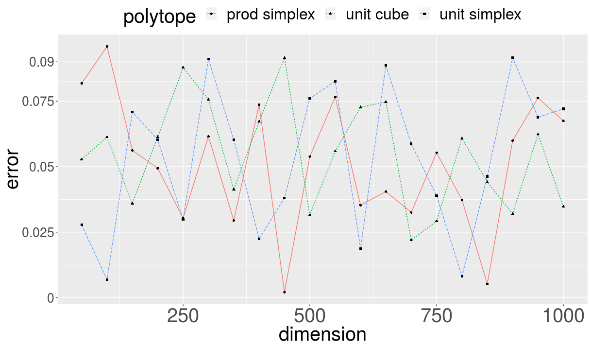
Recall that when we estimate each ratio in Multiphase Monte Carlo (MMC), we have to do an error splitting for the volume ratios that appear in the telescopic product in Equation (7)—i.e. given a requested error for the algorithm compute an error for each volume ratio (see Section 4.3), such that,
We do not split the error equally to all ratios. In particular, we set the requested error for the last ratio to be the smallest ratio in the telescopic product, where is the number of bodies in MMC and the rest errors are set to be equally weighted. The reason is that converges faster than the other ratios in practice. The latter occurs because sampling from is usually faster and more accurate than sampling from any other , e.g. when the body used in MMC is either a ball while is the intersection of with a ball, or an H-polytope while is a Z-polytope.
Then we have to split to the remaining ratios, since . Thus we set so that holds.
In the special case of being a Z-polytope, the body is an H-polytope. We estimate by calling volume using balls in MMC, while the computational time of is a small portion of the total runtime. For the computation of we set the requested error and then we equally split to the ratios respecting .
For the length of the sliding window, we set . Our experiments on the error show this choice offers stability, e.g. in Figure 2 volume always compute a smaller error than the requested error for unit cubes, unit simplices and cross polytopes never exceeds the requested value for .
For each new generated point, we update the average mean and the variance of the sliding window in as follows. Let be the average mean of the ratios in the sliding window, then we write the variance as
We store the sum of the window’s ratios and the sum of the squared ratios . For each new generated point we obtain an updated ratio and the oldest ratio is popped out. We use both the updated and the popped out ratios to update both and and to compute the updated average mean value and st.d. of the current ratios in the sliding window.
In the sequel, we benchmark the proposed algorithm volume tuned as described in the previous sections. We present the result obtained from our experiments for each polytope representation separately.


5.2 Volume experiments for H-polytopes
The implementation of our algorithm, volume, scales up to thousands of dimensions within a few hours. In Tables 2, 3 we report the runtime of volume for cube-, -, --, --, metabolic polytopes and , while volume achieves relative error equal at most . Except of cube-, -, -- we apply the rounding preprocess on Section 3 before volume estimation. Our implementation takes for a few seconds and for a few minutes except for iSDY_1059 that takes almost an hour as it has a larger number of facets (i.e. ). When our implementation takes a few hours, while the runtime increases with the number of facets. However, the runtime for cube- is smaller than the - as the unit simplex has a larger isotropic constant than the unit hypercube; consequently the number of bodies in MMC is larger for the unit simplex. Our implementation is the first one that estimates the volume of very high dimensional Birkhoff polytopes extending the computational results of [24, 17]. In particular, the of order with dimension are computed in hr.
To evaluate the performance of our implementation of volume we count the number of points that billiard_walk generates for the cube-d, -d, rhs-- and . First, for the number of bodies in MMC we notice in Figure 3 that it grows as which agrees with the analysis in Proposition 4. Then, due to the error splitting of Section 5.1.3 the generated points per volume ratio grows as . Thus, the total number of billiard_walk points grows as for those polytopes (left plot in Figures 3). Thus, the total run-time of our implementation grows as , because the per step cost of billiard_walk is .
For the rounding method of Section 3 we experimentally evaluate its quality by counting the number of generated bodies in MMC. In particular, given a skinny polytope we round it and then we compare the number of bodies in MMC with that of isotropic polytopes (e.g. cube-, --). In Figure 3 (right) for rhs-- and we notice that for both rounded and isotropic bodies the number of bodies grows as which is a strong evidence that our rounding method transforms the polytope to a near isotropic position.
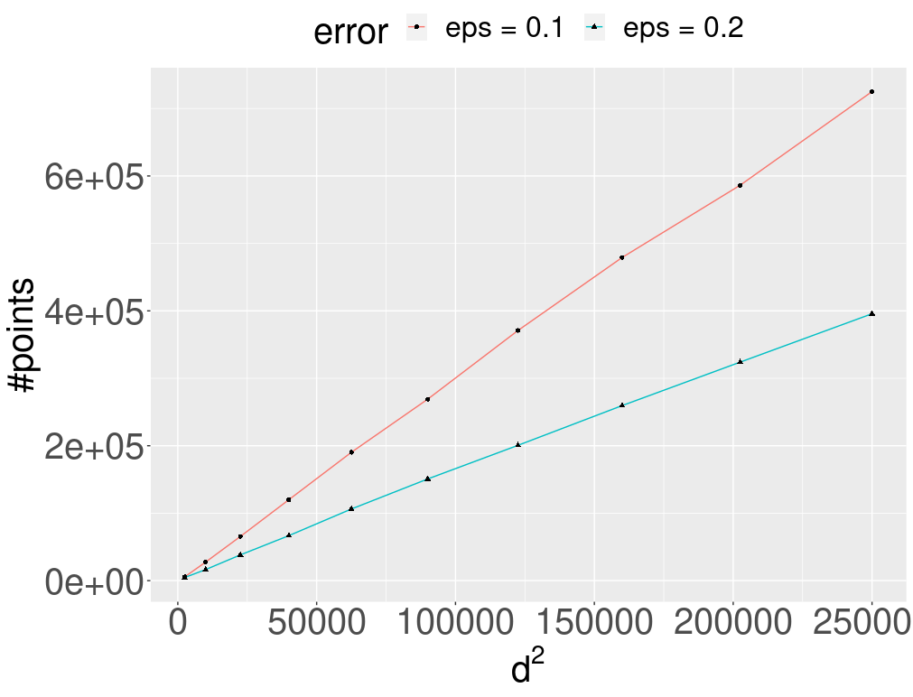

Next, we experimentally study how the complexity of our implementation depends on the input error parameter. In Figure 4 we estimate the volumes of cube- for for two different values for the error parameter . In the left plot we notice that for both values the number of generated points by volume increase as , while a smaller value of just increases the slope of the line, i.e. increases the run-time by a constant. The right plot also confirms this observation; it shows that the run-time of volume increases as for cube-. This is expected as the number of points increases as and the per step cost of billiard_walk is , while for cube-.
Finally we examine the time spend in different steps in the algorithm i.e. rounding, constructing the sequence and volume computation. We conclude that those are highly depended on the convex body. For example for a 100-cube the times for the sequence construction and volume computation is 2.06836 and 4.29843 secs respectively. While for a 100-simplex those numbers are 2.85144 and 17.2575. Intuitively this effect is related to the isotropy of the convex set. Regarding preprocessing/rounding this also depends on the geometry of the body. For example, the rounding of the unit 100-cube takes 0.01427 secs while for a skinny 100-cube takes 6.92041 secs.
5.2.1 Comparison with Cooling Gaussian
We compare our implementation, i.e. volume, against the state-of-the-art MATLAB implementation of CoolingGaussian in [17] for cube-, simplices -d and random polytopes rhs-- with . In Figure 5, we report the total number of generated points for both algorithms to achieve a relative error . CoolingGaussian performs computations up to while volume compute up to in a shorter time frame. More interestingly, the ratio between the number of points generated by CoolingGaussian over the number of points generated by volume increases linearly with the dimension. Then, the comparison of the run-times is determined by the per step cost of the random walks used in each implementation.
The plot in Figure 6 compares the run-times of both implementations for cube-, - in H-representation (left plot), and rhs-- with and . It confirms that volume is faster than CoolingGaussian in [17]. Moreover, notice that the gap on the run-time increases with the dimension as expected. In particular, for our implementation is , and times faster for cube-, - and rhs-- respectively. For our implementation is , and times faster for the same classes of polytopes. For we use polynomial interpolation to estimate the runtime of CoolingGaussian, and our implementation is expected to be around , and times faster for cube-, - and rhs-- respectively.


5.3 Volume experiments for Z-polytopes
Our implementation is the first one that scales up to hundreds of dimensions in order of hours for Z-polytopes. In Table 4 we report the runtimes for both high and low order Z-polytopes. Our implementation, for a -dimensional Z-polytope of order equal to 2 performs reflections (equivalent to boundary oracle calls in [17]) in less than an hour. Considering high order Z-polytopes our implementation scales up to order for and to order and for and respectively in at most half an hour by performing reflections.
The only alternative implementation for Z-polytopes is that in [17], however they estimate volumes only for low dimensional Z-polytopes, while our implementation is undoubtedly superior. Since, we were unable to reproduce the results reported on [17] for Z-polytopes we compare against the data given in [17]. In particular, for a 2-order, -dimensional Z-polytope our implementation performs reflections (boundary oracle calls) in seconds to achieve a relative error smaller than ; the implementation of CoolingGaussian in [17] generates CDHR points which corresponds to boundary oracle calls in seconds to achieve a relative error higher than and smaller than . For a -order, -dimensional Z-polytope our implementation performs reflections in seconds while the CoolingGaussian in [17] performs boundary oracle calls in seconds for the same values of relative errors. Clearly, for those instances, our implementation achieves a better accuracy, while the run-time is at least two order of magnitudes smaller than that of CoolingGaussian in [17].
Exact volume computation of Z-polytopes [28] require an exponential to the dimension number of operations. Thus, it can not scale beyond for low order Z-polytopes.


In the second column of Table 4 we report the type of body we use in MMC. For low order Z-polytopes we use the H-polytope from Section 3 while for high order Z-polytopes we use the unit ball. Our experiments suggest to set the threshold for the order so that the Z-polytope is considered as a low order one. In particular, Figure 8 shows that for order , if we use the H-polytope in MMC, we get a bound on the the number of bodies in MMC for . Note that when we use the H-polytope the number of bodies is smaller for all pairs compared to using the unit ball without applying rounding to the Z-polytope. When we use balls in MMC, decreases for constant as increases. For order equals to the number of balls in MMC, without rounding, is equal or smaller than the number of H-polytopes in MMC when we use the H-polytope of Section 3. Table 4 shows that, for high-order Z-polytopes, , which implies one or two acceptance-rejection steps. Moreover, Table 6 illustrates that the rounding method combined with balls in MMC results to a larger number of bodies in MMC and runtime than the case of using the H-polytope in MMC, while for order equal to the best runtime occurs when using a ball in MMC without rounding. Thus, we use the H-polytope in MMC if the order . We conclude that for a Z-polytope of any order, no rounding preprocessing is needed, if we make the right choice of depending on the order; the maximum number of bodies is for .
To evaluate the efficiency of our implementation for Z-polytopes we wish to count the average number of reflections. We run our implementation of volume for --, -- and -- Z-polytopes. An example for Z-polytopes of order is illustrated in Figure 7. First, as mentioned above our experiments imply that the number of bodies in MMC is for any order for . Moreover, the average number of reflections per point grows sub-linearly in (down-right plot in Figure 7). Considering that billiard_walk generates points per volume ratio, the total number of reflections grows sub-linearly in .


Application: Evaluate Z-polytope approximation
We propose an efficient algorithm for evaluating an over-approximation of a given Z-polytope . Z-polytopes are critical in applications such as autonomous driving [2] or human-robot collaboration [55]. Complexity strongly depends on the order of the encountered Z-polytopes. Thus, a practical solution is to over-approximate , as tight as possible, with another Z-polytope of smaller order. A good measure of the approximation quality (fitness) is
| (16) |
Thus, to compute the approximation quality we need to compute volumes of Z-polytopes. In [41] they compute volumes exactly and deterministically, therefore it is impossible to compute the quality of approximation for .
Here, we exploit our software to test the quality of such approximations. The two methods that are able to scale for are, primarily, the Principal Component Analysis (PCA) and the BOX method from [41]. Both adopt similar approximations and are of comparable reliability; here we focus on PCA: Let and , then is square and generates , where is the “interval hull” from [43]. Over-approximation can be seen as a reduction problem, so that the covariance among the generators of must be null.
Table 4 shows experimental results for Z-polytopes up to and various orders. is obtained exactly by computing one determinant. For PCA over-approximations we show that increases as grows but the same does not occur for fixed as order increases. To our knowledge this is the first time practical volume estimation is used to test approximation methods in that high dimensional spaces.


5.4 Volume experiments for V-polytopes
In Table 5 we report the runtimes of our implementation for several V-polytopes. It estimates volume within a relative error at most in less than an hour. To round a V-polytope, we introduce a new method to control the sandwiching ratio . Since the vertices are known, we put to John’s position [35]. First, we compute the smallest enclosing ellipsoid of ’s vertices by applying the approximation algorithm in [61]. Notice that is also the smallest enclosing ellipsoid of and, if is a ball, then is in John’s position. To round , we apply to it the transformation that maps to the unit ball and repeat until the ratio between ’s longest and shortest axes falls under a given threshold. Our experiments suggest this is much faster than the method in Section 3, as sampling is costly for this representation due to expensive boundary oracle calls. In the left plot of Figure 10, notice that, for rounded V-polytopes, the number of bodies in MMC increases as a linear function of . Moreover, as the number of vertices increases for constant , then decreases. All rounding steps in our experiments for took seconds.
To evaluate the performance of our algorithm we wish to count the average number of reflections (or boundary oracle calls). We run volume for rvc-- and rvs-- polytopes after a rounding step. An example of V-polytopes with number of vertices is illustrated in Figure 9: The average number of reflections grows sublinearly in (down-right plot in Figure 9). The total number of oracle calls grows as (up-left plot in Figure 9). volume performs similarly for both rvc-- and rvs-- polytopes. However, the number of boundary oracle calls decreases as the number of vertices increases for constant . This holds because after a rounding step the more the vertices of a random V-polytope the smaller the sandwiching ratio.
6 Conclusions and future work
We propose a new practical algorithm that computes for the first time volumes of very high-dimensional H-polytopes i.e. in the order of thousands of dimensions and high-dimensional V-, and Z- polytopes i.e. in the order of hundreds of dimensions. We provide strong empirical evidences on the efficiency of the algorithm and its accuracy through extended experiments on benchmark polytopes in computational geometry and bioinformatics.
We expect our software to address hard counting problems, e.g. counting the number of linear extensions of a partially ordered set [60]. Our MMC scheme can be extended for other hard computational problems as Markov Chain Monte Carlo integration for multivariate integrals over a convex polytope. In particular, one could estimate the volume and generate the uniform samples required by one pass. Last but not least, we could exploit parallelism and faster software libraries for linear programs to scale to higher dimensions for V- and Z-polytopes.
References
- [1] Radosław Adamczak, Alexander Litvak, Alain Pajor, and Nicole Tomczak-Jaegermann. Quantitative estimates of the convergence of the empirical covariance matrix in log-concave ensembles. J. of the American Mathematical Society, 23(2):535–561, 2010.
- [2] M. Althoff and J.M. Dolan. Online verification of automated road vehicles using reachability analysis. IEEE Trans. Robotics, 30(4):903–918, 2014.
- [3] Shiri Artstein-Avidan, Haim Kaplan, and Micha Sharir. On radial isotropic position: Theory and algorithms, 2020.
- [4] M. Berkelaar, K. Eikland, and P. Notebaert. lp_solve 5.5, Open source (Mixed-Integer) Linear Programming system, 2004.
- [5] Dimitris Bertsimas and Santosh Vempala. Solving convex programs by random walks. J. ACM, 51(4):540–556, jul 2004.
- [6] Stephen Boyd and Lieven Vandenberghe. Convex Optimization. Cambridge University Press, New York, NY, USA, 2004.
- [7] A. Brieden, P. Gritzmann, R. Kannan, V. Klee, L. Lovász, and M. Simonovits. Approximation of diameters: Randomization doesn’t help. In 39th Symp. Foundations of Computer Science (FOCS), pages 244–251, 1998.
- [8] Andrew Brock, Jeff Donahue, and Karen Simonyan. Large scale GAN training for high fidelity natural image synthesis. In 7th International Conference on Learning Representations, ICLR 2019, New Orleans, LA, USA, May 6-9, 2019. OpenReview.net, 2019.
- [9] B. Büeler and A. Enge. VINCI, 2000. http://www.math.u-bordeaux1.fr/˜aenge/index.php?category=software&page=vinci.
- [10] L. Calès, A. Chalkis, I.Z. Emiris, and V. Fisikopoulos. Practical Volume Computation of Structured Convex Bodies, and an Application to Modeling Portfolio Dependencies and Financial Crises. In Bettina Speckmann and Csaba D. Tóth, editors, 34th International Symposium on Computational Geometry (SoCG 2018), volume 99 of LIPIcs, pages 19:1–19:15, Dagstuhl, Germany, 2018. Schloss Dagstuhl–Leibniz-Zentrum fuer Informatik.
- [11] E. Rodney Canfield and Brendan D. McKay. The asymptotic volume of the birkhoff polytope, 2007.
- [12] Michal Cerný. Goffin’s algorithm for zonotopes. Kybernetika, 48:890–906, 2012.
- [13] Apostolos Chalkis and Vissarion Fisikopoulos. volesti: Volume Approximation and Sampling for Convex Polytopes in R. The R Journal, 13(2):642–660, 2021.
- [14] Apostolos Chalkis, Vissarion Fisikopoulos, Elias Tsigaridas, and Haris Zafeiropoulos. Geometric algorithms for sampling the flux space of metabolic networks. In International Symposium on Computational Geometry, SoCG, LIPIcs. Schloss Dagstuhl - Leibniz-Zentrum für Informatik, 2021. to appear.
- [15] Yuansi Chen. An almost constant lower bound of the isoperimetric coefficient in the kls conjecture. Geom. Funct. Anal., 31:34–61, 2021.
- [16] B. Cousins and S. Vempala. Bypassing KLS: Gaussian cooling and an volume algorithm. In Proc. ACM STOC, pages 539–548, 2015.
- [17] B. Cousins and S. Vempala. A practical volume algorithm. Mathematical Programming Computation, 8, 2016.
- [18] H. Cramer. Mathematical methods of statistics. Princeton University Press, 1946.
- [19] F. Dabbene, P. S. Shcherbakov, and B. T. Polyak. A randomized cutting plane method with probabilistic geometric convergence. SIAM Journal on Optimization, 20(6):3185–3207, 2010.
- [20] L Devroye. Random variate generation for unimodal and monotone densities. Computing, 32(1):43–68, April 1984.
- [21] M. Dyer and A. Frieze. On the complexity of computing the volume of a polyhedron. SIAM Journal on Computing, 17(5):967–974, 1988.
- [22] M. Dyer, A. Frieze, and R. Kannan. A random polynomial-time algorithm for approximating the volume of convex bodies. J. ACM, 38(1):1–17, 1991.
- [23] G. Elekes. A geometric inequality and the complexity of computing volume. Discr. Comput. Geom., 1(4):289–292, 1986.
- [24] I. Z. Emiris and V. Fisikopoulos. Practical polytope volume approximation. ACM Trans. Math. Soft., 44(4):38:1–38:21, 2018. Prelim. version: Proc. SoCG 2014.
- [25] Dani Gamerman and Hedibert F Lopes. Markov chain Monte Carlo: stochastic simulation for Bayesian inference. CRC Press, 2006.
- [26] C. Ge and F. Ma. A fast and practical method to estimate volumes of convex polytopes. In J. Wang and C. Yap, editors, Frontiers in Algorithmics, pages 52–65. Springer, 2015.
- [27] Charles J. Geyer. Markov Chain Monte Carlo Maximum Likelihood. Interface Foundation of North America, 1991. Accepted: 2010-02-24T20:38:06Z.
- [28] E. Gover and N. Krikorian. Determinants and the volumes of parallelotopes and zonotopes. Linear Algebra and its Applications, 413:28–40, 2010.
- [29] Gaël Guennebaud, Benoît Jacob, et al. Eigen v3, 2010.
- [30] S. Haraldsdóttir, B. Cousins, I. Thiele, R.M.T Fleming, and S. Vempala. CHRR: Coordinate Hit-and-run with rounding for uniform sampling of constraint-based models. Bioinformatics, 33(11):1741–1743, 2017.
- [31] Runxin He and Humberto Gonzalez. Numerical synthesis of pontryagin optimal control minimizers using sampling-based methods. In 2017 IEEE 56th Annual Conference on Decision and Control (CDC), pages 733–738. IEEE, 2017.
- [32] Vu Anh Huynh, Sertac Karaman, and Emilio Frazzoli. An incremental sampling-based algorithm for stochastic optimal control. In 2012 IEEE International Conference on Robotics and Automation, pages 2865–2872. IEEE, 2012.
- [33] S. Iyengar. Evaluation of normal probabilities of symmetric regions. SIAM Journal on Scientific and Statistical Computing, 9(3):418–423, 1988.
- [34] H. Jia, A. Laddha, Y.T. Lee, and S.S. Vempala. Reducing isotropy and volume to kls: An volume algorithm, 2020.
- [35] Fritz John. Extremum Problems with Inequalities as Subsidiary Conditions. In Giorgio Giorgi and Tinne Hoff Kjeldsen, editors, Traces and Emergence of Nonlinear Programming, pages 197–215. Springer, Basel, 2014.
- [36] Ian T. Jolliffe and Jorge Cadima. Principal component analysis: a review and recent developments. Philosophical Transactions of the Royal Society A: Mathematical, Physical and Engineering Sciences, 374(2065):20150202, 2016.
- [37] Adam Tauman Kalai and Santosh Vempala. Simulated Annealing for Convex Optimization. Mathematics of Operations Research, 31(2):253–266, 2006. Publisher: INFORMS.
- [38] D.E. Kaufman and R.L. Smith. Direction Choice for Accelerated Convergence in Hit-and-Run Sampling. Operations Research, 46(1):84–95, 1998.
- [39] M. Kerber, R. Tichy, and M.F. Weitzer. Constrained triangulations, volumes of polytopes, and unit equations. In 33rd Intern. Symp. Computational Geometry (SoCG 2017), pages 46:1–46:15, Germany, 2017. Schloss Dagstuhl - Leibniz-Zentrum für Informatik.
- [40] Yunbum Kook, Yin Tat Lee, Ruoqi Shen, and Santosh S. Vempala. Sampling with riemannian hamiltonian monte carlo in a constrained space. CoRR, abs/2202.01908, 2022.
- [41] A.K. Kopetzki, B. Schürmann, and M. Althoff. Methods for order reduction of zonotopes. In Proc. IEEE Annual Conf. Decision & Control (CDC), pages 5626–5633, 2017.
- [42] D. Kraft. A software package for sequential quadratic programming. Technical report, DFVLR-FB 88-28, Institut für Dynamik der Flugsysteme, 1988.
- [43] W. Kühn. Rigorously computed orbits of dynamical systems without the wrapping effect. Computing, 61:47–67, 1998.
- [44] Aditi Laddha and Santosh Vempala. Convergence of Gibbs Sampling: Coordinate Hit-and-Run Mixes Fast, 2020.
- [45] Y.T. Lee and S.S. Vempala. Convergence rate of riemannian hamiltonian monte carlo and faster polytope volume computation. In Proceedings of the 50th Annual ACM SIGACT Symposium on Theory of Computing, STOC 2018, page 1115–1121, New York, NY, USA, 2018. Association for Computing Machinery.
- [46] L. Lovász, R. Kannan, and M. Simonovits. Random walks and an volume algorithm for convex bodies. Random Structures and Algorithms, 11:1–50, 1997.
- [47] L. Lovász and S. Vempala. Hit-and-run from a corner. SIAM J. Comp., 35(4):985–1005, 2006.
- [48] L. Lovász and S. Vempala. Simulated annealing in convex bodies and an O volume algorithms. J. Computer & System Sciences, 72:392–417, 2006.
- [49] O. Mangoubi and N. K. Vishnoi. Faster polytope rounding, sampling, and volume computation via a sub-linear ball walk. In 2019 IEEE 60th Annual Symposium on Foundations of Computer Science (FOCS), pages 1338–1357, 2019.
- [50] L. Martino, V. Elvira, D. Luengo, J. Corander, and F. Louzada. Orthogonal parallel mcmc methods for sampling and optimization. Digital Signal Processing, 58:64–84, Nov 2016.
- [51] Luca Martino, David Luengo, and Joaquín Míguez. Independent Sampling for Multivariate Densities. In Luca Martino, David Luengo, and Joaquín Míguez, editors, Independent Random Sampling Methods, Statistics and Computing, pages 197–247. Springer International Publishing, Cham, 2018.
- [52] K.G. Murty. Ball centers of special polytopes. Technical report, Department of Industrial & Operations Engineering, University of Michigan, 2009.
- [53] Hariharan Narayanan and Piyush Srivastava. On the mixing time of coordinate hit-and-run, 2020.
- [54] Radford M Neal et al. MCMC using Hamiltonian dynamics. Handbook of markov chain monte carlo, 2(11):2, 2011.
- [55] A. Pereira and M. Althoff. Safety control of robots under computed torque control using reachable sets. In Proc. IEEE Inter. Conf. Robotics Automation (ICRA), pages 331–338, 2015.
- [56] B.T. Polyak and E.N. Gryazina. Billiard walk - a new sampling algorithm for control and optimization. IFAC Proceedings Volumes, 47(3):6123–6128, 2014. 19th IFAC World Congress.
- [57] Chaitra Sarathy, Martina Kutmon, Michael Lenz, Michiel E. Adriaens, Chris T. Evelo, and Ilja C.W. Arts. Efmviz: A cobra toolbox extension to visualize elementary flux modes in genome-scale metabolic models. Metabolites, 10(2), 2020.
- [58] J. Schellenberger and B.O. Palsson. Use of randomized sampling for analysis of metabolic networks. J. Biological Chemistry, 284(9):5457–5461, 2009.
- [59] M. Schumer and K. Steiglitz. Adaptive step size random search. IEEE Transactions on Automatic Control, 13(3):270–276, June 1968. Conference Name: IEEE Transactions on Automatic Control.
- [60] T. Talvitie, K. Kangas, T. Niinimäki, and M. Koivisto. Counting linear extensions in practice: Mcmc versus exponential monte carlo. In AAAI Conference on Artificial Intelligence, 2018.
- [61] Michael J. Todd and E. Alper Yildirim. On Khachiyan’s algorithm for the computation of minimum-volume enclosing ellipsoids. Discrete Applied Mathematics, 155(13):1731–1744, 2007.
- [62] A. Venzke, D.K. Molzahn, and S. Chatzivasileiadis. Efficient creation of datasets for data-driven power system applications. Electric Power Systems Research, 190:106614, 2021.
- [63] Frederick Wong, Christopher K. Carter, and Robert Kohn. Efficient estimation of covariance selection models. Biometrika, 90(4):809–830, 2003.
Appendix A Figures and tables
| H-polytope | volume | std/mean | error | points | time | |
| cross- | 2.81e-04 | 0.06 | 0.01 | 1.0 | 1.50e+03 | 0.11 |
| cross- | 1.30e-06 | 0.07 | 0.01 | 1.0 | 1.50e+03 | 1.17 |
| cross- | 2.49e-08 | 0.04 | 0.01 | 1.0 | 1.50e+03 | 12.8 |
| cube- | 1.18e+30 | 0.15 | 0.07 | 9.2 | 2.80e+04 | 1.5 |
| cube- | 1.96e+75 | 0.16 | 0.08 | 34.5 | 1.96e+05 | 36.2 |
| cube- | 3.38e+150 | 0.25 | 0.03 | 84.7 | 7.09e+05 | 425 |
| cube- | 5.75e+225 | 0.22 | 0.03 | 139.9 | 1.52e+06 | 1501 |
| cube- | 2.11e+301 | 0.29 | 0.03 | 201.0 | 2.70e+06 | 6180 |
| - | 1.02e-158 | 0.16 | 0.05 | 21.0 | 1.01e+05 | 4.8 |
| - | 3.20e-493 | 0.15 | 0.03 | 66.3 | 5.05e+05 | 66.4 |
| - | 7.55e-1135 | 0.20 | 0.08 | 149.1 | 1.65e+06 | 847.8 |
| - | 3.70e-1833 | 0.17 | 0.04 | 237.9 | 3.28e+06 | |
| - | 2.67e-2568 | 0.24 | 0.07 | 328.4 | 5.34e+06 | |
| -- | 1.07e-129 | 0.21 | 0.01 | 22.3 | 9.90e+04 | 3.3 |
| -- | 2.91e-419 | 0.18 | 0.03 | 67.0 | 5.07e+05 | 107.2 |
| -- | 9.10e-986 | 0.23 | 0.05 | 151.3 | 1.69e+06 | 958.5 |
| -- | 6.26e-1609 | 0.21 | 0.06 | 239.3 | 3.35e+06 | |
| -- | 6.22e-2269 | 0.24 | 0.07 | 332.5 | 5.39e+06 | |
| -- | 4.19e-46 | 0.11 | ?? | 10.6 | 3.33e+04 | 5.25 |
| -- | 2.75e-205 | 0.20 | ?? | 50.0 | 3.22e+05 | 253 |
| -- | 4.18e+275 | 0.23 | ?? | 202.1 | 2.61e+06 | |
| -- | 1.47e+216 | 0.21 | ?? | 172.3 | 1.90e+06 | |
| e_coli_core [174-24] | 3.37e-47 | 0.08 | ?? | 2.0 | 3.52e+03 | 0.16 |
| iAB_RBC_283 [906-130] | 1.73e+43 | 0.28 | ?? | 23.9 | 1.11e+05 | 31.3 |
| iJR904 [1132-227] | 6.00e+53 | 0.25 | ?? | 50.8 | 3.38e+05 | 169.3 |
| iAT_PLT_636 [2016-289] | 3.65e-854 | 0.25 | ?? | 66.3 | 4.99e+05 | 512.7 |
| iSDY_1059 [2966-509] | 2.25e-350 | 0.27 | ?? | 136.0 | 1.43e+06 | 3486 |
| Recon1 [4934-931] | 8.01e-5321 | 0.17 | ?? | 266.1 | 3.84e+06 |
| exact | asymptotic | volume | error | std/mean | points | time | |||
| 4 | 1.12 | 1.410849 | 1.12e+00 | 0.00 | 0.02 | 1 | 1.50e+03 | 0.01 | |
| 9 | 6.21e-02 | 7.61e-02 | 6.17e-02 | 0.01 | 0.02 | 1 | 1.50e+03 | 0.01 | |
| 16 | 1.41e-04 | 1.69e-04 | 1.38e-04 | 0.02 | 0.01 | 1 | 1.52e+03 | 0.03 | |
| 25 | 7.35e-09 | 8.62e-09 | 7.35e-09 | 0.00 | 0.05 | 2.3 | 3.63e+03 | 0.06 | |
| 36 | 5.64e-15 | 6.51e-15 | 5.49e-15 | 0.03 | 0.02 | 4.0 | 7.98e+03 | 0.16 | |
| 49 | 4.42e-23 | 5.03e-23 | 4.24e-23 | 0.04 | 0.05 | 6.4 | 1.62e+04 | 0.37 | |
| 64 | 2.60e-33 | 2.93e-33 | 2.54e-33 | 0.02 | 0.03 | 9.2 | 2.82e+04 | 0.86 | |
| 81 | 8.78e-46 | 9.81e-46 | 8.46e-46 | 0.04 | 0.05 | 13.1 | 4.69e+04 | 1.9 | |
| 100 | ?? | 1.49e-60 | 1.24e-60 | ?? | 0.05 | 17.6 | 7.17e+04 | 3.5 | |
| 121 | ?? | 8.38e-78 | 7.28e-78 | ?? | 0.10 | 23.1 | 1.07e+05 | 6.7 | |
| 144 | ?? | 1.43e-97 | 1.205e-97 | ?? | 0.19 | 29.2 | 1.49e+05 | 11.9 | |
| 169 | ?? | 6.24e-120 | 5.13e-120 | ?? | 0.08 | 35.9 | 2.04e+05 | 20.7 | |
| 196 | ?? | 5.94e-145 | 4.92e-145 | ?? | 0.05 | 43.4 | 2.68e+05 | 34.5 | |
| 225 | ?? | 1.06e-172 | 9.62e-173 | ?? | 0.12 | 51.9 | 3.49e+05 | 56.3 | |
| 256 | ?? | 3.10e-203 | 2.50e-203 | ?? | 0.10 | 60.9 | 4.41e+05 | 84.2 | |
| 289 | ?? | 1.30e-236 | 1.03e-237 | ?? | 0.10 | 72.0 | 5.65e+05 | 129 | |
| 324 | ?? | 6.96e-273 | 5.41e-273 | ?? | 0.09 | 82.0 | 6.88e+05 | 198 | |
| 361 | ?? | 4.23e-312 | 3.31e-312 | ?? | 0.11 | 94.9 | 8.46e+05 | 297 | |
| 400 | ?? | 2.62e-354 | 1.77e-354 | ?? | 0.27 | 101.6 | 9.40e+05 | 325 | |
| 441 | ?? | 1.49e-399 | 1.49e-399 | ?? | 0.17 | 115.0 | 1.12e+06 | 453 | |
| 484 | ?? | 7.10e-448 | 4.33e-448 | ?? | 0.30 | 128.8 | 1.33e+06 | 624 | |
| 529 | ?? | 2.57e-499 | 2.10e-499 | ?? | 0.27 | 143.7 | 1.55e+06 | 845 | |
| 576 | ?? | 6.46e-554 | 5.56e-554 | ?? | 0.28 | 158.8 | 1.82e+06 | 1060 | |
| 625 | ?? | 1.04e-611 | 7.80e-612 | ?? | 0.22 | 176.3 | 2.11e+06 | 1405 | |
| 676 | ?? | 9.81e-673 | 1.00e-672 | ?? | 0.30 | 194.0 | 2.41e+06 | 1918 | |
| 729 | ?? | 5.05e-737 | 6.13e-737 | ?? | 0.31 | 211.1 | 2.75e+06 | 2573 | |
| 784 | ?? | 1.31e-804 | 1.17e-804 | ?? | 0.31 | 231.5 | 3.15e+06 | 3539 | |
| 841 | ?? | 1.60e-875 | 1.35e-875 | ?? | 0.35 | 249.1 | 3.53e+06 | 4982 | |
| 900 | ?? | 8.55e-950 | 8.43e-950 | ?? | 0.40 | 272.9 | 4.02e+06 | 6967 | |
| 961 | ?? | 1.86e-1027 | 1.58e-1027 | ?? | 0.39 | 293.8 | 4.47e+06 | 8905 | |
| 1024 | ?? | 1.56e-1108 | 1.37e-1108 | ?? | 0.42 | 314.1 | 4.97e+06 | 11105 |
| Z-polytope | Body | order | volume | std/mean | Refl | time | |||
|---|---|---|---|---|---|---|---|---|---|
| -- | Ball | 5.47e+34 | 0.06 | 1 | 3.15e+03 | 13 | 2.24e+37 | 1.82 | |
| -- | Ball | 3.19e+38 | 0.07 | 1 | 3.00e+03 | 50 | 1.42e+41 | 1.84 | |
| -- | Ball | 2.57e+41 | 0.04 | 1 | 2.95e+03 | 180 | 1.08e+44 | 1.83 | |
| -- | Ball | 1.85e+43 | 0.05 | 1 | 2.88e+03 | 320 | 7.30e+45 | 1.82 | |
| -- | Ball | 3.79e+51 | 0.07 | 1 | 4.34e+03 | 50 | 3.63e+56 | 2.15 | |
| -- | Ball | 8.14e+57 | 0.05 | 1 | 3.39e+03 | 183 | 7.84e+62 | 2.15 | |
| -- | Ball | 3.45e+62 | 0.07 | 1 | 3.22e+03 | 503 | 3.20e+62 | 2.14 | |
| -- | Ball | 1.47e+65 | 0.05 | 1 | 3.14e+03 | 1071 | 1.31e+70 | 2.14 | |
| -- | Ball | 1.31e+67 | 0.09 | 1 | 4.53e+03 | 72 | 7.91e+74 | 2.45 | |
| -- | Ball | 5.58e+69 | 0.05 | 1 | 4.46e+03 | 110 | 2.90e+77 | 2.43 | |
| -- | Ball | 1.12e+77 | 0.05 | 1 | 3.76e+03 | 455 | 4.91e+84 | 2.41 | |
| -- | Ball | 1.93e+83 | 0.06 | 1 | 3.51e+03 | 1736 | 7.56e+90 | 2.40 | |
| -- | Ball | 8.15e+99 | 0.10 | 1 | 5.45e+03 | 280 | 5.73e+113 | 2.89 | |
| -- | Ball | 1.49e+104 | 0.06 | 1 | 5.46e+03 | 503 | 1.04e+118 | 2.89 | |
| -- | Hpoly | 1.3 | 1.47e+16 | 0.07 | 1 | 7.26e+04 | 357 | 9.25e+54 | 4.43 |
| -- | Hpoly | 1.3 | 6.39e+08 | 0.08 | 3.0 | 1.37e+05 | 1604 | 5.03e+71 | 6.11 |
| -- | Hpoly | 1.3 | 4.73e+17 | 0.05 | 3.0 | 1.97e+05 | 2851 | 1.01e+101 | 6.81 |
| -- | Hpoly | 1.5 | 9.24e+19 | 0.07 | 1 | 5.68e+04 | 332 | 1.04e+58 | 4.31 |
| -- | Hpoly | 1.5 | 3.46e+21 | 0.05 | 2.7 | 7.28e+04 | 901 | 9.70e+75 | 4.79 |
| -- | Hpoly | 1.5 | 5.30e+37 | 0.09 | 3 | 1.27e+05 | 2647 | 2.66e+108 | 5.09 |
| -- | Hpoly | 1.7 | 2.06e+132 | 0.07 | 2 | 4.18e+04 | 329 | 2.65e+175 | 5.23 |
| -- | Hpoly | 1.7 | 1.74e+176 | 0.10 | 2.8 | 5.17e+04 | 857 | 2.63e+237 | 5.81 |
| -- | Hpoly | 1.7 | 3.74e+222 | 0.14 | 3 | 8.06e+04 | 2402 | 1.98e+303 | 6.42 |
| -- | Hpoly | 2 | 1.85e+135 | 0.12 | 2 | 3.38e+04 | 337 | 1.89e+177 | 5.01 |
| -- | Hpoly | 2 | 2.27e+186 | 0.15 | 2.6 | 5.72+04 | 1227 | 2.56e+245 | 5.47 |
| -- | Hpoly | 2 | 5.86e+231 | 0.17 | 3 | 6.37e+04 | 2652 | 1.85e+310 | 6.10 |
| -- | Hpoly | 3 | 2.95e+155 | 0.21 | 2 | 1.98e+04 | 417 | 6.61e+191 | 4.03 |
| -- | Hpoly | 3 | 5.59e+206 | 0.19 | 2.8 | 2.97e+04 | 2497 | 9.47e+260 | 4.76 |
| V-polytope | volume | std/mean | Refl | error | time | exact time | |
|---|---|---|---|---|---|---|---|
| cross- | 4.546e-13 | 0.05 | 1.0 | 10.9e+03 | 0.05 | 3 | |
| cross- | 1.43e-128 | 0.05 | 2.0 | 5.80e+04 | 0.08 | 112 | |
| cross- | 1.50e-64 | 0.07 | 2.0 | 2.99e+04 | 0.08 | 24 | |
| cross- | 1.65e-95 | 0.10 | 3.0 | 3.92e+04 | 0.02 | 53 | |
| - | 1.17e-48 | 0.15 | 6.1 | 2.42e+05 | 0.05 | 230 | 0.008 |
| - | 1.12e-82 | 0.14 | 11.2 | 5.13e+05 | 0.07 | 989 | 0.02 |
| - | 1.35e-119 | 0.21 | 15.6 | 1.21e+06 | 0.03 | 4140 | 0.07 |
| cube- | 1052.4 | 0.07 | 1 | 1.50e+03 | 0.03 | 54 | |
| cube- | 1930.2 | 0.06 | 1 | 1.5e+03 | 0.06 | 155 | |
| cube- | 4240.6 | 0.08 | 1 | 1.81e+03 | 0.04 | 567 | |
| cube- | 7538.2 | 0.06 | 1 | 1.87e+03 | 0.08 | 2937 | |
| - | 2.43e-62 | 0.10 | 1.0 | 4.08e+04 | ?? | 178 | |
| - | 2.05e-77 | 0.12 | 1.0 | 4.78e+04 | ?? | 298 | |
| - | 3.62e-93 | 0.14 | 1.0 | 5.43e+04 | ?? | 466 | |
| - | 1.72e-109 | 0.08 | 1.9 | 7.32e+04 | ?? | 756 | |
| - | 3.16e-126 | 0.12 | 2.0 | 7.79e+04 | ?? | 1066 | |
| -- | 1.35e-01 | 0.07 | 1.0 | 1.22e+04 | 0.02 | 35.4 | |
| -- | 8.98e-03 | 0.05 | 1.0 | 1.49e+04 | 0.00 | 358 | |
| -- | 1.04e-01 | 0.08 | 1.0 | 1.63e+04 | 0.00 | 403 | |
| -- | 1.43e-02 | 0.07 | 1.0 | 1.74e+04 | 0.02 | 321 | |
| - | 2.31 | 0.07 | 1.0 | 9.24e+03 | 0.00 | 3.1 | 0.02 |
| - | 1.40 | 0.06 | 1.0 | 1.28e+04 | 0.04 | 8.8 | 44.6 |
| - | 5.21e-01 | 0.06 | 1.0 | 1.67e+04 | ?? | 29.5 | |
| -- | 1.77e-03 | 0.04 | 1.0 | 8.79e+03 | 0.02 | 6.9 | 0.03 |
| -- | 2.75e+01 | 0.06 | 1.0 | 7.60e+03 | 0.00 | 7.2 | 0.07 |
| -- | 1.36e+04 | 0.05 | 1.0 | 7.38e+03 | 0.02 | 9.3 | 0.5 |
| -- | 1.40e+06 | 0.07 | 1.0 | 7.22e+03 | 0.01 | 14.1 | 2.4 |
| rvs-- | 1.51e-05 | 0.07 | 1 | 1.11e+04 | 0.06 | 3.2 | 0.01 |
| rvc-- | 5.30e-02 | 0.05 | 1 | 9.65e+03 | 0.05 | 4.5 | 0.09 |
| rvs-- | 3.85e-04 | 0.09 | 1 | 7.19e+03 | 0.05 | 4.8 | 0.4 |
| rvc-- | 0.440 | 0.05 | 1 | 7.27e+03 | 0.02 | 3.7 | 0.9 |
| rvs-- | 1.01e-03 | 0.07 | 1 | 9.34e+03 | 0.04 | 6.2 | 87 |
| rvc-- | 8.72e-04 | 0.05 | 1 | 8.98e+03 | 0.02 | 9.1 | 549 |
| rvs-- | 2.86e-10 | 0.06 | 1 | 1.23e+04 | ?? | 7.7 | |
| rvc-- | 1.04e-18 | 0.08 | 1 | 2.25e+03 | ?? | 215 | |
| rvc-- | 1.48e-39 | 0.10 | 3.1 | 5.18e+04 | ?? | 267 | |
| rvc-- | 5.94e-57 | 0.08 | 4.5 | 7.88e+04 | ?? | 763 | |
| rvc-- | 1.31e-75 | 0.07 | 5.8 | 1.00e+05 | ?? | 2237 | |
| rvs-- | 2.04e-72 | 0.11 | 2.2 | 5.39e+04 | ?? | 422 | |
| rvs-- | 5.17e-106 | 0.19 | 3.0 | 7.50e+04 | ?? | 1069 | |
| rvs-- | 9.13e-142 | 0.13 | 4.1 | 1.05e+05 | ?? | 2520 | |
| rvc-- | 2.72e-33 | 0.14 | 2.1 | 5.25e+04 | ?? | 354 | |
| rvc-- | 5.52e-49 | 0.15 | 3.0 | 7.93e+04 | ?? | 1052 | |
| rvc-- | 1.04e-65 | 0.16 | 4.0 | 1.04e+05 | ?? | 2278 |
| no rounding ( is a ball) | rounding | H-polytope approx. | |||||||
| Z-polytope | Refl | time | Refl | time | Refl | time | |||
| -- | 3 | 3.09e+04 | 54 | 1 | 2.80e+04 | 50 | 1 | 1.57e+04 | 35.9 |
| -- | 4 | 4.23e+04 | 126 | 1 | 3.89e+04 | 115 | 1 | 1.71e+04 | 67.1 |
| -- | 5 | 5.53e+04 | 282 | 1 | 5.10e+04 | 270 | 1 | 1.84e+04 | 133 |
| -- | 7 | 9.04e+04 | 825 | 1 | 6.61e+04 | 575 | 2 | 3.52e+04 | 369 |
| -- | 1 | 7.01e+03 | 57 | 1 | 1.61e+04 | 111 | 1 | 7.24e+03 | 64 |
| -- | 1 | 7.79e+03 | 126 | 1 | 2.07e+04 | 323 | 1 | 7.81e+03 | 163 |
| -- | 1 | 8.33e+03 | 319 | 1 | 2.67e+04 | 858 | 2 | 1.24e+04 | 414 |
| -- | 1 | 9.53e+03 | 721 | 1 | 3.35e+04 | 2121 | 2 | 1.37e+04 | 1168 |

Appendix B Software tutorial
This section aims in providing a brief outline on how to reproduce the computational results of this article. First, to run the C++ implementation of volume we suggest to use the R interface. To install the R interface follow the instructions given at the repository:
https://github.com/GeomScale/volume_approximation/blob/v1.1.3/doc/r_interface.md
After installation the user should open an R terminal or alternatively use Rstudio and load the volesti package running:
Then we start using the package by illustrating polytope generators that could be used to generate polytopes in various representations.
Note that when the value of the input flag of generator in the gen_rand_zonotope() is ’uniform’ then the function generates a random --. Other options are ’gaussian’ for random -- and ’exponential’ for random --.
To estimate the volume of a polytope with our implementation of volume the user should use the function volume(). The output contains both the estimated volume and its logarithm (useful in overflow or underflow cases).
To request polytope rounding before volume estimation using the methods we introduced in Section 3 run:
To estimate the volume with algorithm CoolingGaussian as described in [17],
To compute the PCA over-approximation of a Z-polytope,