QPS-r: A Cost-Effective Iterative Switching Algorithm for Input-Queued Switches
Abstract
In an input-queued switch, a crossbar schedule, or a matching between the input ports and the output ports needs to be computed in each switching cycle, or time slot. Designing switching algorithms with very low computational complexity, that lead to high throughput and small delay is a challenging problem. There appears to be a fundamental tradeoff between the computational complexity of the switching algorithm and the resultants throughput and delay. Parallel maximal matching algorithms (adapted for switching) appear to have stricken a sweet spot in this tradeoff, and prior work has shown the following performance guarantees. Using maximal matchings in every time slot results in at least 50% switch throughput and order-optimal (i.e., independent of the switch size ) average delay bounds for various traffic arrival processes. On the other hand, their computational complexity can be as low as per port/processor, which is much lower than those of the algorithms such as maximum weighted matching which ensures better throughput performance.
In this work, we propose QPS-r, a parallel iterative switching algorithm that has the lowest possible computational complexity: per port. Using Lyapunov stability analysis, we show that the throughput and delay performance is identical to that of maximal matching algorithm. Although QPS-r builds upon an existing technique called Queue-Proportional Sampling (QPS), in this paper, we provide analytical guarantees on its throughput and delay under i.i.d. traffic as well as a Markovian traffic model which can model many realistic traffic patterns. We also demonstrate that QPS-3 (running 3 iterations) has comparable empirical throughput and delay performances as iSLIP (running iterations), a refined and optimized representative maximal matching algorithm adapted for switching.
Keywords:
Crossbar scheduling; input-queued switch; Lyapunov stability analysis1 Introduction
The volume of network traffic across the Internet and in data-centers continues to grow relentlessly, thanks to existing and emerging data-intensive applications, such as big data analytics, cloud computing, and video streaming. At the same time, the number of network-connected devices is exploding, fueled by the wide adoption of smart phones and the emergence of the Internet of things. To transport and “direct" this massive amount of traffic to their respective destinations, switches and routers capable of connecting a large number of ports (called high-radix [1, 2]) and operating at very high line rates are badly needed.
Many present day high-performance switching systems in Internet routers and data-center switches employ an input-queued crossbar to interconnect their input ports and output ports. In an input-queued crossbar switch, each input port can be connected to only one output port and vice versa in each switching cycle or time slot. Hence, in every time slot, the switch needs to compute a one-to-one matching between input and output ports (i.e., the crossbar schedule). A major research challenge in designing high-link-rate high-radix switches is to develop algorithms that can compute “high quality” matchings – i.e., those that result in high switch throughput and low queueing delays for packets – in a few nanoseconds. Clearly, a suitable switching algorithm has to have very low computational complexity, yet output “fairly good” matching decisions most of time.
1.1 The Family of Maximal Matchings
A family of parallel iterative algorithms for computing maximal matching (one to which no edge can be added for it to remain a matching, a definition that will be made precise in Section 2) are arguably the best candidates for switching in high-link-rate high-radix switches, because they have reasonably low computational complexities, yet can provide fairly good throughput and delay performance guarantees. More specifically, using maximal matchings as crossbar schedules results in at least 50% switch throughput in theory (and usually much higher throughput in practice) [3]. In addition, it results in low packet delays that also have excellent scaling behaviors such as order-optimal (i.e., independent of switch size ) under various traffic arriving processes when the offered load is less than 50% (i.e., within the provable stability region) [4]. In comparison, matchings of higher qualities such as maximum matching (with the largest possible number of edges) and maximum weighted matching (with the highest total edge weight) are much more expensive to compute. Hence, it is fair to say that, maximal matching algorithms overall deliver the biggest “bang” (performance) for the “buck” (computational complexity).
Unfortunately, parallel maximal matching algorithms are still not “dirt cheap” computationally. More specifically, all existing parallel algorithms that compute maximal matchings on general bipartite graphs require a minimum of iterations (rounds of message exchanges). This minimum is attained by the classical algorithm of Israel and Itai [5]; the PIM algorithm [6] is a slight adaptation of this classical algorithm to the switching context, and iSLIP [7] further improves upon PIM by reducing its per-iteration per-port computational complexity to via de-randomizing a computationally expensive ( complexity to be exact) operation in PIM.
1.2 QPS-r: Bigger Bang for the Buck
In this work, we propose QPS-r, a parallel iterative switching algorithm that has the lowest possible computational complexity: per port. More specifically, QPS-r requires only (a small constant independent of ) iterations to compute a matching, and the computational complexity of each iteration is only ; here QPS stands for Queue-Proportional Sampling, an add-on technique proposed in [8] that we will describe shortly. Yet, even the matchings that QPS-1 (running only a single iteration) computes have the same (reasonably high) quality as maximal matchings in the following sense: Using such matchings as crossbar schedules results in exactly the same aforementioned provable throughput and delay guarantees as using maximal matchings, as we will show using Lyapunov stability analysis. QPS-r performs as well as maximal matching algorithms not just in theory: We will show in Section 6 that QPS-3 (running 3 iterations) has comparable empirical throughput and delay performances as iSLIP (running iterations), a refined and optimized representative maximal matching algorithm adapted for switching, under various workloads. Note that matchings that QPS-r computes are generally not maximal. QPS-r can make do with less (iterations) because the queue-proportional sampling operation implicitly makes use of the queue (VOQ) length information, which maximal matching algorithms do not. One major contribution of this work is to discover the family of (QPS-r)-generated matchings that is even more cost-effective.
Although QPS-r builds on the QPS data structure and algorithm proposed in [8], our work on QPS-r is very different in three important aspects. First, in [8], QPS was used only as an add-on to other switching algorithms such as iSLIP [7] and SERENA [9] by generating a starter matching for other switching algorithms to further refine, whereas in this work, QPS-r is used only as a stand-alone algorithm. Second, we are the first to discover and prove that (QPS-r)-generated matchings and maximal matchings provide exactly the same aforementioned performance guarantees, whereas in [8], no such mathematical similarity or connection was mentioned. Third, the establishment of this mathematical similarity is an important theoretical contribution in itself, because maximal matchings have long been established as a cost-effective family both in switching [6, 7] and in wireless networking [4, 10], and with this connection we have considerably enlarged this family.
Although we show that QPS-r has exactly the same throughput and delay bounds as those of maximal matchings established in [3, 4, 10], our proofs are different for the following reason. A departure inequality (see Property 1), satisfied by all maximal matching algorithms was used in the throughput analysis of [3] and the delay analysis of [4, 10]. This inequality, however, is not satisfied by QPS-r in general. Instead, QPS-r satisfies this departure inequality in expectation, which is a much weaker guarantee. The methodological contributions of this work are twofold. First, we prove two theorems stating that this much weaker guarantee is sufficient for obtaining the same throughput and delay bounds under i.i.d. traffic arrivals. Second, we generalize both results to the more general Markovian arrivals.
The rest of this paper is organized as follows. In Section 2, we provide some background on the switching problem in input-queued crossbar switches. In Section 3, we first review QPS, and then describe QPS-r. Then in Sections 4 and 5, we derive the throughput and the queue length (and delay) bounds of QPS-r, followed by the performance evaluation in Section 6. In Section 7, we survey related work before concluding this paper in Section 8.
2 Background on Crossbar Scheduling
In this section, we provide a brief introduction to the crossbar scheduling (switching) problem, and describe and compare the aforementioned three different types of matchings. Throughout this paper we adopt the standard assumption [11, Chapter 2, Page 21] that all the incoming variable-length packets are first segmented into fixed-length packets (also referred to as cells), and then reassembled at their respective output ports before leaving the switch. Each fixed-length packet takes one time slot to switch. We also assume that all input links/ports and output links/ports operate at the same normalized line rate of , and so do all wires and crosspoints inside the crossbar.
2.1 Input-Queued Crossbar Switch
In an input-queued crossbar switch, each input port has Virtual Output Queues (VOQs) [12]. The VOQ at input port serves as a buffer for packets going from input port to output port . The use of VOQs solves the Head-of-Line (HOL) blocking issue [13], which severely limits the throughput of the switch system.
An input-queued crossbar can be modeled as a bipartite graph, of which the two disjoint vertex sets are the input ports and the output ports respectively. In this bipartite graph, there is an edge between input port and output port , if and only if the VOQ at input port , the corresponding VOQ, is nonempty. The weight of this edge is defined as the length of (i.e., the number of packets buffered at) this VOQ. A set of such edges constitutes a valid crossbar schedule, or a matching, if any two of them do not share a common vertex. The weight of a matching is the total weight of all the edges belonging to it (i.e., the total length of all corresponding VOQs).
A matching can be represented as an sub-permutation matrix (a - matrix that contains at most one entry of “” in each row and in each column) as follows: if and only if the edge between input port and output port is contained in (i.e., input port is matched to output port in ). To avoid any confusion, only (not ) is used to denote a matching in the sequel, and it can be both a set (of edges) and a matrix.
2.2 Maximal Matching
As mentioned in Section 1, three types of matchings play important roles in crossbar scheduling problems: (I) maximal matchings, (II) maximum matchings, and (III) maximum weighted matchings. A matching is called a maximal matching, if it is no longer a matching, when any edge not in is added to it. A matching with the largest possible number of edges is called a maximum matching or maximum cardinality matching. Neither maximal matchings nor maximum matchings take into account the weights of edges, whereas maximum weighted matchings do. A maximum weighted matching is one that has the largest total weight among all matchings. By definition, any maximum matching or maximum weighted matching is also a maximal matching, but neither converse is generally true.
As mentioned earlier, the family of maximal matchings has long been recognized as a cost-effective family for crossbar scheduling. Compared to maximal matching, maximum weighted matching (MWM) (i.e., the well-known MaxWeight scheduler [14] in the context of scheduling transmissions in wireless networking) is much less cost effective. Although MWM provides stronger provable guarantees such as % switch throughput [15, 16] and average packet delay [17] whenever the offered load is less than 100% in theory (and usually much better empirical delay performance in practice as shown in [15]), the state-of-the-art serial MWM algorithm (suitable for switching) has a prohibitively high computational complexity of [18], where is the maximum possible weight (length) of an edge (VOQ). By the same measure, maximum matching is not a great deal either: It is only slightly cheaper to compute than MWM, yet using maximum matchings as crossbar schedules generally cannot guarantee 100% throughput [19].
3 The QPS- Algorithm
The QPS-r algorithm simply runs iterations of QPS (Queue-Proportional Sampling) [8] to arrive at a matching, so its computational complexity per port is exactly times those of QPS. Since is a small constant, it is , same as that of QPS. In the following two subsections, we describe QPS and QPS-r respectively in more details.
3.1 Queue-Proportional Sampling (QPS)
QPS was used in [8] as an “add-on” to augment other switching algorithms as follows. It generates a starter matching, which is then populated (i.e., adding more edges to it) and refined, by other switching algorithms such as iSLIP [7] and SERENA [9], into a final matching. To generate such a starter matching, QPS needs to run only one iteration, which consists of two phases, namely, a proposing phase and an accepting phase. We briefly describe them in this section for this paper to be self-contained.
Proposing Phase. In this phase, each input port proposes to exactly one output port – decided by the QPS strategy – unless it has no packet to transmit. Here we will only describe the operations at input port ; that at any other input port is identical. Like in [8], we denote by the respective queue lengths of the VOQs at input port , and by their total (i.e., ). Input port 1 simply samples an output port with probability , i.e., proportional to , the length of the corresponding VOQ (hence the name QPS); it then proposes to output port , with the value that will be used in the next phase. The computational complexity of this QPS operation, carried out using a simple data structure proposed in [8], is per (input) port.
Accepting Phase. We describe only the action of output port in the accepting phase; that of any other output port is identical. The action of output port depends on the number of proposals it receives. If it receives exactly one proposal from an input port, it will accept the proposal and match with the input port. However, if it receives proposals from multiple input ports, it will accept the proposal accompanied with the largest VOQ length (called the “longest VOQ first" accepting strategy), with ties broken uniformly at random. The computational complexity of this accepting strategy is on average and can be made even in the worst case [8].
3.2 The QPS-r Scheme
The QPS-r scheme simply runs QPS iterations. In each iteration, each input port that is not matched yet, first proposes to an output port according to the QPS proposing strategy; each output port that is not matched yet, accepts a proposal (if it has received any) according to the “longest VOQ first” accepting strategy. Hence, if an input port has to propose multiple times (once in each iteration), due to all its proposals (except perhaps the last) being rejected, the identities of the output ports it “samples” (i.e., proposes to) during these iterations are samples with replacement, which more precisely are i.i.d. random variables with a queue-proportional distribution.
At the first glance, sampling with replacement may appear to be an obviously suboptimal strategy for the following reason. There is a nonzero probability for an input port to propose to the same output port multiple times, but since the first (rejected) proposal implies this output port has already accepted “someone else” (a proposal from another input port), all subsequent proposals to this output port will surely go to waste. For this reason, sampling without replacement (i.e., avoiding all output ports proposed to before) may sound like an obviously better strategy. However, it is really not, since compared to sampling with replacement, it has a much higher computational complexity of , but improves the throughput and delay performances only slightly according to our simulation studies.
4 Throughput and Delay Analysis under i.i.d. Arrivals
In this section, we show that QPS-1 (i.e., running a single QPS iteration) delivers exactly the same provable throughput and delay guarantees as maximal matching algorithms under i.i.d. traffic arrivals. When , QPS-r clearly should have better throughput and delay performances than QPS-1, as more input and output ports can be matched up during subsequent iterations, although we are not able to derive stronger bounds.
4.1 Preliminaries
In this section, we introduce the notation and assumptions that will later be used in our derivations. We define three matrices , , and . Let be the queue length matrix where each is the length of the VOQ at input port during time slot . With a slight abuse of notation, we refer to this VOQ as (without the term).
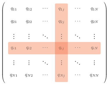
We define and as the sum of the row and the sum of the column respectively of , i.e., and . With a similar abuse of notation, we define as the VOQ set (i.e., those on the row), and as (i.e., those on the column).
Now we introduce a concept that lies at the heart of our derivations: neighborhood. For each VOQ , we define its neighborhood as , the set of VOQs on the row or the column. We denote this neighborhood as , since it has the shape of a cross. With a slight abuse of notation, we use to also denote the set of the corresponding input-output port pairs . Figure 1 illustrates , where the row and column in the shadow are the VOQ sets and respectively. can be viewed as the interference set of VOQs for VOQ [4, 10], as no other VOQ in can be active (i.e., transmit packets) simultaneously with . We define as the total length of all VOQs in (the set) at time slot , that is
| (1) |
Here we need to subtract the term so that it is not double-counted (in both and .
Let be the traffic arrival matrix where is the number of packets arriving at the input port destined for output port during time slot . Here, we assume that, for each , is a sequence of i.i.d. random variables, and this sequence is independent of other sequences (for a different and/or ). Like in [20], we further assume that is upper-bounded by for any at any time slot . Thus, the second moment of their common distribution () is finite. Our analysis, however, holds for more general arrival processes (e.g., Markovian arrivals) that were considered in [4, 10], as we will elaborate shortly. Let be the departure matrix for time slot output by the switching algorithm. Similar to , is a - matrix in which if and only if a packet departs from during time slot . For any , the queue length process evolves as follows:
| (2) |
Let be the (normalized) traffic rate matrix (associated with ) where is normalized (to the percentage of the line rate of an input/output link) mean arrival rate of packets to VOQ . With being an i.i.d. process, we have . We define as the maximum load factor imposed on any input or output port by ,
| (3) |
A switching algorithm is said to achieve 100% throughput or be throughput-optimal if the (packet) queues are stable whenever .
As mentioned before, we will prove in this section that, same as the maximal matching algorithms, QPS-1 is stable under any traffic arrival process , defined above, whose rate matrix satisfies (i.e., can provably attain at least throughput, or half of the maximum). We also derive the average delay bound for QPS-1, which we show is order-optimal (i.e., independent of switch size ). In the sequel, we drop the subscript term from and simply denote it as .
Similar to , we define as the total number of packet arrivals to all VOQs in the neighborhood set :
| (4) |
where and are similarly defined as and respectively. , , and are similarly defined, so is . We now state some simple facts concerning , , and as follows.
Fact 1.
Given any switching algorithm, for any , we have, (at most one packet can depart from input port during time slot ), , and .
Fact 2.
Given any i.i.d. arrival process and its rate matrix is whose maximum load factor is defined in (3), for any , we have .
The following fact is slightly less obvious.
Fact 3.
Given any switching algorithm, for any , we have
| (5) |
4.2 Why QPS-1 Is Just as Good?
The provable throughput and delay bounds of maximal matching algorithms were derived from a “departure inequality” (to be stated and proved next) that all maximal matchings satisfy. This inequality, however, is not in general satisfied by matchings generated by QPS-1. Rather, QPS-1 satisfies a much weaker form of departure inequality (Lemma 1). Fortunately, this much weaker condition is sufficient for proving the same throughput bound and delay bounds, as will be proved in Theorem 1 and Theorem 2 respectively.
Property 1 (Departure Inequality, stated as Lemma 1 in [10, 4]).
If during a time slot , the crossbar schedule is a maximal matching, then each departure process satisfies the following inequality
| (6) |
Proof.
We reproduce the proof of Property 1 with a slightly different approach for this paper to be self-contained. Suppose the contrary is true, i.e., . This can only happen when and . However, implies that no nonempty VOQ (edge) in the neighborhood (see Figure 1) is a part of the matching. Then this matching cannot be maximal (a contradiction) since it can be enlarged by the addition of the nonempty VOQ (edge) . ∎
Clearly, the departure inequality (6) above implies the following much weaker form of it:
| (7) |
In the rest of this section, we prove the following lemma:
Lemma 1.
The matching generated by QPS-1, during any time slot , satisfies the much weaker “departure inequality” (7).
Before we prove Lemma 1, we introduce an important definition and state four facts about QPS-1 that will be used later in the proof. In the following, we will run into several innocuous possible situations that all result from queue-proportional sampling, and we consider all of them to be .
We define as the probability of the event that the proposal from input port to output port is accepted during the accepting phase, conditioned upon the event that input port did propose to output port during the proposing phase. With this definition, we have the first fact
| (8) |
since both sides (note is a 0-1 r.v.) are the probability that proposes to and this proposal is accepted. Summing over on both sides, we obtain the second fact
| (9) |
The third fact is that, for any output port ,
| (10) |
In this equation, the LHS is the conditional probability ( is also a 0-1 r.v.) that at least one proposal is received and accepted by output port , and the second term on the RHS of (10) is the probability that no input port proposes to output port (so receives no proposal). This equation holds since when receives one or more proposals, it will accept one of them (the one with the longest VOQ).
The fourth fact is that, for any ,
| (11) |
This inequality holds because when input port proposes to output port , and no other input port does, has no choice but to accept proposal.
4.3 Proof of Lemma 1
Now we are ready to prove Lemma 1.
By the definition of , we have,
| (12) |
4.4 Throughput Analysis
In this section we prove, through Lyapunov stability analysis, the following theorem (i.e., Theorem 1) which states that any switching algorithm that satisfies the weaker departure inequality (7), including QPS-1 as shown in Lemma 1, can attain at least throughput under i.i.d. arrivals. The same throughput bound was proved in [3], through fluid limit analysis, for maximal matching algorithms using the (stronger) departure inequality (6) which as stated earlier is not in general satisfied by matchings generated by QPS-1.
Theorem 1.
Let be the queueing process of a switching system that is an irreducible Markov chain. Let the departure process of satisfy the weaker “departure inequality” (7). Then whenever its maximum load factor , the queueing process is stable in the following sense: (I) The Markov chain is positive recurrent and hence converges to a stationary distribution ; (II) The first moment of is finite.
Proof.
Here we prove only (I), since Theorem 2 that we will shortly prove implies (II). We define the following Lyapunov function of : , where is defined earlier in (1). This Lyapunov function was first introduced in [4] for the delay analysis of maximal matching algorithms for wireless networking. By the Foster-Lyapunov stability criterion [21, Proposition 2.1.1], to prove that is positive recurrent, it suffices to show that, there exists a constant such that whenever the total queue (VOQ) length (because it is not hard to verify that the complement set of states is finite and the drift is bounded whenever belongs to this set), we have
| (17) |
where is a constant. It is not hard to check (for more detailed derivations, please refer to [4]),
| (18) |
Hence the drift (LHS of (17)) can be written as
| (19) |
Now we claim the following two inequalities, which we will prove shortly.
| (20) | |||
| (21) |
With (20) and (21) substituted into (19), we have
where is a constant. Since , we have . Hence, there exist such that, whenever ,
Now we proceed to prove (20).
| (22) | ||||
| (23) |
In the above derivations, inequality (22) holds due to (7), being independent of for any , and Fact 2 that .
Now we proceed to prove (21), which upper-bounds the conditional expectation . It suffices however to upper-bound the unconditional expectation , which we will do in the following, since we can obtain the same upper bounds on and ( and respectively) whether the expectations are conditional (on ) or not. Note the other two terms and are independent of (the condition) .
As for any , is i.i.d., we have,
| (24) | ||||
| (25) |
Remarks. Now that we have proved that is positive recurrent. Hence, we have, in steady state, for any , . Therefore, we have, in steady state, for any
| (26) |
where is the variance of , because (25) can be simplified as the RHS of (26) in steady state.
Now, we prove the following corollary of Theorem 1 which, in combination with Lemma 1, shows that QPS-1 can attain at least 50% throughput.
Corollary 1.
Under an i.i.d. arrival process, whenever the maximum load factor , QPS-1 is stable in the following sense: The resulting queueing process is a positive recurrent Markov chain and its stationary distribution has finite first moment.
4.5 Delay Analysis
In this section, we derive the bound on the expected total queue length (readily convertible to the corresponding delay bound using Little’s Law) for QPS-1 under i.i.d. traffic arrivals using the following moment bound lemma (i.e., Lemma 2) [21, Proposition 2.1.4]. This bound, shown in (28), is identical to that derived in [4, 10, Section III.B] for maximal matchings under i.i.d. traffic arrivals. Note this equivalence is not limited to i.i.d. traffic arrivals: As will be shown in Section 5.3, the delay analysis results for general Markovian arrivals [20] derived in [4, 10] for maximal matchings (using the stronger “departure inequality” (6)) hold also for QPS-1.
Lemma 2.
Suppose that is a positive recurrent Markov chain with countable state space . Suppose , , and are non-negative functions on such that,
| (27) |
Then , where is a random variable with the stationary distribution of the Markov chain .
Now we derive the following bound on , which is stronger than the part (II) of Theorem 1.
Theorem 2.
Under the same assumptions and definitions as in Theorem 1, we have
| (28) |
Proof.
We replace function in Lemma 2 by , the Lyapunov function used in the proof of Theorem 1 and by the queue length matrix . Let , where , and . It is not hard to check that both and are non-negative functions and inequality (27) holds for defined above. Furthermore, we have proved before, is a positive Markov chain whenever the maximum load factor . Hence, we have, in steady state,
| (29) | ||||
| (30) | ||||
| (31) |
In the above derivation, inequality (29) is because taking expectation on both sides of (20), we have . Thus, we obtain
Inequality (30) is due to Lemma 2, and equality (31) is due to (26).
Therefore, we have, in steady state,
∎
Since, as explained in the proof of Corollary 1, is an irreducible Markov chain under i.i.d. arrivals whose maximum load factor , Theorem 2 applies to QPS-1. Hence we obtain,
Corollary 2.
The bound on as stated in (28) holds under QPS-1 scheduling, whenever the arrival process is i.i.d. and the maximum load factor .
It is not hard to check (by applying Little’s Law) that the average delay (experienced by packets) is bounded by a constant independent of (i.e., order-optimal) for a given maximum load factor , since the variance for any is assumed to be finite in Section 4.1. For the special case of Bernoulli i.i.d. arrival (when ), this bound (the RHS) can be further tightened to . This implies, by Little’s Law, the following “clean” bound: where is the expected delay averaged over all packets transmitting through the switch.
5 Throughput and Delay Analysis under Markovian Arrivals
In this section, we will generalize our results in Section 4 to the more general Markovian arrivals [20].
5.1 Preliminaries
As mentioned earlier the traffic arrival matrix now are Markovian arrivals. More precisely, for any , the number of arrivals for some non-negative integer-valued function , where is an irreducible, positive recurrent and aperiodic discrete-time Markov chain (DTMC) on a finite-state space for some integer and is also an irreducible, positive recurrent and aperiodic DTMC where .
Define the steady-state arrival rate , where is the stationary distribution that converges to. Like in [4, 10], we assume that the underlying DTMC for all is in steady state at time , thus each arrival process is stationary, and therefore, we have, for any and any time slot . Hence, Fact 2 also holds for the arrival process . Like in Section 4.1, we assume that is upper-bounded by for any at any time slot . We further assume that given any integer , there exists some such that for any , where is the matrix with all its entries equal to 0. In other words, the switch could, with a nonzero probability, have no packet arrivals to any of its VOQs during time slots .
As mentioned before, we will prove in this section that, QPS-1 has the same provable throughput and delay guarantees as using maximal matchings under Markovian arrival processes . Before that, we state an fact concerning Markovian arrival processes .
Fact 4.
Given a Markovian arrival process defined above, let be the history of all arrivals (for all VOQs) up to but excluding time slot , then regardless of the past history , we have,
| (32) |
where is some non-negative function of integer such that it converges to exponentially fast as approaches to .
The proof of the above fact can be found in Appendix A.2 of [20].
For any non-negative integer , we define
| (33) |
For any , we define
| (34) |
Note that such a exists because as for any and when , we have for any .
5.2 Throughput Analysis
We now present the throughput result under Markovian arrivals, which generalizes the throughput result under i.i.d. arrivals, i.e., Theorem 1.
Theorem 3.
Let be Markovian arrivals determined by the underlying DTMC as described before in Section 5.1. Suppose the joint process under Markovian arrivals is an irreducible Markov chain. Let the departure process of satisfies the weaker “departure inequality” (7). Then whenever the maximum load factor , the switching system is stable in the following sense: (I) The Markov chain is positive recurrent and hence the queueing process converges in distribution to a stationary distribution ; (II) The first moment of is finite.
Proof.
See B. ∎
5.3 Delay Analysis
Now, we present bounds on the expected total queue length for QPS-1 under Markovian arrivals.
Theorem 4.
Under the same assumptions and definitions as in Theorem 3, we have: (I) The average (total) queue length is upper-bounded as follows.
| (35) |
(II) If arrival processes for different are independent of each other, then the above queue length bound can be further simplified as follows.
| (36) |
where is the steady-sate variance of and is the auto-correlation in in steady state.
Proof.
See D. ∎
Similarly, we have that the bounds on as stated in Theorem 4 hold under QPS-1 scheduling, whenever the arrival processes are Markovian arrivals and the maximum load factor .
6 Evaluation
In this section, we evaluate, through simulations, the performance of QPS-r under various load conditions and traffic patterns. The main purpose of this section to show that QPS-r performs as well as maximal matching algorithms empirically no just in theory. Hence, we do not compare QPS-r with the two recent iterative algorithms in switching 11 1 Note that they are shown to have reasonably good empirical throughput and delay performance over round-robin-friendly workloads such as uniform and hot-spot traffic when running or iterations. However, as described in Section 7, they need to run up to iterations to provably attain at least 50% throughput.: RR/LQF (Round Robin combined with Longest Queue First) [22] and HRF (Highest Rank First) [23]. Instead, we compare its performance with that of iSLIP [7], a refined and optimized representative parallel maximal matching algorithm (adapted for switching). The performance of the MWM (Maximum Weighted Matching) is also included in the comparison as a benchmark. Our simulations show conclusively that QPS-1 (running 1 iteration) performs very well inside the provable stability region (more precisely, with no more than 50% offered load), and that QPS-3 (running iterations) has comparable throughput and delay performances as iSLIP (running iterations), which has a much higher per-port computational complexity of .
6.1 Simulation Setup
In our simulations, we fix the number of input/output ports, to . Later, we investigate how the mean delay performances of these algorithms scale with respect to and the findings are reported in Section 6.3. To measure throughput and delay accurately, we assume each VOQ has an infinite buffer size and hence there is no packet drop at any input port. Each simulation run is guided by the following stopping rule [24, 25]: The number of time slots simulated is the larger between and that is needed for the difference between the estimated and the actual average delays to be within with probability at least .
We assume in our simulations that each traffic arrival matrix is Bernoulli i.i.d. with its traffic rate matrix being equal to the product of the offered load and a traffic pattern matrix (defined next). Similar Bernoulli arrivals were studied in [9, 7, 8]. Later, in Section 6.2.2, we will look at burst traffic arrivals. Note that only synthetic traffic (instead of that derived from packet traces) is used in our simulations because, to the best of our knowledge, there is no meaningful way to combine packet traces into switch-wide traffic workloads. The following four standard types of normalized (with each row or column sum equal to ) traffic patterns are used: (I) Uniform: packets arriving at any input port go to each output port with probability . (II) Quasi-diagonal: packets arriving at input port go to output port with probability and go to any other output port with probability . (III) Log-diagonal: packets arriving at input port go to output port with probability and go to any other output port with probability equal of the probability of output port (note: output port equals output port ). (IV) Diagonal: packets arriving at input port go to output port with probability , or go to output port with probability . These traffic patterns are listed in order of how skewed the volumes of traffic arrivals to different output ports are: from uniform being the least skewed, to diagonal being the most skewed.
6.2 Throughput and Delay Performances

6.2.1 Bernoulli Arrivals
We first compare the throughput and delay performances of QPS-1 (1 iteration), QPS-3 (3 iterations), iSLIP ( = 6 iterations), and MWM (length of VOQ as the weight measure). Note that we have also investigated how the performance of QPS-r scales with respect to , the results are reported in E. Figure 2 shows their mean delays (in number of time slots) under the aforementioned four traffic patterns respectively. Each subfigure shows how the mean delay (on a log scale along the y-axis) varies with the offered load (along the x-axis). We make three observations from Figure 2. First, Figure 2 clearly shows that, when the offered load is no larger than , QPS-1 has low average delays (i.e., more than just being stable) that are close to those of iSLIP and MWM, under all four traffic patterns. Second, the maximum sustainable throughputs (where the delays start to “go through the roof” in the subfigures) of QPS-1 are roughly , and respectively, under the four traffic patterns respectively; they are all comfortably larger than the provable lower bound. Third, the throughput and delay performances of QPS-3 and iSLIP are comparable: The former has slightly better delay performances than the latter under all four traffic patterns except the uniform.
6.2.2 Bursty Arrivals
In real networks, packet arrivals are likely to be bursty. In this section, we evaluate the performances of QPS, iSLIP and MWM under bursty traffic, generated by a two-state ON-OFF arrival process, another special case of Markovian arrivals, described in [4]. The durations of each ON (burst) stage and OFF (no burst) stage are geometrically distributed: the probabilities that the ON and OFF states last for time slots are given by
with the parameters respectively. As such, the average duration of the ON and OFF states are and time slots respectively.
In an OFF state, an incoming packet’s destination (i.e., output port) is generated according to the corresponding load matrix. In an ON state, all incoming packet arrivals to an input port would be destined to the same output port, thus simulating a burst of packet arrivals. By controlling , we can control the desired average burst size while by adjusting , we can control the load of the traffic.
We have evaluated the mean delay performances of QPS-3, iSLIP and MWM, with the average burst size ranging from to packets. We have simulated various offered loads, but here we only present the results, shown in Figure 3, under an offered load of ; other offered loads lead to similar conclusions. Figure 3 clearly shows that QPS-3 outperforms iSLIP (under all traffic patterns except the uniform), by an increasingly wider margin in both absolute and relative terms as the average burst size becomes larger.

6.3 How Mean Delay Scales with N
Figure 4shows how the mean delays of QPS-3, iSLIP (running iterations given any ), and MWM scale with the number of input/output ports , under the four different traffic patterns. We have simulated the following different values of : . In all these plots, the offered load is (Like in Section 6.2.2, we have also simulated other offered loads. They are omitted here, because they lead to similar conclusions), which is quite high compared to the maximum sustainable throughputs of QPS-3 and iSLIP (shown in Figure 2) under these four traffic patterns. Figure 4 shows that the mean delays of QPS-3 are slightly lower (i.e., better) than those of iSLIP under all traffic patterns except the uniform. In addition, the mean delay curves of QPS-3 remain almost flat (i.e., constant) under log-diagonal and diagonal traffic patterns. Although they increase with under uniform and quasi-diagonal traffic patterns, they eventually almost flatten out when gets larger (say when ). These delay curves show that QPS-3, which runs only 3 iterations, deliver slightly better delay performances, under all traffic patterns except the uniform, than iSLIP (a refined and optimized parallel maximal matching algorithm adapted for switching), which runs iterations with each iteration has computational complexity.

7 Related Work
Scheduling in crossbar switches is a well-studied problem with a large amount of literature. So, in this section, we provide only a brief survey of prior work that is directly related to ours, focusing on those we have not described earlier.
Iterative algorithms that compute maximal matchings. As mentioned earlier, maximal matchings have long been recognized as a cost-effective family in switching. Among various types of algorithms that compute maximal matchings, the family of parallel iterative algorithms [23, 22, 26, 27, 28, 29] is widely adopted. Parallel iterative algorithms compute a maximal matching via multiple iterations of message exchanges between the input and output ports. Generally, each iteration contains three stages: request, grant, and accept. In the request stage, each input port sends requests to output ports. In the grant stage, each output port, upon receiving requests from multiple input ports, grants to one. Finally, in the accept stage, each input port, upon receiving grants from multiple output ports, accepts one. Unfortunately, all these parallel iterative algorithms in switching require up to iterations to guarantee that the resulting matching is a maximal matching. In other words, they need up to iterations to achieve the same provable throughput and delay performance guarantees as QPS-1 (running iteration).
Other algorithms that have performance guarantees. Several serial randomized algorithms, starting with TASS [30] and culminating in SERENA [9], have been proposed that have a total computational complexity of only yet can provably attain throughput; SERENA, the best among them, also delivers a good empirical delay performance. However, this complexity is still too high for scheduling high-line-rate high-radix switches, and none of them has been successfully parallelized (i.e., converted to a parallel iterative algorithm) yet, except that SERENA was recently parallelized in [31] that reduces the computational complexity to per port, which is still quite high for high-line-rate high-radix switches.
In [32], a crossbar scheduling algorithm specialized for switching variable-length packets was proposed, that has total computational complexity. Although this algorithm can provably attain throughput, its delay performance is poor. For example, as shown in [8], its average delays, under the aforementioned four standard traffic matrices, are roughly orders of magnitudes higher than those of SERENA [9] even under a moderate offered load of .
8 Conclusion
In this work, we propose QPS-r, a parallel iterative switching algorithm with computational complexity per port. We prove, through Lyapunov stability analysis, that it achieves the same throughput and delay guarantees in theory, and demonstrate through simulations that it has comparable performances in practice as the family of maximal matching algorithms (adapted for switching); maximal matching algorithms are much more expensive computationally (at least iterations and a total of per-port computational complexity). These salient properties make QPS-r an excellent candidate algorithm that is fast enough computationally and can deliver acceptable throughput and delay performances for high-link-rate high-radix switches.
References
- [1] C. Cakir, R. Ho, J. Lexau, K. Mai, Modeling and Design of High-Radix On-Chip Crossbar Switches, in: Proc. of the ACM/IEEE NoCS, Vancouver, BC, Canada, 2015, pp. 20:1–20:8.
- [2] C. Cakir, R. Ho, J. Lexau, K. Mai, Scalable High-Radix Modular Crossbar Switches, in: Proceedings of the HOTI, Santa Clara, CA, USA, 2016, pp. 37–44.
- [3] J. Dai, B. Prabhakar, The Throughput of Data Switches with and without Speedup, in: Proceedings of the IEEE INFOCOM, Tel Aviv, Israel, 2000, pp. 556–564.
- [4] M. J. Neely, Delay Analysis for Maximal Scheduling in Wireless Networks with Bursty Traffic, in: Proceedings of the IEEE INFOCOM, 2008.
- [5] A. Israel, A. Itai, A Fast and Simple Randomized Parallel Algorithm for Maximal Matching, Inf. Process. Lett. 22 (2) (1986) 77–80.
- [6] T. E. Anderson, S. S. Owicki, J. B. Saxe, C. P. Thacker, High-speed Switch Scheduling for Local-area Networks, ACM Trans. Comput. Syst. 11 (4) (1993) 319–352.
- [7] N. McKeown, The iSLIP Scheduling Algorithm for Input-queued Switches, IEEE/ACM Trans. Netw. 7 (2) (1999) 188–201.
- [8] L. Gong, P. Tune, L. Liu, S. Yang, J. J. Xu, Queue-Proportional Sampling: A Better Approach to Crossbar Scheduling for Input-Queued Switches, Proceedings of the ACM SIGMETRICS 1 (1) (2017) 3:1–3:33.
- [9] P. Giaccone, B. Prabhakar, D. Shah, Randomized Scheduling Algorithms for High-Aggregate Bandwidth Switches, IEEE J. Sel. Areas Commun. 21 (4) (2003) 546–559.
- [10] M. J. Neely, Delay Analysis for Maximal Scheduling With Flow Control in Wireless Networks With Bursty Traffic, IEEE/ACM Trans. Netw. 17 (4) (2009) 1146–1159.
- [11] D. J. Aweya, Switch/Router Architectures: Shared-Bus and Shared-Memory Based Systems, 1st Edition, Wiley-IEEE Press, 2018.
- [12] Y. Tamir, G. L. Frazier, High-performance Multi-queue Buffers for VLSI Communications Switches, SIGARCH Comput. Archit. News 16 (2) (1988) 343–354.
- [13] M. Karol, M. Hluchyj, S. Morgan, Input Versus Output Queueing on a Space-Division Packet Switch, IEEE Trans. Commun. 35 (12) (1987) 1347–1356.
- [14] L. Tassiulas, A. Ephremides, Stability properties of constrained queueing systems and scheduling policies for maximum throughput in multihop radio networks, IEEE Transactions on Automatic Control 37 (12) (1992) 1936–1948.
- [15] N. McKeown, A. Mekkittikul, V. Anantharam, J. Walrand, Achieving 100% Throughput in an Input-Queued Switch, IEEE Trans. Commun. 47 (8) (1999) 1260–1267. doi:10.1109/26.780463.
- [16] L. Tassiulas, A. Ephremides, Stability Properties of Constrained Queueing Systems and Scheduling Policies for Maximum Throughput in Multihop Radio Networks, IEEE Trans. Autom. Control 37 (12) (1992) 1936–1948.
- [17] D. Shah, M. Kopikare, Delay bounds for approximate maximum weight matching algorithms for input queued switches, in: Proceedings of the IEEE INFOCOM, Vol. 2, 2002, pp. 1024–1031 vol.2.
- [18]
R. Duan, H.-H. Su, A
Scaling Algorithm for Maximum Weight Matching in Bipartite Graphs, in:
Proceedings of the ACM-SIAM SODA, 2012, pp. 1413–1424.
URL http://dl.acm.org/citation.cfm?id=2095116.2095227 - [19] I. Keslassy, R. Zhang-Shen, N. McKeown, Maximum size matching is unstable for any packet switch, IEEE Communications Letters 7 (10) (2003) 496–498. doi:10.1109/LCOMM.2003.817330.
- [20] S. Mou, S. T. Maguluri, Heavy traffic queue length behaviour in a switch under markovian arrivals (2020). arXiv:2006.06150.
- [21] B. Hajek, Notes for ece 467 communication network analysis, http://www.ifp.illinois.edu/˜hajek/Papers/networkanalysisDec06.pdf (2006).
- [22] B. Hu, K. L. Yeung, Q. Zhou, C. He, On Iterative Scheduling for Input-Queued Switches With a Speedup of , IEEE/ACM Trans. Netw. 24 (6) (2016) 3565–3577.
- [23] B. Hu, F. Fan, K. L. Yeung, S. Jamin, Highest Rank First: A New Class of Single-Iteration Scheduling Algorithms for Input-Queued Switches, IEEE Access 6 (2018) 11046–11062.
- [24] J. M. Flegal, G. L. Jones, et al., Batch means and spectral variance estimators in Markov chain Monte Carlo, Ann. Stat. 38 (2) (2010) 1034–1070.
- [25] P. W. Glynn, W. Whitt, et al., The Asymptotic Validity of Sequential Stopping Rules for Stochastic Simulations, Ann. Appl. Probab. 2 (1) (1992) 180–198.
- [26] Yihan Li, S. Panwar, H. J. Chao, On The Performance of A Dual Round-Robin Switch, in: Proceedings of the IEEE INFOCOM, Anchorage, AK, USA, 2001, pp. 1688–1697 vol. 3.
- [27] N. W. McKeown, Scheduling Algorithms for Input-queued Cell Switches, Ph.D. thesis, Berkeley, CA, USA, uMI Order No. GAX96-02658 (1995).
- [28] A. Scicchitano, A. Bianco, P. Giaccone, E. Leonardi, E. Schiattarella, Distributed Scheduling in Input Queued Switches, in: Proceedings of the IEEE ICC, 2007, pp. 6330–6335.
- [29] D. Lin, Y. Jiang, M. Hamdi, Selective-Request Round-Robin Scheduling for VOQ Packet Switch Architecture, in: Proceedings of the IEEE ICC, 2011, pp. 1–5.
- [30] L. Tassiulas, Linear Complexity Algorithms for Maximum Throughput in Radio Networks and Input Queued Switches, in: Proceedings of the IEEE INFOCOM, San Francisco, CA, USA, 1998, pp. 533–539.
- [31] L. Gong, L. Liu, S. Yang, J. J. Xu, Y. Xie, X. Wang, Serenade: A parallel iterative algorithm for crossbar scheduling in input-queued switches, in: 2020 IEEE 21st International Conference on High Performance Switching and Routing (HPSR), 2020, pp. 1–6.
- [32] S. Ye, T. Shen, S. Panwar, An Scheduling Algorithm for Variable-Size Packet Switching Systems, in: Proceedings of the 48th Annual Allerton Conference, 2010, pp. 1683–1690.
- [33] G. Fayolle, V. A. Malyshev, M. V. Menshikov, Topics in the constructive theory of countable Markov chains, Cambridge university press, 1995.
Appendix A Irreducibility of
We have shown that the queueing process is a Markov chain in the proof of Corollary 1. Now we prove that this Markov is irreducible using the same approach as used in [8]. Here we provide only a proof sketch. We show that the queueing process , starting from any state (i.e., VOQ lengths) it is currently in, will with a positive probability return to the state, in which all VOQs have a length of , in a finite number of steps (i.e., time slots). To show this property, we claim that, for any integer , the switch could, with a nonzero probability, have no packet arrivals to any of its VOQs during time slots . This claim is true because, the arrival process is i.i.d., and for any and , we have (since the maximum load factor ). Hence, when there are no packet arrivals during time slots , which happens with a nonzero probability, QPS-1 can clear all the queues during this period, with a sufficiently large , and return the queueing process to the state. Therefore, the Markov chain is irreducible.
Appendix B Proof of Theorem 3
In this section, we prove Theorem 3. The proof follows the same outline as the proof of Theorem 1 with some necessary modifications to allow for Markovian arrivals. Note that we prove only (I) here, since Theorem 4 that we will shortly prove implies (II).
For notational convenience, we define . Unlike in the proof of Theorem 1 where we use the 1-step Foster-Lyapunov stability criterion [21, Proposition 2.1.1], here we use the -step (multiple-step) Foster-Lyapunov stability criterion [33, Theorem 2.2.4]. We consider again the following Lyapunov function: , and show that its -step drift, which is defined as , is negative except in a finite set.
To compute the -step drift, we first compute,
| (37) |
Thus, the term in the first term on the RHS of (37) can be written as
| (40) |
Focusing on the second term above and using (1), we have
| (42) |
Hence, the drift can be written as
| (43) |
Since and , for any and , we have
| (44) |
where .
Now we claim there exists some (where is defined in (34)) such that the following inequality holds, which we will prove shortly.
| (45) |
Define . Such an should exist because and as . Define , clearly . With (44) and (45) substituted into (43), we have
| (46) |
where .
Inequality (46) is due to and (since each is a DTMC on a finite-state space of ). Because , there exist such that, whenever ,
Now we proceed to prove (45). By simple calculations, we have
| (47) |
Focusing on the first term in the parentheses above, for the conditional expectation , we have
| (48) |
Since for any and , we have the first expectation above, , is bounded by
| (49) |
Therefore, the second expectation on the RHS of (48), , can be bounded by
| (50) |
Now, we proceed to bound the second term in the parentheses on the RHS of (47), .
Using (2), we have for any integer . Because and for any and , for any integer . Thus, for any integer , we have
| (51) | ||||
| (52) | ||||
| (53) | ||||
| (54) |
Inequality (51) is due to for any and . Inequality (52) is due to (7) and inequality (53) is due to and for any and .
Using (54), we have
| (55) |
Appendix C Theorem 3Applies to QPS-1
In this section, we prove that Theorem 3 applies to QPS-1. More precisely, under Markovian arrivals whenever the maximum load factor , QPS-1 is stable in the following sense: The resulting joint process is a positive recurrent Markov chain and the stationary distribution of the queueing process has finite first moment.
The joint process is a Markov chain, by the following two facts. First, is a Markov chain so only depends on . Second, by (2), depends on only and , where is a function of only and is a function of only .
The reasoning for the irreducibility of this Markov chain is almost identical to those in A, so we omit it here for brevity.
Appendix D Proof of Theorem 4
Part (I). Now we prove (I) in Theorem 4. Like in B, we let . Like in the proof of Theorem 2, we replace function in Lemma 2 by , the Lyapunov function used in the proof of Theorem 3 and by . We define and functions in the same way as in the proof of Theorem 2. First, we show that the , , , and defined above satisfy (27).
Now we claim the following two inequalities that hold in steady state of the positive recurrent Markov chain , which we will prove shortly.
| (57) |
| (58) |
Then, using similar reasoning as in the proof of Theorem 2, we have
Therefore, we have, in steady state,
Now we proceed to prove (57).
| (59) |
Focusing on the first expectation term, , above, we have
| (60) | ||||
| (61) | ||||
| (62) | ||||
| (63) | ||||
| (64) |
(60)is due to (2). Inequality (61) is due to for any and . Inequality (62) is due to Fact 4. Inequality (63) is due to (33).
Using the weak departure inequality (7), we have the second expectation term on the RHS of (59),
Therefore, we have, in steady state
| (65) | ||||
| (66) |
(65) is due to the fact for any in steady state.
Now we prove (58). By simple calculations, we have
| (67) | ||||
| (68) |
In arriving at (67), we have used Fact 3, i.e., for any , . Inequality (68) is due to for any at any time slot .
We note that is positive recurrent. Therefore, we have, in steady state, for any , . Hence, we have, in steady state,
Part (II). Now we proceed to prove (II). Since any now is independent of each other, we have, for any
| (69) |
where is the steady-state variance of .
Similarly, we have, for any , any and any integer
| (70) |
where is the auto-correlation in in steady state.
Appendix E How Mean Delay of QPS-r Scales with r

Figure 5presents the mean delay performance of QPS-r, with , as a function of the offered loads, under Bernoulli i.i.d. arrivals with the traffic patterns. It shows that both the maximum sustainable throughput and the mean delay performance improve as increases. However, as , the improvement becomes marginal.