Accuracy Improvement of Neural Network Training using Particle Swarm Optimization and its Stability Analysis for Classification

FFNN is, one of the kind of Multi-Layer Perceptron (MLP)  Savran 2007, most popularly and most widely used model in many practical applications because of their high capability to forecasting and classification. MLP with three layers( First, input layer ($IL$); Second, hidden layer ($HL$); Last, output layer ($OL$)) is more popular Irie and Miyake 1988. The inputs (n attributes) or features of an example to be classified are entered into the $IL$. The $OL$ typically consists of as many outputs as classes in classification problem. Information flows from $IL$ to $HL$ and then to $OL$ via a set of arcs N. 2012. The basic computational element or building block of neural network is called neuron. It is to be noted that within the layer nodes are not directly connected. Figure. (1) is an example.

The input to the hidden node j is obtained as

$${IH_{j}}=\sum\limits_{j=1}^{n}{{W_{ij}}^{(1)}{O_{i}}+{b_{j}}}$$

(1)

and output of hidden layer is

$${OH_{j}}=af(I{H_{j}})$$

(2)

where $n$ is the number of neurons present in the $HL$. ${W_{ij}}^{(k)}$ is the synaptic weight for the connection linking node $i$ in the ${K^{th}}$ layer of nodes to $j$. $af$ is the activation function (AF). Here the AF is considered as sigmoid function:

$$af(I{H_{j}})=\frac{1}{{1+{e^{-I{H_{j}}}}}}$$

(3)

The input of an output node IO

$${IO_{j}}=\sum\limits_{i=1}^{z}{{W_{ij}}^{(2)}*O{H_{i}}}$$

(4)

and output of $OL$ is

$${OO_{j}}=af(I{O_{j}})$$

(5)

where $z$ is number of hidden nodes. The outputs are non linearly related to inputs. The FFNN which is being considered for the problem of classification as pictured in Fig (1). The range for output lie in [0, 1]. For each of the training examples in the training set($T_{set}$), its inputs are feeded to the FFNN and obtained (or predicted) outputs are calculated. The difference between each obtained (or predicted) and the corresponding targeted (or actual) output is calculated. The total error ($Err$) of the network is

$$Err=\frac{1}{2}\sum\limits_{i=1}^{|T_{set}|}{{{(T{O_{i}}-O{O_{i}})}^{2}}}$$

(6)

where $TO_{i}$ and $OO_{i}$ are the targeted (or actual) and obtained (or predicted) outputs, respectively, for $i^{th}$ training example. Training of FFNN is nothing but minimizing the mean square error($MSE$). A separate error value (${Err}$) can be expressed as the parameters in the network as follows:

	$\displaystyle Err=\frac{1}{2}\sum\limits_{t=1}^{|T_{set}|}{{{(T{O_{i}}-af(\sum\limits_{i=1}^{z}{{W_{ij}}^{(2)}O{H_{i}}}))}^{2}}}$
	$\displaystyle=\frac{1}{2}\sum\limits_{t=1}^{|T_{set}|}{{{(T{O_{i}}-af(\sum\limits_{i=1}^{z}{{W_{ij}}^{(2)}af(\sum\limits_{j=1}^{n}{{W_{ij}}^{(1)}{O_{i}}+{b_{j}}})}))}^{2}}}$

The learning algorithm typically repeated through $T_{set}$ many times- each repetition (or cycle) is called $epoch$ in the ANN literature.

PSO is a stochastic population based meta-heuristic algorithm first introduced by Kennedy and Eberhart in 1995  Kennedy and Eberhart 1995. Suppose that the size of the swarm is $noP$ (population size) and the search space is $D$ - dimensional.

The position of the $i^{th}$ particle is presented as $x_{id}={\rm{(}}x_{i1},x_{i2},.{\rm{}}.{\rm{}}.,x_{iD})$ where $x_{id}\in[l{b_{d}},u{b_{d}}]$, $d\in[1,D]$ and $lb_{d}$ and $ub_{d}$ are the lower and upper bounds of the $d^{th}$ dimension of the search space. The $i^{th}$ particle velocity is presented as $v_{i}={\rm{}}(v_{i1},v_{i2},.{\rm{}}.{\rm{}}.,v_{iD})$. At each time step, the position and velocity of the particles are updated according to the following equations:

	$\displaystyle v_{ij}(t+1)=\omega*v_{ij}(t)+{c_{1}}*{r_{1}}*\left({{p^{lB}}_{ij}(t)-x_{ij}(t)}\right)$
	$\displaystyle+{c_{2}}*{r_{2}}*\left({{p^{gB}}_{j}(t)-x_{ij}(t)}\right)$		(7)

$$x_{ij}(t+1)=x_{ij}(t)+v_{ij}(t+1)$$

(8)

where ${r_{1}},{r_{2}}$ are two distinct random numbers, generated uniformly from the range [0, 1], ${c_{1}},{c_{2}}$ are acceleration coefficients and $t$ is the current iteration. The best previous position found so far by the particle is denoted as ${p^{lB}_{i}}{\rm{}}$, and the best previous position discovered by the whole swarm is denoted as ${p^{gB}}{\rm{}}$. The velocity of particle should be under the constrained conditions ${\left[{{v_{min}},{\rm{}}{v_{max}}}\right]^{D}}$. In Eq. (9), ${\omega}*v_{ij}(t)$ , provides exploration ability for PSO. The second part ${c_{1}}*{r_{1}}*\left({{p^{lB}}_{ij}(t)-x_{ij}(t)}\right)$ and third part ${c_{2}}*{r_{2}}*\left({{p^{gB}}_{j}(t)-x_{ij}(t)}\right)$ represent private thinking and collaboration of particles respectively.

It has been proved by experiments that truly random initialization of particles position in search space can enhance the exploration of various regions in search space and can also enhance the performance of the PSO. Hence classification performance of FFNN will be increased. However computers can’t provide truly random numbers via pseudo random generators, which means optimal discrepancy is not achievable by them.

Figure. (2) shows the difference between pseudo random and Sobol random initialization.

So, many researchers have studied alternative ways to generate low-discrepancy sequences. Uy et al. 2007 have investigated some of well-known randomized low-discrepancy sequences (Sobol, Halton and Faure) for the PSO position initialization. So, according to the research, PSO initialization with Sobol sequences is recommended Jordehi and Jasni 2013.

Shi and Eberhart 2001 claimed that a large $IW$ facilitates a global search while a small $IW$ facilitates a local search.

In this experiment, 8 different datasets are used. All are collected from UCI repository  Dua and Karra Taniskidou 2017. Data normalization is done in the range between [-1, 1] and there is no missing value present in dataset. The details of data sets are mentioned TABLE (1):

“Hold Out” cross validation method has been used for the data division where 80$\%$ instances of data are used for training the FFNN and rest 20$\%$ instances of data are used to test the trained FFNN.

In this experiment, the population size (${noP}$) is 50, $I_{max}$ is 500, and initialization of $p_{i}$ and $v_{i}$ are initialized by Sobol random initializer. In PPSO $c_{1}$ and $c_{2}$ are 1.6 and 1.7 respectively and $IW$ increases linearly from 0.4 to 0.9. In BPSO $c_{1}$and $c_{2}$ both are set to 1.5 and $IW$ is varying inertia with value is decreasing from ${\omega}_{max}$ ${=0.9}$ to ${\omega}_{max}$ ${=0.3}$. In SGPSO, $c_{1}$,$c_{2}$ and $IW$ all are same as BPSO and $c_{3}$ is 0.5. For SGPSO geometric center is 100 Garro and Vázquez 2015. In PSOGSA $c_{1}$ and $c_{2}$ both are set to 1 and $IW$ linearly decreases from ${\omega}_{max}$ ${=0.9}$ to ${\omega}_{max}$ ${=0.5}$. In GSA, gravitational constant value ( $G_{0}$) is set to 1 and initial values for $mass$ and $acceleration$ are set to 0.

For the classification accuracy (testing accuracy) measurement Confusion Matrix is used. Confusion Matrix is very useful tool in order to analyze the accuracy Han et al. 2011, that how efficiently the classifier can able to recognize different classes. The classifier is also evaluated using standard metrics: Precision (Pre), Recall (Rec), and F-Measure (FM) [11] Aggarwal 2014 :

$$FM=2*(\frac{{Pre*Rec}}{{Pre+Rec}})$$

(11)

where $Pre=\frac{{Tp}}{{Tp+Fp}}$ and $Rec=\frac{{Tp}}{{Tp+Fn}}$. True positives ($Tp$): number of incorrect samples correctly identified as incorrect; true negatives ($Tn$): number of normal samples correctly identified as normal; false positives ($Fp$): number of normal samples misclassified as incorrect; false negatives ($Fn$): number of incorrect samples misclassified as normal. Here FM is the weighted average of Precision and Recall. Therefore, this score takes both false positives and false negatives into account.

From eq.7 and 8 each dimension is updated independently from other dimensions. The relation between the dimensions and problem space is the global best position ${p^{gB}}$ found so far. So, without loss of generality, the algorithm can be reduced to one dimensional case for analysing purpose:

$$v(t+1)=\omega*v(t)+\psi_{1}*\left({{p^{lB}}-x(t)}\right)+\psi_{2}*\left({{p^{gB}}-x(t)}\right)$$

(12)

$$x(t+1)=x(t)+v(t+1)$$

(13)

where $\psi_{1}$=$c_{1}*r_{1}$ and $\psi_{2}$=$c_{2}*r_{2}$.
Let

	$\displaystyle\psi=\psi_{1}+\psi_{2}$
	$\displaystyle p=\frac{\psi_{1}p^{lB}+\psi_{2}p^{gB}}{\psi}$

Then Eq.12 and 13 can be simplified as

$$v(t+1)=\omega v(t)-\psi x(t)+\psi p$$

(14)

$$x(t+1)=\omega v(t)+(1-\psi)x(t)+\psi p$$

(15)

where $\psi$ is the new attraction coefficient, which is the combination of cognitive behaviour (local search) and social behaviour (global attraction) $\psi 1$ and $\psi 2$. The attraction point($p$) is weighted average of global best($p^{gB}$) and local best ($p^{lB}$) in the swarm.
Dynamic Analysis: For dynamic analysis  Clerc and Kennedy 2002, let

$\displaystyle y_{t}=x_{t}-p$

(16)

Now Eq. 14 and 15 can be simplified as:

$$v(t+1)=\omega v(t)-\psi y(t)$$

(17)

$$y(t+1)=\omega v(t)+(1-\psi)y(t)$$

(18)

Let

$${X_{t}}=\left(\begin{array}[]{l}{v_{t}}\\ {x_{t}}\end{array}\right)$$

(19)

then Eq.(17) and 18 can be written in matrix-vector form:

$$X_{t+1}=GX_{t}$$

(20)

so,

$$\left(\begin{array}[]{l}{v_{t+1}}\\ {x_{t+1}}\end{array}\right)=\left({\begin{array}[]{*{20}{c}}\omega&{-\psi}\\ \omega&{1-\psi}\end{array}}\right)\left(\begin{array}[]{l}{v_{t}}\\ {x_{t}}\end{array}\right)$$

(21)

where the coefficient matrix is $G$

$\displaystyle G=\left({\begin{array}[]{*{20}{c}}\omega&{-\psi}\\ \omega&{1-\psi}\end{array}}\right)$

The eigenvalues of the $G$ can be obtained by solving the following equation for $\lambda$ :

$$\det\begin{pmatrix}\omega-\lambda&-\psi\\ \omega&(1-\psi)-\lambda\end{pmatrix}=0$$

(24)

$$\Rightarrow(\omega-\lambda)(1-\psi-\lambda)+\omega\psi=0$$

$$\Rightarrow{\lambda^{2}}-\lambda(1-\psi)-\omega\lambda+(\omega(1-\psi)+\omega\psi)=0$$

$$\Rightarrow{\lambda^{2}}-\lambda((1-\psi)+\omega)+\det(G)=0$$

$\displaystyle\Rightarrow{\lambda^{2}}-Tr(G)\lambda+\det(G)=0$

(25)

where $\det(G)$ is the determinant of coefficient matrix $G$.

$$\det(G)=det\left({\begin{array}[]{*{20}{c}}\omega&{-\psi}\\ \omega&{1-\psi}\end{array}}\right)=\omega$$

$Tr(G)$ is trace of matrix $G$ which is equal to the summation of principal diagonal elements. Here

$$Tr(G)=\omega+1-\psi$$

Eq. 25 is the characteristic equation. Where $\lambda$ is the eigen value which is a solution to the eq 25. Now

$$\lambda=\frac{{Tr(G)\pm\sqrt{Tr{{(G)}^{2}}-4del(G)}}}{2}$$

Now for checking the condition in which the system is stabile. The real part of eigen value ( $Re(\lambda)$ ) can be given as follows:

$${\mathop{\rm Re}\nolimits}(\lambda)=\left\{\begin{array}[]{l}\frac{{Tr(G)}}{2}\hskip 14.22636ptif\hskip 14.22636ptTr{(G)^{2}}<4\det(G)\\ \frac{{Tr(G)+\sqrt{Tr{{(G)}^{2}}-4\det(G)}}}{2}\hskip 5.69046ptif\hskip 5.69046ptTr{(G)^{2}}\geq 4\det(G)\end{array}\right.$$

If $Tr{(G)^{2}}<4\det(G)$, the stability condition is as follows:

$\displaystyle Tr(G)<0$

(26)

If $Tr{(G)^{2}}\geq 4\det(G)$, the stability condition can be derived as follows:

$${Tr(G)+\sqrt{Tr{{(G)}^{2}}-4\det(G)}}<0$$

$$\Rightarrow{\sqrt{Tr{{(G)}^{2}}-4\det(G)}}<-Tr(G)$$

squaring bothsides the following can be achieved

$$\Rightarrow{\sqrt{Tr{{(G)}^{2}}-4\det(G)}}<Tr(G)^{2}$$

so,

$\displaystyle det(G)>0$

(27)

By substituting $Tr(G)=\omega+1-\psi$ to eq.(26) the follwing can be concluded

$$\omega+1-\psi<0$$

$\displaystyle\Rightarrow\omega<\psi-1$

(28)

By substituting $det(G)=\omega$ to eq.(27) the follwing can be concluded that

$\displaystyle\omega>0$

(29)

By combining all the results above, the conclusion can be drawn that the proposed PPSO is stable and its stability depends on $\omega$. The range of $\omega$ for which the PPSO is stable is $0<\omega<(\psi-1)$. Hence the proposed PPSO is stable.

The $F$-measure and accuracy from best run are reported in TABLE ( 3 ) and TABLE (2) respectively for BPSO, SGPSO, GSA, PSOGSA and PPSO classifiers. The results in boldface in tables are showing better in comparative analysis of four above mentioned classifiers.

Table (2), reports the accuracy comparison of the proposed PPSO classifier with 4 other classifiers (i,e BPSO, SGPSO, GSA, PSOGSA). It can be reported that on all datasets PPSO has outperformed BPSO, SGPSO, GSA.And PPSO outperformed PSOGSA in 7 datasets out of 8 datasets and achieved better classification accuracy than PSOGSA. But there is a tie between PSOGSA and PPSO, both have achieved 100% classification accuracy on Iris dataset.

From TABLE (3), the PPSO classifier showed better performance in 7 out of 8 datasets. But PSOGSA classifier, among 8 datasets 1 dataset (i,e Balance Scale) has shown better FM value than PPSO.

Figure (3) reports the convergence curves while training the FFNN using BPSO, SGPSO, GSA, PSOGSA and PPSO. One dataset ( i,e banknote dataset) is reported for the convergence curve plot. It can be seen that the convergence of PPSO is better than other classifiers.

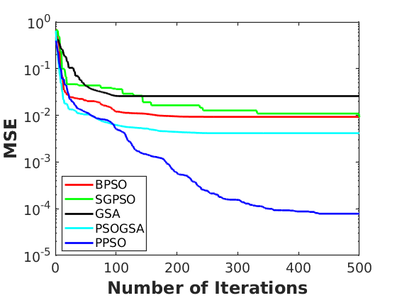
Figure (4) reports the confusion matrix (a measurement between target class(actual class) vs output class (FFNN produced class)) comparison among 5 classifiers (BPSO, SGPSO, GSA, PSOGSA and PPSO) for classification of cancer dataset. In confusion matrix plot green colored cells are the classes which are correctly classified and red colored cells are the classes which are misclassified by the classifier for the cancer test dataset. It also shows the accuracy of all the classifiers. Subfigure 4, 4, 4, 4, 4  are the confusion matrix plot for BPSO, SGPSO, GSA, PSOGSA, PPSO classifier’s respectively. And the difference among classifiers are clearly visible. Where BPSO, SGPSO, GSA, PSOGSA ans PPSO all can able to classify 102, 103, 105, 107, 109 samples out of 114 samples in cancer test dataset. The accuracy achieved by BPSO, SGPSO, GSA, PSOGSA, PPSO are 89.5, 90.4, 92.1, 93.9, 95.6 respectively. So, it can easily be seen that PPSO classifier is better than other 4 classifiers.

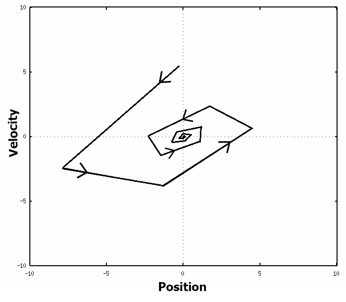
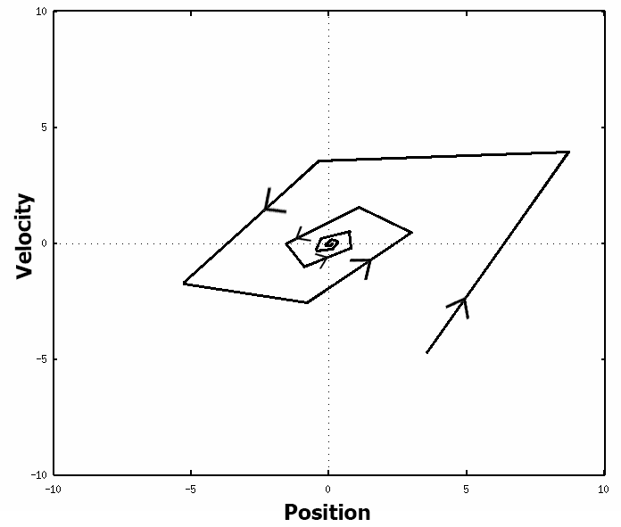
Figure 5 presents the phase trajectory of the proposed algorithm with different initial points. This experiment has been done using XPPAUT 8.0 Ermentrout 2016. From this phase trajectory, it can be concluded that whatever be the initial position of particle is, proposed inertial weight strategy ($\omega$) will converge to a stable fixed point. It is mentioned that range of $\omega$ must be within the range $0<\omega<\psi-1$. Hence, it is obvious that, proposed system is stable by analytically as well as experimentally.

References

- Aggarwal [2014] Charu C. Aggarwal. Data Classification: Algorithms and Applications. Chapman & Hall/CRC, 1st edition, 2014.
- Agrawal and Bawane [2015] Rajesh K. Agrawal and Narendra G. Bawane. Multiobjective pso based adaption of neural network topology for pixel classification in satellite imagery. Applied Soft Computing, 28:217 – 225, 2015.
- Behrang et al. [2011] M.A. Behrang, E. Assareh, M. Ghalambaz, M.R. Assari, and A.R. Noghrehabadi. Forecasting future oil demand in iran using gsa (gravitational search algorithm). Energy, 36(9):5649 – 5654, 2011.
- Clerc and Kennedy [2002] M. Clerc and J. Kennedy. The particle swarm - explosion, stability, and convergence in a multidimensional complex space. IEEE Transactions on Evolutionary Computation, 6(1):58–73, Feb 2002.
- Dua and Karra Taniskidou [2017] Dheeru Dua and Efi Karra Taniskidou. UCI machine learning repository, 2017.
- Ermentrout [2016] Bard Ermentrout. Xppaut 8.0 january 2016, 2016.
- Garro and Vázquez [2015] Beatriz A. Garro and Roberto A. Vázquez. Designing artificial neural networks using particle swarm optimization algorithms. Computational Intelligence and Neuroscience 2015, 2015:369298– 20, 2015.
- Han et al. [2011] Jiawei Han, Micheline Kamber, and Jian Pei. Data Mining: Concepts and Techniques. Morgan Kaufmann Publishers Inc., San Francisco, CA, USA, 3rd edition, 2011.
- Hornik et al. [1989] Kurt Hornik, Maxwell Stinchcombe, and Halbert White. Multilayer feedforward networks are universal approximators. Neural Networks, 2(5):359 – 366, 1989.
- Hu et al. [2017] Hongping Hu, Xiaxia Cui, and Yanping Bai. Two kinds of classifications based on improved gravitational search algorithm and particle swarm optimization algorithm. Advances in Mathematical Physics, 2017:1–7, 09 2017.
- Irie and Miyake [1988] B. Irie and Shogo Miyake. Capabilities of three-layered perceptrons. IEEE 1988 International Conference on Neural Networks, pages 641–648 vol.1, 1988.
- Jordehi and Jasni [2013] A. Rezaee Jordehi and J. Jasni. Parameter selection in particle swarm optimisation: a survey. Journal of Experimental & Theoretical Artificial Intelligence, 25(4):527–542, 2013.
- Kar and Kelkar [2013] S. A. Kar and V. V. Kelkar. Classification of multispectral satellite images. In 2013 International Conference on Advances in Technology and Engineering (ICATE), pages 1–6, Jan 2013.
- Kattan et al. [2010] A. Kattan, R. Abdullah, and R. A. Salam. Harmony search based supervised training of artificial neural networks. In 2010 International Conference on Intelligent Systems, Modelling and Simulation, pages 105–110, Jan 2010.
- Kennedy and Eberhart [1995] J. Kennedy and R. Eberhart. Particle swarm optimization. In Proceedings of ICNN’95 - International Conference on Neural Networks, volume 4, pages 1942–1948 vol.4, Nov 1995.
- Lu et al. [2015] Yang Lu, Gang Lu, Xianye Bu, Yajing Yu, and Xianye Bu. Classification of hand manipulation using bp neural network and support vector machine based on surface electromyography signal. IFAC-PapersOnLine, 48(28):869 – 873, 2015. 17th IFAC Symposium on System Identification SYSID 2015.
- Malakooti and Zhou [1998] Behnam Malakooti and YingQing Zhou. Approximating polynomial functions by feedforward artificial neural networks: Capacity analysis and design. Applied Mathematics and Computation, 90(1):27 – 51, 1998.
- Mirjalili et al. [2012] SeyedAli Mirjalili, Siti Zaiton Mohd Hashim, and Hossein Moradian Sardroudi. Training feedforward neural networks using hybrid particle swarm optimization and gravitational search algorithm. Applied Mathematics and Computation, 218(22):11125 – 11137, 2012.
- Montana and Davis [1989] David J. Montana and Lawrence Davis. Training feedforward neural networks using genetic algorithms. In Proceedings of the 11th International Joint Conference on Artificial Intelligence - Volume 1, IJCAI’89, pages 762–767, San Francisco, CA, USA, 1989. Morgan Kaufmann Publishers Inc.
- N. [2012] Oza N. Classification, pages 505–522. Chapman & Hall/CRC, 1st edition, March 2012. Provided by the SAO/NASA Astrophysics Data System.
- Rakitianskaia et al. [2016] A. Rakitianskaia, E. Bekker, K. M. Malan, and A. Engelbrecht. Analysis of error landscapes in multi-layered neural networks for classification. In 2016 IEEE Congress on Evolutionary Computation (CEC), pages 5270–5277, July 2016.
- Rashedi et al. [2011] Esmat Rashedi, Hossien Nezamabadi-pour, and Saeid Saryazdi. Filter modeling using gravitational search algorithm. Engineering Applications of Artificial Intelligence, 24(1):117 – 122, 2011.
- Savran [2007] A. Savran. Multifeedback-layer neural network. IEEE Transactions on Neural Networks, 18(2):373–384, March 2007.
- Settles and Rylander [2002] Matt Settles and Bart Rylander. Neural network learning using particle swarm optimization. In Advances in Information Science and SoftComputing, pages 224–226, 2002.
- Shi and Eberhart [2001] Yuhui Shi and R. C. Eberhart. Fuzzy adaptive particle swarm optimization. In Proceedings of the 2001 Congress on Evolutionary Computation (IEEE Cat. No.01TH8546), volume 1, pages 101–106 vol. 1, May 2001.
- Uy et al. [2007] Nguyen Quang Uy, Nguyen Xuan Hoai, R. McKay, and P. M. Tuan. Initialising pso with randomised low-discrepancy sequences: the comparative results. In 2007 IEEE Congress on Evolutionary Computation, pages 1985–1992, Sep. 2007.
- Vazquez and Garro [2016] Roberto A. Vazquez and Beatriz A. Garro. Crop classification using artificial bee colony (abc) algorithm. In Ying Tan, Yuhui Shi, and Li Li, editors, Advances in Swarm Intelligence, pages 171–178, Cham, 2016. Springer International Publishing.
- Zhang [2000] G. P. Zhang. Neural networks for classification: a survey. IEEE Transactions on Systems, Man, and Cybernetics, Part C (Applications and Reviews), 30(4):451–462, Nov 2000.