Hadamard Matrix Guided Online Hashing

Suppose the dataset is formed by a set of $n$ vectors, $\mathbf{X}=\{\mathbf{x}_{i}\}_{i=1}^{n}\in\mathbb{R}^{d\times n}$, and accompanied by a set of class labels $\mathbf{L}=\{l\}_{i=1}^{n}\in\mathbb{N}^{n}$. The goal of hashing is to learn a set of hashing codes $\mathbf{B}=\{\mathbf{b}_{i}\}^{n}_{i=1}\in\{-1,+1\}^{r\times n}$ such that a desired neighborhood structure is preserved. This is achieved by projecting the dataset $\mathbf{X}$ using a set of $r$ hash functions $H(\mathbf{X})=\{h_{i}(\mathbf{X})\}_{i=1}^{r}$, i.e.,

where $\mathbf{W}=\{\mathbf{w}_{i}\}_{i=1}^{r}\in\mathbb{R}^{d\times r}$ is the projection matrix and $\mathbf{w}_{i}$ is the $i$-th hash function. The sign function $sign(x)$ returns $+1$ if the input variable $x>0$, and $-1$ otherwise. In the online setting, $\mathbf{X}$ comes in a streaming fashion and is not available once for all. Hence, we denote $\mathbf{X}^{t}=\{\mathbf{x}_{i}^{t}\}^{n_{t}}_{i=1}\in\mathbf{R}^{d\times n_{t}}$ as the input streaming data at $t$-stage, denote $\mathbf{B}^{t}=\{\mathbf{b}_{i}\}_{i=1}^{n_{t}}\in\{-1,+1\}^{r\times n_{t}}$ as the learned binary codes for $\mathbf{X}^{t}$, and denote $\mathbf{L}^{t}=\{l_{i}^{t}\}_{i=1}^{n_{t}}$ as the corresponding label set, where $n_{t}$ is the size of streaming data at $t$-stage. Correspondingly, the parameter $\mathbf{W}$ updated at $t$-stage is denoted as $\mathbf{W}^{t}$.

We use kernel trick to take advantages of linear models and meanwhile enable them to capture non-linear data patterns. It has been theoretically and empirically proven to be able to tackle linearly inseparable data (Kulis and Grauman 2012; Liu et al. 2012; Huang et al. 2013; Huang et al. 2017). We map data in the original space $\mathbb{R}^{d}$ to a feature space $\mathbb{R}^{m}$ through a kernel function based on anchor points. Hence, we have a new representation of $\mathbf{x}_{i}$ that can be formulated by following:

where $\mathbf{x}_{(1)},\mathbf{x}_{(2)},...,\mathbf{x}_{(m)}$ are $m$ anchors. Without loss of generality, we simplify $z(\mathbf{x}^{t}_{i})$ as $\mathbf{z}^{t}_{i}$ and simplify the kernelized representation of $\mathbf{X}^{t}$ as $\mathbf{Z}^{t}$.

To obtain these anchors, we follow the work in (Huang et al. 2013; Huang et al. 2017) to assume that $m$ data points can be available in the initial stage. The learning process will not start until $m$ data points have been collected. Then these $m$ data points are considered as $m$ anchors used in the kernel trick. In terms of the kernel function, we use the Gaussian RBF kernel, i.e., $\kappa(\mathbf{x},\mathbf{y})=exp(-\|\mathbf{x}-\mathbf{y}\|^{2}/2{\eta}^{2})$, where ${\eta}^{2}$ is known as the bandwidth to be tuned in the learning process.

In this section, we introduce the framework of the proposed online hashing. We first revisit the online hashing formulation based on the Error Correcting Output Codes (ECOC) (Cakir et al. 2017a), which separates the learning process into two steps: (1) When a new label is observed, the new target code, i.e., a codeword from the ECOC codebook, is assigned to it. (2) All data that shares the same labels is proceeded to fit this codeword. To that effect, (Cakir et al. 2017a) adopts the $0-1$ loss, which denotes whether the hash functions fit the assigned codewords. The exponential loss with convexity is further used to replace $0-1$, and then SGD is applied to enable the optimization of hash functions. To further improve the performance, a boosting scheme that considers previous mappings to update each hash function is used to handle the process of error-correlation.

However, there exist some issues in (Cakir et al. 2017a). First, the performance highly depends on the codebook construction, e.g., the distance between the target codes must be large enough to ensure error-correction. However, the codebook quality is degenerated due to the random construction strategy in (Cakir et al. 2017a). Second, the use of exponential loss and boosting further increases the training time, which is a serious concern in online learning. To sum up, the key points for a successful ECOC-based online hashing fall into a better ECOC codebook, a loss function with less computation cost and an efficient boosting algorithm.

In terms of a better ECOC codebook, to our best knowledge, the basic idea of ECOC stems from the model of signal transmission in communication (Peterson and Weldon 1972). Generally, the use of ECOC to guide the hashing learning contains two phases, i.e., “encoding phase” and “decoding phase”. As shown in Fig. 1(b), in the encoding phase, the data points from the same class are assigned with one common column from the ECOC codebook $\mathbf{C}=\{\mathbf{c}_{i}\}_{i=1}^{r^{*}}\in\{-1,+1\}^{r^{*}\times r^{*}}$. In the decoding phase, the assigned column $\mathbf{c}_{J(\mathbf{x}_{i}^{t})}$ is regarded as the virtual multiple binary categories, where $J(\mathbf{x}_{i}^{t})$ returns the class label of $\mathbf{x}_{i}^{t}$, i.e., $l^{t}_{i}$. Therefore, in the case of $r^{*}=r$, i.e., the code length is the same with the size of virtual categories (the virtual categories can be seen as the target codes for hashing learning). To this end, the preliminary work, i.e., HCOH (Lin et al. 2018) simply considers the linear regression to fit the virtual categories as follows:

where $\|\cdot\|_{F}$ is the Frobenius norm of the matrix. Nevertheless, there are some issues in such a learning approach: To enable the optimization of non-convex sign($\cdot$) function in Eq. 1, HCOH has to relax the sign($\cdot$) function ranging in $\{-1,+1\}$, with tanh($\cdot$) function ranging in $(-1,+1)$. On one hand, the relaxation process endures more quantization error. On the other hand, the derivative of tanh($\cdot$) bears more computation burden. Moreover, in the case of low hash bit, it is not appropriate to simply apply the Frobenius norm to fit the target code, due to its inferior performance as shown in (Lin et al. 2018). To analyze the above issues, linear regression attempts to estimate the mapping from the input variables to numerical or continuous output variables. However, the assigned binary codes indeed are in a discrete space (-1 or +1). To fit data with the best hyperplane going through the data points is difficult as illustrated in the left part of Fig. 2. One solution to solve these problems is to use classifier, which attempts to estimate the mapping function from the input variables to discrete or categorical output variables. As shown in the right part of Fig. 2, different with linear regression, the classifier aims to find a hyperplane to split the data points, which is much easier.

On the contrary, in this paper, we consider the hash functions as a set of binary classifiers. And the virtual categories can be used as the corresponding class labels. If $h_{k}(\mathbf{x}_{i})=1$, a given $\mathbf{x}_{i}$ belongs to the $k$-th virtual class, and vice versa. Therefore, the online retrieval problem turns into training $r^{*}$ separate binary classifiers to predict each bit, which can be well addressed by off-the-shelf methods (Novikoff 1963; Freund and Schapire 1999; Liu et al. 2015; Goh et al. 2001). To that effect, we consider the classical Kernelized Perceptron algorithm (Freund and Schapire 1999). The perceptron based algorithms by nature can be seen as online methods since the binary classifiers are updated in a streaming fashion, which well satisfies the above requirements. By simply removing the $sign(\cdot)$ in Eq. 1, we obtain the linear functions $\hat{H}(\mathbf{X}^{t})=\{\hat{h}_{i}(\mathbf{X}^{t})\}_{i=1}^{b}$ as:

Given a kernelized training data point and its corresponding virtual categories ($\mathbf{z}_{i}^{t},\mathbf{c}_{J(\mathbf{x}_{i}^{t})}$), the loss for perceptron algorithm is as follows:

where $\odot$ stands for the Hadamard product (i.e., element-wise product) and $\mathbf{a}_{i}^{t}$ is a $0-1$ vector with the $k$-th element $\mathbf{a}_{ik}^{t}$ defined as $1$ if $\mathbf{x}_{i}^{t}$ is correctly classified as the virtual label $\mathbf{c}_{J(\mathbf{x}_{i}^{t})k}$ by $\hat{h}_{k}(\mathbf{x}_{i}^{t})$, and $0$ otherwise.

By considering all the data points $\mathbf{X}^{t}$ at the $t$-stage, the overall objective function can be re-written as:

where $\mathbf{A}^{t}=\{\mathbf{a}_{i}^{t}\}_{i=1}^{n_{t}}\in\mathbb{R}^{r^{*}\times n^{t}}$ and $\mathbf{c}_{J(\mathbf{X}^{t})}=\{\mathbf{c}_{J(\mathbf{x}_{i}^{t})}\}_{i=1}^{n_{t}}\in\mathbb{R}^{r^{*}\times n^{t}}$.

Above all, the Kernelized Perceptron algorithm merely considers the linear regression without any complex loss to replace the $sign(\cdot)$, which well satisfies the need for designing a good loss function with less computation cost. Moreover, it also overcomes the inferior performance of the preliminary version (Lin et al. 2018) in low hash bit, as demonstrated later in Sec. 4.2.

Above all, the success of online hashing falls in encoding the ECOC matrix $\mathbf{C}$. To analyze, an efficient hash code should satisfy that the variance of each bit is maximized and the bits are pairwise uncorrelated. That is to say, in Fig. 1(b), half of the data in each row should be $+1$, and $-1$ for the other half (Wang et al. 2010). What’s more, by designing columns in the ECOC matrix to have maximal Hamming distance from each other, we can get a method that is more resistant to individual bit-flipping errors (misclassification). As above, a robust ECOC codebook $\mathbf{C}$ should satisfy: 1) Maximal Hamming distance between each row, which is for optimal hashing codes. 2) Maximal Hamming distance between each column, which ensures the resistance to misclassification.

To achieve these two goals, we consider the use of Hadamard Matrix (Horadam 2012) as the backbone to construct the desired ECOC codebook. In particular, on one hand, the Hadamard matrix is an $n$-order orthogonal matrix, i.e., both its row vectors and column vectors are pairwisely orthogonal, which by nature satisfies the principles of $1$) and $2$). On the other hand, elements in the Hadamard matrix are either $+1$ or $-1$, i.e.,:

where $\mathbf{I}_{n}$ is an $n-$order identity matrix.

Hence, Hadamard matrix can be used as an efficient ECOC codebook as shown in Fig. 1.

Though the existing theorems that describe the existence of Hadamard matrices of other orders (Paley 1933; Williamson et al. 1944; Goldberg 1966; Ockwig et al. 2005), we simply consider the $2^{k}$-order Hadamard matrices in this paper, which can achieve satisfactory performances as shown in Sec. 4. To construct the $2^{k}$-order Hadamard matrices, the entry in the $i$-th row and the $j$-th column can be defined as:

or it can also be completed by a recursive algorithm as developed in (Sylvester 1867):

Since the Hadamard matrix is limited to the $2^{k}$-order in this paper, each data point from the same class label are assigned with one common discriminative column from the Hadamard matrix, and the size of Hadamard matrix $r^{*}$ can be defined as follows:

where $|\mathbf{L}|$ is the number of class labels in the dataset. Therefore, based on the above discussion, we construct the square Hadamard matrix as $\mathbf{C}_{r^{*}}\in\{-1,1\}^{r^{*}\times r^{*}}$ as the ECOC codebook. If data with new label is received, we randomly and non-repeatedly select a column representation to construct a virtual label vector for this data. Otherwise, the virtual label previously assigned to instances with the same label is given. Therefore, our scheme does not need to pre-define the category number of the dataset.

The derived formulation is based on the assumption of $r^{*}=r$ which may not be satisfied¹¹ 1 Take the Places$205$ dataset as an example: There are in total $205$ categories. According to Eq. 10, $r^{*}=256$ for the code length $r$ varying from $8$ to $128$.. To handle this problem, we further use the LSH to transform the virtual labels to obtain the same length of binary codes to the hash functions.

where $\tilde{\mathbf{W}}=\{\tilde{\mathbf{w}_{i}}\}_{i=1}^{r}\in\mathbb{R}^{r^{*}\times r}$ with each $\tilde{\mathbf{w}}_{i}\in\mathbb{R}^{r^{*}}$ sampled from the standard Gaussian distribution, i.e., $\tilde{\mathbf{w}}_{i}\sim N(\mathbf{0},\mathbf{\textit{I}})$ and $\mathbf{0}$, I are all-zero vector and identity matrix, respectively ²² 2 When $r^{*}=r$, we set $\tilde{\mathbf{W}}$ as an identity matrix and the above equation still holds.. In the following, we theoretically demonstrate that $\tilde{\mathbf{c}}_{J(\mathbf{x}_{i}^{t})}$ preserves the main property of $\mathbf{c}_{J(x_{i}^{t})}.$

Theorem $1$: For any vector $\mathbf{w}=[w_{1},w_{2},...,w_{r^{*}}]\in\mathbb{R}^{r^{*}}$, each $w_{i}$ is $i.i.d.$ sampled from a Gaussian distribution with zero mean, i.e., $w_{i}\sim N(0,{{\sigma}}^{2})$ where $\sigma$ is the variance. The inner product between $\mathbf{w}$ and $\mathbf{c}$ satisfies

Before the proof of Theorem $1$, we first briefly give the following Proposition:

Proposition $1$: For any $X\sim N({\mu}_{X},{\sigma}_{X}^{2})$ and $Y\sim N({\mu}_{Y},{\sigma}_{Y}^{2})$, the following satisfies:

Proof of Theorem $1$:

Based on Proposition $1$ and $w_{i}\sim N(0,{\sigma}^{2})$, we have

And then,

The above inference verifies that the inner product between $\mathbf{w}$ and $\mathbf{c}$ obeys the Gaussian distribution with zero mean. Therefore, $P(\mathbf{w}^{T}\mathbf{c}>0)=P(\mathbf{w}^{T}\mathbf{c}<0)$, which demonstrates the validity of Theorem $1$.

Further, we denote $P\big(sign(\tilde{\mathbf{w}}^{T}_{j}\mathbf{c}_{J(\mathbf{x}_{i}^{t})})=+1\big)$ as $P_{+1}$ and $P\big(sign(\tilde{\mathbf{w}}^{T}_{j}\mathbf{c}_{J(\mathbf{x}_{i}^{t})})=-1\big)$ as $P_{-1}$. According to Theorem $1$, it is easy to derive that $P_{+1}=P_{-1}=0.5$. In terms of Eq. 11, we denote the number of $+1$ in the transformed virtual labels $\tilde{\mathbf{c}}_{J(\mathbf{x}_{i}^{t})}$ as $M$. It is comprehensible that $M\in\{0,1,...,r^{*}\}$ has a binomial distribution, which is written as:

The probability function is given by

Proposition 2: For any binomial distribution $X\sim B(n,p)$, the probability of $P(X=k)$ reaches the maximal value when $k=k_{0}$, where

where $[\cdot]$ denotes the integral function. Hence, for Eq. 19, $P(M=m)$ reaches its maximum when $m=[(r^{*}+1)p_{+1}]=\frac{r^{*}}{2}$. At this point, the number of $-1$ in the transformed virtual labels $\tilde{\mathbf{c}}_{J(\mathbf{x}_{i}^{t})}$ is also $\frac{r^{*}}{2}$.

Therefore, with high probabilities, LSH can balancedly transform each column of the Hadamard matrix, which still gives an effective target code approximate to the requirement of $2)$. Through similar analysis, we can also obtain that each row of the transformed Hadamard matrix shares similar property, which satisfies the requirement of $1)$. Hence, applying LSH to transform the virtual categories can well preserve the discrepancy of Hadamard matrix.

Above all, we further reformulate Eq. 3.3 by LSH-based random hashing as:

Putting Eq. 4, and Eq. 3.5 together, we have the following overall objective function:

To obtain $\mathbf{W}^{t}$, we adopt the classical SGD algorithm as follows:

where ${\lambda}$ is the learning rate. And the partial derivative of $\Phi$ w.r.t. $\mathbf{W}^{t-1}$ can be derived as:

The framework elaborated above assigns one column of the Hadamard Matrix as the target code for data points from the same class, which however, may constrain the application in real-world scenarios since some images may be labeled with multiple classes. To that effect, in this section, we further extend the proposed method to the multi-label case and demonstrate that the generated target code can also effectively approximate to the requirements of $1)$ and $2)$ in Sec. 3.4, and thus can preserve the main property of the Hadamard matrix as in Sec. 3.5.

In the multi-label case, we first rewrite the label set $\mathbf{L}^{t}=\{l_{i}^{t}\}_{i=1}^{n_{t}}$ as $\mathbf{L}^{t}=\{\mathbf{l}_{i}^{t}\}_{i=1}^{n_{t}}$ where $\mathbf{l}_{i}^{t}=\{(l_{i}^{t})_{j}\}_{j=1}^{o_{t}}$ and $(l_{i}^{t})_{j}$ is the $j$-th class $\mathbf{x}_{i}^{t}$ belongs to and $o_{t}$ is the total categories of $\mathbf{x}_{i}^{t}$. In this situation, there are $o_{t}$ target codes extracted from the Hadamard matrix since each class is randomly assigned with one column of the Hadamard matrix. As illustrated in Fig. 3, to fuse these target codes into one vector, we propose to use the “majority principle” and “balancedness principle”. The initial target code for $\mathbf{x}_{i}^{t}$ can be defined as:

where $\mathbf{c}_{(l_{i}^{t})_{j}}$ is the $(l_{i}^{t})_{j}$-th column of the Hadamard Matrix. The step function $step(x)$ returns +1 if the input variable $x>0$, 0 if $x=0$, and $-1$, otherwise. For simplicity, we denote the $t$-th bit of $\mathbf{\hat{c}}_{J(\mathbf{x}_{i}^{t})}$ as $\hat{c}_{t}$. The value of $\hat{c}_{t}$ falls in $\{+1,0,-1\}$ and is voted based on the “majority principle”. As shown in Fig. 3, $\hat{c}_{t}$ = +1 if the majority elements in the selected $t$-th row are $+1$; $\hat{c}_{t}=-1$ if the majority elements in the selected $t$-th row are $1$; $\hat{c}_{t}=0$ if the numbers of $+1$ and $-1$ in the $t$-th row are equal. Finally, the $0$ elements in $\mathbf{\hat{c}}_{J(\mathbf{x}_{i}^{t})}$ are further re-assigned with $+1$ or $-1$ to balance the total number of $+1$ and $-1$ as far as possible, i.e., “balancedness principle”. After all, we obtain the final target of $\mathbf{c}_{J(x_{i}^{t})}$.

Below, we analyze that $\mathbf{c}_{J(\mathbf{x}_{i}^{t})}$ in multi-label settings can preserve the main property of the Hadamard codebook. For brevity, we first denote the $t$-th bit of $\mathbf{c}_{(l_{i}^{t})_{j}}$ as $(c_{j})_{t}$ and it is easy to obtain:

where $o_{t}=o_{t+}+o_{t-}$, $o_{t+}$ and $o_{t-}$ are the number of $+1$s and $-1$s, respectively.

Theorem 2: At the $t$-th stage, for any multi-label data point $\mathbf{x}_{i}^{t}$, it satisfies

Proof of Theorem $2$:

Case $1$: $o_{t}$ is an odd number.

In this situation, it is easy to know that $o_{t+}\neq o_{t-}$. When $o_{t+}\geq\frac{o_{t}+1}{2}$, $o_{t+}>o_{t-}$, otherwise, $o_{t+}<o_{t-}$. Hence, we have the following equations:

It’s easy to obtain:

Combining Eq. 28, Eq. 29, Eq. 30, Eq. 31 and Eq. 32, we obtain:

Discussion 1. Based on Eq. 26 and Eq. 33, we have that the $t$-th bit of $\hat{\mathbf{c}}_{J(\mathbf{x}_{i}^{t})}$, i.e., $\hat{c}_{t}$, can be either $+1$ with $50\%$ probability or $-1$ with $50\%$ probability.

Case $2$: $o_{t}$ is an even number.

In this situation, the relationships between $o_{t+}$ and $o_{t-}$ are three aspects: 1. When $o_{t+}=\frac{o_{t}}{2}$, $o_{t+}=o_{t-}$. 2. When $o_{t+}>\frac{o_{t}}{2}$, $o_{t+}>o_{t-}$. 3. When $o_{t-}>\frac{o_{t}}{2}$, $o_{t-}>o_{t+}$. Therefore, we have the following equations:

The probabilities for them are listed as follows:

Combining Eq. 34, Eq. 35, Eq. 36, Eq. 37, Eq. 38 and Eq. 39, we have the following equations:

Hence, together with Eq. 33 and Eq. 41, we have the demonstration of Theorem $2$.

Discussion 2. For Case $2$, $P(o_{t+}>o_{t-})=P(o_{t+}<o_{t-})<0.5$. However, when $P(o_{t+}=o_{t-})$, we adopt the “balancedness principle” as demonstrated in Fig. 3 to make sure the balance the number of $+1$ and $-1$. Hence, the $t$-th bit of $\hat{\mathbf{c}}_{J(\mathbf{x}_{i}^{t})}$, i.e., $\hat{c}_{t}$, is still either $+1$ with $50\%$ probability or $-1$ with $50\%$ probability.

Denote $P(\hat{c}_{t}=+1)$ as $\hat{P}_{+1}$ and $P(\hat{c}_{t}=-1)$ as $\hat{P}_{-1}$. According to Discussion $1$ and Discussion $2$, we have $\hat{P}_{+1}=\hat{P}_{-1}=0.5$. We denote the number of $+1$ in $\mathbf{c}_{J(\mathbf{x}_{i}^{t})}$ as $\hat{M}$. We can obtain that $\hat{M}\in\{0,1,...,r^{*}\}$ also has a binomial distribution. According to Proposition 2, with a high probability, the proposed “majority principle” and “balancedness principle” can provide an effective target code for the multi-label data, which is approximate to the requirement of $2)$ in Sec. 3.4. Through similar analysis, it can prove that each bit from different data points sharing at least one different categories satisfies the requirement of $1)$. Therefore, the proposed “majority principle” and “balancedness principle” can well extend the proposed method to the multi-label dataset.

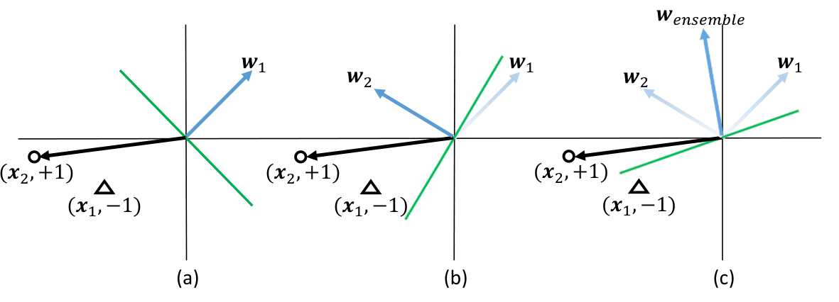
When data comes sequentially, the Perceptron algorithm makes at most $(\frac{R}{\gamma})^{2}$ mistakes (Novikoff 1963), where the margin $\gamma$ is defined as $\gamma=min_{t\in[T]|\mathbf{x}^{t}\mathbf{w}^{*}|}$ and R is a constant such that ${\forall}_{t}\in[T],\parallel\mathbf{x}_{t}\parallel\leq R$. It guarantees a tight mistake bound for online classification. But, the case in online retrieval is out of function. Essentially, online classification simply considers prediction on the current streaming data. However, for online retrieval, it has to preserve the information from the past dataset when learning from the current streaming data, since all data points are retrieved in the query stage. Therefore, directly applying Perceptron algorithm to retrieval is far from enough.

To solve it, we consider the ensemble learning to learn a weighted combination of base models from the form of

where ${\pi}^{t}$ is the tunable parameter. Empirically, we set ${\pi}^{t}=\frac{1}{T}$. That is to say, each base model obtains an equal vote on the decision of ensembled model.

Fig. 4 shows a simple example of how ensemble strategy of Eq. 42 works, the quantitative results of which are shown in Sec. 4.5. Generally, the Perceptron algorithm updates each time when a mistake occurs. However, the updated model merely absorbs the misclassified data point to ensure its correctness. As a consequence, the information from the past streaming data loses heavily. Hence, the models updated at different stages are very independent, which is infeasible in a retrieval task. The ensemble strategy to some extent integrates the independent models. Besides, since the weighted parameter ${\pi}^{t}$ is fixed, there has no much time cost to acquire $\mathbf{W}_{ensemble}$ ³³ 3 Since it is just a matrix-addition operation at each stage..

We summarize the proposed Hadamard Matrix Guided Online Hashing (HMOH) in Alg. 1⁴⁴ 4 $\tilde{W}$ is a random matrix that need not be optimized. When $r=r^{*}$, we set $\tilde{W}$ as an identity matrix.

From Alg. 1, at each updating stage, the training time is spent on kernelization of $\mathbf{X}^{t}$ in line $11$, the updating of $\mathbf{W}^{t}$ in line $12$ and the matrix addition for $\mathbf{W}_{ensemble}$ in line $13$. In line $11$, the time cost is $\mathcal{O}(n_{t}md)$. Updating $\mathbf{W}^{t}$ in line $12$ takes $\mathcal{O}(mn_{t}r^{*})$. And it also takes $\mathcal{O}(mr^{*})$ in line $13$. Above all, the total time complexity for the proposed HMOH is $\mathcal{O}(mn_{t}d+mn_{t}r^{*})$. What’s more, as experimentally demonstrated in Sec. 4.5, the suitable value of $n_{t}$ is $1$ for the proposed method. And we denote $s=\max(d,r^{*})$. Hence, without loss of generality, the overall time complexity can be further abbreviated as $\mathcal{O}(ms)$. Hence, our method is scalable.

Datasets. The CIFAR-$10$ contains $60,000$ images from $10$ classes with each class containing $6,000$ instances. Each image is represented by a $4,096$-dim feature, which is extracted from the fc7 layer of the VGG-$16$ neural network (Simonyan and Zisserman 2014) pre-trained on ImageNet (Deng et al. 2009). Following the settings in (Cakir et al. 2017b; Lin et al. 2018; Lin et al. 2019), the whole dataset is split into a retrieval set with $59K$ images and a test set with $1K$ images. Besides, we randomly sample $20K$ images from the retrieval set to form a training set to learn the hash functions.

The Places$205$ is a subset of the large-scale Places dataset (Zhou et al. 2014a) for scene recognition. It contains $2.5$ million images with each image belonging to one of the $205$ scene categories. Feature of each image is first extracted from the fc7 layer of the AlexNet (Krizhevsky et al. 2012) and then represented as a $128$-dim feature by performing PCA. To split the entire dataset, following (Lin et al. 2018), we randomly select $20$ instances from each category and the remaining is treated as the retrieval set. Lastly, a random subset of $100K$ images from the retrieval set is used to update the hash functions.

The MNIST dataset contains $70K$ handwritten digit images from $0$ to $9$. Each image is represented by $784$-dim normalized original pixels. According to the experimental settings in (Lin et al. 2019), the dataset is divided into a test set with $100$ examples randomly sampled from each class and a retrieval set with all remaining examples. $20K$ images from the retrieval set is sampled to form a training set.

The NUS-WIDE is collected from Flickr, which contains $296,648$ images. All images are manually annotated with at least one label from $81$ concepts. following (Zhou et al. 2014b; Liu et al. 2018), we preserve $186,577$ labeled images from the whole dataset according to the top $10$ frequent labels. In this dataset, each image is represented as a $500$-dim bag-of-visual-words feature. We choose $2,000$ images from this dataset as the query set, and the remaining as the retrieval set. From the retrieval set, $40$K images are randomly sampled as the training set.

Evaluation Protocols. We report the experimental results using mean Average Precision (denoted as mAP), Precision within a Hamming ball of radius $2$ centered on each query (denoted as Precision@H$2$), mAP vs. different sizes of training instances curves and their corresponding areas under the mAP curves (denoted as AUC), Precision of the top K retrieved neighbors (denoted as Precision@K) and their corresponding areas under the Precision@K curves (denoted as AUC), and Precision-Recall Curves.

Notably, when reporting the mAP performance on Places-205, following the works in (Cakir et al. 2017b; Lin et al. 2018; Lin et al. 2019), we only compute the top $1,000$ retrieved items (denoted as mAP@1,000) due to its large scale and time consumption. The above metrics are evaluated under hashing bits varying among $8$, $16$, $32$, $48$, $64$ and $128$.

Baseline Methods. We compare our method with representative state-of-the-art online hashing algorithms, including Online Kernel Hashing (OKH) (Huang et al. 2013), Online Sketching Hashing (SketchHash) (Leng et al. 2015), Adaptive Hashing (AdaptHash) (Cakir and Sclaroff 2015), Online Supervised Hashing (OSH) (Cakir et al. 2017a), Online Hashing with Mutual Information (MIHash) (Cakir et al. 2017b) and Balanced Similarity for Online Discrete Hashing (BSODH) (Lin et al. 2019). Besides, to demonstrate the advantages and improvements of the proposed HMOH, we also compare it with the previous version, i.e., HCOH (Lin et al. 2018). The public MATLAB codes of these methods are available. Our model is also implemented with MATLAB. All the experiments are performed on a server with a $3.60$GHz Intel Core I$7$ $4790$ CPU and $16$G RAM, and the experimental results are averaged over three runs.

Parametric Settings. We describe the parameters to be tuned during the experiments. Since we share the same dataset configurations on CFIAR-10, Places205 and MNIST, we directly adopt the parameters as described in (Lin et al. 2018; Lin et al. 2019), which have been carefully validated for each method. For NUS-WIDE, we also conduct careful ablation studies for all methods and set the optimal values for all the hyper-parameters. The following describes the parameter configurations for all compared baselines in details.

• •

  OKH: The tuple ($C$, $\alpha$) is set as (0.001, 0.3), (0.0001, 0.7), (0.001,0.3) and (0.001, 0.5) on CIFAR-10, Places205, MNIST and NUS-WIDE, respectively.

• •

  SketchHash: The tuple $(sketchsize,batchsize)$ is set as (200, 50), (100, 50), (200, 50) and (200, 50) on CIFAR-10, Places205, MNIST and NUS-WIDE, respectively.

• •

  AdaptHash: The tuple $(\alpha,\lambda,\eta)$ is set as (0.9, 0.01, 0.1), (0.9,0.01,0.1), (0.8, 0.01, 0.2) and (1, 0.01, 0.5) on CIFAR-10, Places205, MNIST and NUS-WIDE, respectively.

• •

  OSH: On all datasets, $\eta$ is set as $0.1$ and the ECOC codebook $C$ is populated the same way as in (Cakir et al. 2017a).

• •

  MIHash: The tuple $(\theta,\mathcal{R},A)$ is set as (0, 1000, 10), (0, 5000, 10), (0, 1000, 10) and (0, 2000, 1) on CIFAR-10, Places205, MNIST and NUS-WIDE, respectively.

• •

  BSODH: The tuple $(\lambda,\sigma,{\eta}_{s},{\eta}_{d})$ is set as (0.6, 0.5, 1.2, 0.2), (0.3, 0.5, 1.0, 0.0), (0.9, 0.8, 1.2, 0.2) and (0.3, 0.1, 0.4, 1.2) on CIFAR-10, Places205, MNIST and NUS-WIDE, respectively.

• •

  HCOH: The tuple $(n_{t},\eta)$ is set as (1, 0.2), (1, 0.1), (1, 0.2) and (1, 0.2) on CIFAR-10, Places$205$, MNIST and NUS-WIDE, respectively.

Specific descriptions of these parameters for each method can be found in (Huang et al. 2013; Leng et al. 2015; Cakir and Sclaroff 2015; Cakir et al. 2017a; Cakir et al. 2017b; Lin et al. 2019; Lin et al. 2018), respectively. As for the proposed HMOH, we list the parameter configurations on the four benchmarks in Tab. 1. Notably, experiments of the proposed method without kernelization on CIFAR-$10$ and NUS-WIDE show better results. Hence, kernel trick is not applied in the cases of CIFAR-$10$ and NUS-WIDE. Detailed analysis is conducted in Sec. 4.5.

Emphatically, for SketchHash (Leng et al. 2015), it has two limitations: First, the training size has to be larger than the code length. Second, the code length has to be smaller than the dimension of input features. Therefore, we show its experimental results with hashing bit being $8$, $16$, $32$, $48$ to follow the works in (Lin et al. 2018; Lin et al. 2019) by setting the training size as $50$. To evaluate the hashing bit of $64$ and $128$, the training size is set as $150$. In the longer code length (e.g., 256-bit and 512-bit), the experiments can not be conducted on some benchmarks due to the second limitation. All the experiments are run over three times and we report the averaged values in this paper.