跳到论文正文
W Papers独立论文阅读器 arXiv:1905.04157 论文正文 计算阅读时间 · 0%
引用这篇论文根据当前论文元数据生成,正式投稿前建议核对。


License: arXiv.org perpetual non-exclusive license
arXiv:1905.04157v2 [cond-mat.stat-mech] 22 Sep 2019

Statistics of off-diagonal entries of Wigner K−K-matrix for chaotic wave systems with absorption

Sirio Belga Fedeli    Yan V Fyodorov Affiliation: King’s College London, Department of Mathematics, London WC2R 2LS, United Kingdom
August 11, 2026
Abstract

Using the Random Matrix Theory approach we derive explicit distributions of the real and imaginary parts for off-diagonal entries of the Wigner reaction matrix 𝐊\mathbf{K} for wave chaotic scattering in systems with and without time-reversal invariance, in the presence of an arbitrary uniform absorption.

1 Introduction

The phenomenon of chaotic resonance scattering of quantum waves (or their classical analogues) has attracted considerable theoretical and experimental interest for the last three decades, see e.g. articles in [1] and recent reviews [2, 3, 4, 5]. The resonances manifest themselves via fluctuating structures in scattering observables, and understanding their statistical properties as completely as possible remains an important task. The main object in such an approach is the energy-dependent M×MM\times M random unitary scattering matrix S⁡(λ)S(\lambda), S†​(λ)​S​(λ)=𝟏MS^{\dagger}(\lambda)S(\lambda)={\bf 1}_{M} which relates amplitudes of incoming and outgoing waves at spectral parameter (energy) λ\lambda. Here the integer MM stands for the number of open channels at a given energy λ\lambda, the dagger denotes the Hermitian conjugation and 𝟏M{\bf 1}_{M} is the M×MM\times M identity matrix. Statistics of fluctuations of the scattering observables over an energy interval comparable with a typical separation between resonances can be most successfully achieved in the framework of the so called ’Heidelberg approach’ going back to the pioneering work [6], and reviewed from different perspectives in [7], [8] and [9]. In such an approach the resonance part of the SS-matrix is expressed via the Cayley transform in terms of the resolvent of a Hamiltonian 𝐇\mathbf{H} representing the closed counterpart of the scattering system as

𝐒⁡(λ)=𝟏M−i​𝐊𝟏M+i​𝐊,with𝐊=𝐖†​1λ​𝟏N−𝐇N​𝐖,\mathbf{S}(\lambda)=\frac{{\bf 1}_{M}-i\mathbf{K}}{{\bf 1}_{M}+i\mathbf{K}},\quad\hbox{with}\quad\mathbf{K}=\mathbf{W}^{\dagger}\frac{1}{\lambda{\bf 1}_{N}-\mathbf{H}_{N}}\mathbf{W}, (1)

where 𝐖\mathbf{W} is the N×MN\times M matrix containing the couplings between the channels and the system. For λ∈ℝ\lambda\in\mathbb{R}, the unitarity of 𝐒⁡(λ)\mathbf{S}(\lambda) follows from Hermiticity of the Hamiltonian represented in the framework of the Heidelberg approach by N×NN\times N self-adjoint matrix 𝐇N\mathbf{H}_{N}. The resulting M×MM\times M matrix 𝐊\mathbf{K} is known in the literature as the Wigner reaction K−K- matrix.

To study fluctuations induced by chaotic wave scattering one then follows the paradigm of relying upon the well-documented random matrix properties of the underlying Hamiltonian operator 𝐇\mathbf{H} describing quantum or wave chaotic behaviour of the closed counterpart of the scattering system. Within that approach one proceeds with replacing 𝐇N\mathbf{H}_{N} with a random matrix taken from one of the classical ensembles: Gaussian Unitary Ensemble (GUE, β=2\beta=2), if one is interested in the systems with broken time reversal invariance or Gaussian Orthogonal Ensemble (GOE, β=1\beta=1), if such invariance is preserved and no further geometric symmetries are present in the system. The columns 𝒘a,a=1,..,M\bm{w}_{a},\,\,a=1,..,M of the coupling matrix 𝐖\mathbf{W} can be considered either as fixed orthogonal vectors [6] (complex for β=2\beta=2 or real for β=1\beta=1), or alternatively as independent Gaussian-distributed random vectors orthogonal on average [10]. The results turn out to be largely insensitive to the choice of the coupling as long as inequality M≪N→∞M\ll N\to\infty holds in the calculation. The approach proved to be extremely successful, and quite a few scattering characteristics were thoroughly investigated in that framework in the last two decades, either by the variants of the supersymmetry method or related random matrix techniques, see e.g. early papers [6], [11, 12] as well as more recent results in [13, 14, 15, 16, 17]. The results of such calculations are found in general to be in good agreement with available experiments in chaotic electromagnetic resonators (“microwave billiards”), dielectric microcavities and acoustic reverberation cameras ( see reviews [2, 3, 4, 5]) as well as with numerical simulations of scattering in such paradigmatic model as quantum chaotic graphs [18] and their experimental microwave realizations [19, 20, 21, 22]. Note that the Wigner K−K-matrix is experimentally measurable in microwave scattering systems, as it is directly related to the systems impedance matrix [23, 24, 25].

One of serious challenges related to theoretical description of scattering characteristics is however related to the fact that experimentally measured quantities suffer from the inevitable energy losses (absorption), e.g. due to damping in resonator walls and other imperfections. Such losses violate unitarity of the scattering matrix and are important for interpretation of experiments, and considerable efforts were directed towards incorporating them into the Heidelberg approach [12]. At the level of the model (1) the losses can be taken into account by allowing the spectral parameter λ\lambda to have finite imaginary part by replacing λ→λ+i​α/N∈ℂ\lambda\rightarrow\lambda+i\alpha/N\in\mathbb{C} with some α>0\alpha>0. This replacement violates Hermiticity of the Wigner matrix 𝐊\mathbf{K}; in particular entries of 𝐊\mathbf{K} become now complex even for β=1\beta=1. Note that our choice of scaling of the absorption term with NN is to ensure access to the most interesting, difficult and experimentally relevant regime when absorption term is comparable with the mean separation between neighbouring eigenvalues of the wave-chaotic Hamiltonian HH, the latter being in the chosen normalization of the order N−1N^{-1} as N→∞N\to\infty. The statistics of the real and imaginary parts of the diagonal entries 𝐊a​a{\bf K}_{aa} in that regime was subject of considerable theoretical work [26, 27, 28] and by now well-understood and measured experimentally with good precision for β=1\beta=1 in microwave cavities [29, 23, 24, 25] and graphs [19, 20, 21, 22]. Very recently first experimental results for β=2\beta=2 were reported as well [30].

The situation with off-diagonal elements 𝐊a≠b\mathbf{K}_{a\neq b} is in comparison much worse. At present no theoretical results for the associated distributions are available in the literature for the most interesting and experimentally relevant case β=1\beta=1 apart from the case of zero absorption [15], and the mean value and variance for |𝐊a​b|2=(ℑ⁡𝐊a≠b)2+(ℜ⁡𝐊a≠b)2|\mathbf{K}_{ab}|^{2}=(\Im\mathbf{K}_{a\neq b})^{2}+(\Re\mathbf{K}_{a\neq b})^{2} [31]. The main goal of the present paper is to fill in this gap partly by presenting the distribution of imaginary ℑ⁡𝐊a≠b\Im\mathbf{K}_{a\neq b} and real ℜ⁡𝐊a≠b\Re\mathbf{K}_{a\neq b} parts for the K−K-matrix entries in the presence of absorption:

𝐊a,b=Tr⁡{((λ+i​αN)​𝟏N−𝐇N)−1​𝒘b⊗𝒘aT}\mathbf{K}_{a,b}=\Tr\Bigg\{\Big(\left(\lambda+i\frac{\alpha}{N}\right){\bf 1}_{N}-\mathbf{H}_{N}\Big)^{-1}\bm{w}_{b}\otimes\bm{w}_{a}^{T}\Bigg\} (2)

for systems with preserved (β=1\beta=1) time reversal invariance, assuming the size N→∞N\to\infty. Our method also straightforwardly works for the simpler case of broken time-reversal invariance (β=2\beta=2) where the full distribution of |Ka≠b|2|K_{a\neq b}|^{2} has in fact already been derived for the case of uncorrelated channels, see eqs.(11)-(13) in [32]. We start with briefly reconsidering that case in our framework, giving an alternative derivation of the result in [32], and showing that it is simply related to the joint probability density of ℑ⁡𝐊a≠b\Im\mathbf{K}_{a\neq b} and ℜ⁡𝐊a≠b\Re\mathbf{K}_{a\neq b}. We then provide a generalization of that result to the case of correlated channel vectors, see Eq.(8). Then we concentrate on the β=1\beta=1 case.

2 Discussion of the main results

2.1 Systems with broken time-reversal invariance

In this case we assume that the matrix 𝐇N\mathbf{H}_{N} is a complex Hermitian GUE matrix distributed according to the probabilty density d𝒫(𝐇N)∝e−N/2Tr𝐇N𝐇N†d𝐇Nd\mathcal{P}(\mathbf{H}_{N})\propto e^{-N/2\Tr\mathbf{H}_{N}\mathbf{H}_{N}^{{\dagger}}}d\mathbf{H}_{N}, so that the expectations over the ensemble are defined by ⟨[…]⟩G​U​E​(N):=∫[…]​𝑑𝒫​(𝐇N)\langle[...]\rangle_{GUE(N)}:=\int[...]d\mathcal{P}(\mathbf{H}_{N}). Initially we assume for simplicity that the components of the channel vectors 𝒘a\bm{w}_{a} and 𝒘b\bm{w}_{b} are uncorrelated complex gaussian random variables with mean zero and variance 1/N1/N, and we denote the expectation values with respect to the channel vectors by the overbar. Next, we consider the simplest nontrivial case of correlated channels characterized by a 2×22\times 2 covariance matrix. Note that to compute the joint probabilty density of real and imaginary parts of 𝐊a,b\mathbf{K}_{a,b} it is technically more convenient to consider its characteristic function, given by the Fourier transform

ℛ⁡(q,q∗)=⟨exp⁡i/2​(q​𝐊a,b∗+q∗​𝐊a,b)⟩¯G​U​E​(N).\mathcal{R}(q,q^{*})=\overline{\langle\exp{i/2(q\mathbf{K}_{a,b}^{*}+q^{*}\mathbf{K}_{a,b})}\rangle}_{GUE(N)}. (3)

2.1.1 Uncorrelated channel vectors 𝒘a\bm{w}_{a} and 𝒘b\bm{w}_{b}.

The complex gaussian nature of components of the channel vectors 𝒘a\bm{w}_{a} allows one to easily relate the characteristic function (3) to the GUE expectation of ratios of characteristic polynomials (for the derivation see Sec. (3.1) below):

ℛ⁡(q,q∗)=⟨det((𝐇N−λ​𝟏N)2+α2N2​𝟏N)det((𝐇N−λ​𝟏N)2+α2+|q/2|2N2​𝟏N)⟩G​U​E​(N)\mathcal{R}(q,q^{*})=\Bigg\langle\frac{\det\left((\mathbf{H}_{N}-\lambda{\bf 1}_{N})^{2}+\frac{\alpha^{2}}{N^{2}}{\bf 1}_{N}\right)}{\det\left((\mathbf{H}_{N}-\lambda{\bf 1}_{N})^{2}+\frac{\alpha^{2}+|q/2|^{2}}{N^{2}}{\bf 1}_{N}\right)}\Bigg\rangle_{GUE(N)} (4)

The expectation values of products of ratios of characteristic polynomials (and their large−N-N asymptotics) are well known, see [33, 34, 35]. Using those results one easily obtains the following expression for ℛ⁡(q,q∗)≡ℛ⁡(|q|)\mathcal{R}(q,q^{*})\equiv\mathcal{R}(|q|) in the limit N→∞N\rightarrow\infty for any value λ\lambda of the spectral parameter belonging to the bulk of the GUE spectrum:

ℛ⁡(|q|)=|q/2|4​exp⁡(−2​π​ρ​(λ)​α2+|q/2|2)4​α​α2+|q/2|2\mathcal{R}(|q|)=\frac{|q/2|^{4}\exp{(-2\pi\rho(\lambda)\sqrt{\alpha^{2}+|q/2|^{2}})}}{4\alpha\sqrt{\alpha^{2}+|q/2|^{2}}} (5)
×(exp⁡(2​π​ρ​(λ)​α)(α2+|q/2|2−α)2−exp⁡(−2​π​ρ​(λ)​α)(α2+|q/2|2+α)2),,λ∈(−2,2)\times\Bigg(\frac{\exp{(2\pi\rho(\lambda)\alpha)}}{(\sqrt{\alpha^{2}+|q/2|^{2}}-\alpha)^{2}}-\frac{\exp{(-2\pi\rho(\lambda)\alpha)}}{(\sqrt{\alpha^{2}+|q/2|^{2}}+\alpha)^{2}}\Bigg),\quad,\lambda\in(-2,2)

where ρ⁡(λ)=1/(2​π)​4−λ2\rho(\lambda)=1/(2\pi)\sqrt{4-\lambda^{2}} is the mean density of GUE eigenvalues given by the Wigner semicircular law. The numerical verification of (5) for systems with broken time-reversal symmetry is provided in Fig. 1 below.

Inverting this characteristic function yields the joint probability density function of 𝐊a,b\mathbf{K}_{a,b} and 𝐊a,b∗\mathbf{K}_{a,b}^{*} described in the following

Proposition 1: Define the operator 𝒟x^\hat{\mathcal{D}_{x}} as

𝒟^x=sinh⁡(x)​(1+d2d​x2)−2​cosh⁡(x)​dd​x\hat{\mathcal{D}}_{x}=\sinh(x)\Big(1+\frac{d^{2}}{dx^{2}}\Big)-2\cosh(x)\frac{d}{dx}

Then the joint probability density function of the pair (𝐊a​b,𝐊a​b∗)(\mathbf{K}_{ab},\mathbf{K}_{ab}^{*}), with 𝐇N∈G​U​E​(N)\mathbf{H}_{N}\in GUE(N) in the limit N→∞N\rightarrow\infty is given by:

𝒫⁡(𝐊a,b,𝐊a,b∗)=α2π​limx→2​π​ρ​(λ)​α𝒟^x​exp⁡(−x2+4​α2​|𝐊a,b|2)x2+4​α2​|𝐊a,b|2\mathcal{P}(\mathbf{K}_{a,b},\mathbf{K}_{a,b}^{*})=\frac{\alpha^{2}}{\pi}\lim_{x\rightarrow 2\pi\rho(\lambda)\alpha}\hat{\mathcal{D}}_{x}\frac{\exp{(-\sqrt{x^{2}+4\alpha^{2}|\mathbf{K}_{a,b}|^{2}})}}{\sqrt{x^{2}+4\alpha^{2}|\mathbf{K}_{a,b}|^{2}}} (6)
Refer to caption
Refer to caption
Figure 1: Characteristic function Eq.(5) for systems with broken time-reversal invariance for α=1​(b​l​u​e),α=5​(r​e​d),α=10​(y​e​l​l​o​w)\alpha=1(blue),\,\alpha=5(red),\,\alpha=10(yellow) and λ=0​(t​o​p),λ=1​(b​o​t​t​o​m)\lambda=0(top),\,\lambda=1(bottom) versus direct numerical simulations (# N=100N=100, 50000 samples, circular markers).

In the case α→0+\alpha\rightarrow 0^{+}, which corresponds to vanishing absorption, the joint density 𝒫⁡(𝐊a,b,𝐊a,b∗)\mathcal{P}(\mathbf{K}_{a,b},\mathbf{K}_{a,b}^{*}) acquires a simple form:

𝒫⁡(ℜ⁡𝐊a,b,ℑ⁡𝐊a,b)=ρ⁡(λ)4​|𝐊a,b|2+4​π2​ρ2​(λ)(|𝐊a,b|2+π2​ρ2​(λ))5/2\mathcal{P}\left(\Re\mathbf{K}_{a,b},\Im\mathbf{K}_{a,b}\right)=\frac{\rho(\lambda)}{4}\frac{|\mathbf{K}_{a,b}|^{2}+4\pi^{2}\rho^{2}(\lambda)}{(|\mathbf{K}_{a,b}|^{2}+\pi^{2}\rho^{2}(\lambda))^{5/2}}

which implies due to the rotational symmetry that the variables u1=ℜ⁡𝐊a,bu_{1}=\Re\mathbf{K}_{a,b} and u2=ℑ⁡𝐊a,bu_{2}=\Im\mathbf{K}_{a,b} each are distributed, respectively, as:

𝒫(ui)=ρ⁡(λ)2ui2+3​π2​ρ2​(λ)(ui2+π2​ρ2​(λ))2,i=1,2\mathcal{P}(u_{i})=\frac{\rho(\lambda)}{2}\frac{u_{i}^{2}+3\pi^{2}\rho^{2}(\lambda)}{(u_{i}^{2}+\pi^{2}\rho^{2}(\lambda))^{2}},\quad i=1,2

Note that the results for arbitrary spectral parameter λ∈(−2,2)\lambda\in(-2,2) could be obtained from those for λ=0\lambda=0 by rescaling α→α​η\alpha\rightarrow\alpha\eta and |q|→|q|​η|q|\rightarrow|q|\eta with the ratio η=ρ⁡(λ)/ρ⁡(0)\eta=\rho(\lambda)/\rho(0). This is a particular manifestation of the well-known spectral universality of random matrix results, the property which we will use in the next section to deal with a much more challenging problem of scattering systems with preserved time-reversal invariance.

2.1.2 Correlated channel vectors 𝒘a\bm{w}_{a} and 𝒘b\bm{w}_{b}.

To consider the simplest nontrivial correlations between channel vectors we assume that the entries wa,nw_{a,n} (resp. wb,nw_{b,n}) with different values of nn remain independent and identically distributed gaussian variables, whereas wa,nw_{a,n} and wb,nw_{b,n} with the same value of nn are correlated. The correlations can be then described by a non-diagonal 2×22\times 2 Hermitian positive definite covariance matrix 𝐂−𝟏\mathbf{C^{-1}} such that 𝒘a†​𝒘b¯=(C−1)a​b\overline{\bm{w}_{a}^{\dagger}\bm{w}_{b}}=\left(C^{-1}\right)_{ab}. The corresponding joint probability density 𝒫⁡(wa,n,wb,n)\mathcal{P}\left(w_{a,n},w_{b,n}\right) has the form

𝒫⁡(wa,n,wb,n)∝exp⁡{−N​[wa,nwb,n]†​𝐂​[wa,nwb,n]}\mathcal{P}\left(w_{a,n},w_{b,n}\right)\propto\exp\Big\{-N\left[\begin{array}[]{c}w_{a,n}\\ w_{b,n}\\ \end{array}\right]^{{\dagger}}\mathbf{C}\left[\begin{array}[]{c}w_{a,n}\\ w_{b,n}\\ \end{array}\right]\Big\}

It is then easy to show that the resulting characteristic function is again expressed as the ratio of determinants, similar to the uncorrelated case:

ℛ⁡(q,q∗)=⟨det((λ​𝟏N−𝐇N)2+α2N2​𝟏N)Πl=1,2​det((λ​𝟏N−𝐇N)+i2​N​(k~+(−1)l​k~2+4​s~)​𝟏N)⟩G​U​E​(N),\mathcal{R}(q,q^{*})=\Bigg\langle\frac{\det\left((\lambda{\bf 1}_{N}-\mathbf{H}_{N})^{2}+\frac{\alpha^{2}}{N^{2}}{\bf 1}_{N}\right)}{\Pi_{l=1,2}\det\left((\lambda{\bf 1}_{N}-\mathbf{H}_{N})+\frac{i}{2N}(\tilde{k}+(-1)^{l}\sqrt{\tilde{k}^{2}+4\tilde{s}}){\bf 1}_{N}\right)}\Bigg\rangle_{GUE(N)}, (7)

where we denoted:

k~=12​(Ca​b∗det𝐂​q+Ca​bdet𝐂​q∗)\tilde{k}=\frac{1}{2}\Big(\frac{C_{ab}^{*}}{\det\mathbf{C}}q+\frac{C_{ab}}{\det\mathbf{C}}q^{*}\Big)
s~=α2+α2​(Ca​b∗det𝐂​q−Ca​bdet𝐂​q∗)+|q|24​det𝐂\tilde{s}=\alpha^{2}+\frac{\alpha}{2}\Big(\frac{C_{ab}^{*}}{\det\mathbf{C}}q-\frac{C_{ab}}{\det\mathbf{C}}q^{*}\Big)+\frac{|q|^{2}}{4\det{\mathbf{C}}}

It is useful to recall that Ca​bdet𝐂=−(C−1)a​b\frac{C_{ab}}{\det\mathbf{C}}=-\left(C^{-1}\right)_{ab} so reflects the nonvanishing correlations between the two channel vectors.

Note that we assume the entries of 𝐂\mathbf{C} to be of order unity: Ci,j=a,b=O⁡(1)C_{i,j=a,b}=O(1) as N→∞N\to\infty. Evaluating then the expectation over the GUE matrices in (7), we find in the large-NN limit:

ℛ⁡(q,q∗)=e−12​(i​k~​λ)−π​ρ​(λ)​(k~2+4​s~+2​α)8​(k~2+4​s~)​α​((1−e4​π​α​ρ​(λ))​k~2−(k~2+4​s~−2​α)2+e4​π​α​ρ​(λ)​(k~2+4​s~+2​α)2)\mathcal{R}(q,q^{*})=\frac{e^{-\frac{1}{2}(i\tilde{k}\lambda)-\pi\rho(\lambda)(\sqrt{\tilde{k}^{2}+4\tilde{s}}+2\alpha)}}{8(\sqrt{\tilde{k}^{2}+4\tilde{s}})\alpha}\Big((1-e^{4\pi\alpha\rho(\lambda)})\tilde{k}^{2}-(\sqrt{\tilde{k}^{2}+4\tilde{s}}-2\alpha)^{2}+e^{4\pi\alpha\rho(\lambda)}(\sqrt{\tilde{k}^{2}+4\tilde{s}}+2\alpha)^{2}\Big) (8)

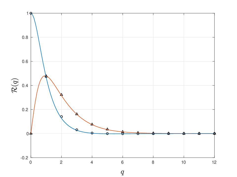
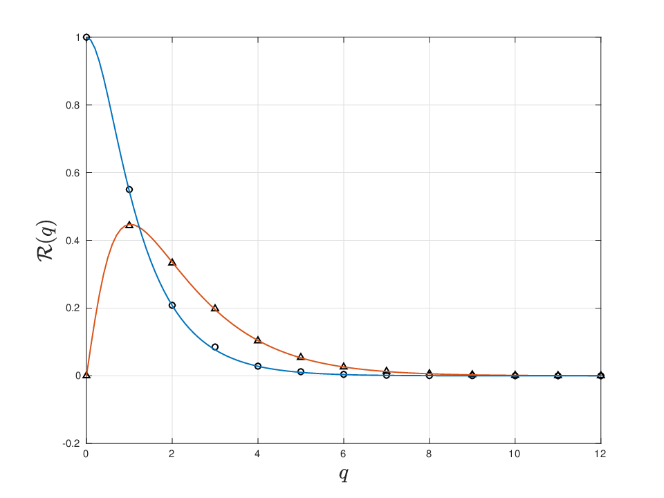
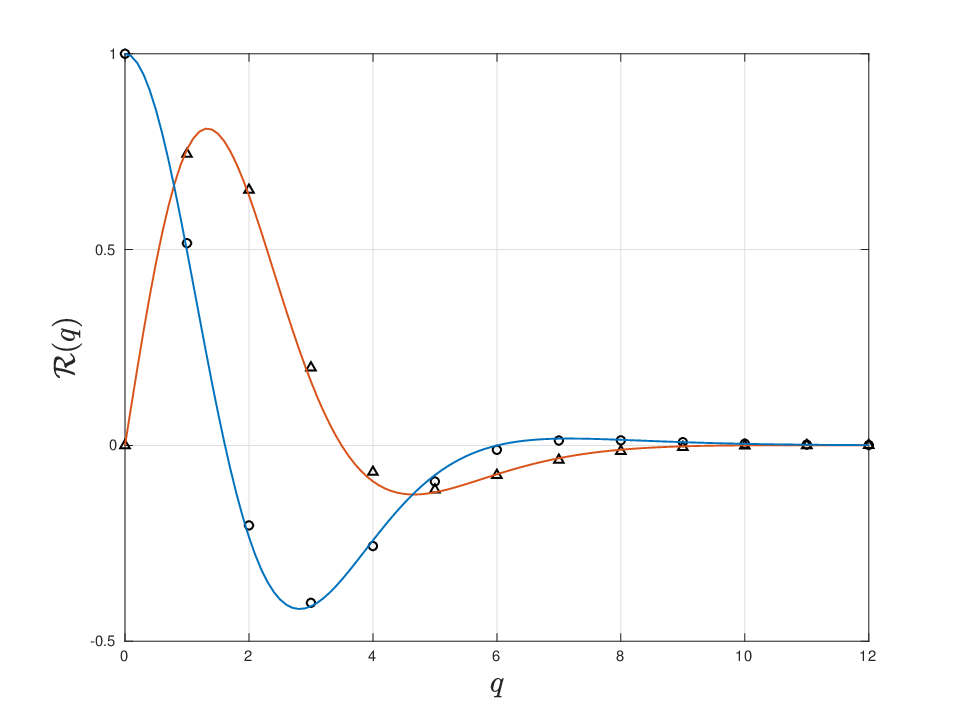
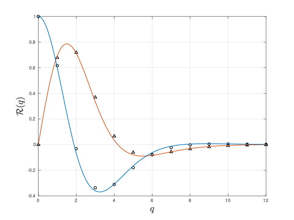
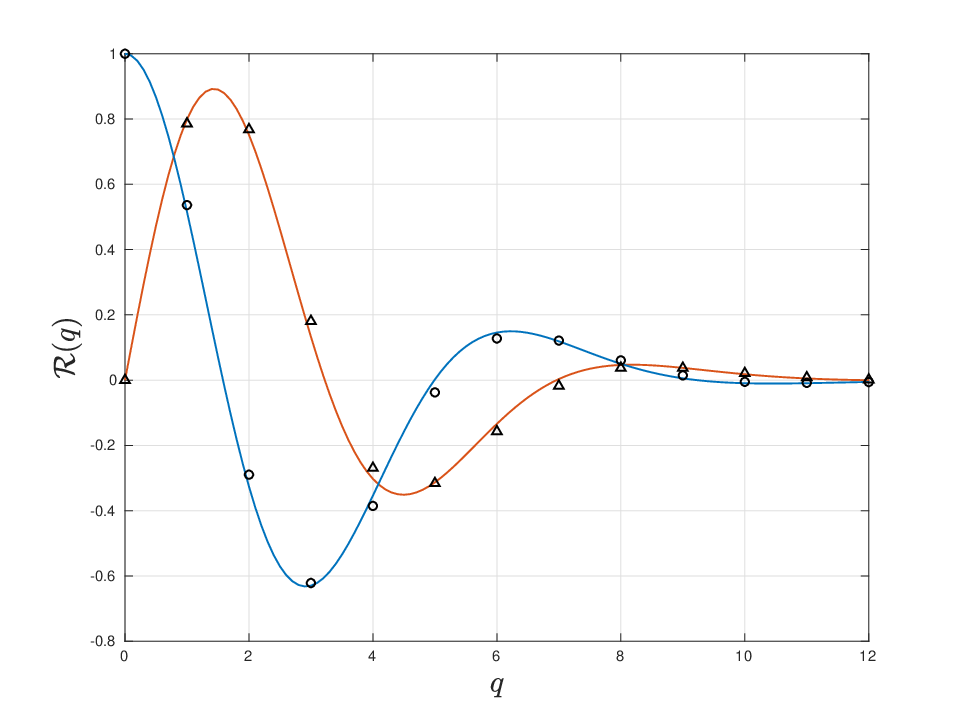
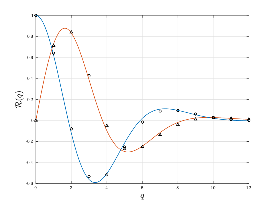
Examples of ℛ⁡(q,q∗)\mathcal{R}(q,q^{*}) for different levels of absorption are shown in Fig. 2, Fig. 3 and Fig.4 for a particular choice of the covariance matrix 𝐂−1=[2−ii1]\mathbf{C}^{-1}=\left[\begin{array}[]{cc}2&-i\\ i&1\\ \end{array}\right]. Small discrepancies between simulations and the theoretical formula visible in the figures are due to the finite size of the matrices used in simulations and can be checked to gradually disappear as the size of the matrices is increased. The latter effect is the more pronounced the bigger values of α\alpha are considered.

Refer to caption
Refer to caption
Figure 2: Real (blue) and imaginary (red) parts of the characteristic function Eq.(8) for Ka,bK_{a,b} in systems with broken time-reversal invariance and absorption α=1\alpha=1 with the special choice of the channel covariance matrix, for λ=0\lambda=0 (top),λ=1\lambda=1 (bottom). Markers indicate numerical results involving # Samples 10000 for the matrix size NN=100.
Refer to caption
Refer to caption
Figure 3: The same as above for absorption α=5\alpha=5
Refer to caption
Refer to caption
Figure 4: The same as above for absorption α=10\alpha=10.

2.2 Systems with preseved time-reversal invariance

In such a case we assume 𝐇N\mathbf{H}_{N} to be the real symmetric GOE matrix distributed with the probability density d​𝒫​(𝐇N)∝exp⁡(−N4​Tr⁡𝐇N2)​d​𝐇Nd\mathcal{P}(\mathbf{H}_{N})\propto\exp(-\frac{N}{4}\Tr\mathbf{H}_{N}^{2})d\mathbf{H}_{N}, whereas the channel vectors 𝒘a\bm{w}_{a} are assumed to be independent for a≠ba\neq b and their components are chosen to be real i.i.d. mean-zero gaussian random variables of variance Var[𝒘a​j]=1/N,j=1…,NVar[\bm{w}_{aj}]=1/N,\,j=1\ldots,N. In what follows we denote the corresponding expectations with […]¯=∫∫⁡[…]​𝒫​(𝒘a)​𝒫​(𝒘b)​d​𝒘a​d​𝒘b\overline{[...]}=\int\int[...]\mathcal{P}(\bm{w}_{a})\mathcal{P}(\bm{w}_{b})d\bm{w}_{a}d\bm{w}_{b} and ⟨[…]⟩G​O​E​(N)=∫[…]​𝒫​(𝐇N)​d​𝐇N\langle[...]\rangle_{GOE(N)}=\int[...]\mathcal{P}(\mathbf{H}_{N})d\mathbf{H}_{N} respectively. As before, to address the distributions of 𝐊a,b=ℜ⁡𝐊a,b+i​ℑ⁡𝐊a,b\mathbf{K}_{a,b}=\Re\mathbf{K}_{a,b}+i\Im\mathbf{K}_{a,b} we introduce its characteristic function ℛ⁡(k,s),q=k+i​s\mathcal{R}(k,s),q=k+is as in (3). Integrating out the Gaussian-distributed channel vectors one arrives at the following representation:

ℛ⁡(k,s)=⟨det((λ​𝟏N−𝐇N)2+α2N2​𝟏N)Πl=1,2​det1/2((λ​𝟏N−𝐇N)2+(−1)l​i​kN​(λ​𝟏N−𝐇N)+ωl2N2​𝟏N)⟩G​O​E​(N),\mathcal{R}(k,s)=\Bigg\langle\frac{\det\left((\lambda{\bf 1}_{N}-\mathbf{H}_{N})^{2}+\frac{\alpha^{2}}{N^{2}}{\bf 1}_{N}\right)}{\Pi_{l=1,2}\det^{1/2}\left((\lambda{\bf 1}_{N}-\mathbf{H}_{N})^{2}+(-1)^{l}i\frac{k}{N}(\lambda{\bf 1}_{N}-\mathbf{H}_{N})+\frac{\omega_{l}^{2}}{N^{2}}{\bf 1}_{N}\right)}\Bigg\rangle_{GOE(N)}, (9)

where we denoted ω12=α2−i​α​s\omega_{1}^{2}=\alpha^{2}-i\alpha s and ω22=α2+i​α​s\omega_{2}^{2}=\alpha^{2}+i\alpha s.

The major difficulties in evaluating such type of GOE averages arise from the presence of half-integer powers in the denominator. Using a variant of the supersymmtry approach one can derive a finite−N-N representation for the above as an integral over 4×44\times 4 positive definite matrices (see Appendix A), but its asymptotic/saddle-point analysis for N≫1N\gg 1 presents a considerable technical challenge, see a detailed discussion in [15]. Note also the lack of rotational invariance in the plane of the complex variable qq as, in contrast to the GUE case, ℛ⁡(k,s)\mathcal{R}(k,s) does not depend only on |q|=k2+s2|q|=\sqrt{k^{2}+s^{2}} . Athough all this prevented us from finding the full joint probability density for the pair (𝐊a,b,𝐊a,b∗)(\mathbf{K}_{a,b},\mathbf{K}_{a,b}^{*}), we succeeded in extracting the (most important) special cases:

ℛ⁡(s,0)=⟨exp⁡(i​s​ℑ⁡𝐊a,b)¯⟩G​O​E​(N),ℛ⁡(0,k)=⟨exp⁡(i​k​ℜ⁡𝐊a,b)¯⟩G​O​E​(N)\mathcal{R}(s,0)=\langle\overline{\exp{\left(is\Im{\mathbf{K}_{a,b}}\right)}}\rangle_{GOE(N)},\quad\mathcal{R}(0,k)=\langle\overline{\exp{\left(ik\Re{\mathbf{K}_{a,b}}\right)}}\rangle_{GOE(N)} (10)

yielding the characteristic function for separately imaginary and real part of 𝐊a,b\mathbf{K}_{a,b}. Note that those quantities can be separately measured. To simplify our calculation we concentrate on the spectral centre λ=0\lambda=0, the general case λ≠0\lambda\neq 0 recovered by using the spectral universality via rescaling with the mean spectral density, exactly like in β=2\beta=2 case. Our main result for the characteristic functions is given by

Proposition 2: Consider 𝐇N∈G​O​E​(N)\mathbf{H}_{N}\in GOE(N), 𝐰c∼𝒩⁡(𝟎,1N​𝟏N)\bm{w}_{c}\sim\mathcal{N}(\bm{0},\frac{1}{N}{\bf 1}_{N}) for c=a,bc=a,b and define the functions

C⁡(q1,q2,α)=q22−4​q23+4​q13​(4​q2−1)+2​q1​q2​(1−4​q2+8​q22)+q12​(1−8​q2+44​q22)C(q_{1},q_{2},\alpha)=q_{2}^{2}-4q_{2}^{3}+4q_{1}^{3}(4q_{2}-1)+2q_{1}q_{2}(1-4q_{2}+8q_{2}^{2})+q_{1}^{2}(1-8q_{2}+44q_{2}^{2}) (11)
−4​(q1+q2)​(−q23+q12​q2​(4​q2−5)+q1​q22​(4​q2−5)+q13​(4​q2−1))​α2+16​q12​q22​(q1+q2)2​α4-4(q_{1}+q_{2})\left(-q_{2}^{3}+q_{1}^{2}q_{2}(4q_{2}-5)+q_{1}q_{2}^{2}(4q_{2}-5)+q_{1}^{3}(4q_{2}-1)\right)\alpha^{2}+16q_{1}^{2}q_{2}^{2}(q_{1}+q_{2})^{2}\alpha^{4}

and

D⁡(q1,q2,α)=C⁡(q1,q2,α)−8​(q1+q2)2​α2​(q1+q2−2​q1​q2+4​q1​q2​(q1+q2)​α2)D(q_{1},q_{2},\alpha)=C(q_{1},q_{2},\alpha)-8(q_{1}+q_{2})^{2}\alpha^{2}\left(q_{1}+q_{2}-2q_{1}q_{2}+4q_{1}q_{2}(q_{1}+q_{2})\alpha^{2}\right) (12)

Then the characteristic function of the real ℜ\Re and imaginary ℑ\Im parts of 𝐊a​b\mathbf{K}_{ab} for λ=0\lambda=0 are given in the limit N→∞N\to\infty by the following integral representations:

limN→∞⟨ei​s​ℑ⁡𝐊a,b⟩¯G​O​E​(N)=−∫ℝ+dq1∫ℝ+dq2|q1−q2|J0(sα(q1−q2))\lim_{N\rightarrow\infty}\overline{\Big\langle{e^{is\Im\mathbf{K}_{a,b}}}\Big\rangle}_{GOE(N)}=-\int_{\mathbb{R}_{+}}dq_{1}\int_{\mathbb{R}_{+}}dq_{2}|q_{1}-q_{2}|J_{0}\Big(s\alpha(q_{1}-q_{2})\Big)
×e−14​(q1+q2)​((q1​q2)−1+4​α2)​D⁡(q1,q2,α)​sinh⁡(2​α)−2​α​C​(q1,q2,α)​cosh⁡(2​α)512​π​q13​q23​(q1+q2)5/2​α3\times\,\,e^{-\frac{1}{4}(q_{1}+q_{2})\left((q_{1}q_{2})^{-1}+4\alpha^{2}\right)}\,\,\frac{D(q_{1},q_{2},\alpha)\sinh(2\alpha)-2\alpha C(q_{1},q_{2},\alpha)\cosh(2\alpha)}{512\sqrt{\pi}q_{1}^{3}q_{2}^{3}(q_{1}+q_{2})^{5/2}\alpha^{3}} (13)

and

limN→∞⟨ei​k​ℜ⁡𝐊a,b⟩¯G​O​E​(N)=−∫ℝ+dq1∫ℝ+dq1dq2|q1−q2|I0(kk24+α2(q1−q2))\lim_{N\rightarrow\infty}\overline{\Big\langle{e^{ik\Re\mathbf{K}_{a,b}}}\Big\rangle}_{GOE(N)}=-\int_{\mathbb{R}_{+}}dq_{1}\int_{\mathbb{R}_{+}}dq_{1}dq_{2}|q_{1}-q_{2}|I_{0}\Big(k\sqrt{\frac{k^{2}}{4}+\alpha^{2}}(q_{1}-q_{2})\Big)
×e−14​(q1+q2)​((q1​q2)−1+2​(k2+2​α2))​D⁡(q1,q2,α)​sinh⁡(2​α)−2​α​C​(q1,q2,α)​cosh⁡(2​α)512​π​q13​q23​(q1+q2)5/2​α3\times\,\,e^{-\frac{1}{4}(q_{1}+q_{2})\left((q_{1}q_{2})^{-1}+2(k^{2}+2\alpha^{2})\right)}\,\,\frac{D(q_{1},q_{2},\alpha)\sinh(2\alpha)-2\alpha C(q_{1},q_{2},\alpha)\cosh(2\alpha)}{512\sqrt{\pi}q_{1}^{3}q_{2}^{3}(q_{1}+q_{2})^{5/2}\alpha^{3}} (14)

where J0​(x)J_{0}(x) and I0​(x)I_{0}(x) are Bessel function and modified Bessel function, respectively.

Note 1. The probability density function of the scaled imaginary part u=α−1​ℑ⁡Ka​bu=\alpha^{-1}\Im K_{ab} can be written in a closed form by inverting the associated Fourier transform. Namely, denoting the integrand function in equation (13) for s=0s=0 as f⁡(q1,q2,α)f(q_{1},q_{2};\alpha) one gets

𝒫⁡(u)=∫01∫01d​p​𝑑t​f​(|u|(2​p​t)​(t+1),|u|(2​p​t)​(1−t),α)​|u|p2​t2​1−p2\mathcal{P}(u)=\int_{0}^{1}\int_{0}^{1}dpdtf\Big(\frac{|u|}{(2pt)}(t+1),\frac{|u|}{(2pt)}(1-t);\alpha\Big)\frac{|u|}{p^{2}t^{2}\sqrt{1-p^{2}}} (15)

A similar inversion in (14) seems however impractical.

Note 2. Introduce the GOE semicircle eigenvalue density ρ⁡(λ)=1/(2​π)​4−λ2\rho(\lambda)=1/(2\pi)\sqrt{4-\lambda^{2}} and the ratio η=ρ⁡(λ)/ρ⁡(0)\eta=\rho(\lambda)/\rho(0). Then characteristic functions ⟨exp⁡(i​s​ℑ⁡𝐊a,b)¯⟩G​O​E​(N)\langle\overline{\exp{\left(is\Im\mathbf{K}_{a,b}\right)}}\rangle_{GOE(N)} and ⟨exp⁡(i​k​ℜ⁡𝐊a,b)¯⟩G​O​E​(N)\langle\overline{\exp{\left(ik\Re\mathbf{K}_{a,b}\right)}}\rangle_{GOE(N)} for any λ∈(−2,2)\lambda\in(-2,2) in the limit N→∞N\rightarrow\infty can be obtained from the case λ=0\lambda=0 by rescalings α→η​α\alpha\rightarrow\eta\alpha, s→η​ss\rightarrow\eta s and k→η​kk\rightarrow\eta k. Namely:

limN→∞⟨ei​s​ℑ⁡𝐊a,b⟩¯G​O​E​(N)​(α,λ)=limN→∞⟨ei​s​η​ℑ⁡𝐊a,b⟩¯G​O​E​(N)​(η​α,0)\lim_{N\rightarrow\infty}\overline{\Big\langle e^{{is\Im\mathbf{K}_{a,b}}}\Big\rangle}_{GOE(N)}(\alpha,\lambda)=\lim_{N\rightarrow\infty}\overline{\Big\langle e^{{is\eta\Im\mathbf{K}_{a,b}}}\Big\rangle}_{GOE(N)}(\eta\alpha,0) (16)

and

limN→∞⟨ei​k​ℜ⁡𝐊a,b⟩¯G​O​E​(N)​(α,λ)=limN→∞⟨ei​k​η​ℜ⁡𝐊a,b⟩¯G​O​E​(N)​(η​α,0)\lim_{N\rightarrow\infty}\overline{\Big\langle e^{{ik\Re\mathbf{K}_{a,b}}}\Big\rangle}_{GOE(N)}(\alpha,\lambda)=\lim_{N\rightarrow\infty}\overline{\Big\langle e^{{ik\eta\Re\mathbf{K}_{a,b}}}\Big\rangle}_{GOE(N)}(\eta\alpha,0) (17)

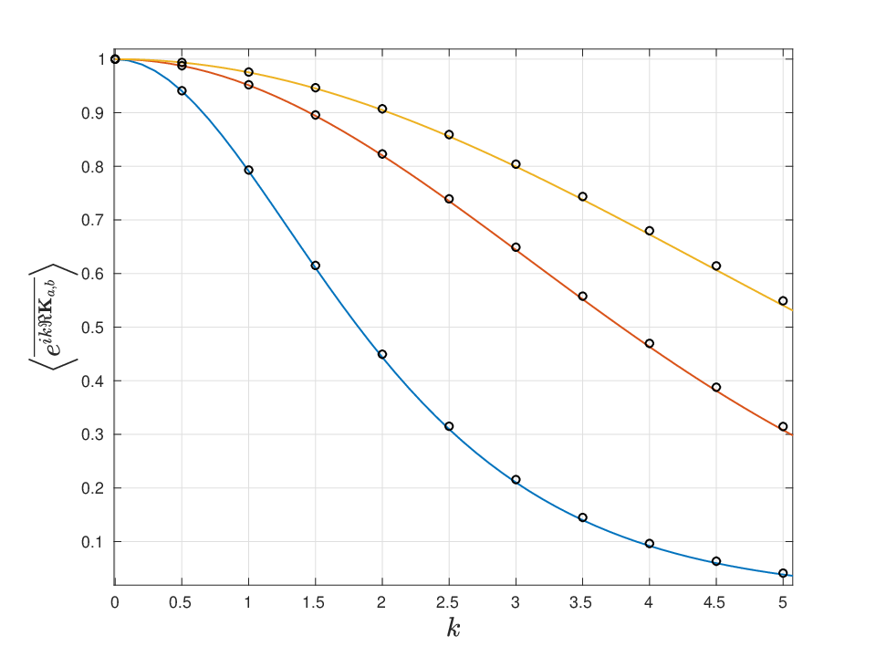
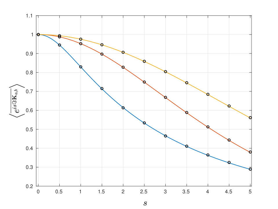
An analogous result holds for the probability distribution 𝒫⁡(⋅,α,λ)\mathcal{P}(\cdot;\alpha,\lambda) in eq. (15) with λ≠0\lambda\neq 0; now rescaling u~=η2​u\tilde{u}=\eta^{2}u, i.e. 𝒫⁡(u~,ε,λ)=𝒫⁡(u~,η​α,0)\mathcal{P}(\tilde{u};\varepsilon,\lambda)=\mathcal{P}(\tilde{u};\eta\alpha,0). The numerical comparison is presented in Figs. 2 and 3 below. A justification for the rescaling can been provided based on the results in [15], see appendix A.

Note 3. For large values of absorption α≫1\alpha\gg 1 it is natural to expect that the probability density of ℑ⁡𝐊a,b\Im\mathbf{K}_{a,b} should approach the Gaussian shape. This is fully confirmed by Fig. 4.

Note 4. Although we were not able to find the joint probability density for the pair ℜ⁡𝐊a,b\Re\mathbf{K}_{a,b} and ℑ⁡𝐊a,b\Im\mathbf{K}_{a,b}, we can shed some light on cross-correlations between the imaginary and real parts by using the results of the paper [31] for the variance of |𝐊a​b|2=(ℑ⁡𝐊a≠b)2+(ℜ⁡𝐊a≠b)2|\mathbf{K}_{ab}|^{2}=(\Im\mathbf{K}_{a\neq b})^{2}+(\Re\mathbf{K}_{a\neq b})^{2}. Namely, in Fig. 5 we present the quantity

τ⁡(α)=⟨(ℑ⁡Ka,b​ℜ⁡Ka,b)2⟩¯⟨(ℑ⁡Ka,b)2⟩¯⟨(ℜ⁡Ka,b)2⟩¯−1,\tau(\alpha)=\frac{\overline{\langle\left(\Im K_{a,b}\Re K_{a,b}\right)^{2}\rangle}}{\overline{\langle\left(\Im K_{a,b}\right)^{2}\rangle}\quad\overline{\langle\left(\Re K_{a,b}\right)^{2}\rangle}}-1,

where ⟨(ℑ⁡Ka,b)2⟩¯\overline{\langle\left(\Im K_{a,b}\right)^{2}\rangle} and ⟨(ℜ⁡Ka,b)2⟩¯\overline{\langle\left(\Re K_{a,b}\right)^{2}\rangle} are calculated in the Appendix B. We see that the real and imaginary parts are correlated, but gradually decorrelate with increased absorption.

Acknowledgments: The research presented in this paper was supported by EPSRC grant EP/N009436/1 ”The many faces of random characteristic polynomials” and by the EPSRC Centre for Doctoral Training in Cross-Disciplinary Approaches to Non-Equilibrium Systems (CANES, EP/L015854/1)
Refer to caption
Refer to caption
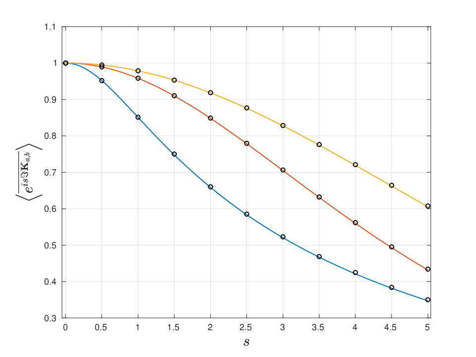
Figure 5: Characteristic function of ℑ⁡Ka,b\Im K_{a,b} as given by (13) vs. numerical simulations for systems with preserved time-reversal invariance at different level of absorption: α=1​(b​l​u​e),5​(r​e​d),10​(y​e​l​l​o​w)\alpha=1(blue),5(red),10(yellow) (# Samples 80000,N=100, circular markers) for λ=0​(a),1​(b)\lambda=0(a),1(b).
Refer to caption
Refer to caption
Figure 6: Characteristic function for ℜ⁡Ka,b\Re K_{a,b} as given by (14) vs. numerical simulations for systems with preserved time-reversal invariance at different level of absorption: α=1​(b​l​u​e),5​(r​e​d),10​(y​e​l​l​o​w)\alpha=1(blue),5(red),10(yellow) (# Samples 50000, N=300N=300, circular markers) for λ=0​(a),1​(b)\lambda=0(a),1(b).
Refer to caption
Figure 7: Comparison between the probability density of ℑ⁡Ka,b\Im K_{a,b} (Eq. (15)) for large absorption α=50​(b​l​u​e),100​(r​e​d)\alpha=50(blue),100(red), and the Gaussian distribution 𝒩⁡(0,1/(2​α))\mathcal{N}(0,1/(2\alpha)) (circular markers) (λ=0\lambda=0).
Figure 8: Behaviour of τ⁡(α)=⟨(ℑ⁡Ka,b​ℜ⁡Ka,b)2⟩¯⟨(ℑ⁡Ka,b)2⟩¯​⟨(ℜ⁡Ka,b)2⟩¯−1,\tau(\alpha)=\frac{\overline{\langle\left(\Im K_{a,b}\Re K_{a,b}\right)^{2}\rangle}}{\overline{\langle\left(\Im K_{a,b}\right)^{2}\rangle}\hskip 8.19447pt\overline{\langle\left(\Re K_{a,b}\right)^{2}\rangle}}-1, for λ=0​(b​l​u​e),1​(r​e​d)\lambda=0(blue),1(red)

3 Derivations of the main results

3.1 Systems with broken time-reversal invariance

Our starting point in this case is to write 𝐊a,b\mathbf{K}_{a,b} in terms of the eigenvalues λn\lambda_{n} and associated eigenvectors of the matrix 𝐇N\mathbf{H}_{N}:

𝐊a,b=∑n=1Nwa,n​wn,b∗λ−λn+i​α/N\mathbf{K}_{a,b}=\sum_{n=1}^{N}\frac{w_{a,n}w_{n,b}^{*}}{\lambda-\lambda_{n}+i\alpha/N}

where wn,a=⟨𝐰a|n⟩,wn,b∗=⟨n|𝐰b⟩w_{n,a}=\left\langle{\bf w}_{a}|n\right\rangle,\,w_{n,b}^{*}=\left\langle n|{\bf w}_{b}\right\rangle are projection of the channel vectors on the eigenvectors |n⟩,n=1,…,N\left.|n\right\rangle,n=1,\ldots,N. Due to Gaussian nature of the channel vectors their projections on any system of orthonormal vectors are again Gaussian and independent.

We then aim to compute the following characteristic function

ℛ~​(q,q∗)=⟨exp⁡i⁡(∑n=1Nq∗​wa,n​wb,n∗λ−λn+i​α/N+q​wa,n∗​wb,nλ−λn−i​α/N)¯⟩G​U​E​(N)\tilde{\mathcal{R}}(q,q^{*})=\Big\langle\overline{\exp{i\Big(\sum_{n=1}^{N}q^{*}\frac{w_{a,n}w_{b,n}^{*}}{\lambda-\lambda_{n}+i\alpha/N}+q\frac{w_{a,n}^{*}w_{b,n}}{\lambda-\lambda_{n}-i\alpha/N}\Big)}}\Big\rangle_{GUE(N)}

Evaluating the standard Gaussian integrals over wa,nw_{a,n} and wb,nw_{b,n} yields

ℛ~​(q,q∗)=⟨∏n=1N(λ−λn)2+α2/N2(λ−λn)2+α2/N2+|q|2/N2⟩G​U​E​(N)\tilde{\mathcal{R}}(q,q^{*})=\left\langle\prod_{n=1}^{N}\frac{(\lambda-\lambda_{n})^{2}+\alpha^{2}/N^{2}}{(\lambda-\lambda_{n})^{2}+\alpha^{2}/N^{2}+|q|^{2}/N^{2}}\right\rangle_{GUE(N)}
=⟨det((𝐇N−λ​𝟏N)2+α2/N2​𝟏N)det((𝐇N−λ​𝟏N)2+(|q|2/N+α2/N2)​𝟏N)⟩G​U​E​(N):=ℛ~​(|q|)=\Bigg\langle\frac{\det((\mathbf{H}_{N}-\lambda{\bf 1}_{N})^{2}+\alpha^{2}/N^{2}{\bf 1}_{N})}{\det((\mathbf{H}_{N}-\lambda{\bf 1}_{N})^{2}+(|q|^{2}/N+\alpha^{2}/N^{2}){\bf 1}_{N})}\Bigg\rangle_{GUE(N)}:=\tilde{\mathcal{R}}(|q|)

When N→∞N\to\infty, the above object has been evaluated in [34]. Namely, defining the two-point kernel 𝒮\mathcal{S} via

𝕊⁡(x−y)={ei​π​(x−y)x−y,if ​ℑ⁡x>0e−i​π​(x−y)x−y,if ​ℑ⁡x<0\mathbb{S}(x-y)=\left\{\begin{array}[]{cc}{\frac{e^{i\pi(x-y)}}{x-y}},&\mbox{if }\Im{x}>0\\ {\frac{e^{-i\pi(x-y)}}{x-y}},&\mbox{if }\Im{x}<0\end{array}\right.

one than has the following representation:

ℛ~​(|q|)=ρ2​(λ)​|q|44​α​α2+|q|2​det[e−ϕ⁡(λ)​(ξi−ηj)​𝕊​(ξi−ηj)]i,j=1,2,\tilde{\mathcal{R}}(|q|)=\frac{\rho^{2}(\lambda)|q|^{4}}{4\alpha\sqrt{\alpha^{2}+|q|^{2}}}\det[e^{-\phi(\lambda)(\xi_{i}-\eta_{j})}\mathbb{S}(\xi_{i}-\eta_{j})]_{i,j=1,2},

with ξ1=i​ρ​(λ)​α2+|q|2\xi_{1}=i\rho(\lambda)\sqrt{\alpha^{2}+|q|^{2}}, ξ2=−i​ρ​(λ)​α2+|q|2\xi_{2}=-i\rho(\lambda)\sqrt{\alpha^{2}+|q|^{2}}, η1=i​ρ​(λ)​α\eta_{1}=i\rho(\lambda)\alpha and η2=i​ρ​(λ)​α\eta_{2}=i\rho(\lambda)\alpha. The probability density function for 𝐊a​b{\bf K}_{ab} is then obtained by Fourier-transforming (ℛ​(|q|)=ℛ~​(|q/2|)\mathcal{R}(|q|)=\tilde{\mathcal{R}}(|q/2|)):

𝒫⁡(𝐊a,b,𝐊a,b∗)=∫e−i⁡(ℜ⁡q⁡(𝐊a,b+𝐊a,b∗)/2+ℑ⁡q⁡(𝐊a,b−𝐊a,b∗)/2)​ℛ​(|q|)​d​ℜ⁡q​d​ℑ​q(2​π)2\mathcal{P}(\mathbf{K}_{a,b},\mathbf{K}_{a,b}^{*})=\int e^{-i(\Re{q}(\mathbf{K}_{a,b}+\mathbf{K}_{a,b}^{*})/2+\Im{q}(\mathbf{K}_{a,b}-\mathbf{K}_{a,b}^{*})/2)}\mathcal{R}(|q|)\frac{d\Re{q}\,d\Im{q}}{(2\pi)^{2}}

Changing to polar coordinates, integrating out angular variables, performing obvious manipulations and finally rescaling leads eventually to:

𝒫⁡(𝐊a,b,𝐊a,b∗)=α2π​limx→2​α​π​ρ​(λ)∫0∞d​r​r1+r2​J0​(2​α​|𝐊a,b|​r)\mathcal{P}(\mathbf{K}_{a,b},\mathbf{K}_{a,b}^{*})=\frac{\alpha^{2}}{\pi}\lim_{x\rightarrow 2\alpha\pi\rho(\lambda)}\int_{0}^{\infty}dr\,\frac{r}{\sqrt{1+r^{2}}}J_{0}(2\alpha|\mathbf{K}_{a,b}|r)
×(sinh⁡(x)​(1+d2d​x2)−2​cosh⁡(x)​dd​x)​exp⁡(−x​1+r2).\times\Big(\sinh(x)\Big(1+\frac{d^{2}}{dx^{2}}\Big)-2\cosh(x)\frac{d}{dx}\Big)\exp{(-x\sqrt{1+r^{2}})}.

Changing y=1+r2y=\sqrt{1+r^{2}} and using that K1/2​(u)=π2​u​e−uK_{1/2}(u)=\sqrt{\frac{\pi}{2u}}e^{-u}, where Kν​(u)K_{\nu}(u) is the Bessel-Macdonald function of order ν\nu, allows to compute the integral, see [36]:

∫0+∞d​r​J0​(2​α​|𝐊a,b|​r)​r1+r2​exp⁡(−x​1+r2)=e−x2+4​α2​|𝐊a,b|2x2+4​α2​|𝐊a,b|2.\int_{0}^{+\infty}dr\frac{J_{0}(2\alpha|\mathbf{K}_{a,b}|r)r}{\sqrt{1+r^{2}}}\exp{(-x\sqrt{1+r^{2}})}=\frac{e^{-\sqrt{x^{2}+4\alpha^{2}|\mathbf{K}_{a,b}|^{2}}}}{\sqrt{x^{2}+4\alpha^{2}|\mathbf{K}_{a,b}|^{2}}}.

3.2 Systems with broken time-reversal invariance and correlated channels.

In this section we sketch the derivation in the case of channels correlated as described in the Sec 2.1.2 and characterized via 2×22\times 2 complex matrix 𝐂−1\mathbf{C}^{-1}. The characteristic function ⟨exp⁡i2​(q​𝐊a​b∗+q​𝐊a​b∗)⟩G​U​E​(N)\langle\exp{\frac{i}{2}(q\mathbf{K}_{ab}^{*}+q\mathbf{K}_{ab}^{*})}\rangle_{GUE(N)} is then given by the ensemble average of

∏n=1NN2​det𝐂π2​∫ℂ2(∏j=a,bd​wj,n​d​wj,n∗)​exp⁡{−N​[wa,nwb,n]†​𝐂​[wa,nwb,n]+i2​(q​wa,n∗​wb,nδn∗+q∗​wa,n​wb,n∗δn)}\prod_{n=1}^{N}\frac{N^{2}\det\mathbf{C}}{\pi^{2}}\int_{\mathbb{C}^{2}}\Big(\prod_{j=a,b}dw_{j,n}dw_{j,n}^{*}\Big)\exp\Big\{-N\left[\begin{array}[]{c}w_{a,n}\\ w_{b,n}\\ \end{array}\right]^{{\dagger}}\mathbf{C}\left[\begin{array}[]{c}w_{a,n}\\ w_{b,n}\\ \end{array}\right]+\frac{i}{2}\Big(q\frac{w_{a,n}^{*}w_{b,n}}{\delta_{n}^{*}}+q^{*}\frac{w_{a,n}w_{b,n}^{*}}{\delta_{n}}\Big)\Big\}

where we introduced the notation δn=λ−λn−i​α/N\delta_{n}=\lambda-\lambda_{n}-i\alpha/N. Performing the gaussian integrals over the channel variables allows to represent the characteristic function as

⟨∏n=1NN2​det𝐂N2​C11​C22−(N​C12−i​q2​δn∗)​(N​C12∗−i​q2​δn)⟩G​U​E​(N)\Big\langle\prod_{n=1}^{N}\frac{N^{2}\det\mathbf{C}}{N^{2}C_{11}C_{22}-(NC_{12}-i\frac{q}{2\delta_{n}^{*}})(NC_{12}^{*}-i\frac{q}{2\delta_{n}})}\Big\rangle_{GUE(N)}

which in turn can be equivalently represented as an average of the ratio of determinants over the GUE ensemble:

⟨det((λ−i​α/N)​𝟏N−𝐇)​det((λ+i​α/N)​𝟏N−𝐇)∏j=1,2det((λ​𝟏N−𝐇)+i2​N​(k~+(−1)j​k~2+4​s~)​𝟏N)⟩G​U​E​(N)\Big\langle\frac{\det((\lambda-i\alpha/N){\bf 1}_{N}-\mathbf{H})\det((\lambda+i\alpha/N){\bf 1}_{N}-\mathbf{H})}{\prod_{j=1,2}\det((\lambda{\bf 1}_{N}-\mathbf{H})+\frac{i}{2N}(\tilde{k}+(-1)^{j}\sqrt{\tilde{k}^{2}+4\tilde{s}}){\bf 1}_{N})}\Big\rangle_{GUE(N)}

where we denoted

k~=12​(C12∗det𝐂​q+C12det𝐂​q∗)\tilde{k}=\frac{1}{2}\Big(\frac{C_{12}^{*}}{\det\mathbf{C}}q+\frac{C_{12}}{\det\mathbf{C}}q^{*}\Big)
s~=α2+α2​(C12∗det𝐂​q−C12det𝐂​q∗)+|q|24​det𝐂\tilde{s}=\alpha^{2}+\frac{\alpha}{2}\Big(\frac{C_{12}^{*}}{\det\mathbf{C}}q-\frac{C_{12}}{\det\mathbf{C}}q^{*}\Big)+\frac{|q|^{2}}{4\det{\mathbf{C}}}

Evaluating the ensemble average in the large−N-N limit (see eq[4.9] in [33]) we then arrive at the characteristic function given by:

ℛ(q,q∗)=−(ε1−μ1)​(ε1−μ2)​(ε2−μ1)​(ε2−μ2)(ε1−ε2)​(μ1−μ2)(Nρ(λ))2det[e−λ2​ρ​(λ)​(ξi−ηj)𝕊(ξi−ηj)]i,j=1,2\mathcal{R}(q,q^{*})=-\frac{(\varepsilon_{1}-\mu_{1})(\varepsilon_{1}-\mu_{2})(\varepsilon_{2}-\mu_{1})(\varepsilon_{2}-\mu_{2})}{(\varepsilon_{1}-\varepsilon_{2})(\mu_{1}-\mu_{2})}(N\rho(\lambda))^{2}\det\big[e^{-\frac{\lambda}{2\rho(\lambda)}(\xi_{i}-\eta_{j})}\mathbb{S}(\xi_{i}-\eta_{j})\big]_{i,j=1,2}

where we used the notations

{εj=λ+ξjN​ρ​(λ)μ=λ+ηN​ρ​(λ)ξj=ρ⁡(λ)​((−1)j​12​ℑ⁡k~2+4​s~+i2​(k~+(−1)j+1​ℜ⁡k~2+4​s~)CLOSEηj=(−1)j​α​ρ​(λ)​i\left\{\begin{array}[]{cc}\varepsilon_{j}=\lambda+\frac{\xi_{j}}{N\rho(\lambda)}\\ \mu=\lambda+\frac{\eta}{N\rho(\lambda)}\\ \xi_{j}=\rho(\lambda)\Big((-1)^{j}\frac{1}{2}\Im\sqrt{\tilde{k}^{2}+4\tilde{s}}+\frac{i}{2}(\tilde{k}+(-1)^{j+1}\Re\sqrt{\tilde{k}^{2}+4\tilde{s}}\Big)\\ \eta_{j}=(-1)^{j}\alpha\rho(\lambda)i\\ \end{array}\right.

with j=1,2j=1,2. Finally, after simple algebra we arrive at the final result given in Eq.(8).

3.3 Derivations for the case of preserved time-reversal invariance

In full analogy with the previous section we consider the characteristic function of 𝐊a,b\mathbf{K}_{a,b}:

ℛ⁡(q,q∗)=⟨ei/2​(q∗​𝐊a​b+q​𝐊a​b∗)¯⟩G​O​E​(N)\mathcal{R}(q,q^{*})=\langle\overline{e^{i/2(q^{*}\mathbf{K}_{ab}+q\mathbf{K}_{ab}^{*})}}\rangle_{GOE(N)}

with q=k+i​s∈ℂq=k+is\in\mathbb{C}. The argument in the exponential can be written in the basis of the eigenvector of 𝐇\mathbf{H} as:

q∗​𝐊a​b+q​𝐊a​b∗=∑n=1Nwa,n​wb,n​(q∗​(λ−λn−i​α/N)+q⁡(λ−λn+i​α/N)(λ−λn)2+α2/N2).q^{*}\mathbf{K}_{ab}+q\mathbf{K}_{ab}^{*}=\sum_{n=1}^{N}w_{a,n}w_{b,n}\Big(\frac{q^{*}(\lambda-\lambda_{n}-i\alpha/N)+q(\lambda-\lambda_{n}+i\alpha/N)}{(\lambda-\lambda_{n})^{2}+\alpha^{2}/N^{2}}\Big).

The integration over the real Gaussian variables wa,n,wb,nw_{a,n},w_{b,n} and simple rearranging leads to representation eq.(9).

At the next step we set λ=0\lambda=0 in eq.(9) and represent 𝐇N\mathbf{H}_{N} as a block matrix:

𝐇N=[H11H12𝒉1TH12H22𝒉2T𝒉1𝒉2𝐇N−2],\mathbf{H}_{N}=\left[\begin{array}[]{@{}cc|c@{}}H_{11}&H_{12}&\bm{h}_{1}^{T}\\ H_{12}&H_{22}&\bm{h}_{2}^{T}\\ \hline\cr\bm{h}_{1}&\bm{h}_{2}&\mathbf{H}_{N-2}\\ \end{array}\right], (18)

where 𝐇N−2\mathbf{H}_{N-2} is the (N−2)×(N−2)(N-2)\times(N-2) submatrix obtained by deleteing the first two columns and the first two rows of 𝐇N\mathbf{H}_{N}, while 𝒉1\bm{h}_{1} and 𝒉2\bm{h}_{2} are (N−2)(N-2) dimensional vectors. The numerator in eq.(9) for λ=0\lambda=0 can be then written using the Schur complement formula as

det(𝐇N2+α2N2​𝟏N)=det(𝐇N−22+α2N2​𝟏N)​|Δ|2\det\left(\mathbf{H}_{N}^{2}+\frac{\alpha^{2}}{N^{2}}{\bf 1}_{N}\right)=\det\left(\mathbf{H}_{N-2}^{2}+\frac{\alpha^{2}}{N^{2}}{\bf 1}_{N}\right)|\Delta|^{2}

with:

Δ=det([H1,1−i​αNH1,2H1,2H2,2−i​αN]−[𝒉1T𝒉2T]​1𝐇N−2−i​αN​[𝒉1𝒉2]).\Delta=\det\Bigg(\left[\begin{array}[]{cc}H_{1,1}-i\frac{\alpha}{N}&H_{1,2}\\ H_{1,2}&H_{2,2}-i\frac{\alpha}{N}\\ \end{array}\right]-\left[\begin{array}[]{c}\bm{h}_{1}^{T}\\ \bm{h}_{2}^{T}\\ \end{array}\right]\frac{1}{\mathbf{H}_{N-2}-i\frac{\alpha}{N}}\left[\begin{array}[]{cc}\bm{h}_{1}&\bm{h}_{2}\\ \end{array}\right]\Bigg).

The determinants in the denominator of eq. (9) can be replaced by Gaussian integrals via ∫ℝNd​𝒙​exp⁡{−𝒙T​𝐀​𝒙}∝1/det𝐀\int_{\mathbb{R}^{N}}d\bm{x}\exp\{-\bm{x}^{T}\mathbf{A}\bm{x}\}\propto 1/\sqrt{\det\mathbf{A}} for ℜ⁡A≻0\Re A\succ 0. As the result, the characteristic function for ℑ⁡𝐊a​b\Im\mathbf{K}_{ab} at λ=0\lambda=0 can be represented by the following integral:

⟨ei​s​ℑ⁡𝐊a​b⟩¯G​O​E​(N)∝⟨∫ℝ2​Nd𝒙1d𝒙2exp(−Tr{𝐇N2𝐐+∑j=1,2ωj2N2𝟏N(𝒙j⊗𝒙jT)})\overline{\Big\langle e^{is\Im\mathbf{K}_{ab}}\Big\rangle}_{GOE(N)}\propto\Bigg\langle\int_{\mathbb{R}^{2N}}d\bm{x}_{1}d\bm{x}_{2}\exp\Bigg(-\Tr\Bigg\{\mathbf{H}_{N}^{2}\mathbf{Q}+\sum_{j=1,2}\frac{\omega_{j}^{2}}{N^{2}}{\bf 1}_{N}\Big(\bm{x}_{j}\otimes\bm{x}_{j}^{T}\Big)\Bigg\}\Bigg) (19)
×det(𝐇N−22+α2N2𝟏N)|Δ|2⟩G​O​E​(N),\times\det\Big(\mathbf{H}_{N-2}^{2}+\frac{\alpha^{2}}{N^{2}}{\bf 1}_{N}\Big)|\Delta|^{2}\Bigg\rangle_{GOE(N)},

where here and afterwards we systematically suppress multiplicative constants and restore them only in the end of the calculation. The symmetric N×NN\times N matrix 𝑸=𝒙1⊗𝒙1T+𝒙2⊗𝒙2T\bm{Q}=\bm{x}_{1}\otimes\bm{x}_{1}^{T}+\bm{x}_{2}\otimes\bm{x}_{2}^{T} satisfies R​a​n​k​(𝑸)=2Rank(\bm{Q})=2. Therefore its spectrum σ⁡(𝑸)\sigma(\bm{Q}) is given generically by two positive eigenvalues {q1>0,q2>0}\{q_{1}>0,q_{2}>0\}, with the rest N−2N-2 eigenvalues being identically zero, implying 𝐐=𝐎​diag​(q1,q2,0,…,0)​𝐎T{\bf Q}={\bf O}\,\mbox{diag}(q_{1},q_{2},0,\ldots,0){\bf O}^{T} with 𝐎∈O⁡(N){\bf O}\in O(N). The integral over variables 𝒙1\bm{x}_{1} and 𝒙2\bm{x}_{2} has a particular invariant form and can be written in terms of a 2×22\times 2 symmetric matrix

𝐐~=[|𝒙1|2𝒙1⋅𝒙2𝒙1⋅𝒙2|𝒙2|2]\tilde{\mathbf{Q}}=\left[\begin{array}[]{cc}|\bm{x}_{1}|^{2}&\bm{x}_{1}\cdot\bm{x}_{2}\\ \bm{x}_{1}\cdot\bm{x}_{2}&|\bm{x}_{2}|^{2}\end{array}\right]

with σ⁡(𝐐~)=σ⁡(𝐐)∖{0}\sigma(\tilde{\mathbf{Q}})=\sigma(\mathbf{Q})\setminus\{0\}. Now one can apply the following

Proposition (see [37]): For real matrices 𝐐\mathbf{Q} of the form ∑j=1k𝐱j⊗𝐱jT\sum_{j=1}^{k}\bm{x}_{j}\otimes\bm{x}_{j}^{T}, where 𝐱j∈ℝN,∀j{\bf x}_{j}\in\mathbb{R}^{N},\forall j the following identity holds:

∫ℝk​N∏j=1kd​𝒙j​Θ​(σ⁡(𝐐))=π−k(k−1)/4∏j=0k−1Γ⁡(N−j2)​∫𝐐~>0d​𝐐~​(det𝐐~)(N−k−1)/2​Θ​(σ⁡(𝐐~)),\int_{\mathbb{R}^{kN}}\prod_{j=1}^{k}d\bm{x}_{j}\Theta(\sigma(\mathbf{Q}))=\frac{\pi^{-k(k-1)/4}}{\prod_{j=0}^{k-1}\Gamma(\frac{N-j}{2})}\int_{\tilde{\mathbf{Q}}>0}d\tilde{\mathbf{Q}}(\det\tilde{\mathbf{Q}})^{(N-k-1)/2}\Theta(\sigma(\tilde{\mathbf{Q}})), (20)

where the integration in the right-hand side is over the space of the real symmetric positive definite matrices of dimension k×kk\times k.

In our case k=2k=2 and the integral over 𝐐~\tilde{\mathbf{Q}} can be rewritten introducing the spectrum q1,q2q_{1},q_{2} as integration variables. This leads to:

⟨ei​s​ℑ⁡𝐊a,b⟩¯G​O​E​(N)∝∫0∞∫0∞d​q1​d​q2​(q1​q2)N−32​|q1−q2|​Φ​(σ⁡(𝐐~),α)\overline{\Big\langle e^{{is\Im\mathbf{K}_{a,b}}}\Big\rangle}_{GOE(N)}\propto\int_{0}^{\infty}\int_{0}^{\infty}dq_{1}\,dq_{2}(q_{1}q_{2})^{\frac{N-3}{2}}|q_{1}-q_{2}|\Phi(\sigma(\tilde{\mathbf{Q}});\alpha) (21)
×∫O⁡(2)d​μ​(𝐎)​exp⁡(−1N2​Tr⁡[ω1200ω22]​𝐎​[q100q2]​𝐎T),\times\int_{O(2)}d\mu(\mathbf{O})\exp{\Big(-\frac{1}{N^{2}}\Tr\left[\begin{array}[]{cc}\omega_{1}^{2}&0\\ 0&\omega_{2}^{2}\end{array}\right]\mathbf{O}\left[\begin{array}[]{cc}q_{1}&0\\ 0&q_{2}\end{array}\right]\mathbf{O}^{T}\Big)},

where we denoted

Φ⁡(σ⁡(𝐐~),α)=⟨det(𝐇N2+α2/N2)​exp⁡(−Tr⁡𝐇N2​𝐐)⟩G​O​E​(N).\Phi(\sigma(\tilde{\mathbf{Q}}),\alpha)=\langle\det(\mathbf{H}^{2}_{N}+\alpha^{2}/N^{2})\exp{(-\Tr\mathbf{H}^{2}_{N}\mathbf{Q})}\rangle_{GOE(N)}. (22)

Parametrizing 𝐎∈O⁡(2)\mathbf{O}\in O(2) as [cos⁡ϕsin⁡ϕ−sin⁡ϕcos⁡ϕ]\left[\begin{array}[]{cc}\cos{\phi}&\sin{\phi}\\ -\sin{\phi}&\cos{\phi}\end{array}\right] the group integration in eq.(21) is equivalent to:

∫0π/2d​ϕ​ecos2⁡ϕ⁡(ω12​q1+ω22​q2)+sin2⁡ϕ⁡(ω12​q2+ω22​q1)=π2​e−α2N2​(q1+q2)​J0​(α​SN2​(q1−q2)),\int_{0}^{\pi/2}d\phi\,e^{\cos^{2}{\phi}(\omega_{1}^{2}q_{1}+\omega_{2}^{2}q_{2})+\sin^{2}{\phi}(\omega_{1}^{2}q_{2}+\omega_{2}^{2}q_{1})}=\frac{\pi}{2}\,e^{-\frac{\alpha^{2}}{N^{2}}(q_{1}+q_{2})}J_{0}\Big(\frac{\alpha S}{N^{2}}(q_{1}-q_{2})\Big), (23)

where J0​(x)J_{0}(x) is the Bessel function of the first kind of order 00.

The expectation over GOE ensemble in eq.(22) can be now evaluated directly by employing the block structure presented in eq.(18). Introducing the notations 𝐌=(𝐇N−2−i​αN)−1\mathbf{M}=(\mathbf{H}_{N-2}-i\frac{\alpha}{N})^{-1} and 𝐌∗=(𝐇N−2+i​αN)−1\mathbf{M}^{*}=(\mathbf{H}_{N-2}+i\frac{\alpha}{N})^{-1} one finds that Φ\Phi can be written in the following form

Φ⁡(q1,q2,α)=∑m,n,pum,n,p​(q1,q2,α)​⟨(T​r​(𝐌)m​(𝐌∗)n)p⟩G​O​E​(N−2)\Phi(q_{1},q_{2};\alpha)=\sum_{m,n,p}u_{m,n,p}(q_{1},q_{2},\alpha)\Big\langle\Big(Tr(\mathbf{M})^{m}(\mathbf{M}^{*})^{n}\Big)^{p}\Big\rangle_{GOE(N-2)}

for some coefficients um,n,p​(q1,q2,α)u_{m,n,p}(q_{1},q_{2},\alpha) with 0≤m,n≤2,0≤p≤40\leq m,n\leq 2,0\leq p\leq 4.

To see this we proceed as follows. We notice that Tr⁡(𝑯N2​(𝑸+N4​𝟏N))\Tr\left(\bm{H}^{2}_{N}(\bm{Q}+\frac{N}{4}{\bf 1}_{N})\right) is a quadratic polynomial in the entries of 𝑯N\bm{H}_{N}:

Tr⁡(𝑯N2​(𝑸+N4​𝟏N))=α1​H112+α2​H222+α12​H122+β1​|𝒉1|2+β2​|𝒉2|2+N4​Tr⁡(𝑯N−22)\Tr\left(\bm{H}^{2}_{N}(\bm{Q}+\frac{N}{4}{\bf 1}_{N})\right)=\alpha_{1}H_{11}^{2}+\alpha_{2}H_{22}^{2}+\alpha_{12}H_{12}^{2}+\beta_{1}|\bm{h}_{1}|^{2}+\beta_{2}|\bm{h}_{2}|^{2}+\frac{N}{4}\Tr\left(\bm{H}_{N-2}^{2}\right)

with

α1=q1+N/4,α2=q2+N/4,α12=α1+α2,β1=q1+N/2,β2=q2+N/2.\alpha_{1}=q_{1}+N/4,\quad\alpha_{2}=q_{2}+N/4,\quad\alpha_{12}=\alpha_{1}+\alpha_{2},\quad\beta_{1}=q_{1}+N/2,\quad\beta_{2}=q_{2}+N/2. (24)

Further we have

Δ​Δ∗=|H11​H22−Z11​H22−H11​Z22+Z11​Z22−H122−Z122+2​H12​Z12|2,\Delta\Delta^{*}=|H_{11}H_{22}-Z_{11}H_{22}-H_{11}Z_{22}+Z_{11}Z_{22}-H_{12}^{2}-Z_{12}^{2}+2H_{12}Z_{12}|^{2},

where Zi​j=i​α/N​δi​j+Tr⁡(𝐌⁡(𝐡j⊗𝐡iT))Z_{ij}=i\alpha/N\delta_{ij}+\Tr(\mathbf{M}(\mathbf{h}_{j}\otimes\mathbf{h}_{i}^{T})). The Gaussian integrals over H1,1,H1,2,H2,2H_{1,1},H_{1,2},H_{2,2} can be performed using the identity

∫−∞+∞e−a​x2|cx2+bx+d|2dx=π4​a5/2(3|c|2+2a|b|2+2a(dc∗+d∗c)+4a2|d|2),a>0,andb,c,d∈ℂ.\int_{-\infty}^{+\infty}e^{-ax^{2}}|cx^{2}+bx+d|^{2}dx=\frac{\sqrt{\pi}}{4a^{5/2}}(3|c|^{2}+2a|b|^{2}+2a(dc^{*}+d^{*}c)+4a^{2}|d|^{2}),\quad a>0,\,\mbox{and}\,\,b,c,d\in\mathbb{C}. (25)

In this way we start with integrating out H11H_{11} via

∫e−α1​H112​|Δ|2=π2​α13/2​(|H22−Z22|2+2​α1​|−Z11​H22+Z11​Z22−H122−Z122+2​H12​Z12|2)\int e^{-\alpha_{1}H_{11}^{2}}|\Delta|^{2}=\frac{\sqrt{\pi}}{2\alpha_{1}^{3/2}}\left(|H_{22}-Z_{22}|^{2}+2\alpha_{1}|-Z_{11}H_{22}+Z_{11}Z_{22}-H_{12}^{2}-Z_{12}^{2}+2H_{12}Z_{12}|^{2}\right)

and then similarly integrate over H22H_{22} and H12H_{12}. This finally yields

Φ⁡(q1,q2,α)∝∫d​𝐡1​d​𝐡2​d​𝐇N−2​e−β1​|𝐡1|2−β2​|𝐡2|2−N4​Tr⁡𝐇N−22​det(𝐇N−22+α2N2​𝟏N−2)\Phi(q_{1},q_{2};\alpha)\propto\int\,d\mathbf{h}_{1}d\mathbf{h}_{2}d\mathbf{H}_{N-2}\,e^{-\beta_{1}|\mathbf{h}_{1}|^{2}-\beta_{2}|\mathbf{h}_{2}|^{2}-\frac{N}{4}\Tr\mathbf{H}^{2}_{N-2}}\det\left(\mathbf{H}_{N-2}^{2}+\frac{\alpha^{2}}{N^{2}}{\bf 1}_{N-2}\right)
×(a1+a2​|Z11|2+a3​|Z22|2+a4​|Z12|2+2​a5​ℜ⁡(Z11​Z22−Z122)+a6​|Z11​Z22−Z122|2),\times\Big(a_{1}+a_{2}|Z_{11}|^{2}+a_{3}|Z_{22}|^{2}+a_{4}|Z_{12}|^{2}+2a_{5}\Re(Z_{11}Z_{22}-Z_{12}^{2})+a_{6}|Z_{11}Z_{22}-Z_{12}^{2}|^{2}\Big), (26)

where

a1=1α121/2+3​α1​α2α125/2,a2=2​α1α121/2,a3=2​α2α121/2a_{1}=\frac{1}{\alpha_{12}^{1/2}}+3\frac{\alpha_{1}\alpha_{2}}{\alpha_{12}^{5/2}},\,a_{2}=\frac{2\alpha_{1}}{\alpha_{12}^{1/2}},\,\,a_{3}=\frac{2\alpha_{2}}{\alpha_{12}^{1/2}}
a4=8​α1​α2α125/2,a5=−2​α1​α2α3/2,a6=4​α1​α2α121/2a_{4}=\frac{8\alpha_{1}\alpha_{2}}{\alpha_{12}^{5/2}},\,\,a_{5}=-2\frac{\alpha_{1}\alpha_{2}}{\alpha_{3/2}},\,\,a_{6}=4\frac{\alpha_{1}\alpha_{2}}{\alpha_{12}^{1/2}}

Remembering the definition of Zi​jZ_{ij}, the integration in eq (26) over 𝒉1\bm{h}_{1} and 𝒉2\bm{h}_{2} relies on the following identities valid for β1,β2>0\beta_{1},\beta_{2}>0:

∫ℝN−2(𝒉1T​M​𝒉1)​e−β1​𝒉12​d​𝒉1=(πβ1)(N−2)/2​12​β1​Tr⁡𝐌\int_{\mathbb{R}^{N-2}}(\bm{h}_{1}^{T}M\bm{h}_{1})e^{-\beta_{1}\bm{h}_{1}^{2}}d\bm{h}_{1}=\Big(\frac{\pi}{\beta_{1}}\Big)^{(N-2)/2}\frac{1}{2\beta_{1}}\Tr\mathbf{M}

and

∫ℝN−2e−β1​𝒉12​(𝒉1T​𝐌1​𝒉1)​(𝒉1T​𝐌2​𝒉1)​d​𝒉1=14​π(N−2)/2β1(N−2)/2​1β12​(Tr⁡𝐌1​Tr⁡𝐌2+2​Tr⁡𝐌1​𝐌2),\int_{\mathbb{R}^{N-2}}e^{-\beta_{1}\bm{h}_{1}^{2}}\,\left(\bm{h}_{1}^{T}\mathbf{M}_{1}\bm{h}_{1}\right)\left(\bm{h}_{1}^{T}\mathbf{M}_{2}\bm{h}_{1}\right)d\bm{h}_{1}=\frac{1}{4}\frac{\pi^{(N-2)/2}}{\beta_{1}^{(N-2)/2}}\frac{1}{\beta_{1}^{2}}(\Tr\mathbf{M}_{1}\Tr\mathbf{M}_{2}+2\Tr\mathbf{M}_{1}\mathbf{M}_{2}),

as well as

∫ℝ2​(N−2)e−β1​𝒉12−β2​𝒉22​(𝒉1T​𝐌1​𝒉2)​(𝒉1T​𝐌2​𝒉2)​d​𝒉1​d​𝒉2=(π2β1​β2)(N−2)/2​14​β1​β2​Tr⁡𝐌1​𝐌2,\int_{\mathbb{R}^{2(N-2)}}e^{-\beta_{1}\bm{h}_{1}^{2}-\beta_{2}\bm{h}_{2}^{2}}\,\left(\bm{h}_{1}^{T}\mathbf{M}_{1}\bm{h}_{2}\right)\left(\bm{h}_{1}^{T}\mathbf{M}_{2}\bm{h}_{2}\right)\,d\bm{h}_{1}d\bm{h}_{2}=\Big(\frac{\pi^{2}}{\beta_{1}\beta_{2}}\Big)^{(N-2)/2}\frac{1}{4\beta_{1}\beta_{2}}\Tr\mathbf{M}_{1}\mathbf{M}_{2},

and

∫ℝ2​(N−2)e−β1​𝒉12−β2​𝒉22​(𝒉1T​𝐌1​𝒉2)2​(𝒉1T​𝐌2​𝒉2)2​d​𝒉1​d​𝒉2\int_{\mathbb{R}^{2(N-2)}}e^{-\beta_{1}\bm{h}_{1}^{2}-\beta_{2}\bm{h}_{2}^{2}}\left(\bm{h}_{1}^{T}\mathbf{M}_{1}\bm{h}_{2}\right)^{2}\left(\bm{h}_{1}^{T}\mathbf{M}_{2}\bm{h}_{2}\right)^{2}\,d\bm{h}_{1}d\bm{h}_{2}
=116​(π2β1​β2)(N−2)/2​1β12​β22​(Tr⁡𝐌12​Tr​𝐌22+4​Tr​𝐌12​𝐌22+2​Tr2​𝐌1​𝐌2+2​Tr​(𝐌1​𝐌2)2),=\frac{1}{16}\Big(\frac{\pi^{2}}{\beta_{1}\beta_{2}}\Big)^{(N-2)/2}\frac{1}{\beta_{1}^{2}\beta_{2}^{2}}(\Tr\mathbf{M}_{1}^{2}\Tr\mathbf{M}_{2}^{2}+4\Tr\mathbf{M}_{1}^{2}\mathbf{M}_{2}^{2}+2\Tr^{2}\mathbf{M}_{1}\mathbf{M}_{2}+2\Tr(\mathbf{M}_{1}\mathbf{M}_{2})^{2}),

and finally

∫ℝ2​(N−2)e−β1​𝒉12−β2​𝒉22​(𝒉1T​𝐌​𝒉2)2​(𝒉1T​𝐌∗​𝒉1)​d​𝒉1​d​𝒉2\int_{\mathbb{R}^{2(N-2)}}e^{-\beta_{1}\bm{h}_{1}^{2}-\beta_{2}\bm{h}_{2}^{2}}\left(\bm{h}_{1}^{T}\mathbf{M}\bm{h}_{2}\right)^{2}\left(\bm{h}_{1}^{T}\mathbf{M}^{*}\bm{h}_{1}\right)\,d\bm{h}_{1}d\bm{h}_{2}
=18​(π2β1​β2)(N−2)/2​1β12​β2​(Tr⁡𝐌2​Tr⁡𝐌∗+2​Tr⁡(𝐌2​𝐌∗))=\frac{1}{8}\Big(\frac{\pi^{2}}{\beta_{1}\beta_{2}}\Big)^{(N-2)/2}\frac{1}{\beta_{1}^{2}\beta_{2}}(\Tr\mathbf{M}^{2}\Tr\mathbf{M}^{*}+2\Tr(\mathbf{M}^{2}\mathbf{M}^{*}))

and

∫ℝ2​(N−2)e−β1​𝒉12−β2​𝒉22​(𝒉1T​𝐌​𝒉2)2​(𝒉1T​𝐌∗​𝒉1)​(𝒉2T​𝐌∗​𝒉2)​d​𝒉1​d​𝒉2\int_{\mathbb{R}^{2(N-2)}}e^{-\beta_{1}\bm{h}_{1}^{2}-\beta_{2}\bm{h}_{2}^{2}}\left(\bm{h}_{1}^{T}\mathbf{M}\bm{h}_{2}\right)^{2}\left(\bm{h}_{1}^{T}\mathbf{M}^{*}\bm{h}_{1}\right)\left(\bm{h}_{2}^{T}\mathbf{M}^{*}\bm{h}_{2}\right)\,d\bm{h}_{1}d\bm{h}_{2}
=116​(π2β1​β2)(N−2)/2​1β12​β22​(Tr⁡𝐌2​Tr2​𝐌∗+4​Tr​𝐌2​𝐌∗​Tr​𝐌∗+4​Tr​(𝐌𝐌∗)2).=\frac{1}{16}\Big(\frac{\pi^{2}}{\beta_{1}\beta_{2}}\Big)^{(N-2)/2}\frac{1}{\beta_{1}^{2}\beta_{2}^{2}}(\Tr\mathbf{M}^{2}\Tr^{2}\mathbf{M}^{*}+4\Tr\mathbf{M}^{2}\mathbf{M}^{*}\Tr\mathbf{M}^{*}+4\Tr(\mathbf{M}\mathbf{M}^{*})^{2}).

Performing in this way integrations over 𝒉1\bm{h}_{1} and 𝒉2\bm{h}_{2} leads to the following cumbersome intermediate expression:

Φ⁡(q1,q2,α)∝(π2β1​β2)(N−2)/2​∫d​𝐇N−2​e−N4​J2​Tr⁡𝐇N−22​det(𝐇N−22+α2N2​𝟏N−2)\Phi(q_{1},q_{2};\alpha)\propto\Big(\frac{\pi^{2}}{\beta_{1}\beta_{2}}\Big)^{(N-2)/2}\int d\mathbf{H}_{N-2}e^{-\frac{N}{4J^{2}}\Tr\mathbf{H}^{2}_{N-2}}\det(\mathbf{H}_{N-2}^{2}+\frac{\alpha^{2}}{N^{2}}{\bf 1}_{N-2})
×{u1+u2Tr(𝐌−𝐌∗)+u3Tr𝐌𝐌∗+2u4ℜ(Tr2𝐌−Tr𝐌2)+u5Tr𝐌Tr𝐌∗\times\left\{u_{1}+u_{2}\Tr(\mathbf{M}-\mathbf{M}^{*})+u_{3}\Tr\mathbf{M}\mathbf{M}^{*}+2u_{4}\Re(\Tr^{2}\mathbf{M}-\Tr\mathbf{M}^{2})+u_{5}\Tr\mathbf{M}\Tr\mathbf{M}^{*}\right.
+u6​(Tr⁡(𝐌−𝐌∗)​(Tr⁡𝐌​Tr​𝐌∗+2​Tr​𝐌𝐌∗)CLOSE+u_{6}\Big(\Tr(\mathbf{M}-\mathbf{M}^{*})(\Tr\mathbf{M}\Tr\mathbf{M}^{*}+2\Tr\mathbf{M}\mathbf{M}^{*})
OPEN+Tr⁡𝐌2​Tr​𝐌∗+2​Tr​𝐌2​𝐌∗−(Tr⁡𝐌∗2​Tr​𝐌+2​Tr​𝐌∗2​𝐌))+\Tr\mathbf{M}^{2}\Tr\mathbf{M}^{*}+2\Tr\mathbf{M}^{2}\mathbf{M}^{*}-(\Tr\mathbf{M}^{*2}\Tr\mathbf{M}+2\Tr\mathbf{M}^{*2}\mathbf{M})\Big)
+u7​((Tr⁡𝐌​Tr​𝐌∗+2​Tr​𝐌𝐌∗)2+Tr⁡𝐌2​Tr​𝐌∗2+6​Tr​(𝐌𝐌)2CLOSE+u_{7}\Big((\Tr\mathbf{M}\Tr\mathbf{M}^{*}+2\Tr\mathbf{M}\mathbf{M}^{*})^{2}+\Tr\mathbf{M}^{2}\Tr\mathbf{M}^{*2}+6\Tr(\mathbf{M}\mathbf{M})^{2}
+2(Tr𝐌𝐌∗)2−2ℜ(Tr𝐌2(Tr𝐌∗)2+4Tr𝐌2𝐌∗Tr𝐌∗+4Tr(𝐌𝐌∗)2))},\left.+2(\Tr\mathbf{M}\mathbf{M}^{*})^{2}-2\Re(\Tr\mathbf{M}^{2}(\Tr\mathbf{M}^{*})^{2}+4\Tr\mathbf{M}^{2}\mathbf{M}^{*}\Tr\mathbf{M}^{*}+4\Tr(\mathbf{M}\mathbf{M}^{*})^{2})\Big)\right\},

with:

u1=a1+α2N2​a2+α2N2​a3−2​α2N2​a5+α4N4​a6,u_{1}=a_{1}+\frac{\alpha^{2}}{N^{2}}a_{2}+\frac{\alpha^{2}}{N^{2}}a_{3}-2\frac{\alpha^{2}}{N^{2}}a_{5}+\frac{\alpha^{4}}{N^{4}}a_{6},
u2=−i​αN​a22​β1−i​αN​a32​β2+i​α​a5(2​N)​(1β1+1β2)−i​α3​a6(2​N3)​(1β1+1β2),u_{2}=-i\frac{\alpha}{N}\frac{a_{2}}{2\beta_{1}}-i\frac{\alpha}{N}\frac{a_{3}}{2\beta_{2}}+i\frac{\alpha a_{5}}{(2N)}\big(\frac{1}{\beta_{1}}+\frac{1}{\beta_{2}}\big)-i\frac{\alpha^{3}a_{6}}{(2N^{3})}\big(\frac{1}{\beta_{1}}+\frac{1}{\beta_{2}}\big),
u3=a22​β12+a32​β22+a44​β1​β2+a6​α22​N2​(1β12+1β22),u_{3}=\frac{a_{2}}{2\beta_{1}^{2}}+\frac{a_{3}}{2\beta_{2}^{2}}+\frac{a_{4}}{4\beta_{1}\beta_{2}}+\frac{a_{6}\alpha^{2}}{2N^{2}}\big(\frac{1}{\beta_{1}^{2}}+\frac{1}{\beta_{2}^{2}}\big),
u4=a54​β1​β2−α24​N2​a6β1​β2​;​u5=a24​β12+a34​β22+α2​a64​N2​(1β12+1β22)+α22​N2​a6β1​β2,u_{4}=\frac{a_{5}}{4\beta_{1}\beta_{2}}-\frac{\alpha^{2}}{4N^{2}}\frac{a_{6}}{\beta_{1}\beta_{2}}\mbox{;}\,u_{5}=\frac{a_{2}}{4\beta_{1}^{2}}+\frac{a_{3}}{4\beta_{2}^{2}}+\frac{\alpha^{2}a_{6}}{4N^{2}}\big(\frac{1}{\beta_{1}^{2}}+\frac{1}{\beta_{2}^{2}}\big)+\frac{\alpha^{2}}{2N^{2}}\frac{a_{6}}{\beta_{1}\beta_{2}},
u6=i​α8​N​a6​(1β12​β2+1β1​β22)​;u7=a616​β12​β22.u_{6}=\frac{i\alpha}{8N}a_{6}\big(\frac{1}{\beta_{1}^{2}\beta_{2}}+\frac{1}{\beta_{1}\beta_{2}^{2}}\big)\mbox{;}\quad u_{7}=\frac{a_{6}}{16\beta_{1}^{2}\beta_{2}^{2}}.

In this way evaluating Φ⁡(σ⁡(𝐐~),α)\Phi(\sigma(\tilde{\mathbf{Q}}),\alpha) is reduced to performing G​O​E​(N−2)GOE(N-2) averaging of polynomials of traces for 𝐌=(𝐇N−2−i​αN)−1\mathbf{M}=\left(\mathbf{H}_{N-2}-i\frac{\alpha}{N}\right)^{-1} and its complex conjugate. Observing that 𝐌−𝐌∗=2​i​αN​𝐌𝐌∗\mathbf{M}-\mathbf{M}^{*}=2i\frac{\alpha}{N}\mathbf{M}\mathbf{M}^{*}, each monomial can be rewritten as a combination of derivatives of characteristic polynomials, i.e. ∂ξmdet(𝐇N−2−(ξ±i​α/N))|ξ=0\partial_{\xi}^{m}\det(\mathbf{H}_{N-2}-(\xi\pm i\alpha/N))|_{\xi=0} for some m>0m>0. Exploiting this the final integration over 𝐇N−2\mathbf{H}_{N-2} is performed as follows. First we introduce the correlation function of the product of two characteristic polynomials, which in the limit N≫1N\gg 1 takes the form, see e.g. [38]:

⟨det(𝐇N−2−i​αN−ξ+)​det(𝐇N−2+i​αN−ξ−)⟩G​O​E​(N−2)\Big\langle\det\Big(\mathbf{H}_{N-2}-i\frac{\alpha}{N}-\xi_{+}\Big)\det\Big(\mathbf{H}_{N-2}+i\frac{\alpha}{N}-\xi_{-}\Big)\Big\rangle_{GOE(N-2)}
∝−f⁡(ξ+−ξ−)​cos⁡(f⁡(ξ+−ξ−))+sin⁡(f⁡(ξ+−ξ−))f3​(ξ+−ξ−):=CS​P​(ξ+−ξ−)\propto\frac{-f(\xi_{+}-\xi_{-})\cos\Big(f(\xi_{+}-\xi_{-})\Big)+\sin\Big(f(\xi_{+}-\xi_{-})\Big)}{f^{3}(\xi_{+}-\xi_{-})}:=C_{SP}(\xi_{+}-\xi_{-}) (27)

with f⁡(ξ)=2​i​α+N​ξf(\xi)=2i\alpha+N\xi. Now by employing the identities

dd​ξdet(𝐇N−2−(ξ±iα/N)𝟏N)=−Tr(𝐇N−2−(ξ±iα/N)𝟏N)−1det(𝐇N−2−(ξ±iα/N)𝟏N)\frac{d}{d\xi}\det(\mathbf{H}_{N-2}-(\xi\pm i\alpha/N){\bf 1}_{N})=-\Tr\Big(\mathbf{H}_{N-2}-(\xi\pm i\alpha/N){\bf 1}_{N}\Big)^{-1}\det(\mathbf{H}_{N-2}-(\xi\pm i\alpha/N){\bf 1}_{N})

and

dd​ξ​Tr⁡(𝐇N−2−(ξ±i​α/N)​𝟏N)−k=k​Tr⁡(𝐇N−2−(ξ±i​α/N)​𝟏N)−(k+1)\frac{d}{d\xi}\Tr\Big(\mathbf{H}_{N-2}-(\xi\pm i\alpha/N){\bf 1}_{N}\Big)^{-k}=k\Tr\Big(\mathbf{H}_{N-2}-(\xi\pm i\alpha/N){\bf 1}_{N}\Big)^{-(k+1)}

one is able to represent Φ\Phi in the following form:

Φ⁡(q1,q2,α)∝limδ→0∑j=04bj​(q1,q2,α)​D^j​CS​P​(δ)\Phi(q_{1},q_{2};\alpha)\propto\lim_{\delta\rightarrow 0}\sum_{j=0}^{4}b_{j}(q_{1},q_{2},\alpha)\,\hat{D}_{j}C_{SP}(\delta)

where the coefficients bjb_{j} are given by the following expressions:

b0=1α12+3​α1​α2α125/2+2​α2N2​α1+α2α12+4​α2N2​α1​α2α123/2+4​α4N4​α1​α2α12,b_{0}=\frac{1}{\sqrt{\alpha_{12}}}+3\frac{\alpha_{1}\alpha_{2}}{\alpha_{12}^{5/2}}+2\frac{\alpha^{2}}{N^{2}}\frac{\alpha_{1}+\alpha_{2}}{\sqrt{\alpha_{12}}}+4\frac{\alpha^{2}}{N^{2}}\frac{\alpha_{1}\alpha_{2}}{\alpha_{12}^{3/2}}+4\frac{\alpha^{4}}{N^{4}}\frac{\alpha_{1}\alpha_{2}}{\sqrt{\alpha_{12}}},
b1=−iα12​αN​(α1β1+α2β2)−i​αN​α1​α2α123/2​(1β1+1β2)−i​2​α3N3​α1​α2α12​(1β1+1β2)+b_{1}=-\frac{i}{\sqrt{\alpha_{12}}}\frac{\alpha}{N}\Big(\frac{\alpha_{1}}{\beta_{1}}+\frac{\alpha_{2}}{\beta_{2}}\Big)-i\frac{\alpha}{N}\frac{\alpha_{1}\alpha_{2}}{\alpha_{12}^{3/2}}\Big(\frac{1}{\beta_{1}}+\frac{1}{\beta_{2}}\Big)-i2\frac{\alpha^{3}}{N^{3}}\frac{\alpha_{1}\alpha_{2}}{\sqrt{\alpha_{12}}}\Big(\frac{1}{\beta_{1}}+\frac{1}{\beta_{2}}\Big)+
−i​N2​α​(1α12​(α1β12+α2β22)+2​α1​α2α123/2​β1​β2+2​α2N2​α1​α2α12​(1β12+1β22)),-\frac{iN}{2\alpha}\Big(\frac{1}{\sqrt{\alpha_{12}}}\Big(\frac{\alpha_{1}}{\beta_{1}^{2}}+\frac{\alpha_{2}}{\beta_{2}^{2}}\Big)+2\frac{\alpha_{1}\alpha_{2}}{\alpha_{12}^{3/2}\beta_{1}\beta_{2}}+2\frac{\alpha^{2}}{N^{2}}\frac{\alpha_{1}\alpha_{2}}{\sqrt{\alpha_{12}}}\Big(\frac{1}{\beta_{1}^{2}}+\frac{1}{\beta_{2}^{2}}\Big)\Big),
b2=−α1​α2α123/2​β1​β2−2​α2N2​α1​α2α12​β1​β2−(α12​α12​β12+α22​α12​β22+α2N2​α1​α2α12​(1β12+1β22+2β1​β2))b_{2}=-\frac{\alpha_{1}\alpha_{2}}{\alpha_{12}^{3/2}\beta_{1}\beta_{2}}-2\frac{\alpha^{2}}{N^{2}}\frac{\alpha_{1}\alpha_{2}}{\sqrt{\alpha_{12}}\beta_{1}\beta_{2}}-\Big(\frac{\alpha_{1}}{2\sqrt{\alpha_{12}}\beta_{1}^{2}}+\frac{\alpha_{2}}{2\sqrt{\alpha_{12}}\beta_{2}^{2}}+\frac{\alpha^{2}}{N^{2}}\frac{\alpha_{1}\alpha_{2}}{\sqrt{\alpha_{12}}}\Big(\frac{1}{\beta_{1}^{2}}+\frac{1}{\beta_{2}^{2}}+\frac{2}{\beta_{1}\beta_{2}}\Big)\Big)

and finally

b3=i​α2​N​α1​α2α12​(1β1​β22+1β2​β12) and b4=α1​α24​α12​β12​β22,b_{3}=i\frac{\alpha}{2N}\frac{\alpha_{1}\alpha_{2}}{\sqrt{\alpha_{12}}}\Big(\frac{1}{\beta_{1}\beta_{2}^{2}}+\frac{1}{\beta_{2}\beta_{1}^{2}}\Big)\quad\mbox{ and }\quad b_{4}=\frac{\alpha_{1}\alpha_{2}}{4\sqrt{\alpha_{12}}\beta_{1}^{2}\beta_{2}^{2}},

whereas D^j\hat{D}_{j} stand for the following differential operators:

𝒟^0=1, 𝒟^1=−2∂δ, 𝒟^2=∂2δ, 𝒟^3=−2∂3δ+4​N​iα∂2δ−2​N2α2∂δ\hat{\mathcal{D}}_{0}=1\mbox{, }\quad\hat{\mathcal{D}}_{1}=-2\partial_{\delta}\mbox{, }\quad\hat{\mathcal{D}}_{2}=\partial^{2}_{\delta}\mbox{, }\quad\hat{\mathcal{D}}_{3}=-2\partial^{3}_{\delta}+\frac{4Ni}{\alpha}\partial^{2}_{\delta}-\frac{2N^{2}}{\alpha^{2}}\partial_{\delta}

and

𝒟^4=∂δ4−N2α2(2∂δ2+i​Nα∂δ−4​N​iα∂δ3)\hat{\mathcal{D}}_{4}=\partial^{4}_{\delta}-\frac{N^{2}}{\alpha^{2}}\Big(2\partial^{2}_{\delta}+\frac{iN}{\alpha}\partial_{\delta}-\frac{4Ni}{\alpha}\partial^{3}_{\delta}\Big)

where ∂kδ:=∂k∂δk\partial^{k}_{\delta}:=\frac{\partial^{k}}{\partial\delta^{k}}. Now by rescaling q1,2→N2​q1,2q_{1,2}\rightarrow N^{2}q_{1,2} and recalling the definitions (24) we see that for N≫1N\gg 1 to the leading order we can replace

(β1β2)N/2β1β2≈e−1/4(q−11+q−12)(q1q2)1−N/2,(\beta_{1}\beta_{2})^{N/2}\beta_{1}\beta_{2}\approx e^{-1/4(q^{-1}_{1}+q^{-1}_{2})}(q_{1}q_{2})^{1-N/2},

as well as α1≈N2​q1\alpha_{1}\approx N^{2}q_{1} and α2≈N2​q2\alpha_{2}\approx N^{2}q_{2}.

Finally, we can restore the suppressed proportionality constant in equation (19) by noticing that for any NN ⟨exp⁡(i​s​ℑ⁡𝐊a,b)⟩¯G​O​E​(N)=1\overline{\langle\exp{\left(is\Im\mathbf{K}_{a,b}\right)}\rangle}_{GOE(N)}=1 for either α=0\alpha=0 or s=0s=0. Note however that in the eq.(21) the limit α→0\alpha\rightarrow 0 and the integration over q1,2q_{1,2} do not commute. Therefore the constant of proportionality must be a function of α\alpha. The only unknown factor comes from eq.(27). To this end we consider NN to be odd for simplicity and further consider the limit ξ±→0\xi_{\pm}\rightarrow 0 and α→0\alpha\rightarrow 0. We then have, see [39]:

⟨|det𝐇N−2|r−1⟩G​O​E​(N−2)=N(N−2)​(r−1)2​ 2r−1​Γ⁡(r/2)Γ⁡(1/2)​∏j=1(N−3)/22r−1​Γ⁡(r+j−1/2)Γ⁡(j+1/2)\langle|\det\mathbf{H}_{N-2}|^{r-1}\rangle_{GOE(N-2)}=N^{\frac{(N-2)(r-1)}{2}}\,2^{r-1}\frac{\Gamma(r/2)}{\Gamma(1/2)}\prod_{j=1}^{(N-3)/2}2^{r-1}\frac{\Gamma(r+j-1/2)}{\Gamma(j+1/2)} (28)

with r>1r>1. This allows to restore the multiplicative constant and obtain the characteristic function as in eq.(13). Further inverting the Fourier transform we obtain the probability density function of ℑ⁡𝐊a,b\Im\mathbf{K}_{a,b}. In doing this it is useful to notice that:

ℱ−1​[J0​(α​s​(q1−q2))]:=12​π​∫−∞+∞d​s​e−i​s​ℑ⁡𝐊a​b​J0​(α​s​(q1−q2))=\mathcal{F}^{-1}\Big[J_{0}\Big(\alpha s(q_{1}-q_{2})\Big)\Big]:=\frac{1}{2\pi}\int_{-\infty}^{+\infty}dse^{{-is\Im\mathbf{K}_{ab}}}J_{0}\Big(\alpha s(q_{1}-q_{2})\Big)=
1π​𝟏​(Ω)α2​(q1−q2)2−ℑ2⁡𝐊a,b,\frac{1}{\pi}\frac{{\bf 1}(\Omega)}{\sqrt{\alpha^{2}(q_{1}-q_{2})^{2}-\Im^{2}\mathbf{K}_{a,b}}},

where 𝟏​(Ω){\bf 1}(\Omega) is the indicator function of the set Ω={(q1,q2)∈ℝ+2|α2​(q1−q2)2>ℑ2⁡Ka,b}\Omega=\{(q_{1},q_{2})\in\mathbb{R}_{+}^{2}|\alpha^{2}(q_{1}-q_{2})^{2}>\Im^{2}K_{a,b}\}. The form of the set Ω\Omega suggests to introduce a new rescaled variable u=α−1​ℑ⁡Ka,bu=\alpha^{-1}\Im K_{a,b} to arrive to eq.(15) .

3.4 Derivation of eq.(14)

The derivation of the characteristic function for ℜ⁡𝐊a,b\Re\mathbf{K}_{a,b} follows very similar lines and we only briefly sketch it here. Assuming λ=0\lambda=0, it is sufficient to observe that

⟨ei​k​ℜ⁡𝐊a,b⟩¯G​O​E​(N)=⟨det(𝐇N2+α2N2​𝟏N)Πl=1,2​det1/2(𝐇N2+(−1)l​i​kN​𝐇N+α2N2​𝟏N)⟩G​O​E​(N).\overline{\Big\langle e^{ik\Re\mathbf{K}_{a,b}}\Big\rangle}_{GOE(N)}=\Bigg\langle\frac{\det\left(\mathbf{H}_{N}^{2}+\frac{\alpha^{2}}{N^{2}}{\bf 1}_{N}\right)}{\Pi_{l=1,2}\det^{1/2}\left(\mathbf{H}_{N}^{2}+(-1)^{l}\,i\frac{k}{N}{\bf H}_{N}+\frac{\alpha^{2}}{N^{2}}{\bf 1}_{N}\right)}\Bigg\rangle_{GOE(N)}\,. (29)

Noticing that the denominator can be rewritten as:

det(𝐇N2+ω~12)−1/2det(𝐇N2+ω~22)−1/2\det(\mathbf{H}_{N}^{2}+\tilde{\omega}_{1}^{2})^{-1/2}\det(\mathbf{H}_{N}^{2}+\tilde{\omega}_{2}^{2})^{-1/2}

with ω~12=(k/2+α2+k2/4)2/N2\tilde{\omega}_{1}^{2}=(k/2+\sqrt{\alpha^{2}+k^{2}/4})^{2}/N^{2} and ω~12=(k/2−α2+k2/4)2/N2\tilde{\omega}_{1}^{2}=(k/2-\sqrt{\alpha^{2}+k^{2}/4})^{2}/N^{2} we conclude that the GOE expectation in (29) can be obtained from the corresponding expression eq.(19) for the characteristic function of ℑ⁡𝐊a,b\Im\mathbf{K}_{a,b} by simply replacing ω1,2\omega_{1,2} in eq.(19) with the new values ω~1,2\tilde{\omega}_{1,2} as above. The only difference comes from the integration over the orthogonal group of 2×22\times 2 matrices in eq.(23) which is replaced with

I=π2​exp⁡(−12​N2​(k2+2​α2)​(q1+q2))​J0​(i​kN2​α2+k24​(q1−q2)).I=\frac{\pi}{2}\exp{\Big(-\frac{1}{2N^{2}}(k^{2}+2\alpha^{2})(q_{1}+q_{2})\Big)}J_{0}\Big(i\frac{k}{N^{2}}\sqrt{\alpha^{2}+\frac{k^{2}}{4}}(q_{1}-q_{2})\Big).

Note that we found challenging to obtain an explicit probability density of ℜ⁡𝐊a,b\Re\mathbf{K}_{a,b} by inverting the Fourier transform as the integral

12​π​∫−∞∞e−i​k​ℜ⁡𝐊a​b​exp⁡(−(q1+q2)2​N2​k2)​I0​(kN2​α2+k24​(q1−q2))​𝑑k\frac{1}{2\pi}\int_{-\infty}^{\infty}\,e^{{-ik\Re\mathbf{K}_{ab}}}\exp{\Big(-\frac{(q_{1}+q_{2})}{2N^{2}}k^{2}\Big)}I_{0}\Big(\frac{k}{N^{2}}\sqrt{\alpha^{2}+\frac{k^{2}}{4}}(q_{1}-q_{2})\Big)\,dk

does not seem to have a simple closed form expression, and can be evaluated only numerically.

4 Appendices

4.1 Appendix A

In this appendix we quote an explicit integral representation from [15]:

⟨ei​s​ℑ⁡𝐊a,b⟩¯G​O​E​(N)∝∫𝐐⪰0d​𝐐​(det𝐐)(N−5)/2​exp⁡(−N4​J2​Tr⁡(𝐐𝐋)2+i​N2​J2​Tr⁡(𝐐𝐋𝐌))\overline{\Big\langle e^{is\Im\mathbf{K}_{a,b}}\Big\rangle}_{GOE(N)}\propto\int_{\mathbf{Q}\succeq 0}d\mathbf{Q}(\det\mathbf{Q})^{(N-5)/2}\exp\Big(-\frac{N}{4J^{2}}\Tr(\mathbf{Q}\mathbf{L})^{2}+i\frac{N}{2J^{2}}\Tr(\mathbf{Q}\mathbf{L}\mathbf{M})\Big)
×∫ℝd​r1​∫ℝd​r2​exp⁡(−N2​J2​(r12+r22−i​2​λ​(r1+r2)))​(r1​r2)N−4(2​i​α)3\times\,\int_{\mathbb{R}}dr_{1}\int_{\mathbb{R}}dr_{2}\exp\Big(-\frac{N}{2J^{2}}(r_{1}^{2}+r_{2}^{2}-i2\lambda(r_{1}+r_{2}))\Big)\frac{(r_{1}r_{2})^{N-4}}{(2i\alpha)^{3}}
×∏j=14(r1+λj)​(r2+λj)​exp⁡(NJ2​(λ2−α2/N2))\times\,\prod_{j=1}^{4}(r_{1}+\lambda_{j})(r_{2}+\lambda_{j})\exp\Bigg(\frac{N}{J^{2}}(\lambda^{2}-\alpha^{2}/N^{2})\Bigg) (30)
×(2​i​αN⁡(r1−r2)​cos⁡(2​i​α​(r1−r2)2​J2)−2​J2N​sin⁡(2​i​α​(r1−r2)2​J2)).\times\,\Bigg(\frac{2i\alpha}{N(r_{1}-r_{2})}\cos\Big(\frac{2i\alpha(r_{1}-r_{2})}{2J^{2}}\Big)-\frac{2J^{2}}{N}\sin\Big(\frac{2i\alpha(r_{1}-r_{2})}{2J^{2}}\Big)\Bigg).

In the above 𝐐\mathbf{Q} is 4×44\times 4 positive definite real symmetric matrix, 𝐋=diag​(+1,+1,−1,−1)\mathbf{L}=\mbox{diag}(+1,+1,-1,-1) and 𝐌=diag​(λ+iN​α2+i​α​s,λ+iN​α2−i​α​s,λ−iN​α2+i​α​s,λ−iN​α2−i​α​s)\mathbf{M}=\mbox{diag}(\lambda+\frac{i}{N}\sqrt{\alpha^{2}+i\alpha s},\lambda+\frac{i}{N}\sqrt{\alpha^{2}-i\alpha s},\lambda-\frac{i}{N}\sqrt{\alpha^{2}+i\alpha s},\lambda-\frac{i}{N}\sqrt{\alpha^{2}-i\alpha s}). A naive saddle point approximation leads to r1,2=1/2​(i​λ±2​π​ρ)r_{1,2}=1/2(i\lambda\pm 2\pi\rho) but substituting it back to eq.(30) shows that the integrand vanishes at the saddle-point value. Finding a way to fully control the higher order expansion around the saddle point and extract all relevant contributions remains a challenge. It is easy to see however that the result of the expansion will satisfy the rescaling property (16).

4.2 Appendix B

Our goal is to give a brief derivation of the explicit expressions for ⟨(ℜ⁡𝐊a,b)2¯⟩G​O​E​(N)\langle\overline{(\Re\mathbf{K}_{a,b})^{2}}\rangle_{GOE(N)} and ⟨(ℑ⁡𝐊a,b)2¯⟩G​O​E​(N)\langle\overline{(\Im\mathbf{K}_{a,b})^{2}}\rangle_{GOE(N)}.

We start by rewriting 𝐊a​b\mathbf{K}_{ab} in the basis of the eigenvectors of 𝐇N\mathbf{H}_{N}, namely:

𝐊a​b=∑n=1N∑i,j=1Nwa,i​(𝐎)i​n​(𝐎)n​j​wb,j(λ−λn)2+α2/N2.\mathbf{K}_{ab}=\sum_{n=1}^{N}\frac{\sum_{i,j=1}^{N}w_{a,i}(\mathbf{O})_{in}(\mathbf{O})_{nj}w_{b,j}}{(\lambda-\lambda_{n})^{2}+\alpha^{2}/N^{2}}.

It is easy to see that after performing the averaging over the Gaussian channel vectors we can write

limN→∞⟨(ℑ⁡𝐊a,b)2¯⟩G​O​E​(N)=−limN→∞α2​Ndd​α(1αℑ⟨Tr{1(λ−i​α/N)​𝟏N−𝐇N}⟩G​O​E​(N))\lim_{N\rightarrow\infty}\langle\overline{(\Im\mathbf{K}_{a,b})^{2}}\rangle_{GOE(N)}=-\lim_{N\rightarrow\infty}\frac{\alpha}{2N}\frac{d}{d\alpha}\Big(\frac{1}{\alpha}\Im\Big\langle\Tr\Big\{\frac{1}{(\lambda-i\alpha/N){\bf 1}_{N}-\mathbf{H}_{N}}\Big\}\Big\rangle_{GOE(N)}\Big) (31)

and:

limN→∞⟨(ℜ⁡𝐊a,b)2¯⟩G​O​E​(N)=limN→∞12​N​α​dd​α​(α​ℑ⁡⟨Tr⁡{1(λ−i​α/N)​𝟏N−𝐇N}⟩G​O​E​(N))\lim_{N\rightarrow\infty}\langle\overline{(\Re\mathbf{K}_{a,b})^{2}}\rangle_{GOE(N)}=\lim_{N\rightarrow\infty}\frac{1}{2N\alpha}\frac{d}{d\alpha}\Big(\alpha\Im\Big\langle\Tr\Big\{\frac{1}{(\lambda-i\alpha/N){\bf 1}_{N}-\mathbf{H}_{N}}\Big\}\Big\rangle_{GOE(N)}\Big) (32)

The traces above in the limit of N→∞N\rightarrow\infty can be written in terms of the Stieltjes transform of the semicircle density:

limN→∞⟨1N​Tr⁡1𝐇N−z⟩G​O​E​(N)=12​π​J​∫−224−x2x−z/J​𝑑x\lim_{N\rightarrow\infty}\Big\langle\frac{1}{N}\Tr\frac{1}{\mathbf{H}_{N}-z}\Big\rangle_{GOE(N)}=\frac{1}{2\pi J}\int_{-2}^{2}\frac{\sqrt{4-x^{2}}}{x-z/J}dx
=λ−i​α/N2​J2​(−1+1+4​J2(α/N+i​λ)2)=\frac{\lambda-i\alpha/N}{2J^{2}}\Big(-1+\sqrt{1+\frac{4J^{2}}{(\alpha/N+i\lambda)^{2}}}\Big)

The imaginary part can be extracted by observing that a+i​b=x+i​y\sqrt{a+ib}=x+iy where x=1/2​a2+b2+ax=1/\sqrt{2}\sqrt{\sqrt{a^{2}+b^{2}}+a} and y=sign​(b)/2​a2+b2−ay=\mbox{sign}(b)/\sqrt{2}\sqrt{\sqrt{a^{2}+b^{2}}-a}. Performing the derivatives in α\alpha leads to:

⟨(ℜ⁡𝐊a,b)2¯⟩G​O​E​(N)=4​J2−λ24​J2​α,\langle\overline{(\Re\mathbf{K}_{a,b})^{2}}\rangle_{GOE(N)}=\frac{\sqrt{4J^{2}-\lambda^{2}}}{4J^{2}\alpha},

and the same result holds for ⟨(ℑ⁡𝐊a,b)2¯⟩G​O​E​(N)\langle\overline{(\Im\mathbf{K}_{a,b})^{2}}\rangle_{GOE(N)}.

References

References

  • [1] Special issue of J. Phys. A 38, Number 49 (2005) on ‘Trends in Quantum Chaotic Scattering’
  • [2] U. Kuhl, O. Legrand, and F. Mortessagne. Microwave experiments using open chaotic cavities in the realm of the effective Hamiltonian formalism. Fortschr. Phys.,  61 , 404–-419(2013)
  • [3] G. Gradoni, J.-H. Yeh, B. Xiao, T.-M. Antonsen , S.-M. Anlage, and E. Ott. Predicting the statistics of wave transport through chaotic cavities through the random coupling models. Wave Motion, 51, Issue 4, , 606–621(2014)
  • [4] B. Dietz and A. Richter. Quantum and wave dynamical chaos in superconducting microwave billiards. Chaos,  25, Issue 9, 097601(2015)
  • [5] H. Cao and J. Wiersig. Dielectric microcavities: Model systems for wave chaos and non-Hermitian physics. Rev. Mod. Phys., 87, Issue 1, 61–112(2015)
  • [6] J. J. M. Verbaarschot, H. A. Weidenmüller and M. R. Zirnbauer. Grassmann integration in stochastic quantum physics - the case of compound nuclear scattering. Phys. Rep. 129, issue 6, 367–438 (1985)
  • [7] G. E. Mitchell, A. Richter, and H. A. Weidenmüller. Random matrices and chaos in nuclear physics: Nuclear reactions Rev. Mod. Phys. 82, 2845 (2010)
  • [8] Y.V. Fyodorov and D.V. Savin. Resonance scattering of waves in chaotic systems. The Oxford handbook of random matrix theory, Ed. G. Akemann et al. (Oxford University Press, 2011). pp. 703–722 [ arXiv:1003.0702]
  • [9] H. Schomerus. Random matrix approaches to open quantum systems. Les Houches summer school on ”Stochastic Processes and Random Matrices”, 2015, Ed. G. Schehr et al. (Oxford University Press, 2017)
  • [10] V.V. Sokolov and V.G. Zelevinsky. Dynamics and statistics of unstable quantum states. Nucl. Phys. A 504, Issue 3, 562–588(1989)
  • [11] Y. V. Fyodorov and H.-J. Sommers. Statistics of resonance poles, phase shifts and time delays in quantum chaotic scattering: Random matrix approach for systems with broken time-reversal invariance. J. Math. Phys. 38, Issue 4, 1918–1981 (1997)
  • [12] Y. V. Fyodorov, D. V. Savin and H.-J. Sommers. Scattering, reflection and impedance of waves in chaotic and disordered systems with absorption. J. Phys. A: Math. Gen. 38, Issue 49, 10731–10760 (2005)
  • [13] Y.V. Fyodorov and D.V. Savin. Statistics of resonance width shifts as a signature of eigenfunction nonorthogonality. Phys. Rev. Lett. 108, 184101 (2012)
  • [14] S. Kumar, A. Nock, H.-J. Sommers, T. Guhr, B. Dietz, M. Miski-Oglu, A. Richter, and F. Schäfer. Distribution of Scattering Matrix Elements in Quantum Chaotic Scattering. Phys. Rev. Lett. 111, 030403 (2013)
  • [15] Y.V. Fyodorov and A. Nock. On Random Matrix Averages Involving Half-Integer Powers of GOE Characteristic Polynomials. J. Stat. Phys. 159, Issue 4, 731–-751 (2015)
  • [16] S. Kumar, B. Dietz, T. Guhr, and A. Richter. Distribution of Off-Diagonal Cross Sections in Quantum Chaotic Scattering: Exact Results and Data Comparison. Phys. Rev. Lett. 119, 244102 (2017)
  • [17] Y.V. Fyodorov, S. Suwunnarat, T. Kottos. Distribution of zeros of the S-matrix of chaotic cavities with localized losses and coherent perfect absorption: non-perturbative results. J. Phys. A: Math. Theor. 50, Issue 30, 30LT01 (2017)
  • [18] T. Kottos, U. Smilansky. Chaotic scattering on graphs. Phys. Rev. Lett. 85 , 968–971(2000)
  • [19] O. Hul, S. Bauch, P. Pakonski, N. Savytskyy, K. Zyczkowski, and L. Sirko. Experimental simulation of quantum graphs by microwave networks. Phys. Rev. E 69, 056205 (2004).
  • [20] O. Hul, O. Tymoshchuk, S. Bauch, P.M. Koch, and L. Sirko. Experimental investigation of Wigner’s reaction matrix for irregular graphs with absorption. J. Phys. A 38, 10489 (2005).
  • [21] M. Lawniczak, O. Hul, S. Bauch, P. Seba, and L. Sirko. Experimental and numerical investigation of the reflection coefficient and the distributions of Wigner’s reaction matrix for irregular graphs with absorption. Phys. Rev. E 77, 056210 (2008).
  • [22] M. Lawniczak, S. Bauch, O. Hul, and L. Sirko. Experimental investigation of the enhancement factor for microwave irregular networks with preserved and broken time reversal symmetry in the presence of absorption. Phys. Rev. E 81, 046204 (2010).
  • [23] S. Hemmady, X. Zheng, E. Ott, T.M. Antonsen, S.M. Anlage. Universal impedance fluctuations in wave chaotic systems. Phys. Rev. Lett. 94, 014102 (2005).
  • [24] S. Hemmady, X. Zheng, J. Hart, T. M. Antonsen, E. Ott, and S. M. Anlage, Universal properties of two-port scattering, impedance, and admittance matrices of wave-chaotic systems. Phys. Rev. E 74, 036213 (2006)
  • [25] X. Zheng, S. Hemmady, T. M. Antonsen, Jr., S. M. Anlage, and E. Ott. Characterization of fluctuations of impedance and scattering matrices in wave chaotic scattering. Phys. Rev. E 73, 046208 (2006).
  • [26] Y.V. Fyodorov. Induced vs. Spontaneous breakdown of S-matrix unitarity: probability of no return in quantum chaotic and disordered systems. JETP Letters 78, 250–254 (2003).
  • [27] Y.V. Fyodorov, D.V. Savin. Statistics of impedance, local density of states, and refection in quantum chaotic systems with absorption. JETP Letters 80, 725 –729 (2004).
  • [28] D.V. Savin, H.-J. Sommers, and Y.V. Fyodorov. Universal statistics of the local Green’s function in wave chaotic systems with absorption. JETP Letters 82, 544 – 548 (2005).
  • [29] R.A. Mendez-Sanchez, U. Kuhl, M. Barth, C.V. Lewenkopf, and H.-J. Stöckmann. Distribution of reflection coefficients in absorbing chaotic microwave cavities. Phys. Rev. Lett. 91, 174102 (2003).
  • [30] M. Lawniczak and L. Sirko. Investigation of the diagonal elements of the Wigner’s reaction matrix for networks with violated time reversal invariance. Scientific Reports 9, Article number: 5630 (2019)
  • [31] I. Rozhkov, Y.V. Fyodorov and R.L. Weaver. Variance of transmitted power in multichannel dissipative ergodic structure invariant under time reversal. Phys. Rev. E 69, 036206 (2004)
  • [32] I. Rozhkov, Y.V. Fyodorov and R.L. Weaver. Statistics of transmitted power in multichannel dissipative ergodic structures. Phys. Rev. E 68, 016204 (2003)
  • [33] Y. V. Fyodorov and E. Strahov. An exact formula for general spectral correlation function of random Hermitian matrices J. Phys. A: Math.Gen. 36, Issue 12, 3203–3213 (2003)
  • [34] E. Strahov and Y. V. Fyodorov. Universal results for correlations of characteristic polynomials: Riemann-Hilbert approach. Commun. Math. Phys. 241, Issue 2-3, 343–382 (2003)
  • [35] A. Borodin and E. Strahov. Averages of characteristic polynomials in random matrix theory. Commun. Pure Appl. Math. 59, Issue 2, 161–253 (2006)
  • [36] I.S. Gradshteyn and I.M. Ryzhik, Table of Integrals, Series, and Products, 6th ed. (Academic Press, 2000) 6.645-2, page 702.
  • [37] Y.V. Fyodorov, Negative moments of characteristic polynomials of random matrices: Ingham Siegel integral as an alternative to Hubbard Stratonovich transformation. Nuclear Physics B 621 [PM] 643–674 (2002)
  • [38] H. Kosters. On the second-order correlation function of the characteristic polynomial of a real symmetric wigner matrix.Elect. Comm. in Probab. 13 435–-447 (2008)
  • [39] R. Delannay and G. Le Caer. Distribution of the determinant of a random real-symmetric matrix from the Gaussian orthogonal ensemble. Phys. Rev. E 62(2) 1526–1536 (2000)