A Complexity Analysis of Event-Triggered Model Predictive Control on Industrial Hardware
Abstract
We implement a recently proposed event-triggered networked MPC approach on industrial hardware to analyze its practical relevance. There exist several alternatives for such an implementation that differ with respect to the distribution of computational load between local and central nodes, and with respect to network bandwidth requirements. These alternatives have been analyzed theoretically before, but when implemented it becomes evident that their usefulness cannot be predicted based on theoretical considerations alone. It is the purpose of the present paper to account for both practical and theoretical aspects in determining which alternative is most appropriate for an implementation on industrial hardware. The smallest possible bandwidth is known to result for a variant in which only the active set of constraints is transmitted from the central to the local nodes. Since local nodes must determine the control law from the active set in this case, which requires matrix inversions, an unattractive computational cost results at first sight. Somewhat surprisingly, the computational cost scales practically linearly in the problem size when implemented. We confirm this result with a more detailed theoretical complexity analysis than given in previous papers. All results are illustrated with data obtained with an implementation on industrial hardware components.
Introduction
Model predictive control (MPC) is an established method for linear, multivariate systems with constraints. MPC is computationally expensive, however. MPC controllers are often too complex for an implementation on standard industrial hardware such as programmable logic controllers (PLC).
Various approaches to reducing the computational effort of MPC have been investigated. In [2] and [24], parametric programming was used to solve the optimization problem offline. Code generation tools ([28, 12, 19]) produce a problem-tailored implementation of the MPC problem. In [21] and [15], methods for an online simplification of the optimal control problem have been presented. Event-based approaches, other than the one discussed here, have been proposed in [7, 27, 16, 14, 3] and the references therein (see also the introduction in [11]).
Tailored MPC implementations for hardware with limited resources such as PLCs have also been studied. A suboptimal parametric programming approach has been used in [26]. The degree of suboptimality was chosen so that the resulting controller satisfied resource restrictions of the PLC. Parametric programming was also used in [22], where a binary search tree is instrumental to an implementation with limited memory. In [13], the use of various quadratic program (QP) solvers for online MPC on PLC was investigated. The results were illustrated with a temperature control problem. In [17] primal-dual first-order methods were used to speed up solving the optimization problem and the proposed method was tested with a hardware-in-the-loop (HIL) simulation.
We use an event-triggered MPC scheme [5] that we claim to be particularly suitable for networked MPC. The central idea is as follows: Solving a linear-quadratic optimal control problem (OCP) at the current state is usually assumed to provide the optimal control action for this particular state. It is well-known, however, that this solution additionally provides an affine state feedback law that is optimal on a state space polytope [2, 24]. As long as the system state remains in this polytope, the feedback law can be evaluated at very low computational effort. Consequently, lean local nodes such as PLCs, directly attached to controlled systems, suffice to evaluate affine feedback laws as long as the system stays in the polytope of validity. Upon leaving the polytope, a powerful central node is called to solve an OCP and to provide a new feedback law and polytope. This setup obviously requires affine feedback laws (and linear inequalities that define polytopes) to be sent across the network. Since bandwidth and computational resources are limited, it is crucial to investigate alternatives to sending the feedback law and polytope (i.e., real matrices and vectors) across the network. The present paper extends earlier theoretical results [5] by new results on the computational and bandwidth requirements of the alternatives (Propositions 4-6), by details on the implementation (Section 4), and by a validation with an actual implementation on industrial hardware (Section 5).
We introduce the event-triggered MPC scheme in Section 2. Section 3 discusses the computational effort and bandwidth requirements of the event-triggered controller. Section 4 addresses the implementation on industrial hardware. Some results obtained with this implementation, which corroborate our theoretical complexity analysis, are discussed in Section 5. A conclusion is drawn in Section 6.
Notation
Let refer to the submatrix of the matrix with the row indices listed in the index set , where all index sets are assumed to be ordered. A polytope is defined to be the intersection of a finite number of halfspaces, i.e., for any polytope there exist such that
| (1) |
Event-triggered networked MPC
Problem class
We consider linear discrete-time MPC problems, where the optimal control problem
|
|
|
(2a) | ||
|
|
|
(2b) | ||
|
|
||||
|
|
|
(2c) | ||
|
|
|
(2d) | ||
|
|
(2e) | |||
with state variables and input variables , horizon , weighting matrices , , , and , is solved. The system with matrices and is assumed to be stabilizable. States and inputs are subject to constraints (2c), (2d), (2e) with compact polytopes , and that contain the origin in their interiors.
The MPC problem (2) can be stated as a quadratic program (QP) of the form [18, Chap. 3]:
| (3) |
with , , , , , , where and is the number of constraints in (2) and (3). is positive definite since and [18, p. 76]. The set of all feasible states is denoted by and assumed to be nonempty. Since , there exists a unique optimal solution for every that we denote . There exist polytopes and affine control laws , , , , such that and
| (4) |
and is a continuous function on [2, 24]. We stress that we exploit the structure of the explicit solution (4) without ever calculating it entirely.
Event-triggered controller
Equation (4) suggests the simple networked MPC setup that was already briefly described in the introduction: Solving (2) or (3) for the current state is usually understood to result in the optimal input signal for this particular point in the state space. It follows from (4), however, that the solution to (3) for a point not only provides the optimal input signal at this point, but an affine law and its polytope of validity (see Lemma 1 below). For all , this affine law yields the same optimal input as solving the optimal control problem (2) or (3). Since the computational effort for evaluating and checking whether is much smaller than that for solving (2) or (3), the optimal solution can be determined on a lean local node such as a PLC with and . A computationally powerful central node (the industrial PC in the particular setup investigated here) is only required to solve the OCP whenever the current polytope is left.
The calculations necessary to obtain the affine law and its polytope of validity from are summarized in the following Lemma for ease of reference.
Lemma 1
Let be the solution to (3) for an arbitrary , and let and refer to the sets of active and inactive constraints
| (5) |
Let and assume the matrix has full row rank. Then
| (6) | ||||
with , define the optimal control law and the polytope
| (7a) | ||||
| (7b) | ||||
A concise proof of Lemma 1, which is an immediate corollary to the results in [2], is given in [16].
For later use we introduce and
| (8) |
The function is used to check whether the control law (7a) can be reused to compute the control input for the current state (), or a new optimal control law has to be calculated (). We introduce the term trigger event, or in short event to describe any instant for which . The inequalities in (7b) are validated row by row in the implementation. If all inequalities hold, no event occurred (i.e., ).
Event-triggered networked MPC
Consider the simple star-shaped network architecture depicted in Fig. 1, where multiple local control nodes are connected to a single central node via network connections.
Throughout this paper we call this structure an event-triggered networked model predictive controller in contrast to classical MPC, where the OCP is solved and the control input is applied to the system in every time step.
In case of an event, a control law and polytope must be sent across the network.
The simplest way of doing so is to send matrices and , that represent the control law (7a) and polytope (7b).
However, equations (5-7b) suggest to distribute computations between local and central node such that the amount of transmitted data may be reduced.
It is our aim to identify the approach that results in the best trade-off between transmitted data and computations on the local node, and to propose an implementation scheme for this particular variant.
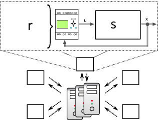
Computational- and network load in event-triggered networked MPC
Measuring transmitted data and computational cost
The remainder of the paper is based on the following assumptions and hypotheses H1-H3: (H1) Bandwidth requirements can be determined by counting the number of bits transferred per event, where real numbers are transmitted using IEEE 754 half precision [1] ( below). (H2) Computational effort can be measured by counting floating point operations, where multiplications and summations cost one floating point operation (flop), and divisions cost ten flops [25]; the cost of some recurring operations is stated in Table 1 [10, chap. 1.1.15] [8, p.12]. (H3) The central node is assumed to carry out all computations instantaneously.
Let the term computational load on the local node refer to the number of flops necessary to determine the control law and polytope (7). Since all variants discussed below have the evaluation of the control law (7a) and condition (8) in common, we neglect the flops required for (7a) and (8).
| op. | ||||
|---|---|---|---|---|
| flops |
For any , , and . Existence of the inverse and are assumed in the last column.
Trade-off between transmitted data and local calculations
A control law and polytope must be sent across the network whenever an event (8) occurs. It is evident from (7) that the matrices and define the control law and polytope. It suffices to send much less data, however. This is stated more precisely in Lemma 2, which was proved in [5].
Lemma 2
Equation (9b) may tempt the reader to think we use the input signals of , which is open-loop but in general not closed-loop optimal. We stress again this is not the case, but we use the feedback law (7a) and polytope (7b), because this feedback law is closed-loop optimal on the polytope. Because we determine a new law and polytope whenever the current polytope is left, the same closed-loop optimal sequence as solving (2) in every time step results. Therefore, the same closed-loop optimal system behavior is obtained as solving (2) or (3) in every time step [16]. The claim about (9b) in Lemma 2 holds, because defines according to (5) and defines , , , and thus the law and polytope according to (6).
Lemma 2 implies the following alternative approaches A1-A4 for transmitting the optimal control law (7a) and its polytope (7b).
- A1
- A3
- A5
- A7
Determine , , , on the central node and send them to the local node.
These four approaches obviously differ with respect to the amount of data sent across the network and the computational effort on the local node. More precisely, we have the following results, which are taken from [5].
Lemma 3
Assume H1-H4 hold. Furthermore, assume (2) or equivalently (3) has been solved for an on the central node. Then the number of bits that need to be transmitted in approaches A1-A4 and the number of flops required on the local node for approaches A1-A4 are as follows:
| bits | flops | |
|---|---|---|
| A1 | ||
| A2 | ||
| A3 | ||
| A4 | ||
Based on the technical results stated in Lemma 3, it is now easy to compare approaches A1-A4. We compare the amount of transmitted data first.
Proposition 4
Proof: Statement (i) is obvious, since A1 requires to transmit and approach A3 requires to transmit and . Statement (ii) can be shown by substituting (box constraints) into the number of transmitted bits stated in Lemma 3 and subtracting the number of bits for A1 - A5 from those for A7 . Since the resulting expressions are always positive, statement (ii) holds. In order to prove (iii) we need to show that (12) implies
| (14) |
For (box constraints), this is equivalent to
| (15) |
It is easy to show implies . Therefore,
| (16) |
implies (15), i.e., (14) for box constraints. Rearranging (16) yields the desired condition (12). Part (iv) can be shown in the same way as (iii).
Since states and inputs are constrained by an upper and lower bound in many technical systems, the introduction of box constraints in part (ii) - (iv) of Proposition 4 is not a severe restriction.
Proposition 4 reveals the following partial order of the approaches with respect to the number of transmitted bits: Approach A1 requires the smallest number of transmitted bits, followed by approaches A3 and A7 . Approach A5 results in less transmitted data than A1 if inequality (12) is not fulfilled and less transmitted data than approach A3 if inequality (13) is not fulfilled. It remains to compare the computational effort on the local node based on Lemma 2.
Proposition 5
Proof: Statement (iii) is obvious from the zero in the last row and column of the table in Lemma 3. Statements (i) and (ii) can be shown by subtracting the number of flops given in the third column of the table in Lemma 3 for the respective pair of approaches. Specifically, this difference reads for approach A1 . Since this expression is positive, approach A1 never requires less operations than approach A3 . Statement (ii) can be shown in the same way.
None of the approaches A1 - A7 results in both, the smallest number of transmitted bits and the smallest computational effort. Since the number of transmitted bits in approach A3 depends on (see (13)), and since approach A5 depends on (12), the best trade-off results for transmitting the active set of constraints in approach A1 . We examine A1 in more detail in the remainder of the paper.
Computational effort of approach A1
While only bits need to be transmitted in approach A1 , additional computations must be carried out on the local node. Most importantly, the inverse of has to be determined on the local node, which requires on the order of operations (see, e.g., [8], p.12). However, the absolute number of operations for this inversion always remains small compared to the number of operations necessary for evaluating (6), even though the latter scales linearly only in . This statement is made more precise in the following proposition for the special case of box constraints. Note that the proposition is conservative in the sense that the computational effort for the inversion is even smaller in practice (see Section 4).
Proposition 6
Proof: The inversion in (6) requires
flops according to [8, p.12]. Subtracting this figure from the overall number of operations for A1 as stated in Lemma 3 yields
which equals the number of flops for all matrix operations but the inversion in A1 . It is easy to show that , , and imply and . We now show that if
| (18) |
holds for a , it holds for all . This can be seen by extending to a real variable and showing is strictly increasing by proving . Applying the quotient rule yields a fraction with numerator
| (19) |
and denominator . Since the denominator is positive, it suffices to show (19) is positive, which can equivalently be stated as
This condition obviously holds for , and . It remains to be shown that (18) is positive for the largest possible number of concurrently active constraints . This number reads for box constraints with . All combinations of , and are covered by the three cases
| (i) | |||
| (ii) | |||
| (iii) |
where (i) and (ii) together cover , , . Case (i), i.e., substituting and into (18) and rearranging yields the condition , which obviously holds for all . Case (ii), i.e., substituting into (18) and rearranging yields the condition
| (20) |
Now implies and for all . Adding these two inequalities to , which also holds for all , shows that condition (20) holds. Case (iii) can be shown by noting that (18) can equivalently be stated as
| (21) | ||||
for arbitrary , and . It is easy to see that and imply the first three terms on the left hand side of (21) are larger than the first term on the right hand side for all . Similarly, the 4th and 5th term on the left hand side of (21) together dominate the second term on the right hand side, and the last term on the left hand side dominates the remaining two terms on the right hand side. Since the remaining terms on the left hand side are positive, condition (21) holds.
Implementation on industrial hardware
We use a SIMATIC IPC847C industrial computer (IPC for short) with an Intel Core i7-610E CPU and 8GB memory11 1 See http://www.siemens.com for more information about the IPC, PLC and I/O modules (checked on October 7, 2016). as the central node. The IPC runs a QNX Neutrino 6.5.0 real-time operating system and is programmed in ISO C++. The local node consists of a Siemens S7-400 PLC equipped with 30MB memory, an SM 331 module, and an SM 332 analog I/O module22footnotemark: 2 . We use statement lists (STL) to program the PLC. The system that is controlled by the PLC is simulated on a dSpace22 2 See https://www.dspace.com for more information (checked on October 7, 2016). HIL system. System states and inputs are exchanged via analog I/Os. We refer to this equipment as HIL setup for brevity.
Computation times are measured on the PLC by setting a digital output to high every time the computational task starts, and to low when it finishes. Closer inspection of these measurements reveals that the digital I/O modules of the PLC have a small random delay. We repeat measurements ten times to reduce the influence of this delay. This results in standard deviations of less than 3% for all reported data.
The communication between the nodes is performed by a PROFIBUS network, but we stress that any other bus system can be used instead. The network is only used when the local node triggers the central node to calculate a new affine control law and polytope.
Implementation details
We use a simple code generator to generate the required STL code from the problem (2) in Matlab. The code generator precomputes matrices offline. The evaluation of (6) exploits common subexpressions. The inversion of is replaced by a LU decomposition with pivoting and forward-backward substitutions. The code generator also generates a C++ header file for the IPC which provides matrices of the QP (3). We use OOQP (see [9]) to solve QPs on the IPC.
Since data transmission and calculations (3), (6) may be necessary to obtain the control input , a delay between measuring the state and applying the control input may occur. However, the delay only occurs if in (8). Consequently, depending on whether or in (8), the computation of the control input differs. We explain these two cases in more detail. Let and refer to the current and subsequent state of the closed-loop system, and let be a polytope with . While is known from a measurement, is predicted at sampling interval with the system model (2b). Either one of the following two cases applies in every time step:
(i) If , the control law and polytope in the subsequent time step remain the same as in time step . The control input is calculated at the beginning of sampling interval on the local node and is applied to the system. In this case no communication with the central node is necessary.
(ii) If , the QP (3) must be solved on the central node and a new control law and polytope must be calculated locally. The time between two consecutive sampling intervals and can be used to compute the control law and polytope (7) that are required in time step : We transfer the predicted state to the central node, solve the quadratic program (3) and transfer data according to approaches A1 - A7 back to the local node. Once the information is available on the local node, matrices of the control law and polytope are calculated. By solving (3) for the predicted state , the control law and polytope are obtained for time step . The control input is calculated at the beginning of the next sampling interval by evaluating the predicted control law.
Validation of the implementation
We validated the implementation on the PLC and the IPC by regulating the simple double integrator from [24] to the origin for 100 random initial states and comparing the state space trajectories that resulted from the HIL setup to reference trajectories simulated in Matlab. A mean squared error resulted, where a total of time steps arose for the 100 random initial conditions. The error results from analog to digital and digital to analog conversion errors, and random noise on the analog signal.
Results
We measure computation times of approach A1 running on the HIL setup described in Section 4. The results corroborate Proposition 6.
Example system
Consider the mechanical system with four oscillating masses connected by springs sketched in Fig. 3. Three inputs () are used to control tension between the masses. Masses and spring constants have the value one and there is no damping. The resulting continuous time system
| (22) | ||||
|
|
|
|||
|
|
|
is discretized with zero order hold and a sampling time of seconds. State variables and input variables are subject to the constraints and . Cost function matrices are chosen to be and , and is set to the solution of the discrete-time algebraic Riccati equation. The horizon of the MPC problem is chosen to be . The number of simultaneously active constraints is bounded above according to
| (23) |
Hardware in the loop test
Approach A1 provides the best trade-off of data transmission to computational cost on the local node. We conduct measurements of the computation times on the local node with the HIL setup described in Section 4 to analyze approach A1 in more detail. Specifically, we report actual computational times of the HIL system for the following tasks to corroborate Proposition 6:
- a)
transferring the current system state to the central node, solving the QP on the central node, and sending as defined in (10) to the local node,
- b)
evaluation of (6) on the local node,
- c)
computing the control input and evaluating condition (7) on the local node.
We assume that flops and computation times are related by a constant factor, i.e.
| (24) |
for some .
The computational times that result for 100 random feasible initial conditions are summarized in Fig. 5. The times required for tasks a, b and c can be approximated by a constant, a cubic function, and a constant, respectively. The time required for task c is obviously small compared to those of tasks a and b, which demonstrates that the control input can be computed with very low computational effort if . The time required for task b dominates the computational time required on the local node for all but very small .
As suggested by Proposition 6, we further analyze the computation time for task b by splitting it into the time necessary to calculate the inverse of and the time required for all remaining matrix operations in (6). Figure 5 shows the two contributions
| (25) |
Substituting
| (26) |
which holds according to Proposition 6 and with (24), results in
| (27) |
This can be understood as an upper bound on , which is also shown in Fig. 5. It is evident from Fig. 5 that the absolute contribution of remains small despite the cubic dependence of on . We conclude approach A1 is the best one of the four variants, because the inversion of required in A1 but not in A3 results in only a small additional computational effort on the local node. Note that this result does not only apply to the example, but the bound (17) established in Proposition 6 applies in general.
Conclusion and outlook
We analyzed the practical usefulness of a networked event-triggered MPC approach by implementing it on industrial hardware. The proposed approach combines a powerful compute node, which solves optimal control problems on demand, with lean local nodes that control local systems with simple affine, regional optimal feedback laws. The local nodes use their feedback laws as long as they are optimal and otherwise request a new law from the central node. Several options for an implementation exist that differ with respect to their balance of local computational effort and network bandwidth requirements. We extended earlier theoretical results to determine the best variant among these choices and corroborated the theoretically expected features of the selected variant with an implementation on industrial control hardware.
An extension to tube-based robust MPC is possible (see [23] for a simulation-based analysis). We believe an extension in this direction is more of theoretical interest, because the case treated in the present paper inherits the robustness of the regional approach [5]. This aspect is currently under investigation.
The proposed approach is based on the idea that once the set of active constraints is known for the current system state, an optimal feedback law and the polytope on which it is optimal are known (see Lemma 2). This also holds in nonlinear MPC with discrete-time system models [20, 6]. It therefore suffices to send the active sets across the network in nonlinear MPC. However, the local nodes must solve nonlinear systems of equations in this case, while affine control laws only need to be evaluated in the linear MPC case. It remains to investigate how the computational effort on the local nodes can be reduced, for example by sending redundant information as in approach A3 .
Finally, future work must combine the proposed approach with methods for predicting the sequence of affine laws along the closed-loop trajectory [4]. This will help reducing the number of optimal control problems further in particular far from the origin, where the affine laws are not reused frequently.
Acknowledgment
Support by the Deutsche Forschungsgemeinschaft (DFG) under the grant MO 1086/15-1 is gratefully acknowledged.
References
- [1] IEEE standard for binary floating-point arithmetic. ANSI/IEEE Std 754-1985.
- [2] A. Bemporad, M. Morari, V. Dua and E. N. Pistikopoulos. The explicit linear quadratic regulator for constrained systems. Automatica, 38(1):3 – 20, 2002.
- [3] D. Bernardini and A. Bemporad. Energy-aware robust model predictive control based on noisy wireless sensors. Automatica, 48(1):36 – 44, 2012.
- [4] P. S. Berner, K. König, M. Kvasnica, and M. Mönnigmann. Active set updates in event-triggered networked MPC. Accepted for European Control Conference (ECC), 2019.
- [5] P. S. Berner and M. Mönnigmann. A comparison of four variants of event-triggered networked MPC. In Proceedings of the 2016 IEEE Multi-Conference on Systems and Control, pages 1519–1524, 2016.
- [6] L. F. Domínguez and E. N. Pistikopoulos. Recent advances in explicit multiparametric nonlinear model predictive control. Industrial & Engineering Chemistry Research, 50(2):609–619, 2011.
- [7] A. Eqtami, D. Dimarogonas, and K. Kyriakopoulos. Event-triggered strategies for decentralized model predictive controllers. In Proceedings of the 18th IFAC World Congress, pages 10068–10073, 2011.
- [8] R. Farebrother. Linear Least Squares Computations. Statistics: A Series of Textbooks and Monographs. Taylor & Francis, 1988.
- [9] E. M. Gertz and S. J. Wright. Object-oriented software for quadratic programming. ACM Transactions on Mathematical Software, 29(1):58–81, 2003.
- [10] G. H. Golub and C. F. Van Loan. Matrix Computations. The Johns Hopkins University Press, fourth edition, 2013.
- [11] W. P. M. H. Heemels, K. H. Johansson, and P. Tabuada. An introduction to event-triggered and self-triggered control. In Proceedings of the 51st IEEE Conference on Decision and Control (CDC), pages 3270–3285, 2012.
- [12] B. Houska, H. J. Ferreau, and M. Diehl. ACADO Toolkit – An Open Source Framework for Automatic Control and Dynamic Optimization. Optimal Control Appl. and Methods, 32(3):298–312, 2011.
- [13] B. Huyck, H. J. Ferreau, M. Diehl, J. De Brabanter, J. F. M. Van Impe, B. De Moor, and F. Logist. Towards online model predictive control on a programmable logic controller: Practical considerations. Mathematical Problems in Engineering, 2012:1–20, 2012.
- [14] G. P. Incremona, A. Ferrara, and L. Magni. Asynchronous networked MPC with ISM for uncertain nonlinear systems. IEEE Transactions on Automatic Control, 62(9):4305–4317, Sept 2017.
- [15] M. Jost, G. Pannocchia, and M. Mönnigmann. Online constraint removal: Accelerating MPC with a Lyapunov function. Automatica, 57:164 – 169, 2015.
- [16] M. Jost, M. Schulze Darup, and M. Mönnigmann. Optimal and suboptimal event-triggering in linear model predictive control. In Proceedings of the 2015 European Control Conference (ECC), pages 1147–1152, 2015.
- [17] D. K. M. Kufoalor, S. Richter, L. Imsland, T. A. Johansen, M. Morari, and G. O. Eikrem. Embedded model predictive control on a PLC using a primal-dual first-order method for a subsea separation process. In Proceedings of the 22nd Mediterranean Conference on Control and Automation (MED), pages 368–373, 2014.
- [18] J. Maciejowski. Predictive Control: With Constraints. Pearson Education. Prentice Hall, 2002.
- [19] J. Mattingley, Y. Wang, and S. Boyd. Code generation for receding horizon control. In Proceedings of the International Symposium on Computer-Aided Control System Design (CACSD), pages 985–992, 2010.
- [20] M. Mönnigmann, J. Otten, and M. Jost. Nonlinear MPC defines implicit regional optimal control laws. IFAC-PapersOnLine, 48(23):142 – 147, 2015. 5th IFAC Conference on Nonlinear Model Predictive Control NMPC 2015.
- [21] G. Pannocchia, J. B. Rawlings, and S. J. Wright. Fast, large-scale model predictive control by partial enumeration. Automatica, 43(5):852–860, 2007.
- [22] I. Rauová, R. Valo, M. Kvasnica, and M. Fikar. Real-time model predictive control of a fan heater via PLC. In Proceedings of the 18th International Conference on Process Control, pages 388–393, 2011.
- [23] M. Schulze Darup, R. Dyrska, K. König, and M. Mönnigmann. A novel event-triggered robust MPC scheme for linear systems. In Proceedings of the 56th IEEE Conference on Decision and Control (CDC), pages 2941–2946, 2017.
- [24] M. Seron, G. Goodwin, and J. D. Doná. Characterisation of receding horizon control for constrained linear systems. Asian Journal of Control, 5(2):271 – 286, 2003.
- [25] C. Ueberhuber. Numerical Computation 1: Methods, Software, and Analysis. Numerical Computation 1 Vol. XVI. Springer Berlin Heidelberg, 1997.
- [26] G. Valencia-Palomo and J. Rossiter. Efficient suboptimal parametric solutions to predictive control for PLC applications. Control Engineering Practice, 19(7):732 – 743, 2011.
- [27] P. Varutti, B. Kern, T. Faulwasser, and R. Findeisen. Event-based model predictive control for networked control systems. In Proceedings of the 48th IEEE Conference on Decision and Control, jointly with the 28th Chinese Control Conference (CDC/CCC), pages 567–572, 2009.
- [28] P. Zometa, M. Kögel, and R. Findeisen. AO-MPC: a free code generation tool for embedded real-time linear model predictive control. In Proceedings of the American Control Conf., pages 5320–5325, 2013.