Monte Carlo Co-Ordinate Ascent Variational Inference

Lifeng Ye Affiliation: Department of Statistical Science, University College London Alexandros Beskos Affiliation: Department of Statistical Science, University College London Maria De Iorio Affiliation: Department of Statistical Science, University College London Affiliation: Yale-NUS College, Singapore Jie Hao Affiliation: lifeng.ye.13@ucl.ac.uk, a.beskos@ucl.ac.uk, maria@yale-nus.edu.sg, j.hao@sjtu.edu.cn Affiliation: Key Laboratory of Systems Biomedicine (Ministry of Education), Shanghai Center for Systems Biomedicine, Shanghai Jiao Tong University

Abstract

In Variational Inference (VI), coordinate-ascent and gradient-based approaches are two major types of algorithms for approximating difficult-to-compute probability densities. In real-world implementations of complex models, Monte Carlo methods are widely used to estimate expectations in coordinate-ascent approaches and gradients in derivative-driven ones. We discuss a Monte Carlo Co-ordinate Ascent VI (MC-CAVI) algorithm that makes use of Markov chain Monte Carlo (MCMC) methods in the calculation of expectations required within Co-ordinate Ascent VI (CAVI). We show that, under regularity conditions, an MC-CAVI recursion will get arbitrarily close to a maximiser of the evidence lower bound (ELBO) with any given high probability. In numerical examples, the performance of MC-CAVI algorithm is compared with that of MCMC and – as a representative of derivative-based VI methods – of Black Box VI (BBVI). We discuss and demonstrate MC-CAVI’s suitability for models with hard constraints in simulated and real examples. We compare MC-CAVI’s performance with that of MCMC in an important complex model used in Nuclear Magnetic Resonance (NMR) spectroscopy data analysis – BBVI is nearly impossible to be employed in this setting due to the hard constraints involved in the model.

Keyword: Variational Inference; Markov chain Monte Carlo; Coordinate-Ascent;
Gradient-Based Optimisation; Bayesian Inference; Nuclear Magnetic Resonance.

1 Introduction

Variational Inference (VI) (Jordan et al. 1999; Wainwright et al. 2008) is a powerful method to approximate intractable integrals. As an alternative strategy to Markov chain Monte Carlo (MCMC) sampling, VI is fast, relatively straightforward for monitoring convergence and typically easier to scale to large data (Blei et al. 2017) than MCMC. The key idea of VI is to approximate difficult-to-compute conditional densities of latent variables, given observations, via use of optimization. A family of distributions is assumed for the latent variables, as an approximation to the exact conditional distribution. VI aims at finding the member, amongst the selected family, that minimizes the Kullback-Leibler (KL) divergence from the conditional law of interest.

Let $x$ and $z$ denote, respectively, the observed data and latent variables. The goal of the inference problem is to identify the conditional density (assuming a relevant reference measure, e.g. Lebesgue) of latent variables given observations, i.e. $p(z|x)$ . Let $\mathcal{L}$ denote a family of densities defined over the space of latent variables – we denote members of this family as $q=q(z)$ below. The goal of VI is to find the element of the family closest in KL divergence to the true $p(z|x)$ . Thus, the original inference problem can be rewritten as an optimization one: identify $q^{*}$ such that

q^{*}=\operatornamewithlimits{argmin}\limits_{q\in\mathcal{L}}\textrm{KL}(q\mid p(\cdot|x))

(1)

for the KL-divergence defined as

	$\displaystyle\textrm{KL}(q\mid p(\cdot\|x))$	$\displaystyle=\mathbb{E}_{q}[\log q(z)]-\mathbb{E}_{q}[\log p(z\|x)]$
		$\displaystyle=\mathbb{E}_{q}[\log q(z)]-\mathbb{E}_{q}[\log p(z,x)]+\log p(x),$

with $\log p(x)$ being constant w.r.t. $z$ . Notation $\mathbb{E}_{q}$ refers to expectation taken over $z\sim q$ . Thus, minimizing the KL divergence is equivalent to maximising the evidence lower bound, ELBO $(q)$ , given by

\textrm{ELBO}(q)=\mathbb{E}_{q}[\log p(z,x)]-\mathbb{E}_{q}[\log q(z)].

(2)

Let $\mathsf{S}_{p}\subseteq\mathbb{R}^{m}$ , $m\geq 1$ , denote the support of the target $p(z|x)$ , and $\mathsf{S}_{q}\subseteq\mathbb{R}^{m}$ the support of a variational density $q\in\mathcal{L}$ – assumed to be common over all members $q\in\mathcal{L}$ . Necessarily, $\mathsf{S}_{p}\subseteq\mathsf{S}_{q}$ , otherwise the KL-divergence will diverge to $+\infty$ .

Many VI algorithms focus on the mean-field variational family, where variational densities in $\mathcal{L}$ are assumed to factorise over blocks of $z$ . That is,

q(z)=\prod_{i=1}^{b}q_{i}(z_{i}),\quad\mathsf{S}_{q}=\mathsf{S}_{q_{1}}\times\cdots\times\mathsf{S}_{q_{b}},\quad z=(z_{1},\ldots,z_{b})\in\mathsf{S}_{q},\,\,\,z_{i}\in\mathsf{S}_{q_{i}},

(3)

for individual supports $\mathsf{S}_{q_{i}}\subseteq\mathbb{R}^{m_{i}}$ , $m_{i}\geq 1$ , $1\leq i\leq b$ , for some $b\geq 1$ , and $\sum_{i}m_{i}=m$ . It is advisable that highly correlated latent variables are placed in the same block to improve the performance of the VI method.

There are, in general, two types of approaches to maximise ELBO in VI: a co-ordinate ascent approach and a gradient-based one. Co-ordinate ascent VI (CAVI) (Bishop 2006) is amongst the most commonly used algorithms in this context. To obtain a local maximiser for ELBO, CAVI sequentially optimizes each factor of the mean-field variational density, while holding the others fixed. Analytical calculations on function space – involving variational derivatives – imply that, for given fixed $q_{1},\ldots,q_{i-1},q_{i+1},\ldots,q_{b}$ , ELBO $(q)$ is maximised for

q_{i}(z_{i})\propto\exp\big\{\mathbb{E}_{-i}[\log p(z_{i_{-}},z_{i},z_{i_{+}},x)]\big\},

(4)

where $z_{-i}:=(z_{i_{-}},z_{i_{+}})$ denotes vector $z$ having removed component $z_{i}$ , with ${i_{-}}$ (resp. ${i_{+}}$ ) denoting the ordered indices that are smaller (resp. larger) than $i$ ; $\mathbb{E}_{-i}$ is the expectation taken under $z_{-i}$ following its variational distribution, denoted $q_{-i}$ . The above suggest immediately an iterative algorithm, guaranteed to provide values for ELBO $(q)$ that cannot decrease as the updates are carried out.

The expected value $\mathbb{E}_{-i}[\log p(z_{i_{-}},z_{i},z_{i_{+}},x)]$ can be difficult to derive analytically. Also, CAVI typically requires traversing the entire dataset at each iteration, which can be overly computationally expensive for large datasets. Gradient-based approaches, which can potentially scale up to large data – alluding here to recent Stochastic-Gradient-type methods – can be an effective alternative for ELBO optimisation. However, such algorithms have their own challenges, e.g. in the case reparameterization Variational Bayes (VB) analytical derivation of gradients of the log-likelihood can often be problematic, while in the case of score-function VB the requirement of the gradient of $\log q$ restricts the range of the family $\mathcal{L}$ we can choose from.

In real-world applications, hybrid methods combining Monte Carlo with recursive algorithms are common, e.g., Auto-Encoding Variational Bayes, Doubly-Stochastic Variational Bayes for non-conjugate inference, Stochastic Expectation-Maximation (EM) (Beaumont et al. 2002; Sisson et al. 2007; Wei and Tanner 1990). In VI, Monte Carlo is often used to estimate the expectation within CAVI or the gradient within derivative-driven methods. This is the case, e.g., for Stochastic VI (Hoffman et al. 2013) and Black-Box VI (BBVI) (Ranganath et al. 2014).

BBVI is used in this work as a representative of gradient-based VI algorithms. It allows carrying out VI over a wide range of complex models. The variational density $q$ is typically chosen within a parametric family, so finding $q^{*}$ in (1) is equivalent to determining an optimal set of parameters that characterize $q_{i}=q_{i}(\cdot|\lambda_{i})$ , $\lambda_{i}\in\Lambda_{i}\subseteq\mathbb{R}^{d_{i}}$ , $1\leq d_{i}$ , $1\leq i\leq b$ , with $\sum_{i=1}^{b}d_{i}=d$ . The gradient of ELBO w.r.t. the variational parameters $\lambda=(\lambda_{1},\ldots,\lambda_{b})$ equals

\nabla_{\lambda}\textrm{ELBO}(q):=\mathbb{E}_{q}\big[\nabla_{\lambda}\log q(z|\lambda)\{\log p(z,x)-\log q(z|\lambda)\}\big]

(5)

and can be approximated by black-box Monte Carlo estimators as, e.g.,

\widehat{\nabla_{\lambda}\textrm{ELBO}(q)}:=\tfrac{1}{N}\sum^{N}_{n=1}\big[\nabla_{\lambda}\log q(z^{(n)}|\lambda)\{\log p(z^{(n)},x)-\log q(z^{(n)}|\lambda)\}\big],

(6)

with $z^{(n)}\stackrel{{\scriptstyle iid}}{{\sim}}q(z|\lambda)$ , $1\leq n\leq N$ , $N\geq 1$ . The approximated gradient of ELBO can then be used within a stochastic optimization procedure to update $\lambda$ at the $k$ th iteration with

\lambda_{k+1}\leftarrow\lambda_{k}+\rho_{k}\widehat{\nabla_{\lambda_{k}}\textrm{ELBO}(q)},

(7)

where $\{\rho_{k}\}_{k\geq 0}$ is a Robbins-Monro-type step-size sequence (Robbins and Monro 1951). As we will see in later sections, BBVI is accompanied by generic variance reduction methods, as the variability of (6) for complex models can be large.

Remark 1 (Hard Constraints).

Though gradient-based VI methods are some times more straightforward to apply than co-ordinate ascent ones, – e.g. combined with the use of modern approaches for automatic differentiation (Kucukelbir et al. 2017) – co-ordinate ascent methods can still be important for models with hard constraints, where gradient-based algorithms are laborious to apply. (We adopt the viewpoint here that one chooses variational densities that respect the constaints of the target, for improved accuracy.) Indeed, notice in the brief description we have given above for CAVI and BBVI, the two methodologies are structurally different, as CAVI does not necessarily require to be build up via the introduction of an exogenous variational parameter $\lambda$ . Thus, in the context of a support for the target $p(z|x)$ that involves complex constraints, a CAVI approach overcomes this issue naturally by blocking together the $z_{i}$ ’s responsible for the constraints. In contrast, introduction of the variational parameter $\lambda$ creates sometimes severe complications in the development of the derivative-driven algorithm, as normalising constants that depend on $\lambda$ are extremely difficult to calculate analytically and obtain their derivatives. Thus, a main argument spanning this work – and illustrated within it – is that co-ordinate-ascent-based VI methods have a critical role to play amongst VI approaches for important classes of statistical models.

The main contributions of the paper are:

(i)

We discuss, and then apply a Monte Carlo CAVI (MC-CAVI) algorithm in a sequence of problems of increasing complexity, and study its performance. As the name suggests, MC-CAVI uses the Monte Carlo principle for the approximation of the difficult-to-compute conditional expectations, $\mathbb{E}_{-i}[\log p(z_{i_{-}},z_{i},z_{i_{+}},x)]$ , within CAVI.
(ii)

We provide a justification for the algorithm by showing analytically that, under suitable regularity conditions, MC-CAVI will get arbitrarily close to a maximiser of the ELBO with high probability.
(iii)

We contrast MC-CAVI with MCMC and BBVI through simulated and real examples, some of which involve hard constraints; we demonstrate MC-CAVI’s effectiveness in an important application imposing such hard constraints, with real data in the context of Nuclear Magnetic Resonance (NMR) spectroscopy.

Remark 2.

Inserting Monte Carlo steps within a VI approach (that might use a mean field or another approximation) is not uncommon in the VI literature. E.g., Forbes and Fort 2007 employ an MCMC procedure in the context of a Variational EM (VEM), to obtain estimates of the normalizing constant for Markov Random Fields – they provide asymptotic results for the correctness of the complete algorithm; Tran et al. 2016 apply Mean-Field Variational Bayes (VB) for Generalised Linear Mixed Models, and use Monte Carlo for the approximation of analytically intractable required expectations under the variational densities; several references for related works are given in the above papers. Our work focuses on MC-CAVI, and develops theory that is appropriate for this VI method. This algorithm has not been studied analytically in the literature, thus the development of its theoretical justification – even if it borrows elements from Monte Carlo EM – is new.

The rest of the paper is organised as follows. Section 2 presents briefly the MC-CAVI algorithm. It also provides – in a specified setting – an analytical result illustrating non-accumulation of Monte Carlo errors in the execution of the recursions of the algorithm. That is, with a probability arbitrarily close to 1, the variational solution provided by MC-CAVI can be as close as required to the one of CAVI, for a big enough Monte Carlo sample size, regardless of the number of algorithmic iterations. Section 3 shows two numerical examples, contrasting MC-CAVI with alternative algorithms. Section 4 presents an implementation of MC-CAVI in a real, complex, challenging posterior distribution arising in metabolomics. This is a practical application, involving hard constraints, chosen to illustrate the potential of MC-CAVI in this context. We finish with some conclusions in Section 5.

2 MC-CAVI Algorithm

2.1 Description of the Algorithm

We begin with a description of the basic CAVI algorithm. A double subscript will be used to identify block variational densities: $q_{i,k}(z_{i})$ (resp. $q_{-i,k}(z_{-i})$ ) will refer to the density of the $i$ th block (resp. all blocks but the $i$ th), after $k$ updates have been carried out on that block density (resp. $k$ updates have been carried out on the blocks preceding the $i$ th, and $k-1$ updates on the blocks following the $i$ th).

•

Step 0: Initialize probability density functions $q_{i,0}(z_{i})$ , $i=1,\ldots,b$ .
•
Step $k$ : For $k\geq 1$ , given $q_{i,k-1}(z_{i})$ , $i=1,\ldots,b$ , execute:
- –
  
  For $i=1,\ldots,b$ , update:
  
  $\displaystyle\log q_{i,k}(z_{i})=const.+\mathbb{E}_{-i,k}[\log p(z,x)],$
  
  with $\mathbb{E}_{-i,k}$ taken w.r.t. $z_{-i}\sim q_{-i,k}$ .
•

Iterate until convergence.

Assume that the expectations $\mathbb{E}_{-i}[\log p(z,x)]$ , $\{i:i\in\mathcal{I}\}$ , for an index set $\mathcal{I}\subseteq\{1,\ldots,b\}$ , can be obtained analytically, over all updates of the variational density $q(z)$ ; and that this is not the case for $i\notin\mathcal{I}$ . Intractable integrals can be approximated via a Monte Carlo method. (As we will see in the applications in the sequel, such a Monte Carlo device typically uses samples from an appropriate MCMC algorithm.) In particular, for $i\notin\mathcal{I}$ , one obtains $N\geq 1$ samples from the current $q_{-i}(z_{-i})$ and uses the standard Monte Carlo estimate

\widehat{\mathbb{E}}_{-i}[\log p(z_{i_{-}},z_{i},z_{i_{+}},x)]=\frac{\sum_{n=1}^{N}\log p(z_{i_{-}}^{(n)},z_{i},z_{i_{+}}^{(n)},x)}{N}.

Implementation of such an approach gives rise to MC-CAVI, described in Algorithm 1.

Require : Number of iterations

T

Require : Number of Monte Carlo samples

N

Require :

\mathbb{E}_{-i}[\log p(z_{i_{-}},z_{i},z_{i_{+}},x)]

in closed form, for

i\in\mathcal{I}

Initialize

q_{i,0}(z_{i})

i=1,\ldots,b

.
for $k=1:T$ do 1

for $i=1:b$ do 2

i\in\mathcal{I}

, set

q_{i,k}(z_{i})\propto\exp\big\{\mathbb{E}_{-i,k}[\log p(z{{}_{i_{-}}},z_{i},z{{}_{i_{+}}},x)]\big\}

; 3

i\notin\mathcal{I}

:
Obtain

N

samples,

(z_{i_{-},k}^{(n)},z_{i_{+},k-1}^{(n)})

1\leq n\leq N

, from

q_{-i,k}(z_{-i})

.
Set

q_{i,k}(z_{i})\propto\exp\big\{\tfrac{\sum_{n=1}^{N}\textrm{log}\;p(z_{i_{-},k}^{(n)},z_{i},z_{i_{+},k-1}^{(n)},x)}{N}\big\}.

end for 4

end for 5

Algorithm 1 MC-CAVI

2.2 Applicability of MC-CAVI

We discuss here the class of problems for which MC-CAVI can be applied. It is desirable to avoid settings where the order of samples or statistics to be stored in memory increases with the iterations of the algorithm. To set-up the ideas we begin with CAVI itself. Motivated by the standard exponential class of distributions, we work as follows.

Consider the case when the target density $p(z,x)\equiv f(z)$ – we omit reference to the data $x$ in what follows, as $x$ is fixed and irrelevant for our purposes (notice that $f$ is not required to integrate to $1$ ) – is assumed to have the structure,

\displaystyle f(z)=h(z)\exp\big\{\langle\eta,T(z)\rangle-A(\eta)\big\},\quad z\in\mathsf{S}_{p},

(8)

for $s$ -dimensional constant vector $\eta=(\eta_{1},\ldots,\eta_{s})$ , vector function $T(z)=(T_{1}(z),\ldots,T_{s}(z))$ , with some $s\geq 1$ , and relevant scalar functions $h>0$ , $A$ ; $\langle\cdot,\cdot\rangle$ is the standard inner product in $\mathbb{R}^{s}$ . Also, we are given the choice of block-variational densities $q_{1}(z_{1}),\ldots,q_{b}(z_{b})$ in (3). Following the definition of CAVI from Section 2.1 – assuming that the algorithm can be applied, i.e. all required expectations can be obtained analytically – the number of ‘sufficient’ statistics, say $T_{i,k}$ giving rise to the definition of $q_{i,k}$ will always be upper bounded by $s$ . Thus, in our working scenario, CAVI will be applicable with a computational cost that is upper bounded by a constant within the class of target distributions in (8) – assuming relevant costs for calculating expectations remain bounded over the algorithmic iterations.

Moving on to MC-CAVI, following the definition of index set $\mathcal{I}$ in Section 2.1, recall that a Monte Carlo approach is required when updating $q_{i}(z_{i})$ for $i\notin\mathcal{I}$ , $1\leq i\leq b$ . In such a scenario, controlling computational costs amounts to having a target (8) admitting the factorisations,

h(z)\equiv h_{i}(z_{i})h_{-i}(z_{-i}),\quad T_{l}(z)\equiv T_{l,i}(z_{i})T_{l,-i}(z_{-i}),\,\,\,1\leq l\leq s,\quad\,\,\textrm{for all }\,i\notin\mathcal{I}.

(9)

Once (9) is satisfied, we do not need to store all $N$ samples from $q_{-i}(z_{-i})$ , but simply some relevant averages keeping the cost per iteration for the algorithm bounded. We stress that the combination of characterisations in (8)-(9) is very general and will typically be satisfied for most practical statistical models.

2.3 Theoretical Justification of MC-CAVI

An advantageous feature of MC-CAVI versus derivative-driven VI methods is its structural similarity with Monte Carlo Expectation-Maximization (MCEM). Thus, one can build on results in the MCEM literature to prove asymptotical properties of MC-CAVI; see e.g. Chan and Ledolter 1995; Booth and Hobert 1999; Levine and Casella 2001; Fort et al. 2003. To avoid technicalities related with working on general spaces of probability density functions, we begin by assuming a parameterised setting for the variational densities – as in the BBVI case – with the family of variational densities being closed under CAVI or (more generally) MC-CAVI updates.

Assumption 1 (Closedness of Parameterised $q(\cdot)$ Under Variational Update).

For the CAVI or the MC-CAVI algorithm, each $q_{i,k}(z_{i})$ density obtained during the iterations of the algorithm, $1\leq i\leq b$ , $k\geq 0$ , is of the parametric form

q_{i,k}(z_{i})=q_{i}(z_{i}|\lambda_{i}^{k}),

for a unique $\lambda_{i}^{k}\in\Lambda_{i}\subseteq\mathbb{R}^{d_{i}}$ , for some $d_{i}\geq 1$ , for all $1\leq i\leq b$ .
(Let $d=\sum_{i=1}^{b}{d_{i}}$ and $\Lambda=\Lambda_{1}\times\cdots\times\Lambda_{b}$ .)

Under Assumption 1, CAVI and MC-CAVI can be corresponded to some well-defined maps $M:\Lambda\mapsto\Lambda$ , $\mathcal{M}_{N}:\Lambda\mapsto\Lambda$ respectively, so that, given current variational parameter $\lambda$ , one step of the algorithms can be expressed in terms of a new parameter $\lambda^{\prime}$ (different for each case) obtained via the updates

\textrm{CAVI:}\,\,\,\,\lambda^{\prime}=M(\lambda);\qquad\textrm{MC-CAVI:}\,\,\,\,\lambda^{\prime}=\mathcal{M}_{N}(\lambda).

For an analytical study of the convergence properties of CAVI itself and relevant regularity conditions, see e.g. (Bertsekas 1999, Proposition 2.7.1), or numerous other resources in numerical optimisation. Expressing the MC-CAVI update – say, the $(k+1)$ th one – as

\lambda^{k+1}=M(\lambda^{k})+\{\mathcal{M}_{N}(\lambda^{k})-M(\lambda^{k})\},

(10)

it can be seen as a random perturbation of a CAVI step. In the rest of this section we will explore the asymptotic properties of MC-CAVI. We follow closely the approach in Chan and Ledolter 1995 – as it provides a less technical procedure, compared e.g. to Fort et al. 2003 or other works about MCEM – making all appropriate adjustments to fit the derivations into the setting of the MC-CAVI methodology along the way. We denote by $M^{k}$ , $\mathcal{M}_{N}^{k}$ , the $k$ -fold composition of $M$ , $\mathcal{M}_{N}$ respectively, for $k\geq 0$ .

Assumption 2.

$\Lambda$ is an open subset of $\mathbb{R}^{d}$ , and the mappings $\lambda\mapsto\textrm{ELBO}(q(\lambda))$ , $\lambda\mapsto M(\lambda)$ are continuous on $\Lambda$ .

If $M(\lambda)=\lambda$ for some $\lambda\in\Lambda$ , then $\lambda$ is a fixed point of $M()$ . A given $\lambda^{*}\in\Lambda$ is called an isolated local maximiser of the ELBO $(q(\cdot))$ if there is a neighborhood of $\lambda^{*}$ over which $\lambda^{*}$ is the unique maximiser of the ELBO $(q(\cdot))$ .

Assumption 3 (Properties of $M(\cdot)$ Near a Local Maximum).

Let $\lambda^{*}\in\Lambda$ be an isolated local maximum of ELBO $(q(\cdot))$ . Then,

(i)

$\lambda^{*}$ is a fixed point of $M(\cdot)$ ;
(ii)

there is a neighborhood $V\subseteq\Lambda$ of $\lambda^{*}$ over which $\lambda^{*}$ is a unique maximum, such that $\textrm{ELBO}(q(M(\lambda)))>\textrm{ELBO}(q(\lambda))$ for any $\lambda\in V\backslash\{\lambda^{*}\}$ .

Notice that the above assumption refers to the deterministic update $M(\cdot)$ , which performs co-ordinate ascent; thus requirements (i), (ii) are fairly weak for such a recursion. The critical technical assumption required for delivering the convergence results in the rest of this section is the following one.

Assumption 4 (Uniform Convergence in Probability on Compact Sets).

For any compact set $C\subseteq\Lambda$ the following holds: for any $\varrho,\varrho^{\prime}>0$ , there exists a positive integer $N_{0}$ , such that for all $N\geq N_{0}$ we have,

\inf_{\lambda\in C}\mathrm{Prob}\,\big[\,\big|\mathcal{M}_{N}(\lambda)-M(\lambda)\big|<\varrho\,\big]>1-\varrho^{\prime}.

It is beyond the context of this paper to examine Assumption 4 in more depth. We will only stress that Assumption 4 is the sufficient structural condition that allows to extend closeness between CAVI and MC-CAVI updates in a single algorithmic step into one for arbitrary number of steps.

We continue with a definition.

Definition 1.

A fixed point $\lambda^{*}$ of $M(\cdot)$ is said to be asymptotically stable if,

(i)

for any neighborhood $V_{1}$ of $\lambda^{*}$ , there is a neighborhood $V_{2}$ of $\lambda^{*}$ such that for all $k\geq 0$ and all $\lambda\in V_{2}$ , $M^{k}(\lambda)\in V_{1}$ ;
(ii)

there exists a neighbourhood $V$ of $\lambda^{*}$ such that $\lim_{k\rightarrow\infty}M^{k}(\lambda)=\lambda^{*}$ if $\lambda\in V$ .

We will state the main asymptotic result for MC-CAVI in Theorem 1 that follows; first we require Lemma 1.

Lemma 1.

Let Assumptions 1-3 hold. If $\lambda^{*}$ is an isolated local maximiser of $\textrm{ELBO}(q(\cdot))$ , then $\lambda^{*}$ is an asymptotically stable fixed point of $M(\cdot)$ .

The main result of this section is as follows.

Theorem 1.

Let Assumptions 1-4 hold and $\lambda^{*}$ be an isolated local maximiser of $\mathrm{ELBO}(q(\cdot))$ . Then there exists a neighbourhood, say $V_{1}$ , of $\lambda^{*}$ such that for starting values $\lambda\in V_{1}$ of MC-CAVI algorithm and for all $\epsilon_{1}>0$ , there exists a $k_{0}$ such that

\lim_{N\rightarrow\infty}\mathrm{Prob}\,\big(\,|\mathcal{M}_{N}^{k}-\lambda^{*}|<\epsilon_{1}\textrm{ for some }k\leq k_{0}\,\big)=1.

The proofs of Lemma 1 and Theorem 1 can be found in Appendices A and B, respectively.

2.4 Stopping Criterion and Sample Size

The method requires the specification of the Monte Carlo size $N$ and a stopping rule.

Principled - but Impractical - Approach

As the algorithm approaches a local maximum, changes in ELBO should be getting closer to zero. To evaluate the performance of MC-CAVI, one could, in principle, attempt to monitor the evolution of ELBO during the algorithmic iterations. For current variational distribution $q=(q_{1},\ldots,q_{b})$ , assume that MC-CAVI is about to update $q_{i}$ with $q^{\prime}_{i}=q^{\prime}_{i,N}$ , where the addition of the second subscript at this point emphasizes the dependence of the new value for $q_{i}$ on the Monte Carlo size $N$ . Define,

\Delta\mathrm{ELBO}(q,N)=\mathrm{ELBO}(q_{i-},q^{\prime}_{i,N},q_{i+})-\mathrm{ELBO}(q).

If the algorithm is close to a local maximum, $\Delta$ ELBO $(q,N)$ should be close to zero, at least for sufficiently large $N$ . Given such a choice of $N$ , an MC-CAVI recursion should be terminated once $\Delta$ ELBO $(q,N)$ is smaller than a user-specified tolerance threshold. Assume that the random variable $\Delta$ ELBO $(q,N)$ has mean $\mu=\mu(q,N)$ and variance $\sigma^{2}=\sigma^{2}(q,N)$ . Chebychev’s inequality implies that, with probability greater than or equal to $(1-1/K^{2})$ , $\Delta$ ELBO $(q,N)$ lies within the interval $(\mu-K\sigma,\mu+K\sigma)$ , for any real $K>0$ . Assume that one fixes a large enough $K$ . The choice of $N$ and of a stopping criterion should be based on the requirements:

(i)

$\sigma\leq\nu$ , with $\nu$ a predetermined level of tolerance;
(ii)

the effective range $(\mu-K\sigma,\mu+K\sigma)$ should include zero, implying that $\Delta$ ELBO $(q,N)$ differs from zero by less than $2K\sigma$ .

Requirement (i) provides a rule for the choice of $N$ – assuming applied over all $1\leq i\leq b$ , for $q$ in areas close to a maximiser –, and requirement (ii) a rule for defining a stopping criterion. Unfortunately, the above considerations – based on the proper term ELBO $(q)$ that VI aims to maximise – involve quantities that are typically impossible to obtain analytically or via some reasonably expensive approximation.

Practical Considerations

Similarly to MCEM, it is recommended that $N$ gets increased as the algorithm becomes more stable. It is computationally inefficient to start with a large value of $N$ when the current variational distribution can be far from the maximiser. In practice, one may monitor the convergence of the algorithm by plotting relevant statistics of the variational distribution versus the number of iterations. We can declare that convergence has been reached when such traceplots show relatively small random fluctuations (due to the Monte Carlo variability) around a fixed value. At this point, one may terminate the algorithm or continue with a larger value of $N$ , which will further decrease the traceplot variability. In the applications we encounter in the sequel, we typically have $N\leq 100$ , so calculating, for instance, Effective Sample Sizes to monitor the mixing performance of the MCMC steps is not practical.

3 Numerical Examples – Simulation Study

In this section we illustrate MC-CAVI with two simulated examples. First, we apply MC-CAVI and CAVI on a simple model to highlight main features and implementation strategies. Then, we contrast MC-CAVI, MCMC, BBVI in a complex scenario with hard constraints.

3.1 Simulated Example 1

We generate $n=10^{3}$ data points from $\mathrm{N}(10,100)$ and fit the semi-conjugate Bayesian model

	Example Model 1
	$\displaystyle{x_{1},\ldots,x_{n}}$	$\displaystyle\sim\mathrm{N}(\vartheta,\tau^{-1}),$
	$\displaystyle\vartheta$	$\displaystyle\sim\mathrm{N}(0,\tau^{-1}),$
	$\displaystyle\tau$	$\displaystyle\sim\textrm{Gamma}(1,1).$

Let $\bar{x}$ be the data sample mean. In each iteration, the CAVI density function – see (4) – for $\tau$ is that of the Gamma distribution $\textrm{Gamma}(\tfrac{n+3}{2},\zeta)$ , with

\displaystyle\zeta=1+\tfrac{(1+n)\mathbb{E}(\vartheta^{2})-2(n\bar{x})\mathbb{E}(\vartheta)+\sum^{n}_{j=1}x^{2}_{j}}{2},

whereas for $\vartheta$ that of the normal distribution $\mathrm{N}(\frac{n\bar{x}}{1+n},\frac{1}{(1+n)\mathbb{E}(\tau)})$ . $(\mathbb{E}(\vartheta),\mathbb{E}(\vartheta^{2}))$ and $\mathbb{E}(\tau)$ denote the relevant expectations under the current CAVI distributions for $\vartheta$ and $\tau$ respectively; the former are initialized at 0 – there is no need to initialise $\mathbb{E}(\tau)$ in this case. Convergence of CAVI can be monitored, e.g., via the sequence of values of $\theta:=(1+n)\mathbb{E}(\tau)$ and $\zeta$ . If the change in values of these two parameters is smaller than, say, $0.01\%$ , we declare convergence. Figure 1 shows the traceplots of $\theta$ , $\zeta$ .

Refer to caption — Figure 1: Tracplots of $\zeta$ (left), $\theta$ (right) from application of CAVI on Simulated Example 1.

Convergence is reached within 0.0017secs¹¹ 1 A Dell Latitude E5470 with Intel(R) Core(TM) i5-6300U CPU@2.40GHz is used for all experiments in this paper., after precisely two iterations, due to the simplicity of the model. The resulted CAVI distribution for $\vartheta$ is $\mathrm{N}(9.6,0.1)$ , and for $\tau$ it is Gamma $(501.5,50130.3)$ so that $\mathbb{E}(\tau)\approx 0.01$ .

Assume now that $q(\tau)$ was intractable. Since $\mathbb{E}(\tau)$ is required to update the approximate distribution of $\vartheta$ , an MCMC step can be employed to sample $\tau_{1},\ldots,\tau_{N}$ from $q(\tau)$ to produce the Monte Carlo estimator $\widehat{\mathbb{E}}(\tau)=\sum^{N}_{j=1}\tau_{j}/N$ . Within this MC-CAVI setting, $\widehat{\mathbb{E}}(\tau)$ will replace the exact ${\mathbb{E}}(\tau)$ during the algorithmic iterations. $(\mathbb{E}(\vartheta),\mathbb{E}(\vartheta^{2}))$ are initialised as in CAVI. For the first 10 iterations we set $N=10$ , and for the remaining ones, $N=10^{3}$ to reduce variability. We monitor the values of $\widehat{\mathbb{E}}(\tau)$ shown in Figure 2.

The figure shows that MC-CAVI has stabilized after about $15$ iterations; algorithmic time was 0.0114secs. To remove some Monte Carlo variability, the final estimator of $\mathbb{E}(\tau)$ is produced by averaging the last 10 values of its traceplot, which gives $\widehat{\mathbb{E}}(\tau)=0.01$ , i.e. a value very close to the one obtained by CAVI. The estimated distribution of $\vartheta$ is $\mathrm{N}(9.6,0.1)$ , the same as with CAVI.

The performance of MC-CAVI depends critically on the choice $N$ . Let A be the value of $N$ in the burn-in period, B the number of burn-in iterations and C the value of $N$ after burn-in. Figure 3 shows trace plots of $\widehat{\mathbb{E}}(\tau)$ under different settings of the triplet A-B-C.

A-B-C	$10$ - $10$ - $10^{5}$	$10^{3}$ - $10$ - $10^{5}$	$10^{5}$ - $10$ - $10^{5}$	$10$ - $30$ - $10^{5}$	$10$ - $50$ - $10^{5}$
time (secs)	0.4640	0.4772	0.5152	0.3573	0.2722
$\widehat{\mathbb{E}}(\tau)$	0.01	0.01	0.01	0.01	0.01

Table 1: Results of MC-CAVI for Simulated Example 1.

As with MCEM, $N$ should typically be set to a small number at the beginning of the iterations so that the algorithm can reach fast a region of relatively high probability. $N$ should then be increased to reduce algorithmic variability close to the convergence region. Figure 4 shows plots of convergence time versus variance of $\widehat{\mathbb{E}}(\tau)$ (left panel) and versus $N$ (right panel). In VI, iterations are typically terminated when the (absolute) change in the monitored estimate is less than a small threshold. In MC-CAVI the estimate fluctuates around the limiting value after convergence. In the simulation in Figure 4, we terminate the iterations when the difference between the estimated mean (disregarding the first half of the chain) and the true value ( $0.01$ ) is less than $10^{-5}$ . Figure 4 shows that: (i) convergence time decreases when the variance of $\widehat{\mathbb{E}}(\tau)$ decreases, as anticipated; (ii) convergence time decreases when $N$ increases. In (ii), the decrease is most evident when $N$ is still relatively small After $N$ exceeds $200$ , convergence time remains almost fixed, as the benefit brought by decrease of variance is offset by the cost of extra samples. (This is also in agreement with the policy of $N$ set to a small value at the initial iterations of the algorithm.)

3.2 Variance Reduction for BBVI

In non-trivial applications, the variability of the initial estimator $\nabla_{\lambda}\widehat{\textrm{ELBO}}(q)$ within BBVI in (6) will typically be large, so variance reduction approaches such as Rao-Blackwellization and control variates (Ranganath et al. 2014) are also used. Rao-Blackwellization (Casella and Robert 1996) reduces variances by analytically calculating conditional expectations. In BBVI, within the factorization framework of (3), where $\lambda=(\lambda_{1},\ldots,\lambda_{b})$ , and recalling identity (5) for the gradient, a Monte Carlo estimator for the gradient with respect to $\lambda_{i}$ , $i\in\{1,\ldots,b\}$ , can be simplified as

\nabla_{\lambda_{i}}\widehat{\textrm{ELBO}}(q_{i})=\tfrac{1}{N}\sum^{N}_{n=1}\big[\nabla_{\lambda_{i}}\log q_{i}(z_{i}^{(n)}|\lambda_{i})\{\log c_{i}(z_{i}^{(n)},x)-\log q_{i}(z_{i}^{(n)}|\lambda_{i})\}\big],

(11)

with $z_{i}^{(n)}\stackrel{{\scriptstyle iid}}{{\sim}}q_{i}(z_{i}|\lambda_{i})$ , $1\leq n\leq N$ , and,

\displaystyle c_{i}(z_{i},x):=\exp\big\{\mathbb{E}_{-i}[\log p(z_{i_{-}},z_{i},z_{i_{+}},x)]\big\}.

Depending on the model at hand, term $c_{i}(z_{i},x)$ can be obtained analytically or via a double Monte Carlo procedure (for estimating $c_{i}(z_{i}^{(n)},x)$ , over all $1\leq n\leq N$ ) – or a combination of thereof. In BBVI, control variates (Ross 2002) can be defined on a per-component basis and be applied to the Rao-Blackwellized noisy gradients of ELBO in (11) to provide the estimator,

\nabla_{\lambda_{i}}\widehat{\textrm{ELBO}}(q_{i})=\tfrac{1}{N}\sum^{N}_{n=1}\big[\nabla_{\lambda_{i}}\log q_{i}(z_{i}^{(n)}|\lambda_{i})\{\log c_{i}(z_{i}^{(n)},x)-\log q_{i}(z_{i}^{(n)}|\lambda_{i})-\widehat{a}^{*}_{i}\}\big],

(12)

for the control,

\widehat{a}^{*}_{i}:=\frac{\sum^{d_{i}}_{j=1}\widehat{\textrm{Cov}}(f_{i,j},g_{i,j})}{\sum^{d_{i}}_{j=1}\widehat{\textrm{Var}}(g_{i,j})},

where $f_{i,j}$ , $g_{i,j}$ denote the $j$ th co-ordinate of the vector-valued functions $f_{i}$ , $g_{i}$ respectively, given below,

	$\displaystyle g_{i}(z_{i})$	$\displaystyle:=\nabla_{\lambda_{i}}\log q_{i}(z_{i}\|\lambda_{i}),$
	$\displaystyle f_{i}(z_{i})$	$\displaystyle:=\nabla_{\lambda_{i}}\log q_{i}(z_{i}\|\lambda_{i})\{\log c_{i}(z_{i},x)-\log q_{i}(z_{i}\|\lambda_{i})\}.$

3.3 Simulated Example 2: Model with Hard Constraints

In this section, we discuss the performance and challenges of MC-CAVI, MCMC, BBVI for models where the support of the posterior – thus, also the variational distribution – involves hard constraints.

Here, we provide an example which offers a simplified version of the NMR problem discussed in Section 4 but allows for the implementation of BBVI, as the involved normalising constants can be easily computed. Moreover, as with other gradient-based methods, BBVI requires to tune the step-size sequence $\{\rho_{k}\}$ in (7), which might be a laborious task, in particular for increasing dimension. Although there are several proposals aimed to optimise the choice of $\{\rho_{k}\}$ (Bottou 2012; Kucukelbir et al. 2017), MC-CAVI does not face such a tuning requirement.

We simulate data according to the following scheme: observations $\{y_{j}\}$ are generated from $\mathrm{N}(\vartheta+\kappa_{j},\theta^{-1})$ , $j=1,\ldots,n$ , with $\vartheta=6$ , $\kappa_{j}=1.5\cdot\sin(-2\pi+4\pi(j-1)/{n})$ , $\theta=3$ , $n=100$ . We fit the following model:

	Example Model 2
	$\displaystyle y_{j}\mid\vartheta,\kappa_{j},\theta$	$\displaystyle\sim\mathrm{N}(\vartheta+\kappa_{j},\theta^{-1}),$
	$\displaystyle\vartheta$	$\displaystyle\sim\mathrm{N}(0,10),$
	$\displaystyle\kappa_{j}\mid\psi_{j}$	$\displaystyle\sim\mathrm{TN}(0,10,-\psi_{j},\psi_{j}),$
	$\displaystyle\psi_{j}\hskip 2.84544pt$	$\displaystyle\!\!\stackrel{{\scriptstyle i.i.d.}}{{\sim}}\mathrm{TN}(0.05,10,0,2),\quad j=1,\ldots,n,$
	$\displaystyle\theta$	$\displaystyle\sim\mathrm{Gamma}(1,1).$

MCMC

We use a standard Metropolis-within-Gibbs. We set $y=(y_{1},\ldots,y_{n})$ , $\kappa=(\kappa_{1},\ldots,\kappa_{n})$ and $\psi=(\psi_{1},\ldots,\psi_{n})$ . Notice that we have the full conditional distributions,

	$\displaystyle p(\vartheta\|y,\theta,\kappa,\psi)$	$\displaystyle=\mathrm{N}\big(\tfrac{\sum^{n}_{j=1}(y_{j}-\kappa_{j})\theta}{\frac{1}{10}+{n}\theta},\tfrac{1}{\frac{1}{10}+{n}\theta}\big),$
	$\displaystyle p(\kappa_{j}\|y,\theta,\vartheta,\psi)$	$\displaystyle=\mathrm{TN}\big(\tfrac{(y_{j}-\vartheta)\theta}{\frac{1}{10}+\theta},\tfrac{1}{\frac{1}{10}+\theta},-\psi_{j},\psi_{j}\big),$
	$\displaystyle p(\theta\|y,\vartheta,\kappa,\psi)$	$\displaystyle=\mathrm{Gamma}\big(1+\tfrac{n}{2},1+\tfrac{\sum^{n}_{j=1}(y_{j}-\vartheta-\kappa_{j})^{2}}{2}\big).$

(Above, and in similar expressions written in the sequel, equality is meant to be properly understood as stating that ‘the density on the left is equal to the density of the distribution on the right’.) For each $\psi_{j}$ , $1\leq j\leq{n}$ , the full conditional is,

p(\psi_{j}|y,\theta,\vartheta,\kappa)\propto\frac{\phi(\tfrac{\psi_{j}-\frac{1}{20}}{\sqrt{10}})}{\Phi(\tfrac{\psi_{j}}{\sqrt{10}})-\Phi(\tfrac{-\psi_{j}}{\sqrt{10}})}\,\mathbb{I}\,[\,|\kappa_{j}|<\psi_{j}<2\,],\quad j=1,\ldots,{n},

where $\phi(\cdot)$ is the density of $\mathrm{N}(0,1)$ and $\Phi(\cdot)$ its cdf. The Metropolis-Hastings proposal for $\psi_{j}$ is a uniform variate from $\textrm{U}(0,2)$ .

MC-CAVI

For MC-CAVI, the logarithm of the joint distribution is given by,

	$\displaystyle\log p(y,\vartheta,\kappa,\psi,\theta)$	$\displaystyle=const.+\tfrac{n}{2}\log\theta-\tfrac{\theta\sum^{n}_{j=1}(y_{j}-\vartheta-\kappa_{j})^{2}}{2}-\tfrac{\vartheta^{2}}{2\cdot 10}-\theta-\sum^{n}_{j=1}\tfrac{\kappa_{j}^{2}+(\psi_{j}-\frac{1}{20})^{2}}{2\cdot 10}$
		$\displaystyle\qquad\qquad\qquad-\sum^{n}_{j=1}\log(\Phi(\tfrac{\psi_{j}}{\sqrt{10}})-\Phi(\tfrac{-\psi_{j}}{\sqrt{10}})),$

under the constraints,

\displaystyle|\kappa_{j}|<\psi_{j}<2,\quad j=1,\ldots,{n}.

To comply with the above constraints, we factorise the variational distribution as,

\displaystyle q(\vartheta,\theta,\kappa,\psi)=q(\vartheta)q(\theta)\prod^{n}_{j=1}q(\kappa_{j},\psi_{j}).

(13)

Here, for the relevant iteration $k$ , we have,

	$\displaystyle q_{k}(\vartheta)$	$\displaystyle=\mathrm{N}\big(\tfrac{\sum^{n}_{j=1}(y_{j}-\mathbb{E}_{k-1}(\kappa_{j}))\mathbb{E}_{k-1}(\theta)}{\frac{1}{10}+{n}\mathbb{E}_{k-1}(\theta)},\tfrac{1}{\frac{1}{10}+{n}\mathbb{E}_{k-1}(\theta)}\big),$
	$\displaystyle q_{k}(\theta)$	$\displaystyle=\mathrm{Gamma}\big(1+\tfrac{n}{2},1+\tfrac{\sum^{n}_{j=1}\mathbb{E}_{k,k-1}((y_{j}-\vartheta-\kappa_{j})^{2})}{2})\big),$
	$\displaystyle q_{k}(\kappa_{j},\psi_{j})$	$\displaystyle\propto\exp\big\{-\tfrac{\mathbb{E}_{k}(\theta)(\kappa_{j}-(y_{j}-\mathbb{E}_{k}(\vartheta)))^{2}}{2}-\tfrac{\kappa_{j}^{2}+(\psi_{j}-\frac{1}{20})^{2}}{2\cdot 10}\big\}\big/\big(\Phi(\tfrac{\psi_{j}}{\sqrt{10}})-\Phi(\tfrac{-\psi_{j}}{\sqrt{10}})\big)$
		$\displaystyle\qquad\qquad\qquad\qquad\qquad\qquad\qquad\cdot\mathbb{I}\,[\,\|\kappa_{j}\|<\psi_{j}<2\,],\qquad 1\leq j\leq{n}.$

The quantity $\mathbb{E}_{k,k-1}((y_{j}-\vartheta-\kappa_{j})^{2})$ used in the second line above means that the expectation is considered under $\vartheta\sim q_{k}(\vartheta)$ and (independently) $\kappa_{j}\sim q_{k-1}(\kappa_{j},\psi_{j})$ .

Then, MC-CAVI develops as follows:

•

Step 0: For $k=0$ , initialize $\mathbb{E}_{0}(\theta)=1$ , $\mathbb{E}_{0}(\vartheta)=4$ , $\mathbb{E}_{0}(\vartheta^{2})=17$ .

•

Step $k$ : For $k\geq 1$ , given $\mathbb{E}_{k-1}(\theta)$ , $\mathbb{E}_{k-1}(\vartheta)$ , execute:

–

For $j=1,\ldots,{n}$ , apply an MCMC algorithm – with invariant law $q_{k-1}(\kappa_{j},\psi_{j})$ – consisted of a number, $N$ , of Metropolis-within-Gibbs iterations carried out over the relevant full conditionals,

	$\displaystyle q_{k-1}(\psi_{j}\|\kappa_{j})$	$\displaystyle\propto\frac{\phi(\tfrac{\psi_{j}-\frac{1}{20}}{\sqrt{10}})}{\Phi(\tfrac{\psi_{j}}{\sqrt{10}})-\Phi(\tfrac{-\psi_{j}}{\sqrt{10}})}\,\mathbb{I}\,[\,\|\kappa_{j}\|<\psi_{j}<2\,],$
	$\displaystyle q_{k-1}(\kappa_{j}\|\psi_{j})$	$\displaystyle=\mathrm{TN}\big(\tfrac{(y_{j}-\mathbb{E}_{k-1}(\vartheta))\mathbb{E}_{k-1}(\theta)}{\frac{1}{10}+\mathbb{E}_{k-1}(\theta)},\tfrac{1}{\frac{1}{10}+\mathbb{E}_{k-1}(\theta)},-\psi_{j},\psi_{j}\big).$

As with the full conditional $p(\psi_{j}|y,\theta,\vartheta,\kappa)$ within the MCMC sampler, we use a uniform proposal $\mathrm{U}(0,2)$ at the Metropolis-Hastings step applied for $q_{k-1}(\psi_{j}|\kappa_{j})$ . For each $k$ , the $N$ iterations begin from the $(\kappa_{j},\psi_{j})$ -values obtained at the end of the corresponding MCMC iterations at step $k-1$ , with very first initial values being $\kappa,\psi_{j})=(0,1)$ . Use the $N$ samples to obtain $\mathbb{E}_{k-1}(\kappa_{j})$ and $\mathbb{E}_{k-1}(\kappa_{j}^{2})$ .

–

Update the variational distribution for $\vartheta$ ,

\displaystyle q_{k}(\vartheta)

\displaystyle=\mathrm{N}\big(\tfrac{\sum^{n}_{j=i}(y_{j}-\mathbb{E}_{k-1}(\kappa_{j}))\mathbb{E}_{k-1}(\theta)}{\frac{1}{10}+{n}\mathbb{E}_{k-1}(\theta)},\tfrac{1}{\frac{1}{10}+{n}\mathbb{E}_{k-1}(\theta)}\big)

and evaluate $\mathbb{E}_{k}(\vartheta)$ , $\mathbb{E}_{k}(\vartheta^{2})$ .

–

Update the variational distribution for $\theta$ ,

\displaystyle q_{k}(\theta)

\displaystyle=\mathrm{Gamma}\big(1+\tfrac{n}{2},1+\tfrac{\sum^{n}_{j=1}\mathbb{E}_{k,k-1}((y_{j}-\vartheta-\kappa_{j})^{2})}{2}\big)

and evaluate $\mathbb{E}_{k}(\theta)$ .

•

Iterate until convergence.

BBVI

For BBVI we assume a variational distribution $q(\theta,\vartheta,\kappa,\psi\,|\,\boldsymbol{\alpha},\boldsymbol{\gamma})$ that factorises as in the case of CAVI in (13), where

	$\displaystyle\boldsymbol{\alpha}$	$\displaystyle=(\alpha_{\vartheta},\alpha_{\theta},\alpha_{\kappa_{1}},\ldots,\alpha_{\kappa_{n}},\alpha_{\psi_{1}},\ldots,\alpha_{\psi_{n}})\ ,$
	$\displaystyle\boldsymbol{\gamma}$	$\displaystyle=(\gamma_{\vartheta},\gamma_{\theta},\gamma_{\kappa_{1}},\ldots,\gamma_{\kappa_{n}},\gamma_{\psi_{1}},\ldots,\gamma_{\psi_{n}})$

to be the variational parameters. Individual marginal distributions are chosen to agree – in type – with the model priors. In particular, we set,

	$\displaystyle q(\vartheta)$	$\displaystyle=\mathrm{N}(\alpha_{\vartheta},\exp(\gamma_{\vartheta})),$
	$\displaystyle q(\theta)$	$\displaystyle=\mathrm{Gamma}(\exp(\alpha_{\theta}),\exp(\gamma_{\theta})),$
	$\displaystyle q(\kappa_{j},\psi_{j})$	$\displaystyle=\mathrm{TN}(\alpha_{\kappa_{j}},\exp(2\gamma_{\kappa_{j}}),-\psi_{j},\psi_{j})\otimes\mathrm{TN}(\alpha_{\psi_{j}},\exp(2\gamma_{\psi_{j}}),0,2),\quad 1\leq j\leq{n}.$

It is straightforward to derive the required gradients (see Appendix C for the analytical expressions). BBVI is applied using Rao-Blackwellization and control variates for variance reduction. The algorithm is as follows,

•

Step 0: Set $\eta=0.5$ ; initialise $\boldsymbol{\alpha}^{0}=0$ , $\boldsymbol{\gamma}^{0}=0$ with the exception $\alpha^{0}_{\vartheta}=4$ .

•

Step $k$ : For $k\geq 1$ , given $\boldsymbol{\alpha}^{k-1}$ and $\boldsymbol{\gamma}^{k-1}$ execute:

–

Draw $(\vartheta^{i},\theta^{i},\kappa^{i},\psi^{i})$ , for $1\leq i\leq N$ , from $q_{k-1}(\vartheta)$ , $q_{k-1}(\theta)$ , $q_{k-1}(\kappa,\psi)$ .

–

With the samples, use (12) to evaluate:

		$\displaystyle\nabla^{k}_{\alpha_{\vartheta}}\widehat{\textrm{ELBO}}(q(\vartheta)),\quad\nabla^{k}_{\gamma_{\vartheta}}\widehat{\textrm{ELBO}}(q(\vartheta)),$
		$\displaystyle\nabla^{k}_{\alpha_{\theta}}\widehat{\textrm{ELBO}}(q(\theta)),\quad\nabla^{k}_{\gamma_{\theta}}\widehat{\textrm{ELBO}}(q(\theta)),$
		$\displaystyle\nabla^{k}_{\alpha_{\kappa_{j}}}\widehat{\textrm{ELBO}}(q(\kappa_{j},\psi_{j})),\quad\nabla^{k}_{\gamma_{\kappa_{j}}}\widehat{\textrm{ELBO}}(q(\kappa_{j},\psi_{j})),\quad 1\leq j\leq n,$
		$\displaystyle\nabla^{k}_{\alpha_{\psi_{j}}}\widehat{\textrm{ELBO}}(q(\kappa_{j},\psi_{j})),\quad\nabla^{k}_{\gamma_{\psi_{j}}}\widehat{\textrm{ELBO}}(q(\kappa_{j},\psi_{j})),\quad 1\leq j\leq n.$

(Here, superscript $k$ at the gradient symbol $\nabla$ specifies the BBVI iteration.)

–

Evaluate $\boldsymbol{\alpha}^{k}$ and $\boldsymbol{\gamma}^{k}$ :

\displaystyle(\boldsymbol{\alpha},\boldsymbol{\gamma})^{k}

\displaystyle=(\boldsymbol{\alpha},\boldsymbol{\gamma})^{k-1}+\rho_{k}\nabla^{k}_{(\boldsymbol{\alpha},\boldsymbol{\gamma})}\widehat{\textrm{ELBO}}(q),

where $q=(q(\vartheta),q(\theta),q(\kappa_{1},\psi_{1}),\ldots,q(\kappa_{n},\psi_{n}))$ . For the learning rate, we employed the AdaGrad algorithm (Duchi et al. 2011) and set $\rho_{k}=\eta\,\textrm{diag}(G_{k})^{-1/2}$ , where $G_{k}$ is a matrix equal to the sum of the first $k$ iterations of the outer products of the gradient, and $\textrm{diag}(\cdot)$ maps a matrix to its diagonal version.

•

Iterate until convergence.

Results

The three algorithms have different stopping criteria. We run each for $100$ secs for parity. A summary of results is given in Table 2. Model fitting plots and algorithmic traceplots are shown in Figure 5.

MCMC

MC-CAVI

BBVI

Iterations

No. Iterations = 2,500

Burn-in = 1,250

No. Iterations = 300

N=10

Burn-in = 150

No. Iterations = 100

N=10

\vartheta

5.927 (0.117)

5.951 (0.009)

6.083 (0.476)

\theta

1.248 (0.272)

8.880 (0.515)

0.442 (0.172)

Table 2: Summary of results: last two rows show the average for the corresponding parameter (in horizontal direction) and algorithm (in vertical direction), after burn-in (the number in brackets is the corresponding standard deviation). All algorithms were executed for

10^{2}

secs. The first row gives some algorithmic details.

Table 2 indicates that all three algorithms approximate the posterior mean of $\vartheta$ effectively; the estimate from MC-CAVI has smaller variability than the one of BBVI; the opposite holds for the variability in the estimates for $\theta$ . Figure 5 shows that the traceplots for BBVI are unstable, a sign that the gradient estimates have high variability. In contrast, MCMC and MC-CAVI perform rather well. Figure 6 shows the ‘true’ posterior density of $\vartheta$ (obtained from an expensive MCMC with 10,000 iterations – 5,000 burn-in) and the corresponding approximation obtained via MC-CAVI. In this case, the variational approximation is quite accurate at the estimation of the mean but underestimates the posterior variance (rather typically for a VI method). We mention that for BBVI we also tried to use normal laws as variational distributions – as this is mainly the standard choice in the literature – however, in this case, the performance of BBVI deteriorated even further.

4 Application to ¹H NMR Spectroscopy

We demonstrate the utility of MC-CAVI in a statistical model proposed in the field of metabolomics by Astle et al. 2012, and used in NMR (Nuclear Magnetic Resonance) data analysis. Proton nuclear magnetic resonance (¹H NMR) is an extensively used technique for measuring abundance (concentration) of a number of metabolites in complex biofluids. NMR spectra are widely used in metabolomics to obtain profiles of metabolites present in biofluids. The NMR spectrum can contain information for a few hundreds of compounds. Resonance peaks generated by each compound must be identified in the spectrum after deconvolution. The spectral signature of a compound is given by a combination of peaks not necessarily close to each other. Such compounds can generate hundreds of resonance peaks, many of which overlap. This causes difficulty in peak identification and deconvolution. The analysis of NMR spectrum is further complicated by fluctuations in peak positions among spectra induced by uncontrollable variations in experimental conditions and the chemical properties of the biological samples, e.g. by the pH. Nevertheless, extensive information on the patterns of spectral resonance generated by human metabolites is now available in online databases. By incorporating this information into a Bayesian model, we can deconvolve resonance peaks from a spectrum and obtain explicit concentration estimates for the corresponding metabolites. Spectral resonances that cannot be deconvolved in this way may also be of scientific interest; these are modelled in Astle et al. 2012 using wavelet basis functions. More specifically, an NMR spectrum is a collection of peaks convoluted with various horizontal translations and vertical scalings, with each peak having the form of a Lorentzian curve. A number of metabolites of interest have known NMR spectrum shape, with the height of the peaks or their width in a particular experiment providing information about the abundance of each metabolite.

The zero-centred, standardized Lorentzian function is defined as:

\ell_{\gamma}(x)=\frac{2}{\pi}\frac{\gamma}{4x^{2}+\gamma^{2}}

(14)

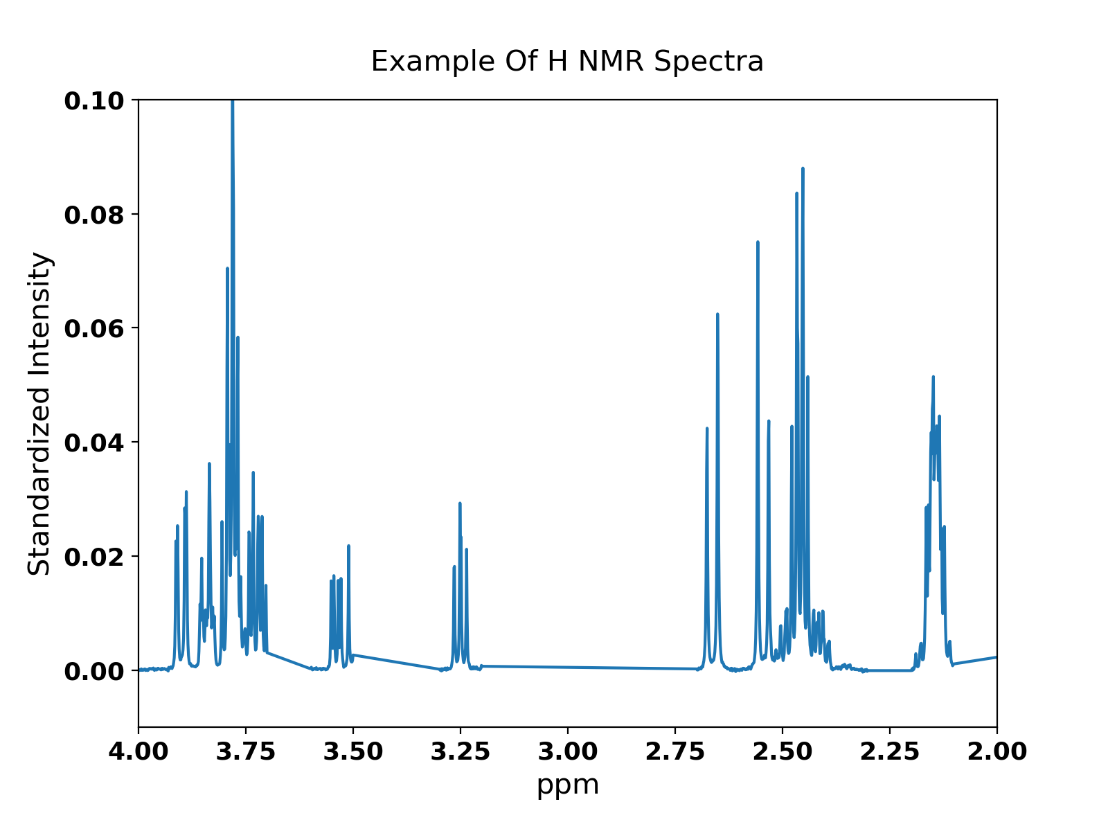
where $\gamma$ is the peak width at half height. An example of ¹H NMR spectrum is shown in Figure 7. The x-axis of the spectrum measures chemical shift in parts per million (ppm) and corresponds to the resonance frequency. The y-axis measures relative resonance intensity. Each spectrum peak corresponds to magnetic nuclei resonating at a particular frequency in the biological mixture, with every metabolite having a characteristic molecular ¹H NMR ‘signature’; the result is a convolution of Lorentzian peaks that appear in specific positions in ¹H NMR spectra. Each metabolite in the experiment usually gives rise to more than a ‘multiplet’ in the spectrum – i.e. linear combination of Lorentzian functions, symmetric around a central point. Spectral signature (i.e. pattern multiplets) of many metabolites are stored in public databases. The aim of the analysis is: (i) to deconvolve resonance peak in the spectrum and assign them to a particular metabolite; (ii) estimate the abundance of the catalogued metabolites; (iii) model the component of a spectrum that cannot be assigned to known compounds. Astle et al. 2012 propose a two-component joint model for a spectrum, in which the metabolites whose peaks we wish to assign explicitly are modelled parametrically, using information from the online databases, while the unassigned spectrum is modelled using wavelets.

4.1 The Model

We now describe the model of Astle et al. 2012. The available data are represented by the pair $(\mathbf{x},\mathbf{y})$ , where $\mathbf{x}$ is a vector of $n$ ordered points (of the order $10^{3}-10^{4}$ ) on the chemical shift axis – often regularly spaced – and $\mathbf{y}$ is the vector of the corresponding resonance intensity measurements (scaled, so that they sum up to $1$ ). The conditional law of $\mathbf{y}|\mathbf{x}$ is modelled under the assumption that $y_{i}|\mathbf{x}$ are independent normal variables and,

\mathbb{E}\,[\,y_{i}\,|\,\mathbf{x}\,]=\phi(x_{i})+\xi(x_{i}),\quad 1\leq i\leq n.

(15)

Here, the $\phi$ component of the model represents signatures that we wish to assign to target metabolites. The $\xi$ component models signatures of remaining metabolites present in the spectrum, but not explicitly modelled. We refer to this latter as residual spectrum and we highlight the fact that it is important to account for it as it can unveil important information not captured by $\phi(\cdot)$ . Function $\phi$ is constructed parametrically using results from the physical theory of NMR and information available online databases or expert knowledge, while $\xi$ is modelled semiparametrically with wavelets generated by a mother wavelet (symlet 6) that resembles the Lorentzian curve.

More analytically,

\phi(x_{i})=\sum_{m=1}^{M}t_{m}(x_{i})\beta_{m}

where $M$ is the number of metabolites modelled explicitly and $\beta=(\beta_{1},\ldots,\beta_{M})^{\top}$ is a parameter vector corresponding to metabolite concentrations. Function $t_{m}(\cdot)$ represents a continuous template function that specifies the NMR signature of metabolite $m$ and it is defined as,

t_{m}(\delta)=\sum_{u}\sum^{V_{m,u}}_{v=1}z_{m,u}\,\omega_{m,u,v}\,\ell_{\gamma}(\delta-\delta^{*}_{m,u}-c_{m,u,v}),\quad\delta>0,

(16)

where $u$ is an index running over all multiplets assigned to metabolite $m$ , $v$ is an index representing a peak in a multiplet and $V_{m,u}$ is the number of peaks in multiplet $u$ of metabolite $m$ . In addition, $\delta^{*}_{m,u}$ specifies the theoretical position on the chemical shift axis of the centre of mass of the $u$ th multiplet of the $m$ th metabolite; $z_{m,u}$ is a positive quantity, usually equal to the number of protons in a molecule of metabolite $m$ that contributes to the resonance signal of multiplet $u$ ; $\omega_{m,u,v}$ is the weight determining the relative heights of the peaks of the multiplet; $c_{m,u,v}$ is the translation determining the horizontal offsets of the peaks from the centre of mass of the multiplet. Both $\omega_{m,u,v}$ and $c_{m,u,v}$ can be computed by empirical estimates of the so-called $J$ -coupling constants; see Hore 2015 for more details. The $z_{m,u}$ ’s and $J$ -coupling constants information can be found in online databases or from expert knowledge.

The residual spectrum is modelled through wavelets,

\xi(x_{i})=\sum_{j,k}\varphi_{j,k}(x_{i})\vartheta_{j,k}

where $\varphi_{j,k}(\cdot)$ denote the orthogonal wavelet functions generated by the symlet-6 mother wavelet, see Astle et al. 2012 for full details; here, $\vartheta=(\vartheta_{1,1},\ldots,\vartheta_{j,k},\ldots)^{\top}$ is the vector of wavelet coefficients. Indices $j,k$ correspond to the $k$ th wavelet in the $j$ th scaling level.

Finally, overall, the model for an NMR spectrum can be re-written in matrix form as:

\mathcal{W}(\mathbf{y}-\mathbf{T}\beta)=\mathbf{I}_{n_{1}}\vartheta+\epsilon,\quad\boldsymbol{\epsilon}\sim\mathrm{N}(0,\mathbf{I}_{n_{1}}/\theta),

(17)

where $\mathcal{W}\in\mathbb{R}^{n\times{n_{1}}}$ is the inverse wavelet transform, $M$ is the total number of known metabolites, $\mathbf{T}$ is an $n\times M$ matrix with its $(i,m)$ th entry equal to $t_{m}(x_{i})$ and $\theta$ is a scalar precision parameter.

4.2 Prior Specification

Astle et al. 2012 assign the following prior distribution to the parameters in the Bayesian model. For the concentration parameters, we assume

\beta_{m}\sim\mathrm{TN}(e_{m},1/s_{m},0,\infty),

where $e_{m}=0$ and $s_{m}=10^{-3}$ , for all $m=1,\ldots,M$ . Moreover,

	$\displaystyle\gamma$	$\displaystyle\sim\mathrm{LN}(0,1);$
	$\displaystyle\delta^{*}_{m,u}$	$\displaystyle\sim\mathrm{TN}(\hat{\delta}^{}_{m,u},10^{-4},\hat{\delta}^{}_{m,u}-0.03,\hat{\delta}^{*}_{m,u}+0.03),$

where LN denotes a log-normal distribution and $\hat{\delta}^{*}_{m,u}$ is the estimate for $\delta^{*}_{m,u}$ obtained from the online database HMDB (Wishart et al. 2017; Wishart et al. 2012; Wishart et al. 2008; Wishart et al. 2007, see). In the regions of the spectrum where both parametric (i.e. $\phi$ ) and semiparametric (i.e. $\xi$ ) components need to be fitted, the likelihood is unidentifiable. To tackle this problem, Astle et al. 2012 opt for shrinkage priors for the wavelet coefficients and include a vector of hyperparameters $\psi$ – each component $\psi_{j,k}$ of which corresponds to a wavelet coefficient – to penalize the semiparametric component. To reflect prior knowledge that NMR spectra are usually restricted to the half plane above the chemical shift axis, Astle et al. 2012 introduce a vector of hyperparameters $\tau$ , each component of which, $\tau_{i}$ , corresponds to a spectral data point, to further penalize spectral reconstructions in which some components of $\mathcal{W}^{-1}\boldsymbol{\vartheta}$ are less than a small negative threshold. In conclusion, Astle et al. 2012 specify the following joint prior density for $(\vartheta,\psi,\tau,\theta)$ ,

	$\displaystyle p(\vartheta,\psi,\tau,\theta)$	$\displaystyle\propto\theta^{a+\tfrac{n+n_{1}}{2}-1}\Big\{\prod_{j,k}\psi^{c_{j}-0.5}_{j,k}\exp\big(-\tfrac{\psi_{j,k}d_{j}}{2}\big)\Big\}$
		$\displaystyle\qquad\qquad\times\exp\Big\{-\tfrac{\theta}{2}\Big(e+\sum_{j,k}\psi_{j,k}\,\vartheta^{2}_{j,k}+r\sum^{n}_{i=1}(\tau_{i}-h)^{2}\Big)\Big\}$
		$\displaystyle\qquad\qquad\qquad\qquad\times\mathbbm{1}\,\big\{\,\mathcal{W}^{-1}\vartheta\geq\tau,\,\,h\mathbf{1}_{n}\geq\tau\,\big\},$

where $\psi$ introduces local shrinkage for the marginal prior of $\vartheta$ and $\tau$ is a vector of $n$ truncation limits, which bounds $\mathcal{W}^{-1}\vartheta$ from below. The truncation imposes an identifiability constraint: without it, when the signature template does not match the shape of the spectral data, the mismatch will be compensated by negative wavelet coefficients, such that an ideal overall model fit is achieved even though the signature template is erroneously assigned and the concentration of metabolites is overestimated. Finally we set $c_{j}=0.05$ , $d_{j}=10^{-8}$ , $h=-0.002$ , $r=10^{5}$ , $a=10^{-9}$ , $e=10^{-6}$ ; see Astle et al. 2012 for more details.

4.3 Results

BATMAN is an $\mathsf{R}$ package for estimating metabolite concentrations from NMR spectral data using a specifically designed MCMC algorithm (Hao et al. 2012) to perform posterior inference from the Bayesian model described above. We implement a MC-CAVI version of BATMAN and compare its performance with the original MCMC algorithm. Details of the implementation of MC-CAVI are given in Appendix D. Due to the complexity of the model and the datasize, it is challenging for both algorithms to reach convergence. We run the two methods, MC-CAVI and MCMC, for approximately an equal amount of time, to analyse a full spectrum with 1,530 data points and modelling parametrically 10 metabolites. We fix the number of iterations for MC-CAVI to 1,000, with a burn-in of 500 iterations; we set the Monte Carlo size to $N=10$ for all iterations. The execution time for this MC-CAVI algorithms is $2,048$ secs. For the MCMC algorithm, we fix the number of iterations to 2,000, with a burn-in of 1,000 iterations. This MCMC algorithm has an execution time of $2,098$ secs.

In ¹H NMR analysis, $\beta$ (the concentration of metabolites in the biofluid) and $\delta^{*}_{m,u}$ (the peak positions) are the most important parameters from a scientific point of view. Traceplots of four examples ( $\beta_{3}$ , $\beta_{4}$ , $\beta_{9}$ and $\delta_{4,1}$ ) are shown in Figure 8. These four parameters are chosen due to the different performance of the two methods, which are closely examined in Figure 10. For $\beta_{3}$ and $\beta_{9}$ , traceplots are still far from convergence for MCMC, while they move toward the correct direction (see Figure 8) when using MC-CAVI. For $\beta_{4}$ and $\delta_{4,1}$ , both parameters reach a stable regime very quickly in MC-CAVI, whereas the same parameters only make local moves when implementing MCMC. For the remaining parameters in the model, both algorithms present similar results.

Figure 9 shows the fit obtained from both the algorithms, while Table 3 reports posterior estimates for $\beta$ . From Figure 9, it is evident that the overall performance of MC-CAVI is similar as that of MCMC since in most areas, the metabolites fit (orange line) captures the shape of the original spectrum quite well. Table 3 shows that, similar to standard VI behaviour, MC-CAVI underestimates the variance of the posterior density. We examine in more detail the posterior distribution of the $\beta$ coefficients for which the posterior means obtained with the two algorithms differ more than 1.0e-4. Figure 10 shows that MC-CAVI manages to capture the shapes of the peaks while MCMC does not, around ppm values of 2.14 and 3.78, which correspond to spectral regions where many peaks overlap making peak deconvolution challenging. This is probably due to the faster convergence of MC-CAVI. Figure 10 shows that for areas with no overlapping (e.g. around ppm values of 2.66 and 7.53), MC-CAVI and MCMC produce similar results.

		$\beta_{1}$	$\beta_{2}$	$\boldsymbol{\beta_{3}}$	$\boldsymbol{\beta_{4}}$	$\beta_{5}$
MC-CAVI	mean	6.0e-6	7.8e-5	1.4e-3	4.2e-4	2.6e-5
MC-CAVI	sd	1.8e-11	4.0e-11	1.3e-11	1.0e-11	6.2e-11
MCMC	mean	1.2e-5	4.0e-5	1.5e-3	2.1e-5	3.4e-5
MCMC	sd	1.1e-10	5.0e-10	1.6e-9	6.4e-10	3.9e-10
		$\beta_{6}$	$\beta_{7}$	$\beta_{8}$	$\boldsymbol{\beta_{9}}$	$\beta_{10}$
MC-CAVI	mean	6.1e-4	3.0e-5	1.9e-4	2.7e-3	1.0e-3
MC-CAVI	sd	1.5e-11	1.6e-11	3.9e-11	1.6e-11	3.6e-11
MCMC	mean	6.0e-4	3.0e-5	1.8e-4	2.5e-3	1.0e-3
MCMC	sd	2.3e-10	7.5e-11	3.7e-10	5.1e-9	7.9e-10

Table 3: Estimation of

\beta

obtained with MC-CAVI and MCMC. (The coefficients of

\beta

for which the posterior means obtained with the two algorithms differ by more than 1.0e-4 are shown in bold.)

Comparing MC-CAVI and MCMC’s performance in the case of the NMR model, we can draw the following conclusions:

•

In NMR analysis, if many peaks overlap (see Figure 10), MC-CAVI can provide better results than MCMC.
•

In high-dimensional models, where the number of parameters grows with the size of data, MC-CAVI can converge faster than MCMC.
•

Choice of $N$ is important for optimising the performance of MC-CAVI. Building on results derived for other Monte Carlo methods (e.g. MCEM), it is reasonable to choose a relatively small number of Monte Carlo iterations at the beginning when the algorithm can be far from regions of parameter space of high posterior probability, and gradually increase the number of Monte Carlo iterations, with the maximum number taken once the algorithm has reached a mode.

5 Discussion

As a combination of VI and MCMC, MC-CAVI provides a powerful inferential tool particularly in high dimensional settings when full posterior inference is computationally demanding and the application of optimization and of noisy-gradient-based approaches, e.g. BBVI, is hindered by the presence of hard constraints. The MCMC step of MC-CAVI is necessary to deal with parameters for which VI approximation distributions are difficult or impossible to derive, for example due to the impossibility to derive closed-form expression for the normalising constant. General Monte Carlo algorithms such as sequential Monte Carlo and Hamiltonian Monte Carlo can be incorporated within MC-CAVI. Compared with MCMC, the VI step of MC-CAVI speeds up convergence and provides reliable estimates in a shorter time. Moreover, MC-CAVI scales better in high-dimensional settings. As an optimization algorithm, MC-CAVI’s convergence monitoring is easier than MCMC. Moreover, MC-CAVI offers a flexible alternative to BBVI. This latter algorithm, although very general and suitable for a large range of complex models, depends crucially on the quality of the approximation to the true target provided by the variational distribution, which in high dimensional setting (in particular with hard constraints) is very difficult to assess.

Acknowledgments

We thank two anonymous referees for their comments that greatly improved the content of the paper. AB acknowledges funding by the Leverhulme Trust Prize.

Appendix A Proof of Lemma 1

Proof.

Part (i): For a neighborhood of $\lambda^{*}$ , we can chose a sub-neighborhood $V$ as described in Assumption 3. For some small $\epsilon>0$ , the set $V_{0}=\{\lambda:\textrm{ELBO}(q(\lambda))\geq\textrm{ELBO}(q(\lambda^{*}))-\epsilon\}$ has a connected component, say $V^{\prime}$ , so that $\lambda^{*}\in V^{\prime}$ and $V^{\prime}\subseteq V$ ; we can assume that $V^{\prime}$ is compact. Assumption 3 implies that $M(V^{\prime})\subseteq V_{0}$ ; in fact, since $M(V^{\prime})$ is connected and contains $\lambda^{*}$ , we have $M(V^{\prime})\subseteq V^{\prime}$ . This completes the proof of part (i) of Definition 1.
Part (ii): Let $\lambda\in V^{\prime}$ . Consider the sequence $\{M^{k}(\lambda)\}_{k}$ with a convergent subsequence, $M^{a_{k}}(\lambda)\rightarrow\lambda_{1}\in V^{\prime}$ , for increasing integers $\{a_{k}\}$ . Thus, we have that the following holds, $\textrm{ELBO}(q(M^{a_{k+1}}(\lambda)))\geq\textrm{ELBO}(q(M(M^{a_{k}}(\lambda))))\rightarrow\textrm{ELBO}(q(M(\lambda_{1})))$ , whereas we also have that $\textrm{ELBO}(q(M^{a_{k+1}}(\lambda)))\rightarrow\textrm{ELBO}(q(\lambda_{1}))$ . These two last limits give the implication that $\textrm{ELBO}(q(M(\lambda_{1})))=\textrm{ELBO}(q(\lambda_{1}))$ , so that $\lambda_{1}=\lambda^{*}$ . We have shown that any convergent subsequence of $\{M^{k}(\lambda)\}_{k}$ has limit $\lambda^{*}$ ; the compactness of $V^{\prime}$ gives that also $M^{k}(\lambda)\rightarrow\lambda^{*}$ . This completes the proof of part (ii) of Definition 1. ∎

Appendix B Proof of Theorem 1

Proof.

Let $V_{1}$ be as $V^{\prime}$ within the proof of Lemma 1. Define $V_{2}=\{\lambda\in V_{1}:|\lambda-\lambda^{*}|\geq\epsilon\}$ , for an $\epsilon>0$ small enough so that $V_{1}\neq\emptyset$ . For $\lambda\in V_{2}$ , we have $M(\lambda)\neq\lambda$ , thus there are $\nu,\nu_{1}>0$ such that for all $\lambda\in V_{2}$ and for all $\lambda^{\prime}$ with $|\lambda^{\prime}-M(\lambda)|<\nu$ , we obtain that $\textrm{ELBO}(q(\lambda^{\prime}))-\textrm{ELBO}(q(\lambda))>\nu_{1}$ . Also, due to continuity and compactness, there is $\nu_{2}>0$ such that for all $\lambda\in V_{1}$ and for all $\lambda^{\prime}$ such that $|\lambda^{\prime}-M(\lambda)|<\nu_{2}$ , we have $\lambda^{\prime}\in V_{1}$ . Let $R=\sup_{\lambda,\lambda^{\prime}\in V_{1}}\{\textrm{ELBO}(q(\lambda))-\textrm{ELBO}(q(\lambda^{\prime}))\}$ and $k_{0}=[R/\nu_{1}]$ where $[\cdot]$ denotes integer part. Notice that given $\lambda^{k}_{N}:=\mathcal{M}_{N}^{k}(\lambda)$ , we have that $\{|\mathcal{M}^{k+1}_{N}-M(\lambda^{k}_{N})|<\nu_{2}\}\subseteq\{\lambda^{k+1}_{N}\in V_{1}\}$ . Consider the event $F_{N}=\{\lambda_{N}^{k}\in V_{1}\,;\,k=0,\ldots,k_{0}\}$ . Under Assumption 4, we have that $\mathrm{Prob}[F_{N}]\geq p^{k_{0}}$ for $p$ arbitrarily close to 1. Within $F_{N}$ , we have that $|\lambda_{N}^{k}-\lambda^{*}|<\epsilon$ for some $k\leq k_{0}$ , or else $\lambda_{N}^{k}\in V_{2}$ for all $k\leq k_{0}$ , giving that $\textrm{ELBO}(q(\lambda^{k}_{N}))-\textrm{ELBO}(q(\lambda))>\nu_{1}\cdot k_{0}>R$ , which is impossible. ∎

Appendix C Gradient Expressions for BBVI

	$\displaystyle\nabla_{\alpha_{\vartheta}}\log q(\vartheta)$	$\displaystyle=(\vartheta-\alpha_{\vartheta})\cdot\exp(-\gamma_{\vartheta}),$
	$\displaystyle\nabla_{\gamma_{\vartheta}}\log q(\vartheta)$	$\displaystyle=-\tfrac{1}{2}+\tfrac{(\vartheta-\alpha_{\vartheta})^{2}}{2}\cdot\exp(-\gamma_{\vartheta}),$
	$\displaystyle\nabla_{\alpha_{\theta}}\log q(\theta)$	$\displaystyle=\big(\gamma_{\theta}-\tfrac{\Gamma^{\prime}(\exp(\alpha_{\theta}))}{\Gamma(\exp(\alpha_{\theta}))}+\log(\theta)\big)\cdot\exp(\alpha_{\theta}),$
	$\displaystyle\nabla_{\gamma_{\theta}}\log q(\theta)$	$\displaystyle=\exp(\alpha_{\theta})-\theta\cdot\exp(\gamma_{\theta}),$
	$\displaystyle\nabla_{\alpha_{\kappa_{j}}}\log q(\kappa_{j},\psi_{j})$	$\displaystyle=\tfrac{\kappa_{j}-\alpha_{\kappa_{j}}}{\exp(2\gamma_{\kappa_{j}})}+\tfrac{\phi(\frac{\psi_{j}-\alpha_{\kappa_{j}}}{\exp(\gamma_{\kappa_{j}})})-\phi(\frac{-\psi_{j}-\alpha_{\kappa_{j}}}{\exp(\gamma_{\kappa_{j}})})}{\exp(\gamma_{\kappa_{j}})(\Phi(\frac{\psi_{j}-\alpha_{\kappa_{j}}}{\exp(\gamma_{\kappa_{j}})})-\Phi(\frac{-\psi_{j}-\alpha_{\kappa_{j}}}{\exp(\gamma_{\kappa_{j}})}))},\quad 1\leq j\leq{n}$
	$\displaystyle\nabla_{\alpha_{\psi_{j}}}\log q(\kappa_{j},\psi_{j})$	$\displaystyle=\tfrac{\psi_{j}-\alpha_{\psi_{j}}}{\exp(2\gamma_{\psi_{j}})}+\tfrac{\phi(\frac{2-\alpha_{\psi_{j}}}{\exp(\gamma_{\psi_{j}})})-\phi(\frac{-\alpha_{\psi_{j}}}{\exp(\gamma_{\psi_{j}})})}{\exp(\gamma_{\psi_{j}})(\Phi(\frac{2-\alpha_{\psi_{j}}}{\exp(\gamma_{\psi_{j}})})-\Phi(\frac{-\alpha_{\psi_{j}}}{\exp(\gamma_{\psi_{j}})}))},\quad 1\leq j\leq{n}$
	$\displaystyle\nabla_{\gamma_{\kappa_{j}}}\log q(\kappa_{j},\psi_{j})$	$\displaystyle=\tfrac{(\kappa_{j}-\alpha_{\kappa_{j}})^{2}}{\exp(2\gamma_{\kappa_{j}})}-1+\tfrac{(\psi_{j}-\alpha_{\kappa_{j}})\phi(\frac{\psi_{j}-\alpha_{\kappa_{j}}}{\exp(\gamma_{\kappa_{j}})})+(\psi_{j}+\alpha_{\kappa_{j}})\phi(\frac{-\psi_{j}-\alpha_{\kappa_{j}}}{\exp(\gamma_{\kappa_{j}})})}{\exp(\gamma_{\kappa_{j}})(\Phi(\frac{\psi_{j}-\alpha_{\kappa_{j}}}{\exp(\gamma_{\kappa_{j}})})-\Phi(\frac{-\psi_{j}-\alpha_{\kappa_{j}}}{\exp(\gamma_{\kappa_{j}})}))},\quad 1\leq j\leq{n}$
	$\displaystyle\nabla_{\gamma_{\psi_{j}}}\log q(\kappa_{j},\psi_{j})$	$\displaystyle=\tfrac{(\psi_{j}-\alpha_{\psi_{j}})^{2}}{\exp(2\gamma_{\psi_{j}})}-1+\tfrac{(2-\alpha_{\psi_{j}})\boldsymbol{\phi}(\frac{2-\alpha_{\psi_{j}}}{\exp(\gamma_{\psi_{j}})})+(\alpha_{\psi_{j}})\boldsymbol{\phi}(\frac{-\alpha_{\psi_{j}}}{\exp(\gamma_{\psi_{j}})})}{\exp(\gamma_{\psi_{j}})(\Phi(\frac{2-\alpha_{\psi_{j}}}{\exp(\gamma_{\psi_{j}})})-\Phi(\frac{-\alpha_{\psi_{j}}}{\exp(\gamma_{\psi_{j}})}))},\quad 1\leq j\leq{n}.$

Appendix D MC-CAVI Implementation of BATMAN

In the MC-CAVI implementation of BATMAN, taking both computation efficiency and model structure into consideration, we assume that the variational distribution factorises over four partitions of the parameter vectors, $q(\beta,\delta^{*},\gamma)$ , $q(\vartheta,\tau)$ , $q(\psi)$ , $q(\theta)$ . This factorization is motivated by the original Metropolis-Hastings block updates in Astle et al. 2012. Let $B$ denote the wavelet basis matrix defined by the transform $\mathcal{W}$ , so $\mathcal{W}(B)=\mathbf{I}_{n_{1}}$ . We use $v_{-i}$ to represent vector $v$ without the $i$ th component and analogous notation for matrices (resp., without the $i$ th column).

Set $\mathbb{E}(\theta)=2a/e$ , ${\mathbb{E}}(\vartheta^{2}_{j,k})=0$ , ${\mathbb{E}}(\vartheta)=0$ , ${\mathbb{E}}(\tau)=0$ , ${\mathbb{E}}(\mathbf{T}\beta)=\mathbf{y}$ , ${\mathbb{E}}\big((\mathbf{T}\beta)^{\top}(\mathbf{T}\beta)\big)=\mathbf{y}^{\top}\mathbf{y}$ .

For each iteration:

1.

Set $q(\psi_{j,k})=\mathrm{Gamma}\big(c_{j}+\frac{1}{2},\tfrac{{\mathbb{E}}(\theta)\mathbb{E}(\vartheta^{2}_{j,k})+d_{j}}{2}\big)$ ; calculate $\mathbb{E}(\psi_{j,k})$ .

Set $q(\theta)=\mathrm{Gamma}(c,c^{\prime})$ , where we have defined,

	$\displaystyle c$	$\displaystyle=a_{1}+n_{1}+\tfrac{n}{2},$
	$\displaystyle c^{\prime}$	$\displaystyle=\tfrac{1}{2}\Big\{\sum_{j,k}\mathbb{E}(\psi_{j,k})\mathbb{E}(\vartheta^{2}_{j,k})+\mathbb{E}\big((\mathcal{W}\mathbf{y}-\mathcal{W}\mathbf{T}\beta-\vartheta)^{\top}(\mathcal{W}\mathbf{y}-\mathcal{W}\mathbf{T}\beta-\vartheta)\big)$
		$\displaystyle\qquad\qquad\qquad\qquad\qquad\qquad\qquad+r(\mathbb{E}(\tau)-h\mathbf{1}_{n})+e\Big\};$

calculate $\mathbb{E}(\theta)$ .

Use Monte Carlo to draw $N$ samples from $q(\beta,\delta^{*}_{m,u},\gamma)$ , which is derived via (4) as,

	$\displaystyle q(\beta,\delta^{*},\gamma)$	$\displaystyle\propto\exp\Big\{-\tfrac{\mathbb{E}(\theta)}{2}\big((\mathcal{W}\boldsymbol{T}\beta)^{\top}\mathcal{W}\boldsymbol{T}\beta-2\mathcal{W}\boldsymbol{T}\beta(\mathcal{W}\mathbf{y}-{\mathbb{E}}(\vartheta))\big)\Big\}$
		$\displaystyle\qquad\qquad\qquad\qquad\qquad\qquad\times p(\beta)p(\delta^{*})p(\gamma),$

where $p(\beta)$ , $p(\delta^{*})$ , $p(\gamma)$ are the prior distributions specified in Section 4.2.

•

Use a Gibbs sampler update to draw samples from $q(\beta|\delta^{*}_{m,u},\gamma)$ . Draw each component of $\beta=(\beta_{m})$ from a univariate normal, truncated below at zero, with precision and mean parameters given, respectively, by

	$\displaystyle P:=s_{m}+{\mathbb{E}}(\theta)(\mathcal{W}\boldsymbol{T}_{i})^{\top}(\mathcal{W}\boldsymbol{T}_{i}),$
	$\displaystyle(\mathcal{W}\boldsymbol{T}_{i})^{\top}(\mathcal{W}\mathbf{y}-\mathcal{W}\boldsymbol{T}_{-i}\beta_{-i}-{\mathbb{E}}(\vartheta)){\mathbb{E}}(\theta)/P.$

•

Use Metropolis–Hastings to update $\gamma$ . Propose $\log(\gamma^{\prime})\sim\mathrm{N}(\log(\gamma),V_{\gamma}^{2})$ . Perform accept/reject. Adapt $V_{\gamma}^{2}$ to obtain average acceptance rate of approximately 0.45.

•

Use Metropolis–Hastings to update $\delta^{*}_{m,u}$ . Propose,

({\delta^{*}_{m,u}})^{\prime}\sim\mathrm{TN}(\delta^{*}_{m,u},V_{\delta^{*}_{m,u}}^{2},\hat{\delta}^{*}_{m,u}-0.03,\hat{\delta}^{*}_{m,u}+0.03).

Perform accept/reject. Adapt $V_{\delta^{*}_{m,u}}^{2}$ to target acceptance rate 0.45.

Calculate ${\mathbb{E}}(\mathbf{T}\beta)$ and ${\mathbb{E}}\big((\mathbf{T}\beta)^{\top}(\mathbf{T}\beta)\big)$ .

Use Monte Carlo to draw $N$ samples from $q(\vartheta,\tau)$ , which is derived via (4) as,

		$\displaystyle q(\vartheta,\tau)\propto$
		$\displaystyle\exp\Big\{-\tfrac{\mathbb{E}(\theta)}{2}\Big(\sum_{j,k}\vartheta_{j,k}\big((\psi_{j,k}+1)\,\vartheta_{j,k}-2\big(\mathcal{W}\mathbf{y}-\mathcal{W}\mathbb{E}(\boldsymbol{T}\beta)\big)_{j,k}\big)+r\sum^{n}_{i=1}(\tau_{i}-h)^{2}\Big)\Big\}$
		$\displaystyle\quad\quad\quad\quad\quad\quad\quad\quad\quad\quad\quad\quad\quad\quad\quad\quad\quad\times\mathbb{I}\,\big\{\,\mathcal{W}^{-1}\vartheta\geq\tau,\,\,h\mathbf{1}_{n}\geq\tau\,\big\}$

•

Use Gibbs sampler to draw from $q(\vartheta|\tau)$ . Draw $\vartheta_{j,k}$ from:

\mathrm{TN}\big(\tfrac{1}{1+\mathop{\mathbb{E}}(\psi_{j,k})}\big(\mathcal{W}\mathbf{y}-\mathcal{W}{\mathbb{E}}(\boldsymbol{T}\beta)\big)_{j,k},\tfrac{1}{{\mathbb{E}}(\theta)(1+{\mathbb{E}}(\psi_{j,k}))},L,U\big)

where we have set,

	$\displaystyle L$	$\displaystyle=\max_{i:B_{i\{j,k\}}>0}\frac{\tau_{i}-B_{i-\{j,k\}}\vartheta_{-\{j,k\}}}{B_{i\{j,k\}}}$
	$\displaystyle U$	$\displaystyle=\min_{i:B_{i\{j,k\}}<0}\frac{\tau_{i}-B_{i-\{j,k\}}\vartheta_{-\{j,k\}}}{B_{i\{j,k\}}}$

and $B_{i\{j,k\}}$ is the $(j,k)$ th element of the $i$ th column of $B$ .

•

Use Gibbs sampler to update $\tau_{i}$ . Draw,

$\tau_{i}\sim\mathrm{TN}\big(h,1/({\mathbb{E}}(\theta)r),-\infty,\min\big\{h,(\mathcal{W}^{-1}\vartheta)_{i}\big\}\big).$

Calculate ${\mathbb{E}}(\vartheta^{2}_{j,k})$ , ${\mathbb{E}}(\vartheta)$ , ${\mathbb{E}}(\tau)$ .

References

Astle et al. (2012) Astle, W., De Iorio, M., Richardson, S., Stephens, D., and Ebbels, T. (2012). A Bayesian model of NMR spectra for the deconvolution and quantification of metabolites in complex biological mixtures. Journal of the American Statistical Association, 107(500):1259–1271.
Beaumont et al. (2002) Beaumont, M. A., Zhang, W., and Balding, D. J. (2002). Approximate Bayesian computation in population genetics. Genetics, 162(4):2025–2035.
Bertsekas (1999) Bertsekas, D. P. (1999). Nonlinear programming. Athena scientific Belmont.
Bishop (2006) Bishop, C. M. (2006). Pattern recognition and machine learning. Springer.
Blei et al. (2017) Blei, D. M., Kucukelbir, A., and McAuliffe, J. D. (2017). Variational inference: A review for statisticians. Journal of the American Statistical Association, 112(518):859–877.
Booth and Hobert (1999) Booth, J. G. and Hobert, J. P. (1999). Maximizing generalized linear mixed model likelihoods with an automated Monte Carlo EM algorithm. Journal of the Royal Statistical Society: Series B (Statistical Methodology), 61(1):265–285.
Bottou (2012) Bottou, L. (2012). Stochastic Gradient Descent Tricks, pages 421–436. Springer Berlin Heidelberg, Berlin, Heidelberg.
Casella and Robert (1996) Casella, G. and Robert, C. P. (1996). Rao-Blackwellisation of sampling schemes. Biometrika, 83(1):81–94.
Chan and Ledolter (1995) Chan, K. and Ledolter, J. (1995). Monte Carlo EM estimation for time series models involving counts. Journal of the American Statistical Association, 90(429):242–252.
Duchi et al. (2011) Duchi, J., Hazan, E., and Singer, Y. (2011). Adaptive subgradient methods for online learning and stochastic optimization. Journal of Machine Learning Research, 12(Jul):2121–2159.
Forbes and Fort (2007) Forbes, F. and Fort, G. (2007). Combining Monte Carlo and mean-field-like methods for inference in hidden Markov random fields. IEEE Transactions on Image Processing, 16(3):824–837.
Fort et al. (2003) Fort, G., Moulines, E., et al. (2003). Convergence of the monte carlo expectation maximization for curved exponential families. The Annals of Statistics, 31(4):1220–1259.
Hao et al. (2012) Hao, J., Astle, W., De Iorio, M., and Ebbels, T. M. (2012). BATMAN–an R package for the automated quantification of metabolites from nuclear magnetic resonance spectra using a Bayesian model. Bioinformatics, 28(15):2088–2090.
Hoffman et al. (2013) Hoffman, M. D., Blei, D. M., Wang, C., and Paisley, J. (2013). Stochastic variational inference. The Journal of Machine Learning Research, 14(1):1303–1347.
Hore (2015) Hore, P. J. (2015). Nuclear magnetic resonance. Oxford University Press, USA.
Jordan et al. (1999) Jordan, M. I., Ghahramani, Z., Jaakkola, T. S., and Saul, L. K. (1999). An introduction to variational methods for graphical models. Machine learning, 37(2):183–233.
Kucukelbir et al. (2017) Kucukelbir, A., Tran, D., Ranganath, R., Gelman, A., and Blei, D. M. (2017). Automatic differentiation variational inference. The Journal of Machine Learning Research, 18(1):430–474.
Levine and Casella (2001) Levine, R. A. and Casella, G. (2001). Implementations of the Monte Carlo EM algorithm. Journal of Computational and Graphical Statistics, 10(3):422–439.
Ranganath et al. (2014) Ranganath, R., Gerrish, S., and Blei, D. (2014). Black box variational inference. In Artificial Intelligence and Statistics, pages 814–822.
Robbins and Monro (1951) Robbins, H. and Monro, S. (1951). A stochastic approximation method. Ann. Math. Statist., 22(3):400–407.
Ross (2002) Ross, S. M. (2002). Simulation. Elsevier.
Sisson et al. (2007) Sisson, S. A., Fan, Y., and Tanaka, M. M. (2007). Sequential Monte Carlo without likelihoods. Proceedings of the National Academy of Sciences, 104(6):1760–1765.
Tran et al. (2016) Tran, M.-N., Nott, D. J., Kuk, A. Y., and Kohn, R. (2016). Parallel variational Bayes for large datasets with an application to generalized linear mixed models. Journal of Computational and Graphical Statistics, 25(2):626–646.
Wainwright et al. (2008) Wainwright, M. J., Jordan, M. I., et al. (2008). Graphical models, exponential families, and variational inference, volume 1. Now Publishers, Inc.
Wei and Tanner (1990) Wei, G. C. and Tanner, M. A. (1990). A Monte Carlo implementation of the EM algorithm and the poor man’s data augmentation algorithms. Journal of the American statistical Association, 85(411):699–704.
Wishart et al. (2017) Wishart, D. S., Feunang, Y. D., Marcu, A., Guo, A. C., Liang, K., Vázquez-Fresno, R., Sajed, T., Johnson, D., Li, C., Karu, N., et al. (2017). HMDB 4.0: the human metabolome database for 2018. Nucleic acids research, 46(D1):D608–D617.
Wishart et al. (2012) Wishart, D. S., Jewison, T., Guo, A. C., Wilson, M., Knox, C., Liu, Y., Djoumbou, Y., Mandal, R., Aziat, F., Dong, E., et al. (2012). HMDB 3.0—the human metabolome database in 2013. Nucleic acids research, 41(D1):D801–D807.
Wishart et al. (2008) Wishart, D. S., Knox, C., Guo, A. C., Eisner, R., Young, N., Gautam, B., Hau, D. D., Psychogios, N., Dong, E., Bouatra, S., et al. (2008). HMDB: a knowledgebase for the human metabolome. Nucleic acids research, 37(suppl_1):D603–D610.
Wishart et al. (2007) Wishart, D. S., Tzur, D., Knox, C., Eisner, R., Guo, A. C., Young, N., Cheng, D., Jewell, K., Arndt, D., Sawhney, S., et al. (2007). HMDB: the human metabolome database. Nucleic acids research, 35(suppl_1):D521–D526.

	$\displaystyle q_{k-1}(\psi_{j}\|\kappa_{j})$	$\displaystyle\propto\frac{\phi(\tfrac{\psi_{j}-\frac{1}{20}}{\sqrt{10}})}{\Phi(\tfrac{\psi_{j}}{\sqrt{10}})-\Phi(\tfrac{-\psi_{j}}{\sqrt{10}})}\,\mathbb{I}\,[\,\|\kappa_{j}\|<\psi_{j}<2\,],$
	$\displaystyle q_{k-1}(\kappa_{j}\|\psi_{j})$	$\displaystyle=\mathrm{TN}\big(\tfrac{(y_{j}-\mathbb{E}_{k-1}(\vartheta))\mathbb{E}_{k-1}(\theta)}{\frac{1}{10}+\mathbb{E}_{k-1}(\theta)},\tfrac{1}{\frac{1}{10}+\mathbb{E}_{k-1}(\theta)},-\psi_{j},\psi_{j}\big).$

Monte Carlo Co-Ordinate Ascent Variational Inference

Abstract

1 Introduction

Remark 1 (Hard Constraints).

Remark 2.

2 MC-CAVI Algorithm

2.1 Description of the Algorithm

2.2 Applicability of MC-CAVI

2.3 Theoretical Justification of MC-CAVI

Assumption 1 (Closedness of Parameterised q⁡(⋅)q(\cdot) Under Variational Update).

Assumption 2.

Assumption 3 (Properties of M⁡(⋅)M(\cdot) Near a Local Maximum).

Assumption 4 (Uniform Convergence in Probability on Compact Sets).

Definition 1.

Lemma 1.

Theorem 1.

2.4 Stopping Criterion and Sample Size

Principled - but Impractical - Approach

Practical Considerations

3 Numerical Examples – Simulation Study

3.1 Simulated Example 1

3.2 Variance Reduction for BBVI

3.3 Simulated Example 2: Model with Hard Constraints

MCMC

MC-CAVI

BBVI

Results

4 Application to 1H NMR Spectroscopy

4.1 The Model

4.2 Prior Specification

4.3 Results

5 Discussion

Acknowledgments

Appendix A Proof of Lemma 1

Proof.

Appendix B Proof of Theorem 1

Proof.

Appendix C Gradient Expressions for BBVI

Appendix D MC-CAVI Implementation of BATMAN

References

Assumption 1 (Closedness of Parameterised $q(\cdot)$ Under Variational Update).

Assumption 3 (Properties of $M(\cdot)$ Near a Local Maximum).

4 Application to ¹H NMR Spectroscopy