Compositional Coding for Collaborative FilteringDOI: 10.475/123_4ISBN: 123-4567-24-567/08/06Conference: SIGIR; 2019; July 2019, Paris, France4Price: 15.00Note: Jianling Sun is the corresponding author.CCS: Information systems Recommender SystemCCS: Humancentered computing Collaborative filtering

Matrix Factorization (MF) is the most successful and widely used CF based recommendation method. It represents users and items with real-valued vectors. Then an interaction of the corresponding user and item can be efficiently estimated by the inner product. Formally, given a user-item interaction matrix $\mathbf{R}\in\mathbb{R}^{m\times n}$ with $m$ users and $n$ items. Let $\mathbf{u}_{i}\in\mathbb{R}^{r}$ and $\mathbf{v}_{j}\in\mathbb{R}^{r}$ denote the latent vector for user $i$ and item $j$ respectively. Then, the predicted preference of user $i$ towards item $j$ is formulated as $\hat{r}_{ij}=\mathbf{u}_{i}^{\top}\mathbf{v}_{j}.$ To learn all user latent vectors $\mathbf{U}=[\mathbf{u}_{1},\dots,\mathbf{u}_{m}]^{\top}\in\mathbb{R}^{m\times r}$ and item latent vectors $\mathbf{V}=[\mathbf{v}_{1},\dots,\mathbf{u}_{n}]^{\top}\in\mathbb{R}^{n\times r}$, MF minimizes the following regularized squared loss on the observed ratings:

where $\mathcal{V}$ denotes the all observed use-item pairs and $R(\mathbf{U},\mathbf{V})$ is the regularization term with respect to $\mathbf{U}$ and $\mathbf{V}$ controlled by $\lambda>0$. To improve recommendation efficiency, after we obtain the optimized user/item real-valued latent vectors, the two-stage hashing method use binary quantization (rounding off (Zhang et al. 2014) or rotate (Zhou and Zha 2012; Liu et al. 2014a)) to convert the continuous latent representations into binary codes. Let us denote $\mathbf{B}=[\mathbf{b}_{1},\dots,\mathbf{b}_{m}]^{\top}\in\{\pm 1\}^{m\times r}$ and $\mathbf{D}=[\mathbf{d}_{1},\dots,\mathbf{d}_{n}]^{\top}\in\{\pm 1\}^{n\times r}$ respectively as $r$-length user/item binary codes, then the inner product between the binary codes of user and item can be formulated as $\mathbf{b}_{i}^{\top}\mathbf{d}_{j}=2H(\mathbf{b}_{i},\mathbf{d}_{j})-r,$where $H(\cdot)$ denotes the Hamming similarity. Based on fast bit operations, Hamming distance computation is extremely efficient. However, this method usually incurs a large quantization error since the binary bits are obtained by thresholding real values to integers, and thus it cannot preserve the original data geometry in the continuous vector space (Zhang et al. 2016).

To circumvent the above issues, direct discrete optimization method has been proposed in Discrete Collaborative Filtering (DCF) (Zhang et al. 2016) and its extension (Lian et al. 2017; Zhang et al. 2017; Liu et al. 2018). More formally, it learns the binary codes by optimizing the following objective function:

This objective function is similar to that of a conventional MF task, except the discrete constraint on the user/item embeddings. By additionally imposing balanced and de-correlated constraints, it could derive compact yet informative binary codes for both users and items.

However, compared to real-valued vectors, CF with binary codes naturally suffers from low accuracy due to limited representation capability in each bit. Specifically, the $r$-dimensional real-valued vector space have infinite possibility to model users and items, while the number of unique binary codes in Hamming space is $2^{r}$. An alternative way to resolve this issue is to use a longer code. Unfortunately, it will adversely hurt the generalization of the model especially in the sparse scenarios.

In this work, we attempt to improve the efficiency of CF without hurting the prediction performance. We propose a new user/item representation named “Compositional Coding", which utilizes both the accuracy of real-valued vectors and the efficiency of binary codes to represent users and items. Since the fixed distance between each pair of binary codes impedes them from modeling different magnitudes of relationships between users and items, we assign real-valued weight to each bit to remarkably enrich their representation capability. Besides, the importance parameters could implicitly prune unimportant bits by setting their importance parameters close to $0$, which naturally reduces the computation cost.

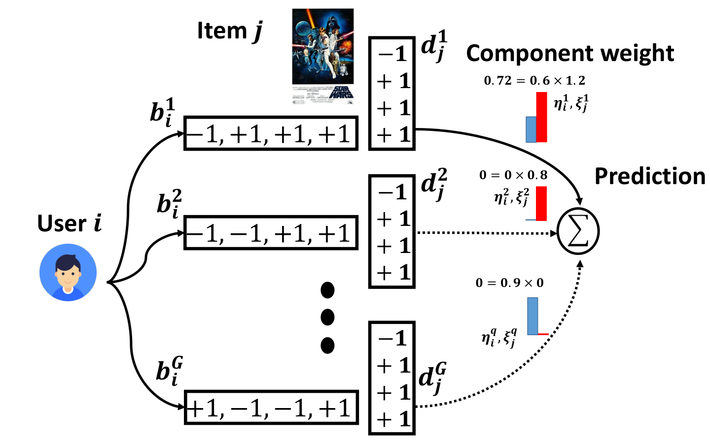
In general, the proposed compositional coding framework assumes each user or item is represented by $G$ components of $r$-dimensional binary codes ($r$ is relatively small) and one $G$-dimensional sparse weight vector. Formally, denote by

the compositional codes for the $i$-th user, and

the compositional codes for the $j$-th item, respectively. Then the predicted preference of user $i$ for item $j$ is computed by taking the weighted sum of the inner product with respect to each of the $G$ components:

where $w_{ij}^{(k)}=\eta_{i}^{(k)}\cdot\xi_{j}^{(k)}$ is the importance weight of the $k$-th component of binary codes with respect to user $i$ and item $j$.

Figure 2 illustrates how to estimate a user-item interaction using compositional codes. The inner product of each component of binary codes $(\mathbf{b}_{i}^{(k)})^{\top}\mathbf{d}_{j}^{(k)}$ can be efficiently computed in Hamming space using fast bit operations. The importance weight of the $k$-th component of binary codes $w_{ij}^{(k)}$ is obtained through a multiplication operation over $\eta_{i}^{(k)}$ and $\xi_{j}^{(k)}$, which ensures that the importance weight will be assigned a high value if and only if both user and item weights are large and will become zero if either of them is zero. It is worth noting that we use the multiplication instead of addition operation over the user and item weight to achieve the high sparsity of the sparse weight vector, which can lead to a significant reduction of computation cost during online recommendation.

Compared to representing users/items with binary codes, the key advantage of the proposed framework is that the sparse real-valued weight vector substantially increases the representation capacity of user/item embeddings by the compositional coding scheme. Recalling the example shown in Figure 1, we can preserve the movie relations by assigning them with different weight vectors, so as to predict user-item interactions with a lower error. Another benefit is mainly from the idea of compositional matrix approximation (Lee et al. 2013; Zhang et al. 2013), which is more suitable for real-world recommender systems, since the interaction matrix is very large and composed of diverse interaction behaviours. Under this view, the proposed compositional coding framework is characterized by multiple components of binary codes. Each component of binary codes can be employed to discover the localized relationships among certain types of similar users and items and thus can be more accurate in this particular region (e.g., young people viewing action movies while old people viewing romance movies). Therefore, the proposed compositional coding framework can encode users and items in a more informative way.

In addition to the improved representation and better accuracy, the compositional coding framework does not lose the high efficiency advantage of binary codes, and can even gain more efficiency when imposing sufficient sparsity. In order to show this, we analyze the time cost of the proposed framework and compare it against the conventional binary coding framework. In particular, assume the time cost of calculating the Hamming distance of $r$-bit codes is $T_{h}$ and the time cost of weighted summation of all of inner product results is $T_{s}$, then the total cost for a user-item similarity search is

where $nnz(\mathbf{w})$ denotes the average number of non-zero values in component weight vector $\mathbf{w}\in\mathbb{R}^{G}$, which is much smaller than $G$ in our approach due to the sparsity of the user and item weights. Similarly, the cost by conventional hashing based CF models using $(G\times r)$-bit binary codes is $G\times T_{h}$ which can be higher than ours.

Remark. The proposed compositional coding framework is rather general. When identical weight vectors are used, it is degraded to the binary codes of conventional hashing based CF methods. Compositional codes could also be regarded as real-valued latent vectors of CF model, if we adopt the identical binary codes for each component. In summary, compositional code is a flexible representation which could benefit from both the strong representation capability of real-valued vectors and the fast similarity search of binary codes.

In this section, we instantiate the compositional coding framework on Matrix Factorization (MF) models and term the proposed method as the Compositional Coding for Collaborative Filtering (CCCF). Note that the proposed compositional coding framework can be potentially applicable to other types of CF models beyond MF.

Follow the intuition of compositional coding, we assume that there exists a distance function $d$ that measures distances in the space of users ($i=1,\dots,m$) or items ($j=1,\dots,n$). The distance function leads to the notion of neighborhoods of user-user and item-item pairs. Its assumption states that the rating of user-item pair $(i,j)$ could be approximated particularly well in its neighbourhood. Thus, we identify $G$ components surrounding $K$ anchor points $(i^{\prime}_{1},j^{\prime}_{1}),\dots,(i^{\prime}_{G},j^{\prime}_{G})$. Follow the setting of compositional matrix approximation (Lee et al. 2013; Lee et al. 2014), user weight $\eta^{(k)}_{i}$ can be instantiated with an Epanechnikov kernel¹¹ 1 Similar to (Lee et al. 2014), we also tried uniform and triangular kernel, but the performance was worse than Epanechnikov kernel, in agreement with the theory of kernel smoothing (Wand and Jones 1994). (Wand and Jones 1994), which is formulated as:

where $h>0$ is a bandwidth parameter, $\bf{1}[\cdot]$ is the indicator function and $d(\cdot)$ is a distance function to measure the similarity between $i$ and $i^{\prime}_{t}$ (we will discuss it in Section 3.6). A large value of $h$ implies that $\bm{\eta}_{i}$ has a wide spread, which means most of the user component weights are non-zero. In contrast, a small $h$ corresponds to narrow spread of $\bm{\eta}_{i}$ and most of the user components will be zero. Item weight $\xi^{(k)}_{j}$ follows the analogous formulation. In this way, we could endow the weight vector $w^{(k)}_{ij}$ for user-item pair, which is defined as multiplication over user and item weight, with the sparsity. The method for selecting anchor points for each component is important as it may affect the values of component weights and further affect the generalization performance. A natural way is to uniformly sample them from the training set. In this work, we run $k$-means clustering with the user/item latent vectors and use the $G$ centroids as anchor points.

To learn the compositional codes, we adopt the squared loss to measure the reconstruction error as the standard MF method. For each set of binary codes, in order to maximize the entropy of each bit and make it as independent as possible, we impose balanced partition and decorrelated constraints. In summary, learning the compositional codes for users and items can be formulated into the following optimization task:

where we denote $\mathbf{B}^{(k)}=[\mathbf{b}^{(k)}_{1},\dots,\mathbf{b}^{(k)}_{m}]^{\top}\in\{\pm 1\}^{m\times r}$ and $\mathbf{D}^{(k)}=[\mathbf{d}^{(k)}_{1},\dots,\mathbf{d}^{(k)}_{n}]^{\top}\in\{\pm 1\}^{n\times r}$ respectively as user and item binary codes in the $k$-th set of binary codes. The problem formulated in (3.3) is a mixed-binary-integer program which is a challenging task since it is generally NP-hard and involves a combinatorial search over $O(2^{Gr(m+n)})$. An alternative way is to impose auxiliary continuous variables $\mathbf{X}^{(k)}\in\mathcal{B}$ and $\mathbf{Y}^{(k)}\in\mathcal{D}$ for each set of binary codes, where $\mathcal{B}^{(k)}=\{\mathbf{X}^{(k)}\in\mathcal{R}^{m\times r}|\textbf{1}_{m}\mathbf{X}^{(k)}=0,(\mathbf{X}^{(k)})^{\top}\mathbf{X}^{(k)}=m\mathbf{I}_{r}\}$ and $\mathcal{D}^{(k)}=\{\mathbf{Y}^{(k)}\in\mathcal{R}^{n\times r}|\textbf{1}_{n}\mathbf{Y}^{(k)}=0,(\mathbf{Y}^{(k)})^{\top}\mathbf{Y}^{(k)}=n\mathbf{I}_{r}\}$. Then the balanced and de-correlated constraints can be softened by $\min_{\mathbf{X}^{(k)}\in\mathcal{B}^{(k)}}\|\mathbf{B}^{(k)}-\mathbf{X}^{(k)}\|_{F}$ and $\min_{\mathbf{Y}^{(k)}\in\mathcal{D}^{(k)}}\|\mathbf{D}^{(k)}-\mathbf{Y}^{(k)}\|_{F}$, respectively. Finally, we can solve problem (3.3) with respect to the $k$-the set of codes in a computationally tractable manner:

where $\alpha_{1}$ and $\alpha_{2}$ are tuning parameters. Since $\text{tr}((\mathbf{B}^{(k)})^{\top}\mathbf{B}^{(k)})=\text{tr}((\mathbf{X}^{(k)})^{\top}\mathbf{X}^{(k)})=mr,$ and $\text{tr}((\mathbf{D}^{(k)})^{\top}\mathbf{D}^{(k)})=\text{tr}((\mathbf{Y}^{(k)})^{\top}\mathbf{Y}^{(k)})=nr,$ the above optimization task can be turned into the following

which is the proposed learning model for CCCF. Note that we do not discard the binary constraints but directly optimize the binary codes of each component. Through joint optimization for the binary codes and the auxiliary real-valued variables, we can achieve nearly balanced and un-correlated binary codes. Next, we will introduce an efficient solution for the mixed-integer optimization problem in Eq. (3.3).

We employ alternative optimization strategy to solve the above problem. Each iteration alternatively updates $\mathbf{B}^{(k)}$, $\mathbf{D}^{(k)}$, $\mathbf{X}^{(k)}$ and $\mathbf{Y}^{(k)}$. The details are given below.

Learning $\mathbf{B}^{(k)}$ and $\mathbf{D}^{(k)}$: In this subproblem, we update $\mathbf{B}^{(k)}$ with fixed $\mathbf{D}^{(k)}$, $\mathbf{X}^{(k)}$ and $\mathbf{Y}^{(k)}$. Since the objective function in Eq. (3.3) is based on summing over users of each component independently, so we can update binary codes for each user and item in parallel. Specifically, learning binary codes for user $i$ with respect to component $k$ is to solve the following optimization problem:

where $\tilde{r}_{ij}=r_{ij}-\sum_{\tilde{k}\neq k}w_{ij}^{\tilde{k}}(\mathbf{b}_{i}^{\tilde{k}})^{\top}\mathbf{d}_{j}^{\tilde{k}}$ is the residual of observed rating excluding the inner product of component $k$.

Due to the discrete constraints, the optimization is generally NP-hard, we adopt the bitwise learning method called Discrete Coordinate Descent (Shen et al. 2015; Shen et al. 2017) to update $\mathbf{b}^{(k)}_{i}$. In particular, denoting $b^{(k)}_{iq}$ as the $q$th bit of $\mathbf{b}^{(k)}_{i}$ and $\mathbf{b}^{(k)}_{i\bar{q}}$ as the rest codes excluding $b^{(k)}_{iq}$, DCD update $b^{(k)}_{iq}$ while fixing $\mathbf{b}^{(k)}_{i\bar{q}}$. Thus, the updating rule for user binary code $b^{(k)}_{iq}$ can be formulated as

where $\hat{b}^{(k)}_{iq}=\sum_{j\in\mathcal{V}_{i}}(\tilde{r}_{ij}-(w_{ij}^{(k)})^{2}(\mathbf{d}^{(k)}_{j\bar{q}})^{\top}\mathbf{b}^{(k)}_{i\bar{q}})d^{(k)}_{jq}+\alpha_{1}x^{(k)}_{iq}$, $\mathbf{d}^{(k)}_{j\bar{q}}$ is the rest set of item codes excluding $d_{jk}$ and $O(x,y)$ is a function that $O(x,y)=x$ if $x\neq 0$ and $O(x,y)=y$ otherwise. We iteratively update each bit until the procedure convergence. Note that the computational complexity of updating $\mathbf{B}^{(k)}$ is $O\big(\#iter(mnr^{2})\big)$ which is a critical efficiency bottleneck when $m$ or $n$ is large. To efficiently compute $\hat{b}^{(k)}_{iq}$, we rewrite $\hat{b}^{(k)}_{iq}$ as

which reduces the computational cost to $O\big(\#iter(m+n)r^{2}\big)$.

Similarly, we could learn binary code for item $j$ in component $k$ by solving

Denote $d^{(k)}_{jq}$ as the $q$-th bit of $\mathbf{d}^{(k)}_{j}$ and $\mathbf{d}^{(k)}_{j\bar{q}}$ as the rest codes excluding $d^{(k)}_{jq}$, we update each bit of $\mathbf{d}^{(k)}_{j}$ according to

where $\hat{d}^{(k)}_{jq}=\sum_{i\in\mathcal{V}_{j}}(\tilde{r}_{ij}-(w_{ij}^{(k)})^{2}(\mathbf{b}^{(k)}_{i\bar{q}})^{\top}\mathbf{d}^{(k)}_{j\bar{q}})b^{(k)}_{iq}+\alpha_{2}y^{(k)}_{jq}$.

Learning $\mathbf{X}^{(k)}$ and $\mathbf{Y}^{(k)}$: When fixing $\mathbf{B}^{(k)}$, learning $\mathbf{X}^{(k)}$ could be solved via optimizing the following objective function:

It can be solved by the aid of SVD according to (Liu et al. 2014b). Let $\bar{\mathbf{B}}^{(k)}$ be a column-wise zero-mean matrix, where $\bar{B}^{(k)}_{ij}=B^{(k)}_{ij}-\frac{1}{m}\sum_{i}B^{(k)}_{ij}$. Assuming $\bar{\mathbf{B}}^{(k)}=\mathbf{P}^{(k)}_{b}\bm{\Sigma}^{(k)}_{b}(\mathbf{Q}^{(k)}_{b})^{\top}$ as its SVD, where each column of $\mathbf{P}^{(k)}_{b}\in\mathbb{R}^{m\times r^{\prime}}$ and $\mathbf{Q}^{(k)}_{b}\in\mathbb{R}^{r\times r^{\prime}}$ represents the left and right singular vectors corresponding to $r^{\prime}$ non-zero singular values in the diagonal matrix $\bm{\Sigma}^{(k)}_{b}$. Since $\bar{\mathbf{B}}^{(k)}$ and $\mathbf{Q}^{(k)}_{b}$ have the same row, we have $\textbf{1}^{\top}{\mathbf{P}^{(k)}}_{b}=0$ due to $\textbf{1}^{\top}\bar{\mathbf{B}}^{(k)}=0$. Then we construct matrices $\hat{\mathbf{P}}^{(k)}_{b}$ of size $m\times(r-r^{\prime})$ and $\hat{\mathbf{Q}}^{(k)}_{b}$ of size $r\times(r-r^{\prime})$ by employing a Gram-Schmidt process such that $(\ \hat{\mathbf{P}}^{(k)})_{b}^{\top}\hat{\mathbf{P}}^{(k)}_{b}=\textbf{I}_{r-r^{\prime}}$, $[\mathbf{P}^{(k)}_{b}\textbf{ 1}]^{\top}\hat{\mathbf{P}}^{(k)}_{b}=0$, and $(\hat{\mathbf{Q}}^{(k)}_{b})^{\top}\hat{\mathbf{Q}}_{b}=\textbf{I}_{r-r^{\prime}}$, $[\mathbf{Q}^{(k)}_{b}\textbf{ 1}]^{\top}\hat{\mathbf{Q}}^{(k)}_{b}=0$. Now we obtain a closed-form update rule for $\mathbf{X}^{(k)}$:

In practice, to compute such an optimal $\mathbf{X}^{(k)}$, we perform the eigendecomposition over the small $r\times r$ matrix

which provides $\mathbf{Q}^{(k)}_{b},\hat{\mathbf{Q}}^{(k)}_{b},\bm{\Sigma}^{(k)}$, and we can obtain

Then matrix $\hat{\mathbf{P}}^{(k)}_{b}$ can be obtained by the aforementioned Gram-Schmidt orthogonalization. Note that it requires $O\big(r^{2}m\big)$ to perform SVD, Gram-Schimdt orthogonalization and matrix multiplication.

When $\mathbf{D}^{(k)}$ fixed, learning $\mathbf{Y}^{(k)}$ could be solved in a similar way:

We can obtain an analytic solution:

where each column of $\mathbf{P}^{(k)}_{d}$ and $\mathbf{Q}^{(k)}_{d}$ is the left and right singular vectors of $\bar{\mathbf{D}}^{(k)}$ respectively. $\hat{\mathbf{Q}}^{(k)}_{d}$ are the left singular vectors corresponding to zero singular values of the $r\times r$ matrix $(\bar{\mathbf{D}}^{(k)})^{\top}\bar{\mathbf{D}}^{(k)}$, and $\hat{\mathbf{P}}^{(k)}_{d}$ are the vectors obtained via the Gram-Schimidt process. We summarize the solution for CCCF in Algorithm 1.

Note that the proposed optimization problem involves a mixed-integer non-convex problem, the initialization of model parameters plays an important role for fast convergence and for finding better local optimum solution. To achieve a good initialization in an efficient way, we essentially relax the binary constraints in Eq. (3.3) into the following optimization:

We first initialize real-valued matrix $\mathbf{U}^{(k)}$ and $\mathbf{V}^{(k)}$ randomly and find the feasible solution for $\mathbf{X}^{(k)}$ and $\mathbf{Y}^{(k)}$ according to the above learning method with respect to $\mathbf{X}^{(k)}$ and $\mathbf{Y}^{(k)}$. Then the alternating optimization are conducted by updating $\mathbf{U}$ and $\mathbf{V}$ with traditional gradient descent method and updating $\mathbf{X}$ and $\mathbf{Y}$ with respect to the similar learning method. Once we obtain the solution $(\mathbf{U}^{(k)}_{0},\mathbf{V}^{(k)}_{0},\mathbf{X}^{(k)}_{0},\mathbf{Y}^{(k)}_{0})$, we can initialize CCCF with respect to component $k$ as:

The effectiveness of the proposed initialization will be discussed in Section 4.1 (illustrated in Figure 14).

Previously we assume a general distance function $d$, which is defined to measure the distance between users or items so as to compute the component weights $w_{i}^{(k)}$ and $v_{j}^{(k)}$ in Eq. (4). The metric can be constructed with side information, like users’ social link (Zhao et al. 2017; Wang et al. 2016) or using metric learning techniques (Xing et al. 2003). However, many datasets do not include such data. In this work, we follow the idea of (Lee et al. 2013; Lee et al. 2014) which factorizes the observed interaction matrix using MF and obtain two latent representation matrices $\mathbf{U}$ and $\mathbf{V}$ for users and items, respectively. Then the distance between two users can be computed by the cosine distance between the obtained latent representations, which is formulated as $d(u_{i},u_{j})=arccos\Big(\frac{\langle\mathbf{u}_{i},\mathbf{u}_{j}\rangle}{\|\mathbf{u}_{i}\|\cdot\|\mathbf{u}_{j}\|}\Big)$. The distance between two items can be computed in the same way.

The computational complexity of training CCCF is $K$ times the complexity of learning each set of binary codes. It converges quickly in practice, which usually takes about $4\sim 5$ iterations in our experiments. For each iteration, the computational cost for updating $\mathbf{B}^{(k)}$ and $\mathbf{D}^{(k)}$ is $O\big(\#iter(m+n)r^{2}\big)$. In practice, $\#iter$ is usually $2\sim 5$. The computational cost for updating $\mathbf{X}^{(k)}$ and $\mathbf{Y}^{(k)}$ is $O\big(r^{2}m\big)$ and $O\big(r^{2}n)$, respectively. Suppose the entire algorithm requires $T$ iterations for convergence, the overall time complexity for Algorithm 1 is $O(Tqr^{2}(m+n))$, where we found $T$ empirically is no more than $5$. In summary, CCCF is efficient and scalable because it scales linearly with the number of users and items.

Floating-point operations over user and item weight vectors invoke more CPU cycles and are usually much slower than integer computation. The cost of top-$k$ recommendation would be remarkably lower when the scalars in the weight vectors are integers instead of floating numbers. An intuitive way is to adopt integer approximation via rounding the scalars in user and item weight vectors. However, if the weights are too small, it will incur large deviation. To tackle this problem, we scale the original scalars by multiplying each weight by $e$ and then approximate them with integers in preprocessing,

where $\lfloor e\cdot\eta^{(k)}_{i}\rceil$ is a round function to obtain an integer approximation with respect to $e\cdot\eta^{(k)}_{i}$.