跳到论文正文
W Papers独立论文阅读器 arXiv:1905.03684 论文正文 计算阅读时间 · 0%
引用这篇论文根据当前论文元数据生成,正式投稿前建议核对。


License: arXiv.org perpetual non-exclusive license
arXiv:1905.03684v3 [cs.LG] 10 Apr 2020

Data-dependent Sample Complexity of Deep Neural Networks via Lipschitz Augmentation

Colin Wei Thanks: Stanford University, email: colinwei@stanford.edu    Tengyu Ma Thanks: Stanford University, email: tengyuma@stanford.edu
Abstract

Existing Rademacher complexity bounds for neural networks rely only on norm control of the weight matrices and depend exponentially on depth via a product of the matrix norms. Lower bounds show that this exponential dependence on depth is unavoidable when no additional properties of the training data are considered. We suspect that this conundrum comes from the fact that these bounds depend on the training data only through the margin. In practice, many data-dependent techniques such as Batchnorm improve the generalization performance. For feedforward neural nets as well as RNNs, we obtain tighter Rademacher complexity bounds by considering additional data-dependent properties of the network: the norms of the hidden layers of the network, and the norms of the Jacobians of each layer with respect to all previous layers. Our bounds scale polynomially in depth when these empirical quantities are small, as is usually the case in practice. To obtain these bounds, we develop general tools for augmenting a sequence of functions to make their composition Lipschitz and then covering the augmented functions. Inspired by our theory, we directly regularize the network’s Jacobians during training and empirically demonstrate that this improves test performance.

1 Introduction

Deep networks trained in practice typically use many more parameters than training examples, and therefore have the capacity to overfit to the training set (Zhang et al. 2016). Fortunately, there are also many known (and unknown) sources of regularization during training: model capacity regularization such as simple weight decay, implicit or algorithmic regularization (Gunasekar et al. 2017; Gunasekar et al. 2018b; Soudry et al. 2018; Li et al. 2018b), and finally regularization that depends on the training data such as Batchnorm (Ioffe and Szegedy 2015), layer normalization (Ba et al. 2016), group normalization (Wu and He 2018), path normalization (Neyshabur et al. 2015a), dropout (Srivastava et al. 2014; Wager et al. 2013), and regularizing the variance of activations (Littwin and Wolf 2018).

In many cases, it remains unclear why data-dependent regularization can improve the final test error — for example, why Batchnorm empirically improves the generalization performance in practice (Ioffe and Szegedy 2015; Zhang et al. 2019). We do not have many tools for analyzing data-dependent regularization in the literature; with the exception of Dziugaite and Roy 2018, (Arora et al. 2018) and (Nagarajan and Kolter 2019) (with which we compare later in more detail), existing bounds typically consider properties of the weights of the learned model but little about their interactions with the training set. Formally, define a data-dependent property as any function of the learned model and the training data. In this work, we prove tighter generalization bounds by considering additional data-dependent properties of the network. Optimizing these bounds leads to data-dependent regularization techniques that empirically improve performance.

One well-understood and important data-dependent property is the training margin: Bartlett et al. 2017 show that networks with larger normalized margins have better generalization guarantees. However, neural nets are complex, so there remain many other data-dependent properties which could potentially lead to better generalization. We extend the bounds and techniques of Bartlett et al. 2017 by considering additional properties: the hidden layer norms and interlayer Jacobian norms. Our final generalization bound (Theorem 7.1) is a polynomial in the hidden layer norms and Lipschitz constants on the training data. We give a simplified version below for expositional purposes. Let FF denote a neural network with smooth activation ϕ\phi parameterized by weight matrices {W(i)}i=1r\{W^{(i)}\}_{i=1}^{r} that perfectly classifies the training data with margin γ>0\gamma>0. Let tt denote the maximum ℓ2\ell_{2} norm of any hidden layer or training datapoint, and σ\sigma the maximum operator norm of any interlayer Jacobian, where both quantities are evaluated only on the training data.

Theorem 1.1 (Simplified version of Theorem 7.1).

Suppose σ,t≥1\sigma,t\geq 1. With probability 1−δ1-\delta over the training data, we can bound the test error of FF by
L0-1​(F)≤O~​((σγ+r3​σ2)​t​(1+∑i‖W(i)⊤‖2,12/3)3/2+r2​σ​(1+∑i‖W(i)‖1,12/3)3/2n+r​log⁡(1δ)n)\displaystyle L_{\textup{0-1}}(F)\leq\widetilde{O}\left(\frac{(\frac{\sigma}{\gamma}+r^{3}\sigma^{2})t\left(1+\sum_{i}\|{W^{(i)}}^{\top}\|_{2,1}^{2/3}\right)^{3/2}+r^{2}\sigma\left(1+\sum_{i}\|{W^{(i)}}\|_{1,1}^{2/3}\right)^{3/2}}{\sqrt{n}}+r\sqrt{\frac{\log(\frac{1}{\delta})}{n}}\right)

The notation O~\tilde{O} hides logarithmic factors in d,r,σ,td,r,\sigma,t and the matrix norms. The ∥⋅∥2,1\|\cdot\|_{2,1} norm is formally defined in Section 3.

The degree of the dependencies on σ\sigma may look unconventional — this is mostly due to the dramatic simplification from our full Theorem 7.1, which obtains a more natural bound that considers all interlayer Jacobian norms instead of only the maximum. Our bound is polynomial in t,σt,\sigma, and network depth, but independent of width. In practice, tt and σ\sigma have been observed to be much smaller than the product of matrix norms (Arora et al. 2018; Nagarajan and Kolter 2019). We remark that our bound is not homogeneous because the smooth activations are not homogeneous and can cause a second order effect on the network outputs.

In contrast, the bounds of Neyshabur et al. 2015b; Bartlett et al. 2017; Neyshabur et al. 2017a; Golowich et al. 2017 all depend on a product of norms of weight matrices which scales exponentially in the network depth, and which can be thought of as a worst case Lipschitz constant of the network. In fact, lower bounds show that with only norm-based constraints on the hypothesis class, this product of norms is unavoidable for Rademacher complexity-based approaches (see for example Theorem 3.4 of (Bartlett et al. 2017) and Theorem 7 of (Golowich et al. 2017)). We circumvent these lower bounds by additionally considering the model’s Jacobian norms – empirical Lipschitz constants which are much smaller than the product of norms because they are only computed on the training data.

The bound of Arora et al. 2018 depends on similar quantities related to noise stability but only holds for a compressed network and not the original. The bound of Nagarajan and Kolter 2019 also depends polynomially on the Jacobian norms rather than exponentially in depth; however these bounds also require that the inputs to the activation layers are bounded away from 0, an assumption that does not hold in practice (Nagarajan and Kolter 2019). We do not require this assumption because we consider networks with smooth activations, whereas the bound of Nagarajan and Kolter 2019 applies to relu nets.

In Section E, we additionally present a generalization bound for recurrent neural nets that scales polynomially in the same quantities as our bound for standard neural nets. Prior generalization bounds for RNNs either require parameter counting (Koiran and Sontag 1997) or depend exponentially on depth (Zhang et al. 2018; Chen et al. 2019).
Refer to caption
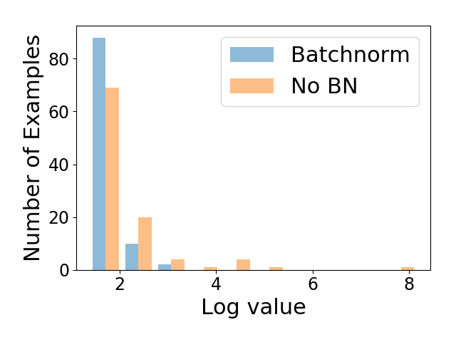
Figure 1: Let h1,h2,h3h_{1},h_{2},h_{3} denote the 1st, 2nd, and 3rd blocks of a 16-layer WideResNet and JiJ_{i} the Jacobian of the output w.r.t layer ii. In log-scale we plot a histogram of the 100 largest values on the training set of ∑i=13‖hi‖​‖Ji‖/γ\sum_{i=1}^{3}\|h_{i}\|\|J_{i}\|/\gamma for a WideResNet trained with and without Batchnorm on CIFAR10, where γ\gamma is the example’s margin.

In Figure 1, we plot the distribution over the sum of products of Jacobian and hidden layer norms (which is the leading term of the bound in our full Theorem 7.1) for a WideResNet (Zagoruyko and Komodakis 2016) trained with and without Batchnorm. Figure 1 shows that this sum blows up for networks trained without Batchnorm, indicating that the terms in our bound are empirically relevant for explaining data-dependent regularization.

An immediate bottleneck in proving Theorem 1.1 is that standard tools require fixing the hypothesis class before looking at training data, whereas conditioning on data-dependent properties makes the hypothesis class a random object depending on the data. A natural attempt is to augment the loss with indicators on the intended data-dependent quantities {γi}\{\gamma_{i}\}, with desired bounds {κi}\{\kappa_{i}\} as follows:

laug=(lold−1)​∏properties ​γi𝟙​(γi≤κi)+1\displaystyle l_{\textup{aug}}=(l_{\textup{old}}-1)\prod_{\textup{properties }\gamma_{i}}\mathbbm{1}(\gamma_{i}\leq\kappa_{i})+1

This augmented loss upper bounds the original loss lold∈[0,1]l_{\textup{old}}\in[0,1], with equality when all properties hold for the training data. The augmentation lets us reason about a hypothesis class that is independent of the data by directly conditioning on data-dependent properties in the loss. The main challenges with this approach are twofold: 1) designing the correct set of properties and 2) proving generalization of the final loss laugl_{\textup{aug}}, a complicated function of the network.

Our main tool is covering numbers: Lemma 4.1 shows that a composition of functions (i.e, a neural network) has low covering number if the output is worst-case Lipschitz at each level of the composition and internal layers are bounded in norm. Unfortunately, the standard neural net loss satisfies neither of these properties (without exponential dependencies on depth). However, by augmenting with properties γ\gamma, we can guarantee they hold. One technical challenge is that augmenting the loss makes it harder to reason about covering, as the indicators can introduce complicated dependencies between layers.

Our main technical contributions are: 1) We demonstrate how to augment a composition of functions to make it Lipschitz at all layers, and thus easy to cover. Before this augmentation, the Lipschitz constant could scale exponentially in depth (Theorem 4.4). 2) We reduce covering a complicated sequence of operations to covering the individual operations (Theorem 4.3). 3) By combining 1 and 2, it follows cleanly that our augmented loss on neural networks has low covering number and therefore has good generalization. Our bound scales polynomially, not exponentially, in the depth of the network when the network has good Lipschitz constants on the training data (Theorem 7.1).

As a complement to the main theoretical results in this paper, we show empirically in Section 8 that directly regularizing our complexity measure can result in improved test performance.

2 Related Work

Zhang et al. 2016 and Neyshabur et al. 2017b show that generalizaton in deep learning often disobeys conventional statistical wisdom. One of the approaches adopted torwards explaining generalization is implicit regularization; numerous recent works have shown that the training method prefers minimum norm or maximum margin solutions (Soudry et al. 2018; Li et al. 2018b; Ji and Telgarsky 2018; Gunasekar et al. 2017; Gunasekar et al. 2018a; Gunasekar et al. 2018b; Wei et al. 2018). With the exception of (Wei et al. 2018), these papers analyze simplified settings and do not apply to larger neural networks.

This paper more closely follows a line of work related to Rademacher complexity bounds for neural networks (Neyshabur et al. 2015b; Neyshabur et al. 2018; Bartlett et al. 2017; Golowich et al. 2017; Li et al. 2018a). For a comparison, see the introduction. There has also been work on deriving PAC-Bayesian bounds for generalization (Neyshabur et al. 2017b; Neyshabur et al. 2017a; Nagarajan and Kolter 2019). Dziugaite and Roy 2017a optimize a bound to compute non-vacuous bounds for generalization error. Another line of work analyzes neural nets via their behavior on noisy inputs. Neyshabur et al. 2017b prove PAC-Bayesian generalization bounds for random networks under assumptions on the network’s empirical noise stability. Arora et al. 2018 develop a notion of noise stability that allows for compression of a network under an appropriate noise distribution. They additionally prove that the compressed network generalizes well. In comparison, our Lipschitzness construction also relates to noise stability, but our bounds hold for the original network and do not rely on the particular noise distribution.

Nagarajan and Kolter 2019 use PAC-Bayes bounds to prove a similar result as ours for generalization of a network with bounded hidden layer and Jacobian norms. The main difference is that their bounds depend on the inverse relu preactivations, which are found to be large in practice (Nagarajan and Kolter 2019); our bounds apply to smooth activations and avoid this dependence at the cost of an additional factor in the Jacobian norm (shown to be empirically small). We note that the choice of smooth activations is empirically justified (Clevert et al. 2015; Klambauer et al. 2017). We also work with Rademacher complexity and covering numbers instead of the PAC-Bayes framework. It is relatively simple to adapt our techniques to relu networks to produce a similar result to that of Nagarajan and Kolter 2019, by conditioning on large pre-activation values in our Lipschitz augmentation step (see Section 4.2). In Section F, we provide a sketch of this argument and obtain a bound for relu networks that is polynomial in hidden layer and Jacobian norms and inverse preactivations. However, it is not obvious how to adapt the argument of Nagarajan and Kolter 2019 to activation functions whose derivatives are not piecewise-constant.

Dziugaite and Roy 2018; Dziugaite and Roy 2017b develop PAC-Bayes bounds for data-dependent priors obtained via some differentially private mechanism. Their bounds are for a randomized classifier sampled from the prior, whereas we analyze a deterministic, fixed model.

Novak et al. 2018 empirically demonstrate that the sensitivity of a neural net to input noise correlates with generalization. Sokolić et al. 2017; Krueger and Memisevic 2015 propose stability-based regularizers for neural nets. Hardt et al. 2015 show that models which train faster tend to generalize better. Keskar et al. 2016; Hoffer et al. 2017 study the effect of batch size on generalization. Brutzkus et al. 2017 analyze a neural network trained on hinge loss and linearly separable data and show that gradient descent recovers the exact separating hyperplane.

3 Notation

Let 𝟙​(E)\mathbbm{1}(E) be the indicator function of event EE. Let l0-1l_{\textup{0-1}} denote the standard 0-1 loss. For κ≥0\kappa\geq 0, Let 𝟙≤κ​(⋅)\mathbbm{1}_{\leq\kappa}(\cdot) be the softened indicator function defined as

𝟙≤κ​(t)={1 if ​t≤κ2−t/κ if ​κ≤t≤2​κ0 if ​2​κ≤t\displaystyle\mathbbm{1}_{\leq\kappa}(t)=\left\{\begin{array}[]{ll}1&\textup{ if }t\leq\kappa\\ 2-t/\kappa&\textup{ if }\kappa\leq t\leq 2\kappa\\ 0&\textup{ if }2\kappa\leq t\\ \end{array}\right.

Note that 𝟙≤κ\mathbbm{1}_{\leq\kappa} is κ−1\kappa^{-1}-Lipschitz. Define the norm ∥⋅∥p,q\|\cdot\|_{p,q} by ‖A‖p,q≜(∑j(∑iAi,jp)q/p)1/q\|A\|_{p,q}\triangleq\Big(\sum_{j}\big(\sum_{i}A_{i,j}^{p}\big)^{q/p}\Big)^{1/q}. Let PnP_{n} be a uniform distribution over nn points {x1,…,xn}⊂𝒟x\{x_{1},\dots,x_{n}\}\subset\mathcal{D}_{x}. Let ff be a function that maps 𝒟x\mathcal{D}_{x} to some output space 𝒟f\mathcal{D}_{f}, and assume both spaces are equipped with some norms |||⋅|||{|\kern-1.07639pt|\kern-1.07639pt|\cdot|\kern-1.07639pt|\kern-1.07639pt|} (these norms can be different but we use the same notations for them). Then the L2(Pn,|||⋅|||)L_{2}(P_{n},{|\kern-1.07639pt|\kern-1.07639pt|\cdot|\kern-1.07639pt|\kern-1.07639pt|}) norm of the function ff is defined as

∥f∥L2(Pn,|||⋅|||)≜(1n∑i|||f(xi)|||2)1/2\|f\|_{L_{2}(P_{n},{|\kern-0.75346pt|\kern-0.75346pt|\cdot|\kern-0.75346pt|\kern-0.75346pt|})}\triangleq\left(\frac{1}{n}\sum_{i}{|\kern-1.07639pt|\kern-1.07639pt|f(x_{i})|\kern-1.07639pt|\kern-1.07639pt|}^{2}\right)^{1/2}

We use DD to denote total derivative operator, and thus D​f​(x)Df(x) represents the Jacobian of ff at xx. Suppose ℱ\mathcal{F} is a family of functions from 𝒟x\mathcal{D}_{x} to 𝒟f\mathcal{D}_{f}. Let 𝒞⁡(ϵ,ℱ,ρ)\mathcal{C}(\epsilon,\mathcal{F},\rho) be the covering number of the function class ℱ\mathcal{F} w.r.t. metric ρ\rho with cover size ϵ\epsilon. In many cases, the covering number depends on the examples through the norms of the examples, and in this paper we only work with these cases. Thus, we let 𝒩⁡(ϵ,ℱ,s)\mathcal{N}(\epsilon,\mathcal{F},s) be the maximum covering number for any possible nn data points with norm not larger than ss. Precisely, if we define 𝒫n,s\mathcal{P}_{n,s} to be the set of all possible uniform distributions supported on nn data points with norms not larger than ss, then

𝒩(ϵ,ℱ,s)≜supPn∈𝒫n,s𝒞(ϵ,ℱ,L2(Pn,|||⋅|||))\mathcal{N}(\epsilon,\mathcal{F},s)\triangleq\sup_{P_{n}\in\mathcal{P}_{n,s}}\mathcal{C}(\epsilon,\mathcal{F},L_{2}(P_{n},{|\kern-1.07639pt|\kern-1.07639pt|\cdot|\kern-1.07639pt|\kern-1.07639pt|}))

Suppose ℱ\mathcal{F} contains functions with mm inputs that map from a tensor product mm Euclidean space to Euclidean space, then we define

𝒩(ϵ,ℱ,(s1,…,sm))≜supP:∀(x1,…,xm)∈supp​(P)‖xi‖≤si𝒞(ϵ,ℱ,L2(P))\mathcal{N}(\epsilon,\mathcal{F},(s_{1},\dots,s_{m}))\triangleq\sup_{\begin{subarray}{c}P:\forall(x_{1},\dots,x_{m})\in\text{supp}(P)\\ \|x_{i}\|\leq s_{i}\end{subarray}}\mathcal{C}(\epsilon,\mathcal{F},L_{2}(P))

4 Overview of Main Results and Proof Techniques

In this section, we give a general overview of the main technical results and outline how to prove them with minimal notation. We will point to later sections where many statements are formalized.

To simplify the core mathematical reasoning, we abstract feed-forward neural networks (including residual networks) as compositions of operations. Let ℱ1,…,ℱk\mathcal{F}_{1},\dots,\mathcal{F}_{k} be a sequence of families of functions (corresponding to families of single layer neural nets in the deep learning setting) and ℓ\ell be a Lipschitz loss function taking values in [0,1][0,1]. We study the compositions of ℓ\ell and functions in ℱi\mathcal{F}_{i}’s:

ℒ≜ℓ∘ℱk∘ℱk−1⋯∘ℱ1={ℓ∘fk∘fk−1∘⋯∘f1:∀i,fi∈ℱi}\displaystyle\mathcal{L}\triangleq\ell\circ\mathcal{F}_{k}\circ\mathcal{F}_{k-1}\cdots\circ\mathcal{F}_{1}=\{\ell\circ f_{k}\circ f_{k-1}\circ\cdots\circ f_{1}:\forall i,f_{i}\in\mathcal{F}_{i}\} (4)

Textbook results (Bartlett and Mendelson 2002) bound the generalization error by the Rademacher complexity (formally defined in Section A) of the family of losses ℒ\mathcal{L}, which in turn is bounded by the covering number of ℒ\mathcal{L} through Dudley’s entropy integral theorem (Dudley 1967). Modulo minor nuances, the key remaining question is to give a tight covering number bound for the family ℒ\mathcal{L} for every target cover size ϵ\epsilon in a certain range (often, considering ϵ∈[1/nO⁡(1),1]\epsilon\in[1/n^{O(1)},1] suffices).

As alluded to in the introduction, generalization error bounds obtained through this machinery only depend on the (training) data through the margin in the loss function, and our aim is to utilize more data-dependent properties. Towards understanding which data-dependent properties are useful to regularize, it is helpful to revisit the data-independent covering technique of (Bartlett et al. 2017), the skeleton of which is summarized below.

Recall that 𝒩⁡(ϵ,ℱ,s)\mathcal{N}(\epsilon,\mathcal{F},s) denotes the covering number for arbitrary nn data points with norm less than ss. The following lemma says that if the intermediate variable (or the hidden layer) fi∘⋯∘f1(x)f_{i}\circ\cdots\circ f_{1}(x) is bounded, and the composition of the rest of the functions l∘fk∘⋯∘fi+1(x)l\circ f_{k}\circ\cdots\circ f_{i+1}(x) is Lipschitz, then small covering number of local functions imply small covering number for the composition of functions.

Lemma 4.1.

[abstraction of techniques in (Bartlett et al. 2017)] In the context above, assume:

  • 1.

    for any x∈supp​(Pn)x\in\text{supp}(P_{n}), |||fi∘⋯∘f1(x)|||≤si{|\kern-1.07639pt|\kern-1.07639pt|f_{i}\circ\cdots\circ f_{1}(x)|\kern-1.07639pt|\kern-1.07639pt|}\leq s_{i}.

  • 2.

    ℓ∘fk∘⋯∘fi+1\ell\circ f_{k}\circ\cdots\circ f_{i+1} is κi\kappa_{i}-Lipschitz for all ii.

Then, we have the following covering number bound for ℒ\mathcal{L} (for any choice of ϵ1,…,ϵk>0\epsilon_{1},\dots,\epsilon_{k}>0):

log⁡𝒩⁡(∑i=1kκi​ϵi,ℒ,s0)≤∑i=1klog⁡𝒩⁡(ϵi,ℱi,si−1)\log\mathcal{N}(\sum_{i=1}^{k}\kappa_{i}\epsilon_{i},\mathcal{L},s_{0})\leq\sum_{i=1}^{k}\log\mathcal{N}(\epsilon_{i},\mathcal{F}_{i},s_{i-1})

The lemma says that the log covering number and the cover size scale linearly if the Lipschitzness parameters and norms remain constant. However, these two quantities, in the worst case, can easily scale exponentially in the number of layers, and they are the main sources of the dependency of product of spectral/Frobenius norms of layers in (Golowich et al. 2017; Bartlett et al. 2017; Neyshabur et al. 2017a; Neyshabur et al. 2015b) More precisely, the worst-case Lipschitzness over all possible data points can be exponentially bigger than the average/typical Lipschitzness for examples randomly drawn from the training or test distribution. We aim to bridge this gap by deriving a generalization error bound that only depends on the Lipschitzness and boundedness on the training examples.

Our general approach, partially inspired by margin theory, is to augment the loss function by soft indicators of Lipschitzness and boundedness. Let hih_{i} be shorthand notation for fi∘⋯∘f1f_{i}\circ\cdots\circ f_{1}, the ii-th intermediate value, and let z⁡(x)≜ℓ⁡(hk​(x))z(x)\triangleq\ell(h_{k}(x)) be the original loss. Our first attempt considered:

z~′​(x)≜1+(z⁡(x)−1)⋅∏i=1k𝟙≤si​(‖hi​(x)‖)⋅∏i=1k𝟙≤κi​(‖∂z/∂hi‖op)\displaystyle\tilde{z}^{\prime}(x)\triangleq 1+(z(x)-1)\cdot\prod_{i=1}^{k}\mathbbm{1}_{\leq s_{i}}(\|h_{i}(x)\|)\cdot\prod_{i=1}^{k}\mathbbm{1}_{\leq\kappa_{i}}(\left\|{\partial z}/{\partial h_{i}}\right\|_{\textup{op}}) (5)

Since zz takes values in [0,1][0,1], the augmented loss z~′\tilde{z}^{\prime} is an upper bound on the original loss zz with equality when all the indicators are satisfied with value 11. The hope was that the indicators would flatten those regions where hih_{i} is not bounded and where zz is not Lipschitz in hih_{i}. However, there are two immediate issues. First, the soft indicators functions are themselves functions of hih_{i}. It’s unclear whether the augmented function can be Lipschitz with a small constant w.r.t hih_{i}, and thus we cannot apply Lemma 4.1.11 1 A priori, it’s also unclear what “Lipschitz in hih_{i}” means since the z¯′\bar{z}^{\prime} does not only depend on xx through hih_{i}. We will formalize this in later section after defining proper language about dependencies between variables. Second, the augmented loss function becomes complicated and doesn’t fall into the sequential computation form of Lemma 4.1, and therefore even if Lipschitzness is not an issue, we need new covering techniques beyond Lemma 4.1.

We address the first issue by recursively augmenting the loss function by multiplying more soft indicators that bound the Jacobian of the current function. The final loss z~\tilde{z} reads:22 2 Unlike in equation (5), we don’t augment the Jacobian of the loss w.r.t the layers. This allows us to deal with non-differentiable loss functions such as ramp loss.

z~(x)≜1+(z(x)−1)⋅∏i=1k𝟙≤si(∥hi(x)∥)⋅∏1≤i≤j≤k𝟙≤κj←i(∥Dfj∘⋯∘fi[hi−1]∥op)\displaystyle\tilde{z}(x)\triangleq 1+(z(x)-1)\cdot\prod_{i=1}^{k}\mathbbm{1}_{\leq s_{i}}(\|h_{i}(x)\|)\cdot\prod_{1\leq i\leq j\leq k}\mathbbm{1}_{\leq\kappa_{j\leftarrow i}}(\|Df_{j}\circ\cdots\circ f_{i}[h_{i-1}]\|_{\textup{op}}) (6)

where κj←i\kappa_{j\leftarrow i}’s are user-defined parameters. For our application to neural nets, we instantiate sis_{i} as the maximum norm of layer ii and κj←i\kappa_{j\leftarrow i} as the maximum norm of the Jacobian between layer jj and ii across the training dataset. A polynomial in κ,s\kappa,s can be shown to bound the worst-case Lipschitzness of the function w.r.t. the intermediate variables in the formula above.33 3 As mentioned in footnote 1, we will formalize the precise meaning of Lipschitzness later. By our choice of κ\kappa, ss, a) the training loss is unaffected by the augmentation and b) the worst-case Lipschitzness of the loss is controlled by a polynomial of the Lipschitzness on the training examples. We provide an informal overview of our augmentation procedure in Section 4.2 and formally state definitions and guarantees in Section 6. The downside of the Lipschitz augmentation is that it further complicates the loss function. Towards covering the loss function (assuming Lipschitz properties) efficiently, we extend Lemma 4.1, which works for sequential compositions of functions, to general families of formulas, or computational graphs. We informally overview this extension in Section 4.1 using a minimal set of notations, and in Section 5, we give a formal presentation of these results.

Combining the Lipschitz augmentation and graphs covering results, we obtain a covering number bound of augmented loss. The theorem below is formally stated in Theorem 6.3 of Section 6.

Theorem 4.2.

Let ℒ~\tilde{\mathcal{L}} be the family of augmented losses defined in (6). For cover resolutions ϵi\epsilon_{i} and values κ~i\tilde{\kappa}_{i} that are polynomial in the parameters si,κj←is_{i},\kappa_{j\leftarrow i}, we obtain the following covering number bound for ℒ~\tilde{\mathcal{L}}:

log⁡𝒩⁡(∑iϵi​κ~i,ℒ~,s0)≤∑ilog⁡𝒩⁡(ϵi,ℱi,si−1)+∑ilog⁡𝒩⁡(ϵi,D​ℱi,si−1)\displaystyle\log\mathcal{N}(\sum_{i}\epsilon_{i}\tilde{\kappa}_{i},\tilde{\mathcal{L}},s_{0})\leq\sum_{i}\log\mathcal{N}(\epsilon_{i},\mathcal{F}_{i},s_{i-1})+\sum_{i}\log\mathcal{N}(\epsilon_{i},D\mathcal{F}_{i},s_{i-1})

where D​ℱiD\mathcal{F}_{i} denotes the function class obtained from applying the total derivative operator to all functions in ℱi\mathcal{F}_{i}.

Now, following the standard technique of bounding Rademacher complexity via covering numbers, we can obtain generalization error bounds for augmented loss. For the demonstration of our technique, suppose that the following simplification holds:

log⁡𝒩⁡(ϵi,D​ℱi,si−1)=log⁡𝒩⁡(ϵi,ℱi,si−1)=si−12/ϵi2\log\mathcal{N}(\epsilon_{i},D\mathcal{F}_{i},s_{i-1})=\log\mathcal{N}(\epsilon_{i},\mathcal{F}_{i},s_{i-1})=s_{i-1}^{2}/\epsilon_{i}^{2}

Then after minimizing the covering number bound in ϵi\epsilon_{i} via standard techniques, we obtain the below generalization error bound on the original loss for parameters κ~i\tilde{\kappa}_{i} alluded to in Theorem 4.2 and formally defined in Theorem 6.2. When the training examples satisfy the augmented indicators, 𝔼train[z~]=𝔼train[z]\mathop{\mathbb{E}}\displaylimits_{\textup{train}}[\tilde{z}]=\mathop{\mathbb{E}}\displaylimits_{\textup{train}}[z], and because z~\tilde{z} bounds zz from above, we have

𝔼test[z]−𝔼train[z]≤𝔼test[z~]−𝔼train[z~]≤O~​((∑iκ~i2/3​si−12/3)3/2n+log⁡(1/δ)n)\displaystyle\mathop{\mathbb{E}}\displaylimits_{\textup{test}}\left[z\right]-\mathop{\mathbb{E}}\displaylimits_{\textup{train}}\left[z\right]\leq\mathop{\mathbb{E}}\displaylimits_{\textup{test}}\left[\tilde{z}\right]-\mathop{\mathbb{E}}\displaylimits_{\textup{train}}\left[\tilde{z}\right]\leq\widetilde{O}\Bigg(\frac{\left(\sum_{i}\tilde{\kappa}_{i}^{2/3}s_{i-1}^{2/3}\right)^{3/2}}{\sqrt{n}}+\sqrt{\frac{\log(1/\delta)}{n}}\Bigg) (7)

4.1 Overview of Computational Graph Covering

To obtain the augmented z~\tilde{z} defined in (6), we needed to condition on data-dependent properties which introduced dependencies between the various layers. Because of this, Lemma 4.1 is no longer sufficient to cover z~\tilde{z}. In this section, we informally overview how to extend Lemma 4.1 to cover more general functions via the notion of computational graphs. Section 5 provides a more formal discussion.

A computational graph G⁡(𝒱,ℰ,{RV})G(\mathcal{V},\mathcal{E},\{R_{V}\}) is an acyclic directed graph with three components: the set of nodes 𝒱\mathcal{V} corresponds to variables, the set of edges ℰ\mathcal{E} describes dependencies between these variables, and {RV}\{R_{V}\} contains a list of composition rules indexed by the variables VV’s, representing the process of computing VV from its direct predecessors. For simplicity, we assume the graph contains a unique sink, denoted by OGO_{G}, and we call it the “output node”. We also overload the notation OGO_{G} to denote the function that the computational graph GG finally computes. Let ℐG={I1,…,Ip}\mathcal{I}_{G}=\{I_{1},\dots,I_{p}\} be the subset of nodes with no predecessors, which we call the “input nodes” of the graph.

The notion of a family of computational graphs generalizes the sequential family of function compositions in (4). Let 𝒢={G⁡(𝒱,ℰ,{RV})}\mathcal{G}=\{G(\mathcal{V},\mathcal{E},\{R_{V}\})\} be a family of computational graphs with shared nodes, edges, output node, and input nodes (denoted by ℐ\mathcal{I}). Let ℜV\mathfrak{R}_{V} be the collection of all possible composition rules used for node VV by the graphs in the family 𝒢\mathcal{G}. This family 𝒢\mathcal{G} defines a set of functions O𝒢≜{OG:G∈𝒢}O_{\mathcal{G}}\triangleq\{O_{G}:G\in\mathcal{G}\}.

The theorem below extends Lemma 4.1. In the computational graph interpretation, Lemma 4.1 applies to a sequential family of computational graphs with kk internal nodes V1,…,VkV_{1},\ldots,V_{k}, where each ViV_{i} computes the function fif_{i}, and the output computes the composition OG=ℓ∘fk∘⋯∘f1=zO_{G}=\ell\circ f_{k}\cdots\circ f_{1}=z. However, the augmented loss z~\tilde{z} no longer has this sequential structure, requiring the below theorem for covering generic families of computational graphs. We show that covering a general family of computational graphs can be reduced to covering all the local composition rules.

Theorem 4.3 (Informal and weaker version of Theorem 5.3).

Suppose that there is an ordering (V1,…,Vm)(V_{1},\dots,V_{m}) of the nodes, so that after cutting out nodes V1,…,Vi−1V_{1},\dots,V_{i-1}, the node ViV_{i} becomes a leaf node and the output OGO_{G} is κVi\kappa_{V_{i}}-Lipschitz w.r.t to ViV_{i} for all G∈𝒢G\in\mathcal{G}. In addition, assume that for all G∈𝒢G\in\mathcal{G}, the node VV’s value has norm at most sVs_{V}. Let pr​(V)\textup{pr}(V) be all the predecessors of VV and spr​(V)s_{\textup{pr}(V)} be the list of norm upper bounds of the predecessors of VV.

Then, small covering numbers for all of the local composition rules of VV with resolution ϵV\epsilon_{V} would imply small covering number for the family of computational graphs with resolution ∑VϵV​κV\sum_{V}\epsilon_{V}\kappa_{V}:

log⁡𝒩⁡(∑V∈𝒱∖ℐ∪{O}κV​ϵV+ϵO,O𝒢,sℐ)≤∑V∈𝒱∖ℐlog⁡𝒩⁡(ϵV,ℜV,spr​(V))\displaystyle\log\mathcal{N}(\sum_{V\in\mathcal{V}\setminus\mathcal{I}\cup\{O\}}\kappa_{V}\epsilon_{V}+\epsilon_{O},O_{\mathcal{G}},s_{\mathcal{I}})\leq\sum_{V\in\mathcal{V}\setminus\mathcal{I}}\log\mathcal{N}(\epsilon_{V},\mathfrak{R}_{V},s_{\textup{pr}(V)}) (8)

In Section 5 we formalize the notion of “cutting” nodes from the graph. The condition that node VV’s value has norm at most sVs_{V} is a simplification made for expositional purposes; our full Theorem 5.3 also applies if OGO_{G} collapses to a constant whenever node VV’s value has norm greater than sVs_{V}. This allows for the softened indicators 𝟙≤si​(‖hi​(x)‖)\mathbbm{1}_{\leq s_{i}}(\|h_{i}(x)\|) used in (6).

4.2 Lipschitz Augmentation of Computational Graphs

The covering number bound of Theorem 4.3 relies on Lipschitzness w.r.t internal nodes of the graph under a worst-case choice of inputs. For deep networks, this can scale exponentially in depth via the product of weight norms and easily be larger than the average Lipschitz-ness over typical inputs. In this section, we explain a general operation to augment sequential graphs (such as neural nets) into graphs with better worst-case Lipschitz constants, so tools such as Theorem 4.3 can be applied. Formal definitions and theorem statements are in Section 6.

The augmentation relies on introducing terms such as the soft indicators in equation (5) and (6) which condition on data-dependent properties. As outlined in Section 4, they will translate to the data-dependent properties in the generalization bounds. We also require the augmented function to upper bound the original.

We will present a generic approach to augment function compositions such as z≜ℓ∘fk∘…∘f1z\triangleq\ell\circ f_{k}\circ\ldots\circ f_{1}, whose Lipschitz constants are potentially exponential in depth, with only properties involving the norms of the inter-layer Jacobians. We will produce z~\tilde{z}, whose worst-case Lipschitzness w.r.t. internal nodes can be polynomial in depth.

Informal explanation of Lipschitz augmentation: In the same setting of Section 4, recall that in (5), our first unsuccessful attempt to smooth out the function was by multiplying indicators on the norms of the derivatives of the output: ∏i=1k𝟙≤κi​(‖∂z/∂hi‖op)\prod_{i=1}^{k}\mathbbm{1}_{\leq\kappa_{i}}(\left\|{\partial z}/{\partial h_{i}}\right\|_{\textup{op}}). The difficulty lies in controlling the Lipschitzness of the new terms ‖∂z/∂hi‖op\|\partial z/\partial h_{i}\|_{\textup{op}} that we introduce: by the chain rule, we have the expansion ∂z∂hi=∂z∂hk∂hk∂hk−1⋯∂hi+1∂hi\frac{\partial z}{\partial h_{i}}=\frac{\partial{z}}{\partial h_{k}}\frac{\partial h_{k}}{\partial h_{k-1}}\cdots\frac{\partial h_{i+1}}{\partial h_{i}}, where each hj′h_{j^{\prime}} is itself a function of hjh_{j} for j′>jj^{\prime}>j. This means ∂z∂hi\frac{\partial z}{\partial h_{i}} is a complicated function in the intermediate variables hjh_{j} for 1≤j≤k1\leq j\leq k. Bounding the Lipschitzness of ∂z∂hi\frac{\partial z}{\partial h_{i}} requires accounting for the Lipschitzness of every term in its expansion, which is challenging and creates complicated dependencies between variables.

Our key insight is that by considering a more complicated augmentation which conditions on the derivatives between all intermediate variables, we can still control Lipschitzness of the system, leading to the more involved augmentation presented in (6). Our main technical contribution is Theorem 4.4, which we informally state below.

Theorem 4.4 (Informal version of Theorem 6.2).

The functions z~\tilde{z} (defined in (6)) can be computed by a family of computational graphs 𝒢~\widetilde{\mathcal{G}} illustrated in Figure 2. This family has internal nodes ViV_{i} and JiJ_{i} computing hih_{i} and D​fi​[hi−1]Df_{i}[h_{i-1}], respectively, and computes a modified output rule that augments the original with soft indicators. These soft indicators condition that the norms of the Jacobians and hih_{i} are bounded by parameters κj←i,si\kappa_{j\leftarrow i},s_{i}.

Importantly, the output OG~O_{\tilde{G}} is κ~Vi\tilde{\kappa}_{V_{i}}, κ~Ji\tilde{\kappa}_{J_{i}}-Lipschitz w.r.t. ViV_{i}, JiJ_{i}, respectively, after cutting nodes V1,J1,…,Vi−1,Ji−1V_{1},J_{1},\ldots,V_{i-1},J_{i-1}, for parameters κ~Vi\tilde{\kappa}_{V_{i}}, κ~Ji\tilde{\kappa}_{J_{i}} that are polynomials in κj←i\kappa_{j\leftarrow i}, sis_{i}.

In addition, the augmented function z~\tilde{z} will upper bound the original with equality when all the indicators are satisfied. The crux of the proof is leveraging the chain rule to decompose ∂z∂hi\frac{\partial z}{\partial h_{i}} into a product and then applying a telescoping argument to bound the difference in the product by differences in individual terms. In Section 6 we present a formal version of this result and also apply Theorem 4.3 to produce a covering number bound for 𝒢~\widetilde{\mathcal{G}}.

Figure 2: Lipschitz augmentation (informally defined).
Refer to caption

5 Covering of Computational Graphs

This section is a formal version of Section 4.1 with full definition and theorem statements. In this section, we adapt the notion of a computational graph to our setting. In Section 5.1, we formalize the notion of a computational graph and demonstrate how neural networks fit under this framework. In Section 5.2, we define the notion of release-Lipschitzness that abstracts the sequential notion of Lipschitzness in Lemma 4.1. We show that when this release-Lipschitzness condition and a boundedness condition on the internal nodes hold, it is possible to cover a family of computational graphs by simply covering the function class at each vertex.

5.1 Formalization of computational graphs

When we augment the neural network loss with data-dependent properties, we introduce dependencies between the various layers, making it complicated to cover the augmented loss. We use the notion of computational graphs to abstractly model these dependencies.

Computational graphs are originally introduced by Bauer 1974 to represent computational processes and study error propagation. Recall the notation G⁡(𝒱,ℰ,{RV})G(\mathcal{V},\mathcal{E},\{R_{V}\}) introduced for a computational graph in Section 4.1, with input nodes ℐG={I1,…,Ip}\mathcal{I}_{G}=\{I_{1},\dots,I_{p}\} and output node denoted by OGO_{G}. (It’s straightforward to generalize to scenarios with multiple output nodes.)

For every variable V∈𝒱V\in\mathcal{V}, let 𝒟V\mathcal{D}_{V} be the space that VV resides in. If VV has tt direct predecessors C1,…,CtC_{1},\dots,C_{t}, then the associated composition rule RVR_{V} is a function that maps 𝒟C1⊗⋯⊗𝒟Ct\mathcal{D}_{C_{1}}\otimes\cdots\otimes\mathcal{D}_{C_{t}} to 𝒟V\mathcal{D}_{V}. If VV is an input node, then the composition rule RVR_{V} is not relevant. For any node VV, the computational graph defines/induces a function that computes the variable VV from inputs, or in mathematical words, that maps the inputs space 𝒟I1⊗⋯⊗𝒟Ip\mathcal{D}_{I_{1}}\otimes\cdots\otimes\mathcal{D}_{I_{p}} to 𝒟V\mathcal{D}_{V}. This associated function, denoted by VV again with slight abuse of notations, is defined recursively as follows: set V⁡(x1,…,xp)V(x_{1},\dots,x_{p}) to

{xiif V is the i-th input node IiRV​(C1​(x1,…,xp),…,Ct​(x1,…,xp))if V has t direct predecessors C1,…,Ct\displaystyle\left\{\begin{array}[]{ll}x_{i}&\textup{if $V$ is the $i$-th input node $I_{i}$}\\ R_{V}(C_{1}(x_{1},\dots,x_{p}),\dots,C_{t}(x_{1},\dots,x_{p}))&\textup{if $V$ has $t$ direct predecessors $C_{1},\dots,C_{t}$}\end{array}\right.

More succinctly, we can write V=RV∘(C1⊗⋯⊗Ct)V=R_{V}\circ(C_{1}\otimes\cdots\otimes C_{t}). We also overload the notation OGO_{G} to denote the function that the computational graph GG finally computes (which maps 𝒟I1⊗⋯⊗𝒟Ip\mathcal{D}_{I_{1}}\otimes\cdots\otimes\mathcal{D}_{I_{p}} to 𝒟O\mathcal{D}_{O}). For any set 𝒮={V1,…,Vt}⊆𝒱\mathcal{S}=\{V_{1},\ldots,V_{t}\}\subseteq\mathcal{V}, use 𝒟𝒮\mathcal{D}_{\mathcal{S}} to denote the space 𝒟V1⊗⋯⊗𝒟Vt\mathcal{D}_{V_{1}}\otimes\cdots\otimes\mathcal{D}_{V_{t}}. We use pr​(G,V)\textup{pr}(G,V) to denote the set of direct predecessors of VV in graph GG, or simply pr​(V)\textup{pr}(V) when the graph GG is clear from context.

Example 5.1 (Feed-forward neural networks).

For an activation function ϕ\phi and parameters {W(i)}\{W^{(i)}\} we compute a neural net F:ℝdI→ℝdOF:\mathbb{R}^{d_{I}}\to\mathbb{R}^{d_{O}} as follows: F(x)=W(r)ϕ(⋯ϕ(W(1)x)⋯)F(x)=W^{(r)}\phi(\cdots\phi(W^{(1)}x)\cdots). Figure 3 depicts how this neural network fits into a computational graph with one input node, 2​r−12r-1 internal nodes, and a single output. Here we treat matrix operations and activations as distinct layers, and map each layer to a node in the computational graph.

Refer to caption
Figure 3: The computational graph corresponding to a neural network with rr weight matrices. Odd-indexed layers multiply matrices and even-indexed layers apply the activation ϕ\phi.

5.2 Reducing graph covering to local function covering

In this section we introduce the notion of a family of computational graphs, generalizing the sequential family of function compositions in (4). We define release-Lipschitzness, a condition which allows reduce covering the entire the graph family to covering the composition rules at each node. We formally state this reduction in Theorem 5.3.

Family of computational graphs:

Let 𝒢={G⁡(𝒱,ℰ,{RV}):{RV}∈ℜ}\mathcal{G}=\{G(\mathcal{V},\mathcal{E},\{R_{V}\}):\{R_{V}\}\in\mathfrak{R}\} be a family of computational graph with shared nodes and edges, where ℜ\mathfrak{R} is a collection of lists of composition rules. This family of computational graphs defines a set of functions O𝒢≜{OG:G∈𝒢}O_{\mathcal{G}}\triangleq\{O_{G}:G\in\mathcal{G}\}. We’d like to cover this set of functions in O𝒢O_{\mathcal{G}} with respect to some metric L(Pn,|||⋅|||)L(P_{n},{|\kern-1.07639pt|\kern-1.07639pt|\cdot|\kern-1.07639pt|\kern-1.07639pt|}).

For a list of composition rules {RV}∈ℜ\{R_{V}\}\in\mathfrak{R} and subset 𝒮⊆𝒱\mathcal{S}\subseteq\mathcal{V}, we define the projection of composition rules onto 𝒮\mathcal{S} by {RV}𝒮={RV:V∈𝒮}\{R_{V}\}_{\mathcal{S}}=\{R_{V}:V\in\mathcal{S}\}. Now let ℜS={{RV}𝒮:{RV}∈ℜ}\mathfrak{R}_{S}=\{\{R_{V}\}_{\mathcal{S}}:\{R_{V}\}\in\mathfrak{R}\} denote the marginal collection of the composition rules on node subset 𝒮\mathcal{S}.

For any computational graph GG and a non-input node V∈𝒱∖ℐV\in\mathcal{V}\setminus\mathcal{I}, we can define the following operation that “releases” VV from its dependencies on its predecessors by cutting all the inward edges: Let G\VG^{\backslash V} be sub-graph of GG where all the edges pointing towards VV are removed from the graph. Thus, by definition, VV becomes a new input node of the graph G\VG^{\backslash V}: ℐG\V={V}∪ℐG\mathcal{I}_{G^{\backslash V}}=\{V\}\cup\mathcal{I}_{G}. Moreover, we can “recover” the dependency by plugging the right value for VV in the new graph G\VG^{\backslash V}: Let V⁡(x)V(x) be the function associated to the node VV in graph GG, then we have

∀x∈𝒟ℐ,OG\V​(V⁡(x),x)=OG​(x)\displaystyle\forall x\in\mathcal{D}_{\mathcal{I}},\penalty\ \penalty\ O_{G^{\backslash V}}(V(x),x)=O_{G}(x) (11)

In our proofs, we will release variables in orders. Let 𝒮=(V1,…,Vm)\mathcal{S}=(V_{1},\dots,V_{m}) be an ordering of the intermediate variables 𝒱\(ℐ∪{O})\mathcal{V}\backslash(\mathcal{I}\cup\{O\}). We call 𝒮\mathcal{S} a forest ordering if for any ii, in the original graph GG, ViV_{i} at most depends on the input nodes and V1,…,Vi−1V_{1},\dots,V_{i-1}. For any sequence of variables (V1,…,Vt)(V_{1},\dots,V_{t}), we can define the graph obtained by releasing the variables in order: G\(V1,…,Vt)≜(⋯(G\V1)⋯)\VtG^{\backslash(V_{1},\dots,V_{t})}\triangleq(\cdots(G^{\backslash V_{1}})\cdots)^{\backslash V_{t}}. We next define the release-Lipschitz condition, which states that the graph function remains Lipschitz when we sequentially release vertices in a forest ordering of the graph.

Definition 5.2 (Release-Lipschitzness).

A graph GG is release-Lipschitz with parameters {κV}\{\kappa_{V}\} w.r.t a forest ordering of the internal nodes, denoted by (V1,…,Vm)(V_{1},\dots,V_{m}) if the following happens: upon releasing V1,…,VmV_{1},\dots,V_{m} in order from any G∈𝒢G\in\mathcal{G}, for any 0≤i≤m0\leq i\leq m, we have that the function defined by the released graph G\(V1,…,Vi)G^{\backslash(V_{1},\dots,V_{i})} is κVi\kappa_{V_{i}}-Lipschitz in the argument ViV_{i}, for any values of the rest of the input nodes (={V1,…,Vi−1}∪ℐG\{V_{1},\dots,V_{i-1}\}\cup\mathcal{I}_{G}.) We also say graph GG is release- Lipschitz if such a forest ordering exists.

Now we show that the release-Lipschitz condition allows us to cover any family of computational graphs whose output collapses when internal nodes are too large. The below is a formal and complete version of Theorem 4.3. For the augmented loss defined in (6), the function output collapses to 11 when internal computations are large. The proof is deferred to Section B.

Theorem 5.3.

Suppose 𝒢\mathcal{G} is a computational graph with the associated family of lists of composition rules ℜ\mathfrak{R}, as formally defined above. Let PnP_{n} be a uniform distribution over nn points in 𝒟ℐ\mathcal{D}_{\mathcal{I}}. Let κV\kappa_{V}, sVs_{V}, and ϵV\epsilon_{V} be three families of fixed parameters indexed by 𝒱\ℐ\mathcal{V}\backslash\mathcal{I} (whose meanings are defined below). Assume the following:

  • 1.

    Every G∈𝒢G\in\mathcal{G} is release-Lipschitz with parameters {κV}\{\kappa_{V}\} w.r.t a forest ordering of the internal nodes (V1,…,Vm)(V_{1},\dots,V_{m}) (the parameter κV\kappa_{V}’s and ordering doesn’t depend on the choice of GG.)

  • 2.

    For the same order as before, if (v,x)∈(𝒟V1⊗⋯⊗𝒟Vi)⊗𝒟ℐ(v,x)\in(\mathcal{D}_{V_{1}}\otimes\cdots\otimes\mathcal{D}_{V_{i}})\otimes\mathcal{D}_{\mathcal{I}} is an input of the released graph satisfying ‖|vj|‖≥sVj{|\kern-1.07639pt|\kern-1.07639pt|v_{j}|\kern-1.07639pt|\kern-1.07639pt|}\geq s_{V_{j}} for some j≤ij\leq i, then OG\(V1,…,Vi)​(v,x)=cO_{G^{\backslash(V_{1},\dots,V_{i})}}(v,x)=c for some constant cc.

Then, small covering numbers for all of the local composition rules of VV with resolution ϵV\epsilon_{V} would imply small covering number for the family of computational graphs with resolution ∑VϵV​κV\sum_{V}\epsilon_{V}\kappa_{V}:

log⁡𝒩⁡(∑V∈𝒱∖ℐ∪{O}κV​ϵV+ϵO,O𝒢,sℐ)≤∑V∈𝒱∖ℐlog⁡𝒩⁡(ϵV,ℜ{V},spr​(V))\displaystyle\log\mathcal{N}(\sum_{V\in\mathcal{V}\setminus\mathcal{I}\cup\{O\}}\kappa_{V}\epsilon_{V}+\epsilon_{O},O_{\mathcal{G}},s_{\mathcal{I}})\leq\sum_{V\in\mathcal{V}\setminus\mathcal{I}}\log\mathcal{N}(\epsilon_{V},\mathfrak{R}_{\{V\}},s_{\textup{pr}(V)}) (12)

6 Lipschitz Augmentation of Computational Graphs

In this section, we provide a more thorough and formal presentation of the augmentation framework of Section 4.2.

The covering number bound for the computational graph family 𝒢\mathcal{G} in Theorem 5.3 relies on the release-Lipschitzness condition (condition 1 of Theorem 5.3) and rarely holds for deep computational graphs such as deep neural networks. The conundrum is that the worst-case Lipschitzness as required in the release-Lipschitz condition44 4 We say the Lipschitzness required is worst case because the release-Lipschitz condition requires the Lipschitzness of nodes for any possible choice of inputs is very likely to scale in the product of the worst-case Lipschitzness of each operations in the graph, which can easily be exponentially larger than the average Lipschitzness over typical examples.

In this section, we first define a model of sequential computational graphs, which captures the class of neural networks. Before Lipschitz augmentation, the worst-case Lipschitz constant of graphs in this family could scale exponentially in the depth of the graph. In Definition 6.1, we generalize the operation of (6) to augment any family 𝒢\mathcal{G} of sequential graphs and produce a family 𝒢~\widetilde{\mathcal{G}} satisfying the release-Lipschitz condition. In Theorem 6.3, we combine this augmentation with the framework of 5.3 to produce general covering number bounds for the augmented graphs. For the rest of this section we will work with sequential families of computational graphs.

A sequential computational graph has nodes set 𝒱={I,V1,…,Vq,O}\mathcal{V}=\{I,V_{1},\ldots,V_{q},O\}, where II is the single input node, and all the edges are ℰ={(I,V1),(V1,V2),⋯,(Vq−1,Vq)}∪{(V1,O),…,(Vq,O)}\mathcal{E}=\{(I,V_{1}),(V_{1},V_{2}),\cdots,(V_{q-1},V_{q})\}\cup\{(V_{1},O),\dots,(V_{q},O)\}. We often use the notation V0V_{0} to refer to the input II. Below we formally define the augmentation operation.

Definition 6.1 (Lipschitz augmentation of sequential graphs).

Given a differentiable sequential computational graph GG with qq internal nodes V1,…,VqV_{1},\dots,V_{q}, define its Lipschitz augmentation G~\widetilde{G} as follows. We first add qq nodes to the graph denoted by J1,…,JqJ_{1},\dots,J_{q}. The composition rules for original internal nodes remain the same, and the composition rule for JiJ_{i} is defined as

R~Ji=D​RVi\displaystyle\widetilde{R}_{J_{i}}=DR_{V_{i}}

Here D​RViDR_{V_{i}} is the total derivative of the function RViR_{V_{i}}. In other words, the variable JiJ_{i} is a Jacobian for RViR_{V_{i}}, a linear operator that maps 𝒟Vi−1\mathcal{D}_{V_{i-1}} to 𝒟Vi\mathcal{D}_{V_{i}}. (Note that if ViV_{i}’s are considered as vector variables, then JiJ_{i}’s are matrix variables.) We equip the space of JiJ_{i} with operator norm, denoted by ∥⋅∥op\|\cdot\|_{\textup{op}}, induced by the original norms on spaces Vi−1V_{i-1} and ViV_{i}. The Lipschitz-ness w.r.t variable JiJ_{i} will be measured with operator norm.

We pre-determine a family of parameters κj←i\kappa_{j\leftarrow i} for all pairs (i,j)(i,j) with i≤ji\leq j. The final loss is augmented by a product of soft indicators that truncates the function when any of the Jacobians is much larger than κi←j\kappa_{i\leftarrow j} :

R~O(x,v1,…,vq,D1,…,Dq)≜(RO(x,v1,…,vq)−1)∏i≤j𝟙≤κj←i(∥Dj⋯Di∥op)+1\displaystyle\widetilde{R}_{O}(x,v_{1},\ldots,v_{q},D_{1},\ldots,D_{q})\triangleq(R_{O}(x,v_{1},\ldots,v_{q})-1)\prod_{i\leq j}\mathbbm{1}_{\leq\kappa_{j\leftarrow i}}(\|D_{j}\cdots D_{i}\|_{\textup{op}})+1

where x∈𝒟ℐx\in\mathcal{D}_{\mathcal{I}}, vi∈𝒟Viv_{i}\in\mathcal{D}_{V_{i}}, and Di∈𝒟JiD_{i}\in\mathcal{D}_{J_{i}}. Note that Dj⋯DiD_{j}\cdots D_{i} is the total derivative of VjV_{j} w.r.t ViV_{i}, and thus the κj←i\kappa_{j\leftarrow i} has the interpretation as an intended bound of the Jacobian between pairs of layers (variables). Figure 4 depicts the augmentation.

Note that under these definitions, we finally get that the output function of G~\widetilde{G} computes

OG~(x)=(OG(x)−1)∏i≤j𝟙≤κj←i(∥DVj(x)⋯DVi(x)∥op)+1\displaystyle O_{\widetilde{G}}(x)=(O_{G}(x)-1)\prod_{i\leq j}\mathbbm{1}_{\leq\kappa_{j\leftarrow i}}(\|DV_{j}(x)\cdots DV_{i}(x)\|_{\textup{op}})+1 (13)

which matches (6) for the example in Section 4. We note that the graph G~\tilde{G} contains the original GG as a subgraph. Furthermore, by Claim H.1, OG~O_{\tilde{G}} upper bounds OGO_{G}, which is desirable when GG computes loss functions. The below theorem, which formalizes Theorem 4.4, proves release-Lipschitzness for 𝒢~\widetilde{\mathcal{G}}.

Theorem 6.2.

[Lipschitz guarantees of augmented graphs] Let 𝒢\mathcal{G} be a family of sequential computational graphs. Suppose for any G∈𝒢G\in\mathcal{G}, the composition rule of the output node, ROGR_{O_{G}}, is cic_{i}-Lipschitz in variable ViV_{i} for all ii, and it only outputs value in [0,1][0,1]. Suppose that D​RViDR_{V_{i}} is κ¯i\bar{\kappa}_{i}-Lipschitz for each ii.55 5 Note that D​RViDR_{V_{i}} maps a vector in space 𝒟Vi−1\mathcal{D}_{V_{i-1}} to an linear operator that maps 𝒟Vi−1\mathcal{D}_{V_{i-1}} to 𝒟Vi\mathcal{D}_{V_{i}}. Let κj←i\kappa_{j\leftarrow i} (for i≤ji\leq j) be a set of parameters that we intend to use to control Jacobians in the Lipschitz augmentation. With them, we apply Lipschitz augmentation as defined in Definition 6.1 to every graph in 𝒢\mathcal{G} and obtain a new family of graphs, denoted by 𝒢~\widetilde{\mathcal{G}}.

Then, the augmented family 𝒢~\widetilde{\mathcal{G}} is release-Lipschitz (Definition 5.2) with parameters κ~V\tilde{\kappa}_{V}’s below:

κ~Vi\displaystyle\tilde{\kappa}_{V_{i}} ≜∑i≤j≤q3​cj​κj←i+1+18​∑1≤j≤j′≤q∑i′=max⁡{i+1,j}j′κ¯i′​κj′←i′+1​κi′−1←i+1​κi′−1←jκj′←j,\displaystyle\triangleq\sum_{i\leq j\leq q}3c_{j}\kappa_{j\leftarrow i+1}+18\sum_{1\leq j\leq j^{\prime}\leq q}\sum_{i^{\prime}=\max\{i+1,j\}}^{j^{\prime}}\frac{\bar{\kappa}_{i^{\prime}}\kappa_{j^{\prime}\leftarrow i^{\prime}+1}\kappa_{i^{\prime}-1\leftarrow i+1}\kappa_{i^{\prime}-1\leftarrow j}}{\kappa_{j^{\prime}\leftarrow j}},\penalty\ \penalty\
κ~Ji\displaystyle\tilde{\kappa}_{J_{i}} ≜∑j≤i≤j′4​κj′←i+1​κi−1←jκj′←j\displaystyle\triangleq\sum_{j\leq i\leq j^{\prime}}\frac{4\kappa_{j^{\prime}\leftarrow i+1}\kappa_{i-1\leftarrow j}}{\kappa_{j^{\prime}\leftarrow j}}

where for simplicity in the above expressions, we extend the definition of κ\kappa’s to κj−1←j=1\kappa_{j-1\leftarrow j}=1.

Figure 4: Lipschitz augmentation (formally defined).
Refer to caption

Finally, we combine Theorems 5.3 and Theorems 6.2 to derive covering number bounds for any Lipschitz augmentation of sequential computational graphs. The final covering bound in (14) can be easily computed given covering number bounds for each individual function class. In Section 7, we use this theorem to derive Rademacher complexity bounds for neural networks. The proof is deferred to Section C. In Section E, we also use these tools to derive Rademacher complexity bounds for RNNs.

Theorem 6.3.

Consider any family 𝒢\mathcal{G} of sequential computational graphs satisfying the conditions of Theorem 6.2. By combining the augmentation of Definition 6.1 with additional indicators on the internal node norms, we can construct a new family 𝒢~\widetilde{\mathcal{G}} of computational graphs which output

OG~(x)=(OG(x)−1)∏i=1q𝟙≤sVi(∥Vi(x)∥)∏1≤i≤j≤q𝟙≤κj←i(∥DVj(x)⋯DVi(x)∥op)+1\displaystyle O_{\widetilde{G}}(x)=(O_{G}(x)-1)\prod_{i=1}^{q}\mathbbm{1}_{\leq s_{V_{i}}}(\|V_{i}(x)\|)\prod_{1\leq i\leq j\leq q}\mathbbm{1}_{\leq\kappa_{j\leftarrow i}}(\|DV_{j}(x)\cdots DV_{i}(x)\|_{\textup{op}})+1

The family 𝒢~\widetilde{\mathcal{G}} satisfies the following guarantees:

  1. 1.

    Each computational graph in 𝒢~\widetilde{\mathcal{G}} upper bounds its counterpart in 𝒢\mathcal{G}, i.e. OG~​(x)≥OG​(x)O_{\widetilde{G}}(x)\geq O_{G}(x).

  2. 2.

    Define κ~Vi′≜κ~Vi+∑i≤j≤qsVj−1⋅κj←i+1\tilde{\kappa}_{V_{i}}^{\prime}\triangleq\tilde{\kappa}_{V_{i}}+\sum_{i\leq j\leq q}s_{V_{j}}^{-1}\cdot\kappa_{j\leftarrow i+1} and κ~Ji′=κ~Ji\tilde{\kappa}_{J_{i}}^{\prime}=\tilde{\kappa}_{J_{i}} where κ~Vi,κ~Ji\tilde{\kappa}_{V_{i}},\tilde{\kappa}_{J_{i}} are defined as in Theorem 6.2. Then for any node-wise errors {ϵV}\{\epsilon_{V}\},
    log⁡𝒩⁡(∑i≥1κ~Vi′​ϵVi+κ~Ji​ϵJi+ϵO,O𝒢~,sℐ)\displaystyle\log\mathcal{N}(\sum_{i\geq 1}\tilde{\kappa}_{V_{i}}^{\prime}\epsilon_{V_{i}}+\tilde{\kappa}_{J_{i}}\epsilon_{J_{i}}+\epsilon_{O},O_{\widetilde{\mathcal{G}}},s_{\mathcal{I}}) (14) ≤∑i≥1log⁡𝒩⁡(ϵVi,ℜVi,2​sVi−1)+log⁡𝒩⁡(ϵJi,D​ℜVi,2​sVi−1)+log⁡𝒩⁡(ϵO,ℜO,{2​sVj}j=1q∪{I})\displaystyle\leq\sum_{i\geq 1}\log\mathcal{N}(\epsilon_{V_{i}},\mathfrak{R}_{V_{i}},2s_{V_{i-1}})+\log\mathcal{N}(\epsilon_{J_{i}},D\mathfrak{R}_{V_{i}},2s_{V_{i-1}})+\log\mathcal{N}(\epsilon_{O},\mathfrak{R}_{O},\{2s_{V_{j}}\}_{j=1}^{q}\cup\{I\})

    where D​ℜViD\mathfrak{R}_{V_{i}} denotes the family of total derivatives of functions in ℜVi\mathfrak{R}_{V_{i}} and V0V_{0} the input vertex.

7 Application to Neural Networks

In this section we provide our generalization bound for neural nets, which was obtained using machinery from Section 4.1. Define a neural network FF parameterized by rr weight matrices {W(i)}\{W^{(i)}\} by F(x)=W(r)ϕ(⋯ϕ(W(1)(x))⋯)F(x)=W^{(r)}\phi(\cdots\phi(W^{(1)}(x))\cdots). We use the convention that activations and matrix multiplications are treated as distinct layers indexed with a subscript, with odd layers applying a matrix multiplication and even layers applying ϕ\phi (see Example 5.1 for a visualization). Additional notation details and the proof are in Section A.

The below result follows from modeling the neural net loss as a sequential computational graph and using our augmentation procedure to make it Lipschitz in its nodes with parameters κhidden,(i),κjacobian,(i)\kappa^{\textup{hidden},(i)},\kappa^{\textup{jacobian},(i)}. Then we cover the augmented loss to bound its Rademacher complexity.

Theorem 7.1.

Assume that the activation ϕ\phi is 1-Lipschitz with a σ¯ϕ\bar{\sigma}_{\phi}-Lipschitz derivative. Fix reference matrices {A(i)}\{A^{(i)}\}, {B(i)}\{B^{(i)}\}. With probability 1−δ1-\delta over the random draws of the data PnP_{n}, all neural networks FF with parameters {W(i)}\{W^{(i)}\} and positive margin γ\gamma satisfy:

𝔼(x,y)∼P[l0-1​(F⁡(x),y)]≤O~​((∑i(κhidden,(i)​a(i)​t(i−1))2/3+(κjacobian,(i)​b(i))2/3)3/2n+r​log⁡(1/δ)n)\displaystyle\mathop{\mathbb{E}}\displaylimits_{(x,y)\sim P}[l_{\textup{0-1}}(F(x),y)]\leq\tilde{O}\left(\frac{\left(\sum_{i}(\kappa^{\textup{hidden},(i)}a^{(i)}t^{(i-1)})^{2/3}+(\kappa^{\textup{jacobian},(i)}b^{(i)})^{2/3}\right)^{3/2}}{\sqrt{n}}+r\sqrt{\frac{\log(1/\delta)}{n}}\right)

where κjacobian,(i)≜∑1≤j≤2​i−1≤j′≤2​r−1σj′←2​i​σ2​i−2←jσj′←j\kappa^{\textup{jacobian},(i)}\triangleq\sum_{1\leq j\leq 2i-1\leq j^{\prime}\leq 2r-1}\frac{\sigma_{j^{\prime}\leftarrow 2i}\sigma_{2i-2\leftarrow j}}{\sigma_{j^{\prime}\leftarrow j}}, and κhidden,(i)≜ξ+σ2​r−1←2​iγ+∑i≤i′<rσ2​i′←2​it(i′)+∑1≤j≤j′≤2​r−1∑j′′=max⁡{2​i,j},j′′​ even j′σ¯ϕ​σj′←j′′+1​σj′′−1←2​i​σj′′−1←jσj′←j\kappa^{\textup{hidden},(i)}\triangleq\xi+\frac{\sigma_{2r-1\leftarrow 2i}}{\gamma}+\sum_{i\leq i^{\prime}<r}\frac{\sigma_{2i^{\prime}\leftarrow 2i}}{t^{(i^{\prime})}}+\sum_{1\leq j\leq j^{\prime}\leq 2r-1}\sum_{\begin{subarray}{c}j^{\prime\prime}=\max\{2i,j\},\\ j^{\prime\prime}\textup{ even }\end{subarray}}^{j^{\prime}}\frac{\bar{\sigma}_{\phi}\sigma_{j^{\prime}\leftarrow j^{\prime\prime}+1}\sigma_{j^{\prime\prime}-1\leftarrow 2i}\sigma_{j^{\prime\prime}-1\leftarrow j}}{\sigma_{j^{\prime}\leftarrow j}}.

In these expressions, we define σj−1←j=1\sigma_{j-1\leftarrow j}=1, ξ=poly​(r)−1\xi=\textup{poly}(r)^{-1}, and:

a(i)≜‖W(i)⊤−A(i)⊤‖2,1+ξ,b(i)≜‖W(i)−B(i)‖1,1+ξa^{(i)}\triangleq\|{W^{(i)}}^{\top}-{A^{(i)}}^{\top}\|_{2,1}+\xi,b^{(i)}\triangleq\|{W^{(i)}}-{B^{(i)}}\|_{1,1}+\xi
t(0)≜maxx∈Pn⁡‖x‖+ξ,t(i)≜maxx∈Pn⁡‖F2​i←1​(x)‖+ξt^{(0)}\triangleq\max_{x\in P_{n}}\|x\|+\xi,\ t^{(i)}\triangleq\max_{x\in P_{n}}\|F_{2i\leftarrow 1}(x)\|+\xi
σj′←j≜maxx∈Pn⁡‖Qj′←j​(x)‖op+ξ, and ​γ≜min(x,y)∈Pn⁡[F⁡(x)]y−maxy′≠y⁡[F⁡(x)]y′>0\sigma_{j^{\prime}\leftarrow j}\triangleq\max_{x\in P_{n}}\|Q_{j^{\prime}\leftarrow j}(x)\|_{\textup{op}}+\xi,\textup{ and }\gamma\triangleq\min_{(x,y)\in P_{n}}[F(x)]_{y}-\max_{y^{\prime}\neq y}[F(x)]_{y^{\prime}}>0

where Qj′←jQ_{j^{\prime}\leftarrow j} computes the Jacobian of layer j′j^{\prime} w.r.t. layer jj. Note that the training error here is 00 because of the existence of positive margin γ\gamma.

We note that our bound has no explicit dependence on width and instead depends on the ∥⋅∥2,1,∥⋅∥1,1\|\cdot\|_{2,1},\|\cdot\|_{1,1} norms of the weights offset by reference matrices {A(i)},{B(i)}\{A^{(i)}\},\{B^{(i)}\}. These norms can avoid scaling with the width of the network if the difference between the weights and reference matrices is sparse. The reference matrices {A(i)},{B(i)}\{A^{(i)}\},\{B^{(i)}\} are useful if there is some prior belief before training about what weight matrices are learned, and they also appear in the bounds of Bartlett et al. 2017. In Section E, we also show that our techniques can easily be extended to provide generalization bounds for RNNs scaling polynomially in depth via the same quantities t(i),σj′←jt^{(i)},\sigma_{j^{\prime}\leftarrow j}.

8 Experiments

Though the main purpose of the paper is to study the data-dependent generalization bounds from a theoretical perspective, we provide preliminary experiments demonstrating that the proposed complexity measure and generalization bounds are empirically relevant. We show that regularizing the complexity measure leads to better test accuracy. Inspired by Theorem 7.1, we directly regularize the Jacobian of the classification margin w.r.t outputs of normalization layers and after residual blocks. Our reasoning is that normalization layers control the hidden layer norms, so additionally regularizing the Jacobians results in regularization of the product, which appears in our bound. We find that this is effective for improving test accuracy in a variety of settings. We note that Sokolić et al. 2017 show positive experimental results for a similar regularization technique in data-limited settings.

Suppose that m⁡(F⁡(x),y)=[F⁡(x)]y−maxj≠y⁡[t]jm(F(x),y)=[F(x)]_{y}-\max_{j\neq y}[t]_{j} denotes the margin of the network for example (x,y)(x,y). Letting h(i)h^{(i)} denote some hidden layer of the network, we define the notation J(i)≜∂∂h(i)​m​(F⁡(x),y)J^{(i)}\triangleq\frac{\partial}{\partial h^{(i)}}m(F(x),y) and use training objective

L^reg​[F]≜𝔼(x,y)∼Pn​[l⁡(x,y)+λ⁡(∑i𝟙​(‖J(i)​(x)‖F2≥σ)​‖J(i)​(x)‖F2)]\displaystyle\hat{L}_{\textup{reg}}[F]\triangleq\mathbb{E}_{(x,y)\sim P_{n}}\left[l(x,y)+\lambda\left(\sum_{i}\mathbbm{1}(\|J^{(i)}(x)\|_{F}^{2}\geq\sigma)\|J^{(i)}(x)\|_{F}^{2}\right)\right]

where ll denotes the standard cross entropy loss, and λ,σ\lambda,\sigma are hyperparameters. Note the Jacobian is taken with respect to a scalar output and therefore is a vector, so it is easy to compute.

For a WideResNet16 (Zagoruyko and Komodakis 2016) architecture, we train using the above objective. The threshold on the Frobenius norm in the regularization is inspired by the truncations in our augmented loss (in all our experiments, we choose σ=0.1\sigma=0.1). We tune the coefficient λ\lambda as a hyperparameter. In our experiments, we took the regularized indices ii to be last layers in each residual block as well as layers in residual blocks following a BatchNorm in the standard WideResNet16 architecture. In the LayerNorm setting, we simply replaced BatchNorm layers with LayerNorm. The remaining hyperparameter settings are standard for WideResNet; for additional details see Section G.1.

Figure 1 shows the results for models trained and tested on CIFAR10 in low learning rate and no data augmentation settings, which are settings where generalization typically suffers. We also experiment with replacing BatchNorm layers with LayerNorm and additionally regularizing the Jacobian. We observe improvements in test error for all these settings. In Section G.2, we empirically demonstrate that our complexity measure indeed avoids the exponential scaling in depth for a WideResNet model trained on CIFAR10.

Table 1: Test error for a model trained on CIFAR10 in various settings.
Setting Normalization Jacobian Reg Test Error
Baseline BatchNorm ×\times 4.43%
Low learning rate (0.01) BatchNorm ×\times 5.98%
✓\checkmark 5.46%
No data augmentation BatchNorm ×\times 10.44%
✓\checkmark 8.25%
No BatchNorm None ×\times 6.65%
LayerNorm (Ba et al. 2016) ×\times 6.20%
✓\checkmark 5.57%

9 Conclusion

In this paper, we tackle the question of how data-dependent properties affect generalization. We prove tighter generalization bounds that depend polynomially on the hidden layer norms and norms of the interlayer Jacobians. To prove these bounds, we work with the abstraction of computational graphs and develop general tools to augment any sequential family of computational graphs into a Lipschitz family and then cover this Lipschitz family. This augmentation and covering procedure applies to any sequence of function compositions. An interesting direction for future work is to generalize our techniques to arbitrary computational graph structures. In follow-up work (Wei and Ma 2019), we develop a simpler technique to derive Jacobian-based generalization bounds for both robust and clean accuracy, and we present an algorithm inspired by this theory which empirically improves performance over strong baselines.

Acknowledgments

CW was supported by a NSF Graduate Research Fellowship. Toyota Research Institute (TRI) provided funds to assist the authors with their research but this article solely reflects the opinions and conclusions of its authors and not TRI or any other Toyota entity.

References

  • Arora et al. (2018) Sanjeev Arora, Rong Ge, Behnam Neyshabur, and Yi Zhang. Stronger generalization bounds for deep nets via a compression approach. arXiv preprint arXiv:1802.05296, 2018.
  • Ba et al. (2016) Jimmy Lei Ba, Jamie Ryan Kiros, and Geoffrey E Hinton. Layer normalization. arXiv preprint arXiv:1607.06450, 2016.
  • Bartlett and Mendelson (2002) Peter L Bartlett and Shahar Mendelson. Rademacher and gaussian complexities: Risk bounds and structural results. Journal of Machine Learning Research, 3(Nov):463–482, 2002.
  • Bartlett et al. (2017) Peter L Bartlett, Dylan J Foster, and Matus J Telgarsky. Spectrally-normalized margin bounds for neural networks. In Advances in Neural Information Processing Systems, pages 6240–6249, 2017.
  • Bauer (1974) Friedrich L Bauer. Computational graphs and rounding error. SIAM Journal on Numerical Analysis, 11(1):87–96, 1974.
  • Brutzkus et al. (2017) Alon Brutzkus, Amir Globerson, Eran Malach, and Shai Shalev-Shwartz. Sgd learns over-parameterized networks that provably generalize on linearly separable data. arXiv preprint arXiv:1710.10174, 2017.
  • Chen et al. (2019) Minshuo Chen, Xingguo Li, and Tuo Zhao. On generalization bounds of a family of recurrent neural networks, 2019. URL https://openreview.net/forum?id=Skf-oo0qt7.
  • Clevert et al. (2015) Djork-Arné Clevert, Thomas Unterthiner, and Sepp Hochreiter. Fast and accurate deep network learning by exponential linear units (elus). arXiv preprint arXiv:1511.07289, 2015.
  • Dudley (1967) RM Dudley. The sizes of compact subsets of hilbert space and continuity of gaussian processes. Journal of Functional Analysis, 1(3):290–330, 1967.
  • Dziugaite and Roy (2017a) Gintare Karolina Dziugaite and Daniel M Roy. Computing nonvacuous generalization bounds for deep (stochastic) neural networks with many more parameters than training data. arXiv preprint arXiv:1703.11008, 2017a.
  • Dziugaite and Roy (2017b) Gintare Karolina Dziugaite and Daniel M Roy. Entropy-sgd optimizes the prior of a pac-bayes bound: Generalization properties of entropy-sgd and data-dependent priors. arXiv preprint arXiv:1712.09376, 2017b.
  • Dziugaite and Roy (2018) Gintare Karolina Dziugaite and Daniel M Roy. Data-dependent pac-bayes priors via differential privacy. In Advances in Neural Information Processing Systems, pages 8430–8441, 2018.
  • Golowich et al. (2017) Noah Golowich, Alexander Rakhlin, and Ohad Shamir. Size-independent sample complexity of neural networks. arXiv preprint arXiv:1712.06541, 2017.
  • Gunasekar et al. (2017) Suriya Gunasekar, Blake E Woodworth, Srinadh Bhojanapalli, Behnam Neyshabur, and Nati Srebro. Implicit regularization in matrix factorization. In Advances in Neural Information Processing Systems, pages 6151–6159, 2017.
  • Gunasekar et al. (2018a) Suriya Gunasekar, Jason Lee, Daniel Soudry, and Nathan Srebro. Characterizing implicit bias in terms of optimization geometry. arXiv preprint arXiv:1802.08246, 2018a.
  • Gunasekar et al. (2018b) Suriya Gunasekar, Jason Lee, Daniel Soudry, and Nathan Srebro. Implicit bias of gradient descent on linear convolutional networks. arXiv preprint arXiv:1806.00468, 2018b.
  • Hardt et al. (2015) Moritz Hardt, Benjamin Recht, and Yoram Singer. Train faster, generalize better: Stability of stochastic gradient descent. arXiv preprint arXiv:1509.01240, 2015.
  • Hoffer et al. (2017) Elad Hoffer, Itay Hubara, and Daniel Soudry. Train longer, generalize better: closing the generalization gap in large batch training of neural networks. In Advances in Neural Information Processing Systems, pages 1731–1741, 2017.
  • Ioffe and Szegedy (2015) Sergey Ioffe and Christian Szegedy. Batch normalization: Accelerating deep network training by reducing internal covariate shift. arXiv preprint arXiv:1502.03167, 2015.
  • Ji and Telgarsky (2018) Ziwei Ji and Matus Telgarsky. Risk and parameter convergence of logistic regression. arXiv preprint arXiv:1803.07300, 2018.
  • Keskar et al. (2016) Nitish Shirish Keskar, Dheevatsa Mudigere, Jorge Nocedal, Mikhail Smelyanskiy, and Ping Tak Peter Tang. On large-batch training for deep learning: Generalization gap and sharp minima. arXiv preprint arXiv:1609.04836, 2016.
  • Klambauer et al. (2017) Günter Klambauer, Thomas Unterthiner, Andreas Mayr, and Sepp Hochreiter. Self-normalizing neural networks. In Advances in neural information processing systems, pages 971–980, 2017.
  • Koiran and Sontag (1997) Pascal Koiran and Eduardo D Sontag. Vapnik-chervonenkis dimension of recurrent neural networks. In European Conference on Computational Learning Theory, pages 223–237. Springer, 1997.
  • Krueger and Memisevic (2015) David Krueger and Roland Memisevic. Regularizing rnns by stabilizing activations. arXiv preprint arXiv:1511.08400, 2015.
  • Li et al. (2018a) Xingguo Li, Junwei Lu, Zhaoran Wang, Jarvis Haupt, and Tuo Zhao. On tighter generalization bound for deep neural networks: Cnns, resnets, and beyond. arXiv preprint arXiv:1806.05159, 2018a.
  • Li et al. (2018b) Yuanzhi Li, Tengyu Ma, and Hongyang Zhang. Algorithmic regularization in over-parameterized matrix sensing and neural networks with quadratic activations. In Conference On Learning Theory, pages 2–47, 2018b.
  • Littwin and Wolf (2018) Etai Littwin and Lior Wolf. Regularizing by the variance of the activations’ sample-variances. In Advances in Neural Information Processing Systems, pages 2115–2125, 2018.
  • Nagarajan and Kolter (2019) Vaishnavh Nagarajan and Zico Kolter. Deterministic PAC-bayesian generalization bounds for deep networks via generalizing noise-resilience. In International Conference on Learning Representations, 2019. URL https://openreview.net/forum?id=Hygn2o0qKX.
  • Neyshabur et al. (2015a) Behnam Neyshabur, Ryota Tomioka, Ruslan Salakhutdinov, and Nathan Srebro. Data-dependent path normalization in neural networks. arXiv preprint arXiv:1511.06747, 2015a.
  • Neyshabur et al. (2015b) Behnam Neyshabur, Ryota Tomioka, and Nathan Srebro. Norm-based capacity control in neural networks. In Conference on Learning Theory, pages 1376–1401, 2015b.
  • Neyshabur et al. (2017a) Behnam Neyshabur, Srinadh Bhojanapalli, David McAllester, and Nathan Srebro. A pac-bayesian approach to spectrally-normalized margin bounds for neural networks. arXiv preprint arXiv:1707.09564, 2017a.
  • Neyshabur et al. (2017b) Behnam Neyshabur, Srinadh Bhojanapalli, David McAllester, and Nati Srebro. Exploring generalization in deep learning. In Advances in Neural Information Processing Systems, pages 5947–5956, 2017b.
  • Neyshabur et al. (2018) Behnam Neyshabur, Zhiyuan Li, Srinadh Bhojanapalli, Yann LeCun, and Nathan Srebro. Towards understanding the role of over-parametrization in generalization of neural networks. arXiv preprint arXiv:1805.12076, 2018.
  • Novak et al. (2018) Roman Novak, Yasaman Bahri, Daniel A Abolafia, Jeffrey Pennington, and Jascha Sohl-Dickstein. Sensitivity and generalization in neural networks: an empirical study. arXiv preprint arXiv:1802.08760, 2018.
  • Sokolić et al. (2017) Jure Sokolić, Raja Giryes, Guillermo Sapiro, and Miguel RD Rodrigues. Robust large margin deep neural networks. IEEE Transactions on Signal Processing, 65(16):4265–4280, 2017.
  • Soudry et al. (2018) Daniel Soudry, Elad Hoffer, Mor Shpigel Nacson, Suriya Gunasekar, and Nathan Srebro. The implicit bias of gradient descent on separable data. The Journal of Machine Learning Research, 19(1):2822–2878, 2018.
  • Srivastava et al. (2014) Nitish Srivastava, Geoffrey Hinton, Alex Krizhevsky, Ilya Sutskever, and Ruslan Salakhutdinov. Dropout: a simple way to prevent neural networks from overfitting. The Journal of Machine Learning Research, 15(1):1929–1958, 2014.
  • Wager et al. (2013) Stefan Wager, Sida Wang, and Percy S Liang. Dropout training as adaptive regularization. In Advances in neural information processing systems, pages 351–359, 2013.
  • Wei and Ma (2019) Colin Wei and Tengyu Ma. Improved sample complexities for deep networks and robust classification via an all-layer margin. arXiv preprint arXiv:1910.04284, 2019.
  • Wei et al. (2018) Colin Wei, Jason D Lee, Qiang Liu, and Tengyu Ma. On the margin theory of feedforward neural networks. arXiv preprint arXiv:1810.05369, 2018.
  • Wikipedia contributors (2019) Wikipedia contributors. Chain rule — Wikipedia, the free encyclopedia, 2019.
  • Wu and He (2018) Yuxin Wu and Kaiming He. Group normalization. arXiv preprint arXiv:1803.08494, 2018.
  • Zagoruyko and Komodakis (2016) Sergey Zagoruyko and Nikos Komodakis. Wide residual networks. arXiv preprint arXiv:1605.07146, 2016.
  • Zhang et al. (2016) Chiyuan Zhang, Samy Bengio, Moritz Hardt, Benjamin Recht, and Oriol Vinyals. Understanding deep learning requires rethinking generalization. arXiv preprint arXiv:1611.03530, 2016.
  • Zhang et al. (2019) Hongyi Zhang, Yann N. Dauphin, and Tengyu Ma. Residual learning without normalization via better initialization. In International Conference on Learning Representations, 2019. URL https://openreview.net/forum?id=H1gsz30cKX.
  • Zhang et al. (2018) Jiong Zhang, Qi Lei, and Inderjit S Dhillon. Stabilizing gradients for deep neural networks via efficient svd parameterization. arXiv preprint arXiv:1803.09327, 2018.

Appendix A Missing Proofs for Section 7

We first elaborate more on the notations introduced in Section 7. First, by our indexing, matrix W(i)W^{(i)} will be applied in layer 2​i−12i-1 of the network, and even layers 2​i2i apply ϕ\phi. We let Fj′←jF_{j^{\prime}\leftarrow j} denote the function computed between layers jj and j′j^{\prime} and Qj′←j=D​Fj′←j∘Fj′−1←1Q_{j^{\prime}\leftarrow j}=DF_{j^{\prime}\leftarrow j}\circ F_{j^{\prime}-1\leftarrow 1} denote the layer jj-to-j′j^{\prime} Jacobian. By our definition of Fj′←jF_{j^{\prime}\leftarrow j}, F2​j←2​j=ϕF_{2j\leftarrow 2j}=\phi, F2​j−1←2​j−1=h↦W(j)​hF_{2j-1\leftarrow 2j-1}=h\mapsto W^{(j)}h, and Fj′←jF_{j^{\prime}\leftarrow j} is recursively computed by Fj′←j′∘Fj′−1←jF_{j^{\prime}\leftarrow j^{\prime}}\circ F_{j^{\prime}-1\leftarrow j} for j′>jj^{\prime}>j. We will use the convention that Fj−1←jF_{j-1\leftarrow j} computes the identity mapping for i≤ji\leq j.

PP will denote a test distribution over examples xx and labels yy, and PnP_{n} will denote the distribution on training examples.

For a class of real-valued functions ℒ\mathcal{L} and dataset PnP_{n}, define the empirical Rademacher complexity of this function class by

Radn​(ℒ)=1n​𝔼αi[supl∈ℒ∑iαi​l​(xi)]\displaystyle\textup{Rad}_{n}(\mathcal{L})=\frac{1}{n}\mathop{\mathbb{E}}\displaylimits_{\alpha_{i}}\left[\sup_{l\in\mathcal{L}}\sum_{i}\alpha_{i}l(x_{i})\right] (15)

where αi\alpha_{i} are independent uniform ±1\pm 1 random variables. Let m⁡(t,y)≜[t]y−maxj≠y⁡[t]jm(t,y)\triangleq[t]_{y}-\max_{j\neq y}[t]_{j} denote the margin operator for label yy, and lγ​(t,y)≜𝟙​(m⁡(t,y)≤0)−𝟙​(0<m⁡(t,y)≤γ)⋅m⁡(t,y)/γl_{\gamma}(t,y)\triangleq\mathbbm{1}(m(t,y)\leq 0)-\mathbbm{1}(0<m(t,y)\leq\gamma)\cdot m(t,y)/\gamma denote the standard ramp loss, which is 1/γ1/\gamma-Lipschitz. We will work in the neural network setting defined in Section 7. We will first state our generalization bound for neural networks.

Theorem A.1.

Assume that the activation ϕ\phi is 11-Lipschitz with σ¯ϕ\bar{\sigma}_{\phi}-Lipschitz derivative. Fix parameters σj′←j\sigma_{j^{\prime}\leftarrow j}, t(i)t^{(i)}, a(i)a^{(i)}, b(i)b^{(i)}, γ\gamma and reference matrices {A(i)}\{A^{(i)}\}, {B(i)}\{B^{(i)}\}. With probability 1−δ1-\delta over the random draws of the distribution PnP_{n}, all neural networks FF with parameters {W(i)}\{W^{(i)}\} satisfying the following data-dependent conditions:

  1. 1.

    Hidden layers norms are controlled: maxx∈Pn⁡‖F2​i←1​(x)‖≤t(i)​∀1≤i≤r\max_{x\in P_{n}}\|F_{2i\leftarrow 1}(x)\|\leq t^{(i)}\ \forall 1\leq i\leq r.

  2. 2.

    Jacobians are balanced: maxx∈Pn⁡‖Qj′←j​(x)‖op≤σj′←j​∀j<j′\max_{x\in P_{n}}\|Q_{j^{\prime}\leftarrow j}(x)\|_{\textup{op}}\leq\sigma_{j^{\prime}\leftarrow j}\ \forall j<j^{\prime}.

  3. 3.

    The margin is large: min(x,y)∈Pn⁡[F⁡(x)]y−maxy′≠y⁡[F⁡(x)]y′≥γ>0\min_{(x,y)\in P_{n}}[F(x)]_{y}-\max_{y^{\prime}\neq y}[F(x)]_{y^{\prime}}\geq\gamma>0.

and the additional data-independent condition

‖W(i)⊤−A(i)⊤‖2,1≤a(i),‖W(i)−B(i)‖1,1≤b(i),‖W(i)‖op≤σ2​i−1←2​i−1\|{W^{(i)}}^{\top}-{A^{(i)}}^{\top}\|_{2,1}\leq a^{(i)},\|{W^{(i)}}-{B^{(i)}}\|_{1,1}\leq b^{(i)},\|W^{(i)}\|_{\textup{op}}\leq\sigma_{2i-1\leftarrow 2i-1}

will have the following generalization to test data:

𝔼(x,y)∼𝒟[l0-1​(F⁡(x),y)]≤O~​((∑i(κhidden,(i)​a(i)​t(i−1))2/3+(κjacobian,(i)​b(i))2/3)3/2n)+log⁡(1/δ)n\displaystyle\mathop{\mathbb{E}}\displaylimits_{(x,y)\sim\mathcal{D}}[l_{\textup{0-1}}(F(x),y)]\leq\tilde{O}\left(\frac{\left(\sum_{i}(\kappa^{\textup{hidden},(i)}a^{(i)}t^{(i-1)})^{2/3}+(\kappa^{\textup{jacobian},(i)}b^{(i)})^{2/3}\right)^{3/2}}{\sqrt{n}}\right)+\sqrt{\frac{\log(1/\delta)}{n}}

where

κjacobian,(i)≜∑1≤j≤2​i−1≤j′≤2​r−14​σj′←2​i​σ2​i−2←jσj′←j\displaystyle\kappa^{\textup{jacobian},(i)}\triangleq\sum_{1\leq j\leq 2i-1\leq j^{\prime}\leq 2r-1}\frac{4\sigma_{j^{\prime}\leftarrow 2i}\sigma_{2i-2\leftarrow j}}{\sigma_{j^{\prime}\leftarrow j}} (16)
κhidden,(i)≜σ2​r−1←2​iγ+∑i≤i′<r3​σ2​i′←2​it(i′)+∑1≤j≤j′≤2​r−1∑j′′=max⁡{2​i,j},j′′​ even j′σ¯ϕ​σj′←j′′+1​σj′′−1←2​i​σj′′−1←jσj′←j\displaystyle\begin{split}\kappa^{\textup{hidden},(i)}\triangleq&\frac{\sigma_{2r-1\leftarrow 2i}}{\gamma}+\sum_{i\leq i^{\prime}<r}\frac{3\sigma_{2i^{\prime}\leftarrow 2i}}{t^{(i^{\prime})}}\\ &+\sum_{1\leq j\leq j^{\prime}\leq 2r-1}\sum_{\begin{subarray}{c}j^{\prime\prime}=\max\{2i,j\},\\ j^{\prime\prime}\textup{ even }\end{subarray}}^{j^{\prime}}\frac{\bar{\sigma}_{\phi}\sigma_{j^{\prime}\leftarrow j^{\prime\prime}+1}\sigma_{j^{\prime\prime}-1\leftarrow 2i}\sigma_{j^{\prime\prime}-1\leftarrow j}}{\sigma_{j^{\prime}\leftarrow j}}\end{split} (17)

Here we use the convention that σj−1←j=1\sigma_{j-1\leftarrow j}=1 and let t(0)=maxx∈Pn⁡‖x‖t^{(0)}=\max_{x\in P_{n}}\|x\|.

This generalization bound follows straightforwardly via the below Rademacher complexity bound for the augmented loss class:

Theorem A.2.

Suppose that ϕ\phi is 11-Lipschitz with σ¯ϕ\bar{\sigma}_{\phi}-Lipschitz derivative. Define the following class of neural networks with norm bounds on its weight matrices with respect to reference matrices {A(i)},{B(i)}\{A^{(i)}\},\{B^{(i)}\}:

ℱ≜{x↦F(x):∥W(i)⊤−A(i)⊤∥2,1≤a(i),∥W(i)−B(i)∥1,1≤b(i),∥W(i)∥op≤σ(i)}\displaystyle\mathcal{F}\triangleq\left\{x\mapsto F(x):\|{W^{(i)}}^{\top}-{A^{(i)}}^{\top}\|_{2,1}\leq a^{(i)},\|{W^{(i)}}-{B^{(i)}}\|_{1,1}\leq b^{(i)},\|W^{(i)}\|_{\textup{op}}\leq\sigma^{(i)}\right\}

Fix parameters t(i)t^{(i)} and σj′←j\sigma_{j^{\prime}\leftarrow j} for j′≥jj^{\prime}\geq j with σ2​i←2​i=1\sigma_{2i\leftarrow 2i}=1 and σ2​i−1←2​i−1=σ(i)\sigma_{2i-1\leftarrow 2i-1}=\sigma^{(i)}. When we apply this theorem, we will choose σj′←j\sigma_{j^{\prime}\leftarrow j} and t(i)t^{(i)} which upper bound the layer jj to j′j^{\prime} Jacobian norm and ii-th hidden layer norm, respectively. Define the class of augmented losses

ℒaug≜{(lγ−1)∘F∏i=1r−1𝟙≤t(i)(∥F2​i←1∥)∏1≤j<j′≤2​r−1𝟙≤σj′←j(∥Qj′←j∥op)+1:F∈ℱ}\displaystyle\mathcal{L}_{\textup{aug}}\triangleq\left\{(l_{\gamma}-1)\circ F\prod_{i=1}^{r-1}\mathbbm{1}_{\leq t^{(i)}}(\|F_{2i\leftarrow 1}\|)\prod_{1\leq j<j^{\prime}\leq 2r-1}\mathbbm{1}_{\leq\sigma_{j^{\prime}\leftarrow j}}(\|Q_{j^{\prime}\leftarrow j}\|_{\textup{op}})+1:F\in\mathcal{F}\right\}

and define for 1≤i≤r1\leq i\leq r, κjacobian,(i),κhidden,(i)\kappa^{\textup{jacobian},(i)},\kappa^{\textup{hidden},(i)} meant to bound the influence of the matrix W(i)W^{(i)} on the Jacobians and hidden variables, respectively as in (16), (17). Then we can bound the empirical Rademacher complexity of the augmented loss class by

Radn​(ℒaug)=O~​((∑i(κhidden,(i)​a(i)​t(i−1))2/3+(κjacobian,(i)​b(i))2/3)3/2n)\displaystyle\textup{Rad}_{n}(\mathcal{L}_{\textup{aug}})=\tilde{O}\left(\frac{\left(\sum_{i}(\kappa^{\textup{hidden},(i)}a^{(i)}t^{(i-1)})^{2/3}+(\kappa^{\textup{jacobian},(i)}b^{(i)})^{2/3}\right)^{3/2}}{\sqrt{n}}\right)

where we recall that the notation O~\tilde{O} hides log factors in the arguments and the dimension of the weight matrices.

Proof.

We associate the un-augmented loss class on neural networks lγ∘ℱl_{\gamma}\circ\mathcal{F} with a family of sequential computation graphs 𝒢\mathcal{G} with depth 2​r−12r-1. The composition rules are as follows: for internal node V2​iV_{2i}, ℜV2​i={ϕ}\mathfrak{R}_{V_{2i}}=\{\phi\}, the set with only one element: the activation ϕ\phi. We also let ℜV2​i−1={h↦Wh:∥W⊤−A(i)⊤∥2,1≤a(i),∥W−B(i)∥1,1≤b(i),∥W∥op≤σ(i)}\mathfrak{R}_{V_{2i-1}}=\{h\mapsto Wh:\|W^{\top}-{A^{(i)}}^{\top}\|_{2,1}\leq a^{(i)},\|W-{B^{(i)}}\|_{1,1}\leq b^{(i)},\|W\|_{\textup{op}}\leq\sigma^{(i)}\}. Finally, we choose ℜO\mathfrak{R}_{O} to be the singleton class {lγ}\{l_{\gamma}\}. Our collection of computation rules is then simply ℜ=ℜV1⊗⋯⊗ℜV2​r−1⊗ℜO\mathfrak{R}=\mathfrak{R}_{V_{1}}\otimes\cdots\otimes\mathfrak{R}_{V_{2r-1}}\otimes\mathfrak{R}_{O}. Since O𝒢O_{\mathcal{G}} takes values in [0,1][0,1], we can apply Theorem 6.3 on this class 𝒢\mathcal{G} using sℐ=maxx∈Pn⁡‖x‖s_{\mathcal{I}}=\max_{x\in P_{n}}\|x\|, sV2​i=t(i)s_{V_{2i}}=t^{(i)}, sV2​i−1=∞s_{V_{2i-1}}=\infty, κ2​i←2​i=1\kappa_{2i\leftarrow 2i}=1, κ2​i−1←2​i−1=σ(i)\kappa_{2i-1\leftarrow 2i-1}=\sigma^{(i)}, and κj′←j=σj′←j\kappa_{j^{\prime}\leftarrow j}=\sigma_{j^{\prime}\leftarrow j} for j′>jj^{\prime}>j. Furthermore, we note that κ¯2​i=σ¯ϕ\bar{\kappa}_{2i}=\bar{\sigma}_{\phi}, and κ¯2​i−1=0\bar{\kappa}_{2i-1}=0 as the Jacobian is constant for matrix multiplications. We thus obtain the class 𝒢~\widetilde{\mathcal{G}} where each augmented loss upper bounds the corresponding loss in 𝒢\mathcal{G}. Recall that JiJ_{i} denote the additional nodes in our augmented computation graph. Note that under these choices of sV2​i−1s_{V_{2i-1}}, κi←i\kappa_{i\leftarrow i}, we get that

𝟙≤κ2​i←2​i​(‖J2​i​(x)‖op)\displaystyle\mathbbm{1}_{\leq\kappa_{2i\leftarrow 2i}}(\|J_{2i}(x)\|_{\textup{op}}) =𝟙≤1​(‖D​ϕ∘V2​i−1​(x)‖op)=1\displaystyle=\mathbbm{1}_{\leq 1}(\|D\phi\circ V_{2i-1}(x)\|_{\textup{op}})=1 (as |ϕ′|≤1|\phi^{\prime}|\leq 1)
𝟙≤κ2​i−1←2​i−1​(‖J2​i−1​(x)‖op)\displaystyle\mathbbm{1}_{\leq\kappa_{2i-1\leftarrow 2i-1}}(\|J_{2i-1}(x)\|_{\textup{op}}) =𝟙≤σ(i)​(‖W(i)∘V2​i−2​(x)‖op)=1\displaystyle=\mathbbm{1}_{\leq\sigma^{(i)}}(\|W^{(i)}\circ V_{2i-2}(x)\|_{\textup{op}})=1 (as W(i)≤σ(i)W^{(i)}\leq\sigma^{(i)})
𝟙≤sV2​i−1​(‖V2​i−1​(x)‖)\displaystyle\mathbbm{1}_{\leq s_{V_{2i-1}}}(\|V_{2i-1}(x)\|) =𝟙≤∞​(‖V2​i−1​(x)‖)=1\displaystyle=\mathbbm{1}_{\leq\infty}(\|V_{2i-1}(x)\|)=1

Furthermore, the other indicators in the augmented loss map to indicators in the outputs of our augmented graphs OG~O_{\tilde{G}}, so therefore the families ℒaug\mathcal{L}_{\textup{aug}} defined in the theorem statement and 𝒢~\widetilde{\mathcal{G}} are equivalent. Thus, it suffices to bound the Rademacher complexity of 𝒢~\widetilde{\mathcal{G}}. To do this, we invoke covering numbers. By Theorem 6.3, we bound the covering number of O𝒢~O_{\widetilde{\mathcal{G}}}:

log⁡𝒩⁡(∑i≥1(κ~Vi+κ~Ji)​ϵV+ϵO,O𝒢~,sℐ)≤∑i≥1log⁡𝒩⁡(ϵVi,ℜVi,2​sVi−1)+log⁡𝒩⁡(ϵJi,D​ℜVi,2​sVi−1)+log⁡𝒩⁡(ϵO,ℜO,{2​sVi}i≥0)\displaystyle\begin{split}\log\mathcal{N}(\sum_{i\geq 1}(\tilde{\kappa}_{V_{i}}+\tilde{\kappa}_{J_{i}})\epsilon_{V}+\epsilon_{O},O_{\widetilde{\mathcal{G}}},s_{\mathcal{I}})\leq\\ \sum_{i\geq 1}\log\mathcal{N}(\epsilon_{V_{i}},\mathfrak{R}_{V_{i}},2s_{V_{i-1}})+\log\mathcal{N}(\epsilon_{J_{i}},D\mathfrak{R}_{V_{i}},2s_{V_{i-1}})+\log\mathcal{N}(\epsilon_{O},\mathfrak{R}_{O},\{2s_{V_{i}}\}_{i\geq 0})\end{split} (18)

where κ~Vi\tilde{\kappa}_{V_{i}}, κ~Ji\tilde{\kappa}_{J_{i}} are defined in the statement of Theorem 6.3. After plugging in our values for κ¯j\bar{\kappa}_{j}, sVjs_{V_{j}}, κj′←j\kappa_{j^{\prime}\leftarrow j} in our application of Theorem 6.3 and noting that c2​i=1/t(i)c_{2i}=1/t^{(i)}, c2​i−1=0c_{2i-1}=0 for i<ri<r and 1/γ1/\gamma for i=ri=r (as the margin loss is 1/γ1/\gamma-Lipschitz), we obtain that

κ~V2​i−1=κhidden,(i),κ~J2​i−1=κjacobian,(i)\displaystyle\tilde{\kappa}_{V_{2i-1}}=\kappa^{\textup{hidden},(i)},\tilde{\kappa}_{J_{2i-1}}=\kappa^{\textup{jacobian},(i)}

We first note that the last term in (18) is simply 0 because there is exactly one output function in ℜO\mathfrak{R}_{O}. Now for the other terms of (18): by definition ℜV2​i\mathfrak{R}_{V_{2i}}, ℜJ2​i\mathfrak{R}_{J_{2i}} consist of a singleton set and therefore have log cover size 00 for any error resolution ϵ\epsilon. Otherwise, to cover ℜV2​i−1\mathfrak{R}_{V_{2i-1}} it suffices to bound log⁡𝒩⁡(ϵV2​i−1,{h↦W​h:‖W⊤−A(i)⊤‖2,1≤a(i)},2​t(i−1))\log\mathcal{N}(\epsilon_{V_{2i-1}},\{h\mapsto Wh:\|W^{\top}-{A^{(i)}}^{\top}\|_{2,1}\leq a^{(i)}\},2t^{(i-1)}). Thus, we can apply Lemma A.3 to obtain

log⁡𝒩⁡(ϵV2​i−1,ℜV2​i−1,2​sV2​i−2)≤O~​((a(i)​t(i−1))2ϵV2​i−12)\displaystyle\log\mathcal{N}(\epsilon_{V_{2i-1}},\mathfrak{R}_{V_{2i-1}},2s_{V_{2i-2}})\leq\tilde{O}\left(\frac{(a^{(i)}t^{(i-1)})^{2}}{\epsilon_{V_{2i-1}}^{2}}\right)

Now to cover D​ℜV2​i−1D\mathfrak{R}_{V_{2i-1}}, it suffices to cover {W:‖W−B(i)‖1,1≤b(i)}\{W:\|W-{B^{(i)}}\|_{1,1}\leq b^{(i)}\}. The ϵ\epsilon-covering number of a dh2d_{h}^{2}-dimensional ℓ1\ell_{1}-ball with radius bb w.r.t. ℓ2\ell_{2} norm is O⁡(b2ϵ2​log⁡dh)O(\frac{b^{2}}{\epsilon^{2}}\log d_{h}). Thus,

log⁡𝒩⁡(ϵJ2​i−1,D​ℜV2​i−1,2​sV2​i−2)≤O~​((b(i))2ϵJ2​i−12)\displaystyle\log\mathcal{N}(\epsilon_{J_{2i-1}},D\mathfrak{R}_{V_{2i-1}},2s_{V_{2i-2}})\leq\tilde{O}\left(\frac{(b^{(i)})^{2}}{\epsilon_{J_{2i-1}}^{2}}\right)

Now we define

β⋆\displaystyle\beta^{\star} ≜(∑i(κ~V2​i−1​a(i)​t(i−1))2/3+(κ~J2​i−1​b(i))2/3)3/2\displaystyle\triangleq\left(\sum_{i}(\tilde{\kappa}_{V_{2i-1}}a^{(i)}t^{(i-1)})^{2/3}+(\tilde{\kappa}_{J_{2i-1}}b^{(i)})^{2/3}\right)^{3/2}
=(∑i(κhidden,(i)​a(i)​t(i−1))2/3+(κjacobian,(i)​b(i))2/3)3/2\displaystyle=\left(\sum_{i}(\kappa^{\textup{hidden},(i)}a^{(i)}t^{(i-1)})^{2/3}+(\kappa^{\textup{jacobian},(i)}b^{(i)})^{2/3}\right)^{3/2}

Now for a fixed error parameter ϵ\epsilon, we set ϵO=0\epsilon_{O}=0, ϵV2​i=0\epsilon_{V_{2i}}=0, ϵJ2​i=0\epsilon_{J_{2i}}=0 (as the log cover size is 0 anyways), and ϵV2​i−1=ϵ​κ~V2​i−1−1/3(a(i)t(i−1))2/3(β⋆)2/3\epsilon_{V_{2i-1}}=\epsilon\frac{\tilde{\kappa}_{V_{2i-1}}^{-1/3}(a^{(i)}t^{(i-1)})^{2/3}}{(\beta^{\star})^{2/3}}, ϵJ2​i−1=ϵ​κ~J2​i−1−1/3(b(i))2/3(β⋆)2/3\epsilon_{J_{2i-1}}=\epsilon\frac{\tilde{\kappa}_{J_{2i-1}}^{-1/3}(b^{(i)})^{2/3}}{(\beta^{\star})^{2/3}} Now it follows that ∑jϵVj​κ~Vi+ϵJj​κ~Jj=ϵ\sum_{j}\epsilon_{V_{j}}\tilde{\kappa}_{V_{i}}+\epsilon_{J_{j}}\tilde{\kappa}_{J_{j}}=\epsilon. Furthermore, under these choices of ϵVi\epsilon_{V_{i}}, ϵJi\epsilon_{J_{i}}, we end up with

∑i≥1log⁡𝒩⁡(ϵVi,ℜVi,2​sVi−1)+log⁡𝒩⁡(ϵJi,D​ℜVi,2​sVi−1)\displaystyle\sum_{i\geq 1}\log\mathcal{N}(\epsilon_{V_{i}},\mathfrak{R}_{V_{i}},2s_{V_{i-1}})+\log\mathcal{N}(\epsilon_{J_{i}},D\mathfrak{R}_{V_{i}},2s_{V_{i-1}})
≤O~​(1ϵ2​(β⋆)4/3​(∑i(κhidden,(i)​a(i)​t(i−1))2/3+(κjacobian,(i)​b(i))2/3)3/2)=O~​(ϵ−2​(β⋆)2)\displaystyle\leq\tilde{O}\left(\frac{1}{\epsilon^{2}}(\beta^{\star})^{4/3}\left(\sum_{i}(\kappa^{\textup{hidden},(i)}a^{(i)}t^{(i-1)})^{2/3}+(\kappa^{\textup{jacobian},(i)}b^{(i)})^{2/3}\right)^{3/2}\right)=\tilde{O}(\epsilon^{-2}(\beta^{\star})^{2})

Thus, substituting terms into (18) and collecting sums, we obtain that

log⁡𝒩⁡(ϵ,O𝒢~,sℐ)≤O~​(ϵ−2​(β⋆)2)\displaystyle\log\mathcal{N}(\epsilon,O_{\widetilde{\mathcal{G}}},s_{\mathcal{I}})\leq\tilde{O}(\epsilon^{-2}(\beta^{\star})^{2})

Now we apply Dudley’s entropy theorem to obtain that

Radn​(𝒢~)=O~​((∑i(κhidden,(i)​a(i)​t(i−1))2/3+(κjacobian,(i)​b(i))2/3)3/2n)\displaystyle\textup{Rad}_{n}(\widetilde{\mathcal{G}})=\tilde{O}\left(\frac{\left(\sum_{i}(\kappa^{\textup{hidden},(i)}a^{(i)}t^{(i-1)})^{2/3}+(\kappa^{\textup{jacobian},(i)}b^{(i)})^{2/3}\right)^{3/2}}{\sqrt{n}}\right)

∎

We now apply A.2 to prove Theorem A.1.

Proof of Theorem A.1.

We start with Theorem A.2, which bounds the Rademacher complexity of the augmented loss class ℒaug\mathcal{L}_{\textup{aug}}. Using laug​(F,x,y)l_{\textup{aug}}(F,x,y) to denote the application of this augmented loss on the network FF, its weights, and data (x,y)(x,y), we first note that l0-1​(F⁡(x),y)≤lγ​(F⁡(x),y)≤laug​(F,x,y)l_{\textup{0-1}}(F(x),y)\leq l_{\gamma}(F(x),y)\leq l_{\textup{aug}}(F,x,y) for any datapoint (x,y)(x,y). We used the fact that margin loss upper bounds 0-1 loss, and laugl_{\textup{aug}} upper bounds margin loss by the construction in Theorem 6.3. Thus, applying the standard Rademacher generalization bound, with probability 1−δ1-\delta over the training data, it holds that

𝔼(x,y)∼𝒟[l0-1​(F⁡(x),y)]\displaystyle\mathop{\mathbb{E}}\displaylimits_{(x,y)\sim\mathcal{D}}[l_{\textup{0-1}}(F(x),y)] ≤𝔼(x,y)∼𝒟[laug​(F,x,y)]\displaystyle\leq\mathop{\mathbb{E}}\displaylimits_{(x,y)\sim\mathcal{D}}[l_{\textup{aug}}(F,x,y)] (19)
≤𝔼(x,y)∼𝒟n[laug​(F,x,y)]+Radn​(ℒaug)+log⁡(1/δ)n\displaystyle\leq\mathop{\mathbb{E}}\displaylimits_{(x,y)\sim\mathcal{D}_{n}}[l_{\textup{aug}}(F,x,y)]+\textup{Rad}_{n}(\mathcal{L}_{\textup{aug}})+\sqrt{\frac{\log(1/\delta)}{n}} (20)
=Radn​(ℒaug)+log⁡(1/δ)n\displaystyle=\textup{Rad}_{n}(\mathcal{L}_{\textup{aug}})+\sqrt{\frac{\log(1/\delta)}{n}}

Plugging in the bound on Radn​(ℒaug)\textup{Rad}_{n}(\mathcal{L}_{\textup{aug}}) from Theorem A.2 gives the desired result. ∎

Finally, to prove Theorems 7.1 and 1.1, we simply take a union bound over the choices of parameters σj′←j,t(i),a(i),b(i)\sigma_{j^{\prime}\leftarrow j},t^{(i)},a^{(i)},b^{(i)}.

Proof of Theorems 7.1 and 1.1.

We will apply Theorem A.1 repeatedly over a grid of parameter choices t(i)t^{(i)}, σj′←j\sigma_{j^{\prime}\leftarrow j}, a(i)a^{(i)}, b(i)b^{(i)} (following a technique of Bartlett et al. 2017). For a collection ℳ\mathcal{M} of nonnegative integers mt(i)m_{t}^{(i)}, mσ(j′←j)m_{\sigma}^{(j^{\prime}\leftarrow j)}, ma(i)m_{a}^{(i)}, mb(i)m_{b}^{(i)}, mγm_{\gamma}, we apply Theorem A.1 choosing t(i)=poly​(r)−1​2mt(i)t^{(i)}=\textup{poly}(r)^{-1}2^{m_{t}^{(i)}}, σj′←j=poly​(r)−1​2mσ(j′←j)\sigma_{j^{\prime}\leftarrow j}=\textup{poly}(r)^{-1}2^{m_{\sigma}^{(j^{\prime}\leftarrow j)}}, a(i)=poly​(r)−1​2ma(i)a^{(i)}=\textup{poly}(r)^{-1}2^{m_{a}^{(i)}}, b(i)=poly​(r)−1​2mb(i)b^{(i)}=\textup{poly}(r)^{-1}2^{m_{b}^{(i)}}, γ=2−mγ​poly​(r)​maxi​σ2​r−1←2​i\gamma=2^{-m_{\gamma}}\textup{poly}(r)\max_{i}\sigma_{2r-1\leftarrow 2i} and using error probability δℳ≜δ2∑m∈ℳm+1\delta_{\mathcal{M}}\triangleq\frac{\delta}{2^{\sum_{m\in\mathcal{M}}m+1}}. First, we note that by union bound, using the fact that ∑choices of ​ℳδ2∑m∈ℳm+1=δ\sum_{\textup{choices of }\mathcal{M}}\frac{\delta}{2^{\sum_{m\in\mathcal{M}}m+1}}=\delta where ℳ\mathcal{M} ranges over nonnegative integers, we get that the generalization bound of Theorem A.1 holds for choices of ℳ\mathcal{M} with probability 1 - δ\delta.

Now for the network FF at hand, there would have been some choice of ℳ\mathcal{M} for which the bound was applied using parameters t^(i)\hat{t}^{(i)}, σ^j′←j\hat{\sigma}_{j^{\prime}\leftarrow j}, a^(i)\hat{a}^{(i)}, b^(i)\hat{b}^{(i)}, γ^\hat{\gamma} and

‖W(i)⊤−A(i)⊤‖2,1\displaystyle\|{W^{(i)}}^{\top}-{A^{(i)}}^{\top}\|_{2,1} ≤a^(i)=poly​(r)−1​2ma(i)≤poly​(r)−1+2​‖W(i)⊤−A(i)⊤‖2,1\displaystyle\leq\hat{a}^{(i)}=\textup{poly}(r)^{-1}2^{m_{a}^{(i)}}\leq\textup{poly}(r)^{-1}+2\|{W^{(i)}}^{\top}-{A^{(i)}}^{\top}\|_{2,1}
‖W(i)−B(i)‖1,1\displaystyle\|{W^{(i)}}-{B^{(i)}}\|_{1,1} ≤b^(i)=poly​(r)−1​2mb(i)≤poly​(r)−1+2​‖W(i)−B(i)‖1,1\displaystyle\leq\hat{b}^{(i)}=\textup{poly}(r)^{-1}2^{m_{b}^{(i)}}\leq\textup{poly}(r)^{-1}+2\|{W^{(i)}}-{B^{(i)}}\|_{1,1}
maxx∈Pn⁡‖F2​i←1​(x)‖\displaystyle\max_{x\in P_{n}}\|F_{2i\leftarrow 1}(x)\| ≤t^(i)=poly​(r)−1​2mt(i)≤poly​(r)−1+2​maxx∈Pn​‖F2​i←1‖\displaystyle\leq\hat{t}^{(i)}=\textup{poly}(r)^{-1}2^{m_{t}^{(i)}}\leq\textup{poly}(r)^{-1}+2\max_{x\in P_{n}}\|F_{2i\leftarrow 1}\|
maxx∈Pn⁡‖Qj′←j​(x)‖op\displaystyle\max_{x\in P_{n}}\|Q_{j^{\prime}\leftarrow j}(x)\|_{\textup{op}} ≤σ^j′←j=poly​(r)−1​2mσ(j′←j)≤poly​(r)−1+2​maxx∈Pn​‖Qj′←j​(x)‖op\displaystyle\leq\hat{\sigma}_{j^{\prime}\leftarrow j}=\textup{poly}(r)^{-1}2^{m_{\sigma}^{(j^{\prime}\leftarrow j)}}\leq\textup{poly}(r)^{-1}+2\max_{x\in P_{n}}\|Q_{j^{\prime}\leftarrow j}(x)\|_{\textup{op}}

Furthermore, using γ\gamma to denote the true margin of the network, we also have γ^≤γ\hat{\gamma}\leq\gamma and σ^2​r−1←2​iγ^≤4​maxx∈Pn⁡‖Q2​r−1←2​i​(x)‖opγ+1poly​(r)\frac{\hat{\sigma}_{2r-1\leftarrow 2i}}{\hat{\gamma}}\leq 4\frac{\max_{x\in P_{n}}\|Q_{2r-1\leftarrow 2i}(x)\|_{\textup{op}}}{\gamma}+\frac{1}{\textup{poly}(r)}. Furthermore, note that the cost we pay in log⁡(1/δℳ)n\sqrt{\frac{\log(1/\delta_{\mathcal{M}})}{n}} is O~​(r​log⁡(1/δ)n)\tilde{O}\left(r\sqrt{\frac{\log(1/\delta)}{n}}\right), where O~\tilde{O} hides polylog factors in rr and other parameters. Thus, the bound of Theorem 7.1 holds.

The proof of the simpler Theorem 1.1, follows the same above argument. The only difference is that we union bound over parameters σ,t\sigma,t and the matrix norms. ∎

Proposition A.1 (Dudley’s entropy theorem [Dudley 1967]).

Let s=maxx∈Pn⁡‖x‖s=\max_{x\in P_{n}}\|x\| be an upper bound on the largest norm of a datapoint. Then the following bound relates Rademacher complexity to covering numbers:

Radn​(ℒ)≤infα>0(α+∫α∞log⁡𝒩⁡(ϵ,ℒ,s)n​𝑑ϵ)\displaystyle\textup{Rad}_{n}(\mathcal{L})\leq\inf_{\alpha>0}\left(\alpha+\int_{\alpha}^{\infty}\sqrt{\frac{\log\mathcal{N}(\epsilon,\mathcal{L},s)}{n}}d\epsilon\right)
Lemma A.3.

For reference matrix A∈ℝd1×d2A\in\mathbb{R}^{d_{1}\times d_{2}}, define the class of matrices mapping functions 𝒰≜{h↦Uh:U∈ℝd1×d2,∥U⊤−A⊤∥2,1≤a}\mathcal{U}\triangleq\{h\mapsto Uh:U\in\mathbb{R}^{d_{1}\times d_{2}},\|U^{\top}-A^{\top}\|_{2,1}\leq a\}. Then

log⁡𝒩⁡(ϵ,𝒰,b)≤2​a2​b2ϵ2​log⁡(2​d1​d2)\displaystyle\log\mathcal{N}(\epsilon,\mathcal{U},b)\leq\frac{2a^{2}b^{2}}{\epsilon^{2}}\log(2d_{1}d_{2})
Proof.

By Lemma 3.2 of Bartlett et al. 2017, we can construct cover 𝒰^\widehat{\mathcal{U}} for the class {h↦(U−A)h:U∈ℝd1×d2,∥U⊤−A⊤∥2,1≤a}\{h\mapsto(U-A)h:U\in\mathbb{R}^{d_{1}\times d_{2}},\|U^{\top}-A^{\top}\|_{2,1}\leq a\} with the given cover size (Note that in our definition of empirical covering number, the resolution ϵ\epsilon is scaled by factor 1n\frac{1}{n} versus theirs). To cover 𝒰\mathcal{U} with the same cardinality set, we simply shift all functions in 𝒰^\widehat{\mathcal{U}} by AA. ∎

Appendix B Missing Proofs in Section 5

We first state the proof of Theorem 5.3.

Proof of Theorem 5.3.

We prove the theorem by induction on the number of non-input vertices in the vertex set 𝒱\mathcal{V}. The statement is true if OO is the only non-input node in the graph: to cover the graph output with error ϵO\epsilon_{O}, we simply cover ℜO\mathfrak{R}_{O}.

Given a family of graphs 𝒢\mathcal{G} (with shared edges ℰ\mathcal{E} and nodes 𝒱\mathcal{V}), we assume the inductive hypothesis that “for any family of graphs with more than |ℐ||\mathcal{I}| input vertices, the theorem statement holds.” Under this hypothesis, we will show that the theorem statement holds for the graph family 𝒢\mathcal{G}.

We take node V1V_{1} from the forest ordering (V1,…,Vm)(V_{1},\dots,V_{m}) assumed in the theorem. Suppose V1V_{1} depends on C1,…,CtC_{1},\dots,C_{t}, which are assumed to be the input nodes by the definition of forest ordering. We release the node V1V_{1} from the graph and obtain a new family 𝒢\V1={G\V1:G∈𝒢}\mathcal{G}^{\backslash V_{1}}=\{G^{\backslash V_{1}}:G\in\mathcal{G}\} with a smaller number of edges than that of 𝒢\mathcal{G}.

Define u⁡(h,x)≜OG\V1​(h,x)u(h,x)\triangleq O_{G^{\backslash V_{1}}}(h,x) for h∈𝒟V1h\in\mathcal{D}_{V_{1}} and x∈𝒟ℐx\in\mathcal{D}_{\mathcal{I}}, and w​(x)=V1​(x)w(x)=V_{1}(x). Then we can check that u⁡(w⁡(x),x)=OG​(x)u(w(x),x)=O_{G}(x). Let 𝒰={OG\V1:G∈𝒢}\mathcal{U}=\{O_{G^{\backslash V_{1}}}:G\in\mathcal{G}\}, and let 𝒲=ℜV1\mathcal{W}=\mathfrak{R}_{V_{1}}. As each function in 𝒰\mathcal{U} is κV1\kappa_{V_{1}}-Lipschitz in V1V_{1} because of condition 1, and it equals the fixed constant cc if ‖|V1|‖≥sV{|\kern-1.07639pt|\kern-1.07639pt|V_{1}|\kern-1.07639pt|\kern-1.07639pt|}\geq s_{V} or ‖|Ci|‖≥sCi{|\kern-1.07639pt|\kern-1.07639pt|C_{i}|\kern-1.07639pt|\kern-1.07639pt|}\geq s_{C_{i}}, we have 𝒰,𝒲\mathcal{U},\mathcal{W} satisfies the conditions of the composition lemma (see Lemma B.1). With the lemma, we conclude:

log⁡𝒩⁡(κV1​ϵV1+ϵu,𝒢,sℐ)≤log⁡𝒩⁡(ϵu,𝒰,(sV1,sℐ))+log⁡𝒩⁡(ϵV1,ℜV1,spr​(V1))\displaystyle\log\mathcal{N}(\kappa_{V_{1}}\epsilon_{V_{1}}+\epsilon_{u},\mathcal{G},s_{\mathcal{I}})\leq\log\mathcal{N}(\epsilon_{u},\mathcal{U},(s_{V_{1}},s_{\mathcal{I}}))+\log\mathcal{N}(\epsilon_{V_{1}},\mathfrak{R}_{V_{1}},s_{\textup{pr}(V_{1})}) (21)

Note that by the definition of forest ordering, we have that (V2,…,Vm)(V_{2},\dots,V_{m}) is a forest ordering of G\V1G^{\backslash V_{1}} and by the assumption 1 of the theorem, we have that (V2,…,Vm)(V_{2},\dots,V_{m}) satisfies the condition 1 for the graph family 𝒢\V1\mathcal{G}^{\backslash V_{1}}. 𝒢\V1\mathcal{G}^{\backslash V_{1}} has one more input node than 𝒢\mathcal{G}, so we can invoke the inductive hypothesis on 𝒢\V1\mathcal{G}^{\backslash V_{1}} and obtain

log⁡𝒩⁡(∑V∈𝒱\({V1,O}∪ℐ)κV⋅ϵV+ϵO,𝒰,(sV1,sℐ))≤∑V∈𝒱\({V1}∪ℐ)log⁡𝒩⁡(ϵV,ℜV,spr​(V))\displaystyle\log\mathcal{N}(\sum_{V\in\mathcal{V}\backslash(\{V_{1},O\}\cup\mathcal{I})}\kappa_{V}\cdot\epsilon_{V}+\epsilon_{O},\mathcal{U},(s_{V_{1}},s_{\mathcal{I}}))\leq\sum_{V\in\mathcal{V}\backslash(\{V_{1}\}\cup\mathcal{I})}\log\mathcal{N}(\epsilon_{V},\mathfrak{R}_{V},s_{\textup{pr}(V)}) (22)

Combining equation (21) and (22) above, we prove (12) for 𝒢\mathcal{G}, and complete the induction. ∎

Below we provide the composition lemma necessary for Theorem 5.3.

Lemma B.1.

Suppose

𝒰⊆{(h,x(1),…,x(m))∈𝒟h⊗𝒟x(1)⊗⋯⊗𝒟x(m)↦𝒟u}\displaystyle\mathcal{U}\subseteq\{(h,x^{(1)},\ldots,x^{(m)})\in\mathcal{D}_{h}\otimes\mathcal{D}_{x}^{(1)}\otimes\cdots\otimes\mathcal{D}_{x}^{(m)}\mapsto\mathcal{D}_{u}\}

is a family of functions with two arguments and 𝒲⊆{x(1),…,x(m)∈𝒟x(1)⊗⋯⊗𝒟x(m)↦𝒟h}\mathcal{W}\subseteq\{x^{(1)},\ldots,x^{(m)}\in\mathcal{D}_{x}^{(1)}\otimes\cdots\otimes\mathcal{D}_{x}^{(m)}\mapsto\mathcal{D}_{h}\} is another family of functions. We overload notation and refer to x(1),…,x(m)x^{(1)},\ldots,x^{(m)} as xx. The spaces 𝒟h,𝒟x,𝒟u\mathcal{D}_{h},\mathcal{D}_{x},\mathcal{D}_{u} all associate with some norms |||⋅|||{|\kern-1.07639pt|\kern-1.07639pt|\cdot|\kern-1.07639pt|\kern-1.07639pt|} (the norms can potentially be different for each space, but we use the same notation for all of them.) Assume the following:

  • 1.

    All functions in 𝒰\mathcal{U} are κ\kappa-Lipschitz in the argument hh for any possible choice of xx: for any u∈𝒰u\in\mathcal{U}, x∈𝒟xx\in\mathcal{D}_{x}, and h,h′∈𝒟hh,h^{\prime}\in\mathcal{D}_{h}, we have ‖|u⁡(h,x)−u⁡(h′,x)|‖≤κ​‖|h−h′|‖{|\kern-1.07639pt|\kern-1.07639pt|u(h,x)-u(h^{\prime},x)|\kern-1.07639pt|\kern-1.07639pt|}\leq\kappa{|\kern-1.07639pt|\kern-1.07639pt|h-h^{\prime}|\kern-1.07639pt|\kern-1.07639pt|}.

  • 2.

    Any function u∈𝒰u\in\mathcal{U} collapses on inputs with large norms: there exists a constant bb such that u⁡(h,x)=bu(h,x)=b if ‖|h|‖≥sh{|\kern-1.07639pt|\kern-1.07639pt|h|\kern-1.07639pt|\kern-1.07639pt|}\geq s_{h} or ‖|x(i)|‖≥sx(i){|\kern-1.07639pt|\kern-1.07639pt|x^{(i)}|\kern-1.07639pt|\kern-1.07639pt|}\geq s_{x}^{(i)} for any ii.

Then, the family of the composition of uu and ww, 𝒵={z(x)=u(w(x),x):u∈𝒰,w∈𝒲}\mathcal{Z}=\left\{z(x)=u(w(x),x):u\in\mathcal{U},w\in\mathcal{W}\right\}, has covering number bound:

log⁡𝒩⁡(κ​ϵw+ϵu,𝒵,sx)≤log⁡𝒩⁡(ϵw,𝒲,sx)+log⁡𝒩⁡(ϵu,𝒰,(sh,sx))\displaystyle\log\mathcal{N}(\kappa\epsilon_{w}+\epsilon_{u},\mathcal{Z},s_{x})\leq\log\mathcal{N}(\epsilon_{w},\mathcal{W},s_{x})+\log\mathcal{N}(\epsilon_{u},\mathcal{U},(s_{h},s_{x}))
Proof.

When it is clear from context, we let ‖|x|‖≤sx{|\kern-1.07639pt|\kern-1.07639pt|x|\kern-1.07639pt|\kern-1.07639pt|}\leq s_{x} denote the statement that ‖|x(i)|‖≤sx(i)​∀i{|\kern-1.07639pt|\kern-1.07639pt|x^{(i)}|\kern-1.07639pt|\kern-1.07639pt|}\leq s_{x}^{(i)}\ \forall i. Suppose PnP_{n} is a uniform distribution over nn data points {x1,…,xn}⊂𝒟x\{x_{1},\dots,x_{n}\}\subset\mathcal{D}_{x} with norms not larger than sxs_{x}. Given function u∈𝒰u\in\mathcal{U} and w∈𝒲w\in\mathcal{W}, we will construct a pair of functions such that u^​(w^​(x),x)\hat{u}(\hat{w}(x),x) covers u⁡(w⁡(x),x)u(w(x),x). We will count (in a straightforward way) how many distinct pairs of functions we have construct for all the (u,w)(u,w) pairs at the end of the proof.

Let P′P^{\prime} be the uniform distribution over {xi:‖|xi|‖≤sx}\{x_{i}:{|\kern-1.07639pt|\kern-1.07639pt|x_{i}|\kern-1.07639pt|\kern-1.07639pt|}\leq s_{x}\}, and suppose 𝒲^\hat{\mathcal{W}} is a ϵw​n|supp​(P′)|\epsilon_{w}\sqrt{\frac{n}{|\text{supp}(P^{\prime})|}} error cover of 𝒲\mathcal{W} with respect to the metric L2(P′,|||⋅|||)L_{2}(P^{\prime},{|\kern-1.07639pt|\kern-1.07639pt|\cdot|\kern-1.07639pt|\kern-1.07639pt|}). We note that 𝒲^\hat{\mathcal{W}} has size at most 𝒩⁡(ϵw,𝒲,sx)\mathcal{N}(\epsilon_{w},\mathcal{W},s_{x}). We found w^∈𝒲\hat{w}\in\mathcal{W} such that w^\hat{w} is ϵw\epsilon_{w}-close to ww in metric L2(P′,|||⋅|||)L_{2}(P^{\prime},{|\kern-1.07639pt|\kern-1.07639pt|\cdot|\kern-1.07639pt|\kern-1.07639pt|}). Let h^i\hat{h}_{i} denote w^​(xi)\hat{w}(x_{i}). Let Q′Q^{\prime} be the uniform distribution over {(h^i,xi):|||h^i|||≤sh,|||xi|||≤sx}\{(\hat{h}_{i},x_{i}):{|\kern-1.07639pt|\kern-1.07639pt|\hat{h}_{i}|\kern-1.07639pt|\kern-1.07639pt|}\leq s_{h},{|\kern-1.07639pt|\kern-1.07639pt|x_{i}|\kern-1.07639pt|\kern-1.07639pt|}\leq s_{x}\}, and let QQ be the uniform distribution over all nn points, {(h^1,x1),…,(h^n,xn)}\{(\hat{h}_{1},x_{1}),\ldots,(\hat{h}_{n},x_{n})\}. Now we construct a intermediate cover 𝒰^′\widehat{\mathcal{U}}^{\prime} (that depends on w^\hat{w} implicitly) that covers 𝒰\mathcal{U} with ϵu​n|supp​(Q′)|\epsilon_{u}\sqrt{\frac{n}{|\text{supp}(Q^{\prime})|}} error with respect to the metric L2(Q′,|||⋅|||)L_{2}(Q^{\prime},{|\kern-1.07639pt|\kern-1.07639pt|\cdot|\kern-1.07639pt|\kern-1.07639pt|}). We augment this to a cover 𝒰^\widehat{\mathcal{U}} that covers 𝒰\mathcal{U} with respect to metric L2(Q,|||⋅|||)L_{2}(Q,{|\kern-1.07639pt|\kern-1.07639pt|\cdot|\kern-1.07639pt|\kern-1.07639pt|}) as follows: for every u^′∈𝒰^′\hat{u}^{\prime}\in\widehat{\mathcal{U}}^{\prime}, add the function u^\hat{u} to 𝒰^\widehat{\mathcal{U}} with

u^​(h,x)={u^′​(h,x) if ​‖|h|‖≤sh,‖|x|‖≤sxb otherwise\displaystyle\hat{u}(h,x)=\begin{cases}\hat{u}^{\prime}(h,x)&\textup{ if }{|\kern-1.07639pt|\kern-1.07639pt|h|\kern-1.07639pt|\kern-1.07639pt|}\leq s_{h},{|\kern-1.07639pt|\kern-1.07639pt|x|\kern-1.07639pt|\kern-1.07639pt|}\leq s_{x}\\ b&\textup{ otherwise }\end{cases}

Note that by construction, the size of 𝒰^\widehat{\mathcal{U}} is at most 𝒩⁡(ϵu,𝒰,(sh,sx))\mathcal{N}(\epsilon_{u},\mathcal{U},(s_{h},s_{x})). Now let u^′∈𝒰^′\hat{u}^{\prime}\in\widehat{\mathcal{U}}^{\prime} be the cover element for uu w.r.t. L2(Q,|||⋅|||)L_{2}(Q,{|\kern-1.07639pt|\kern-1.07639pt|\cdot|\kern-1.07639pt|\kern-1.07639pt|}), and u^\hat{u} be the corresponding cover element in 𝒰^\widehat{\mathcal{U}}. Because u^​(h^,x)=b=u⁡(h^,x)\hat{u}(\hat{h},x)=b=u(\hat{h},x) when ‖|h^|‖≥sh{|\kern-1.07639pt|\kern-1.07639pt|\hat{h}|\kern-1.07639pt|\kern-1.07639pt|}\geq s_{h} or ‖|x(i)|‖≥sx(i){|\kern-1.07639pt|\kern-1.07639pt|x^{(i)}|\kern-1.07639pt|\kern-1.07639pt|}\geq s_{x}^{(i)} for some ii,

𝔼h^,x∼Q[‖|u^​(h^,x)−u⁡(h^,x)|‖2]=|supp​(Q′)|n​𝔼h^,x∼Q′[‖|u^′​(h^,x)−u⁡(h^,x)|‖2]≤ϵu2\displaystyle\mathop{\mathbb{E}}\displaylimits_{\hat{h},x\sim Q}\left[{|\kern-1.07639pt|\kern-1.07639pt|\hat{u}(\hat{h},x)-u(\hat{h},x)|\kern-1.07639pt|\kern-1.07639pt|}^{2}\right]=\frac{|\text{supp}(Q^{\prime})|}{n}\mathop{\mathbb{E}}\displaylimits_{\hat{h},x\sim Q^{\prime}}\left[{|\kern-1.07639pt|\kern-1.07639pt|\hat{u}^{\prime}(\hat{h},x)-u(\hat{h},x)|\kern-1.07639pt|\kern-1.07639pt|}^{2}\right]\leq\epsilon_{u}^{2} (23)

Then we bound the difference between u⁡(h^,x)u(\hat{h},x) and u⁡(h,x)u(h,x) by Lipschitzness; since u⁡(h^,x)=u⁡(h,x)=bu(\hat{h},x)=u(h,x)=b when ‖|x|‖>sx{|\kern-1.07639pt|\kern-1.07639pt|x|\kern-1.07639pt|\kern-1.07639pt|}>s_{x},

𝔼h^,x∼Q[‖|u⁡(h^,x)−u⁡(h,x)|‖2]≤κ2​|supp​(P′)|n​𝔼h^,x∼P′[‖|h^−h|‖2]≤κ2​ϵw2\displaystyle\mathop{\mathbb{E}}\displaylimits_{\hat{h},x\sim Q}\left[{|\kern-1.07639pt|\kern-1.07639pt|u(\hat{h},x)-u(h,x)|\kern-1.07639pt|\kern-1.07639pt|}^{2}\right]\leq\kappa^{2}\frac{|\text{supp}(P^{\prime})|}{n}\mathop{\mathbb{E}}\displaylimits_{\hat{h},x\sim P^{\prime}}\left[{|\kern-1.07639pt|\kern-1.07639pt|\hat{h}-h|\kern-1.07639pt|\kern-1.07639pt|}^{2}\right]\leq\kappa^{2}\epsilon_{w}^{2} (24)

where in the last step we used the property of the cover 𝒢\mathcal{G}. Finally, by triangle inequality, we get that

∥u^(w^(x),x)−u(w(x),x)∥L2(Pn,|||⋅|||)\displaystyle\|\hat{u}(\hat{w}(x),x)-u(w(x),x)\|_{L_{2}(P_{n},{|\kern-0.75346pt|\kern-0.75346pt|\cdot|\kern-0.75346pt|\kern-0.75346pt|})}
≤∥u^(w^(x),x)−u(w^(x),x)∥L2(Pn,|||⋅|||)+∥u(w^(x),x)−u(w(x),x)∥L2(Pn,|||⋅|||)\displaystyle\leq\|\hat{u}(\hat{w}(x),x)-u(\hat{w}(x),x)\|_{L_{2}(P_{n},{|\kern-0.75346pt|\kern-0.75346pt|\cdot|\kern-0.75346pt|\kern-0.75346pt|})}+\|u(\hat{w}(x),x)-u(w(x),x)\|_{L_{2}(P_{n},{|\kern-0.75346pt|\kern-0.75346pt|\cdot|\kern-0.75346pt|\kern-0.75346pt|})}
≤κ​ϵw+ϵu\displaystyle\leq\kappa\epsilon_{w}+\epsilon_{u} (by equation (23) and (24) and definition of hi,h^ih_{i},\hat{h}_{i})

Finally we count how many (w^,u^)(\hat{w},\hat{u}) we have constructed: 𝒲^\hat{\mathcal{W}} is of size at most 𝒩⁡(ϵw,𝒲,sx)\mathcal{N}(\epsilon_{w},\mathcal{W},s_{x}). and for every w^∈𝒲^\hat{w}\in\hat{\mathcal{W}}, we’ve constructed a family of functions 𝒰^\widehat{\mathcal{U}} (that depends on w^\hat{w}) of size at most 𝒩⁡(ϵu,𝒰,(sh,sx))\mathcal{N}(\epsilon_{u},\mathcal{U},(s_{h},s_{x})). Therefore, the total size of the cover is at most 𝒩⁡(ϵw,𝒲,sx)⋅𝒩⁡(ϵu,𝒰,(sh,sx))\mathcal{N}(\epsilon_{w},\mathcal{W},s_{x})\cdot\mathcal{N}(\epsilon_{u},\mathcal{U},(s_{h},s_{x})). ∎

Appendix C Missing Proofs in Section 6

We first state the proofs of Theorem 6.2 and Theorem 6.3, which follow straightforwardly from the technical tools developed in Section D.

Proof of Theorem 6.2.

Fix any forest ordering 𝒮\mathcal{S} of 𝒢~\widetilde{\mathcal{G}}. Fix G~∈𝒢~\widetilde{G}\in\widetilde{\mathcal{G}}. Let 𝒮′\mathcal{S}^{\prime} be the prefix sequence of 𝒮\mathcal{S} ending in ViV_{i}. Note that 𝒮′\mathcal{S}^{\prime} will not contain any JjJ_{j} or VjV_{j} for j>ij>i, as VjV_{j} and JjJ_{j} will still depend on a non-input node (namely, Vj−1V_{j-1}). Thus, we can fit G~\𝒮′\widetilde{G}^{\backslash\mathcal{S}^{\prime}} under the framework of Lemma D.1, where we set k=q−ik=q-i and identify fjf_{j} with RVi+jR_{V_{i+j}}. We set m=im=i, and identify Am′A_{m^{\prime}} with Ji⋯Jm′J_{i}\cdots J_{m^{\prime}} (where JjJ_{j} may depend on input variables or itself be an input variable for 1≤j≤i1\leq j\leq i, but this does not matter for our purposes). Then that to apply Lemma D.1, we set τj′←i′=κj′+i←i′+i\tau_{j^{\prime}\leftarrow i^{\prime}}=\kappa_{j^{\prime}+i\leftarrow i^{\prime}+i}, τj′←1,m′=κj′+i←m′\tau_{j^{\prime}\leftarrow 1,m^{\prime}}=\kappa_{j^{\prime}+i\leftarrow m^{\prime}}, and τ¯j=κ¯i+j\bar{\tau}_{j}=\bar{\kappa}_{i+j}. Now we can apply Lemma D.1 to conclude that G~\𝒮′\widetilde{G}^{\backslash\mathcal{S}^{\prime}} is κ~Vi\tilde{\kappa}_{V_{i}}-Lipschitz in ViV_{i} for any 1≤i≤q1\leq i\leq q.

Now we prove release-Lipschitzness for a prefix sequence 𝒮′\mathcal{S}^{\prime} of 𝒮\mathcal{S} that ends in node JiJ_{i}. For all j≠ij\neq i, fix Dj∈𝒟JjD_{j}\in\mathcal{D}_{J_{j}}. It suffices to show that the function QQ defined by

Q⁡(Ji)≜\displaystyle Q(J_{i})\triangleq ∏j≤i≤j′𝟙≤κj′←j(∥Dj′⋯Di+1JiDi−1⋯Dj∥op)\displaystyle\prod_{j\leq i\leq j^{\prime}}\mathbbm{1}_{\leq\kappa_{j^{\prime}\leftarrow j}}(\|D_{j^{\prime}}\cdots D_{i+1}J_{i}D_{i-1}\cdots D_{j}\|_{\textup{op}})
×∏j′≥i+1𝟙≤κj′←i+1(∥Dj′⋯Di+1∥op)×∏j≤i−1𝟙≤κi−1←j(∥Di−1⋯Dj∥op)\displaystyle\times\prod_{j^{\prime}\geq i+1}\mathbbm{1}_{\leq\kappa_{j^{\prime}\leftarrow i+1}}(\|D_{j^{\prime}}\cdots D_{i+1}\|_{\textup{op}})\times\prod_{j\leq i-1}\mathbbm{1}_{\leq\kappa_{i-1\leftarrow j}}(\|D_{i-1}\cdots D_{j}\|_{\textup{op}})

is κ~Ji\tilde{\kappa}_{J_{i}}-Lipschitz in the value of JiJ_{i}. This is because after fixing all other inputs besides JiJ_{i}, we can write OG~\𝒮′O_{\widetilde{G}^{\backslash\mathcal{S}^{\prime}}} in the form Q⁡(Ji)​a+1Q(J_{i})a+1, where aa may depend on the other inputs but not JiJ_{i} and |a|≤1|a|\leq 1. Now we simply apply Lemma D.8 to conclude that Q⁡(Ji)Q(J_{i}), and therefore OG~\𝒮′O_{\widetilde{G}^{\backslash\mathcal{S}^{\prime}}}, is κ~Ji\tilde{\kappa}_{J_{i}}-Lipschitz. ∎

Proof of Theorem 6.3.

We first construct an augmented family of graphs 𝒢′\mathcal{G}^{\prime} sharing the same vertices and edges as 𝒢\mathcal{G}. For G∈𝒢G\in\mathcal{G}, we add G′G^{\prime} to 𝒢′\mathcal{G}^{\prime} computing

OG′​(x)=(OG​(x)−1)​∏i=1q𝟙≤sVi​(‖Vi​(x)‖)+1\displaystyle O_{G^{\prime}}(x)=(O_{G}(x)-1)\prod_{i=1}^{q}\mathbbm{1}_{\leq s_{V_{i}}}(\|V_{i}(x)\|)+1

This is achieved by modifying the family of output rules as follows:

RO′​(x,v1,…,vq)=(RO​(x,v1,…,vq)−1)​∏i=1q𝟙≤sVi​(‖vi‖)+1\displaystyle R^{\prime}_{O}(x,v_{1},\ldots,v_{q})=(R_{O}(x,v_{1},\ldots,v_{q})-1)\prod_{i=1}^{q}\mathbbm{1}_{\leq s_{V_{i}}}(\|v_{i}\|)+1

where x∈𝒟ℐx\in\mathcal{D}_{\mathcal{I}} and vi∈𝒟Viv_{i}\in\mathcal{D}_{V_{i}}. We can also apply Claim H.1 to conclude that RO′R^{\prime}_{O} outputs values in [0,1][0,1]. Furthermore, as the function 𝟙≤sVi​(‖vi‖)\mathbbm{1}_{\leq s_{V_{i}}}(\|v_{i}\|) is sVi−1s_{V_{i}}^{-1}-Lipschitz in viv_{i}, by the product property for Lipschitzness, RO′R^{\prime}_{O} is (ci+sVi)−1(c_{i}+s_{V_{i}})^{-1}-Lipschitz in viv_{i}. Now we apply Theorem 6.2 to obtain a graph family 𝒢~\widetilde{\mathcal{G}} that is {κ~V}\{\tilde{\kappa}_{V}\}-release-Lipschitz with respect to any forest ordering on (𝒱~,ℰ~)(\widetilde{\mathcal{V}},\widetilde{\mathcal{E}}) for parameters {κ~V}\{\tilde{\kappa}_{V}\} defined in the theorem statement. Furthermore, by the construction of our augmentation and application of Claim H.1, it follows that

R~O​(x,v1,…,vq,D1,…,Dq)=\displaystyle\tilde{R}_{O}(x,v_{1},\ldots,v_{q},D_{1},\ldots,D_{q})=
(RO(x,v1,…,vq)−1)∏i=1q𝟙≤sVi(∥vi∥)∏1≤i≤j≤q𝟙≤κj←i(∥Dj⋯Di∥op)+1\displaystyle(R_{O}(x,v_{1},\ldots,v_{q})-1)\prod_{i=1}^{q}\mathbbm{1}_{\leq s_{V_{i}}}(\|v_{i}\|)\prod_{1\leq i\leq j\leq q}\mathbbm{1}_{\leq\kappa_{j\leftarrow i}}(\|D_{j}\cdots D_{i}\|_{\textup{op}})+1

and in particular outputs the constant value 11 when ‖vi‖>2​sVi\|v_{i}\|>2s_{V_{i}} or ‖Di‖>2​κi←i\|D_{i}\|>2\kappa_{i\leftarrow i}. As this is a property of the output rule R~O\tilde{R}_{O} itself, it is clear that condition 2 of Theorem 6.2 holds for any forest ordering on (𝒱~,ℰ~)(\widetilde{\mathcal{V}},\widetilde{\mathcal{E}}). Now we can apply Theorem 6.2:

log⁡𝒩⁡(∑i≥1(κ~Vi+κ~Ji)​ϵV+ϵO,O𝒢~,sℐ)≤∑i≥1log⁡𝒩⁡(ϵVi,ℜVi,2​sVi−1)\displaystyle\log\mathcal{N}(\sum_{i\geq 1}(\tilde{\kappa}_{V_{i}}+\tilde{\kappa}_{J_{i}})\epsilon_{V}+\epsilon_{O},O_{\widetilde{\mathcal{G}}},s_{\mathcal{I}})\leq\sum_{i\geq 1}\log\mathcal{N}(\epsilon_{V_{i}},\mathfrak{R}_{V_{i}},2s_{V_{i-1}})
+log⁡𝒩⁡(ϵJi,D​ℜVi,2​sVi−1)+log⁡𝒩⁡(ϵO,ℜ~O,{2​sVi}∪{I}∪{2​sJi}i≥1)\displaystyle+\log\mathcal{N}(\epsilon_{J_{i}},D\mathfrak{R}_{V_{i}},2s_{V_{i-1}})+\log\mathcal{N}(\epsilon_{O},\widetilde{\mathfrak{R}}_{O},\{2s_{V_{i}}\}\cup\{I\}\cup\{2s_{J_{i}}\}_{i\geq 1})

Now all terms match (14) except for the term log⁡𝒩⁡(ϵO,ℜ~O,{2​sVi}∪{I}∪{2​sJi}i≥1)\log\mathcal{N}(\epsilon_{O},\widetilde{\mathfrak{R}}_{O},\{2s_{V_{i}}\}\cup\{I\}\cup\{2s_{J_{i}}\}_{i\geq 1}). First, we note that all functions in ℜ~O\widetilde{\mathfrak{R}}_{O} can be written in the form

R~O​(x,v1,…,vq,D1,…,Dq)=(RO​(x,v1,…,vq)−1)​Q​(v1,…,vq,D1,…,Dq)+1\displaystyle\tilde{R}_{O}(x,v_{1},\ldots,v_{q},D_{1},\ldots,D_{q})=(R_{O}(x,v_{1},\ldots,v_{q})-1)Q(v_{1},\ldots,v_{q},D_{1},\ldots,D_{q})+1

where the function QQ is the same for all R~O∈ℜ~O\tilde{R}_{O}\in\widetilde{\mathfrak{R}}_{O}. It follows that to cover ℜ~O\widetilde{\mathfrak{R}}_{O}, we can first obtain a cover ℜ^O\hat{\mathfrak{R}}_{O} of ℜO\mathfrak{R}_{O} and then apply the operation r^↦(r^−1)​Q+1\hat{r}\mapsto(\hat{r}-1)Q+1 to each element in ℜ^O\hat{\mathfrak{R}}_{O}. Thus, we get the equivalence

log⁡𝒩⁡(ϵO,ℜ~O,{2​sVi}i≥0∪{2​sJi}i≥1)=log⁡𝒩⁡(ϵO,ℜO,{2​sVi}∪{I})\displaystyle\log\mathcal{N}(\epsilon_{O},\widetilde{\mathfrak{R}}_{O},\{2s_{V_{i}}\}_{i\geq 0}\cup\{2s_{J_{i}}\}_{i\geq 1})=\log\mathcal{N}(\epsilon_{O},\mathfrak{R}_{O},\{2s_{V_{i}}\}\cup\{I\})

This allows us to conclude (14). Finally, we note that as the augmentation operations are in the form of those considered in Claim H.1, it follows that OG~O_{\widetilde{G}} upper bounds OGO_{G}. ∎

Appendix D Technical Tools for Lipschitz Augmentation

In this section, we develop the technical tools needed for proving Theorem 6.2. The main result in this section is our Lemma D.1, which essentially states that augmenting the loss with a product of Jacobians (plus additional matrices meant to model previous Jacobian nodes already released from the computational graph) will make the loss Lipschitz.

For this section, we say a function JJ taking input x∈𝒟x\in\mathcal{D} and outputting an operator mapping 𝒟\mathcal{D} to 𝒟′\mathcal{D}^{\prime} is κ\kappa-Lipschitz if ‖J⁡(x)−J⁡(x′)‖op≤κ​‖x−x′‖\|J(x)-J(x^{\prime})\|_{\textup{op}}\leq\kappa\|x-x^{\prime}\| for any x,x′x,x^{\prime} in its input domain. We will consider functions f1,…,fkf_{1},\ldots,f_{k}, where fi:𝒟i−1→𝒟if_{i}:\mathcal{D}_{i-1}\rightarrow\mathcal{D}_{i} and 𝒟0\mathcal{D}_{0} is a compact subset of some normed space. For ease of notation, we use ∥⋅∥\|\cdot\| to denote the (possibly distinct) norms on 𝒟0,…,𝒟k\mathcal{D}_{0},\ldots,\mathcal{D}_{k}. For 1≤i≤j≤k1\leq i\leq j\leq k, Let fj←i:𝒟i−1→𝒟jf_{j\leftarrow i}:\mathcal{D}_{i-1}\rightarrow\mathcal{D}_{j} denote the composition

fj←i≜fj∘⋯∘fi\displaystyle f_{j\leftarrow i}\triangleq f_{j}\circ\cdots\circ f_{i}

For convenience in indexing, for (i,j)(i,j) with i>ji>j, we will set fj←i:𝒟i−1→𝒟i−1f_{j\leftarrow i}:\mathcal{D}_{i-1}\rightarrow\mathcal{D}_{i-1} to be the identity function.

Finally consider a real-valued function g:𝒟0⊗⋯⊗𝒟k→[0,1]g:\mathcal{D}_{0}\otimes\cdots\otimes\mathcal{D}_{k}\rightarrow[0,1] and define the composition z:𝒟0↦[0,1]z:\mathcal{D}_{0}\mapsto[0,1] by

z⁡(x)=g⁡(x,f1←1​(x),…,fk←1​(x))\displaystyle z(x)=g(x,f_{1\leftarrow 1}(x),\ldots,f_{k\leftarrow 1}(x))

We will construct a “Lipschitz-fication” for the function zz.

Let A1,…,AmA_{1},\ldots,A_{m} denote a collection of linear operators that map to the space 𝒟0\mathcal{D}_{0}. We will furthermore use Jj←i,m′J_{j\leftarrow i,m^{\prime}} to denote the ii-to-jj Jacobian, i.e.

Jj←i,m′≜D​fj←i∘fi−1←1\displaystyle J_{j\leftarrow i,m^{\prime}}\triangleq Df_{j\leftarrow i}\circ f_{i-1\leftarrow 1}

When i=1i=1 and 0≤j≤k0\leq j\leq k, we will also consider products between 11-to-jj Jacobians and the matrices Am′A_{m^{\prime}}: define

Jj←1,m′≜(D​fj←1)​Am′\displaystyle J_{j\leftarrow 1,m^{\prime}}\triangleq(Df_{j\leftarrow 1})A_{m^{\prime}}

Note in particular that J0←1,m′=Am′J_{0\leftarrow 1,m^{\prime}}=A_{m^{\prime}}.

Lemma D.1.

[Lipschitz-fication] Following the notation in this section, suppose that gg is ck′c_{k^{\prime}}-Lipschitz in its (k′+1)(k^{\prime}+1)-th argument for 0≤k′≤k0\leq k^{\prime}\leq k. Suppose that D​fj←jDf_{j\leftarrow j} is τ¯j\bar{\tau}_{j}-Lipschitz for all 1≤j≤k1\leq j\leq k. For any (i,j)(i,j) with 1≤i≤j≤k1\leq i\leq j\leq k, let τj←i\tau_{j\leftarrow i} be parameters that intend to be a tight bound on ‖Jj←i‖op\|J_{j\leftarrow i}\|_{\textup{op}}, and also define τj←1,m′\tau_{j\leftarrow 1,m^{\prime}} which will bound ‖Jj←1,m′‖op\|J_{j\leftarrow 1,m^{\prime}}\|_{\textup{op}}. Define the augmented function z¯:𝒟0↦[0,1]\bar{z}:\mathcal{D}_{0}\mapsto[0,1] by

z~​(x)=(z⁡(x)−1)​∏2≤i≤j𝟙≤τj←i​(‖Jj←i​(x)‖op)​∏0≤j≤k,m′𝟙≤τj←1,m′​(‖Jj←1,m′‖op)+1\displaystyle\tilde{z}(x)=(z(x)-1)\prod_{2\leq i\leq j}\mathbbm{1}_{\leq\tau_{j\leftarrow i}}(\|J_{j\leftarrow i}(x)\|_{\textup{op}})\prod_{0\leq j\leq k,m^{\prime}}\mathbbm{1}_{\leq\tau_{j\leftarrow 1,m^{\prime}}}(\|J_{j\leftarrow 1,m^{\prime}}\|_{\textup{op}})+1

Define τ⋆\tau^{\star}, a Lipschitz parameter for z~\tilde{z}, by

τ⋆≜\displaystyle\tau^{\star}\triangleq ∑0≤j≤k3​cj​τj←1\displaystyle\sum_{0\leq j\leq k}3c_{j}\tau_{j\leftarrow 1}
+18∑1≤i≤j≤k∑i′=ijτ¯i′​τj←i′+1​τi′−1←1​τi′−1←iτj←i\displaystyle+18\sum_{1\leq i\leq j\leq k}\frac{\sum_{i^{\prime}=i}^{j}\bar{\tau}_{i^{\prime}}\tau_{j\leftarrow i^{\prime}+1}\tau_{i^{\prime}-1\leftarrow 1}\tau_{i^{\prime}-1\leftarrow i}}{\tau_{j\leftarrow i}}
+18∑1≤j≤k,m′∑i′=1jτ¯i′​τj←i′+1​τi′−1←1​τi′−1←1,m′τj←1,m′\displaystyle+18\sum_{1\leq j\leq k,m^{\prime}}\frac{\sum_{i^{\prime}=1}^{j}\bar{\tau}_{i^{\prime}}\tau_{j\leftarrow i^{\prime}+1}\tau_{i^{\prime}-1\leftarrow 1}\tau_{i^{\prime}-1\leftarrow 1,m^{\prime}}}{\tau_{j\leftarrow 1,m^{\prime}}}

where for convenience we let τj←i=1\tau_{j\leftarrow i}=1 when j<ij<i. Then z~\tilde{z} is τ⋆\tau^{\star}-Lipschitz in xx.

Proof.

For ease of notation, we will first define for any (i,j)(i,j) with 1≤i≤j≤k1\leq i\leq j\leq k, Qj←i≜𝟙≤τj←i​(‖Jj←i‖op)Q_{j\leftarrow i}\triangleq\mathbbm{1}_{\leq\tau_{j\leftarrow i}}(\|J_{j\leftarrow i}\|_{\textup{op}}) and for (j,m′)(j,m^{\prime}) with 0≤j≤k0\leq j\leq k, Qj←1,m′≜𝟙≤τj←1,m′​(‖Jj←1,m′‖op)Q_{j\leftarrow 1,m^{\prime}}\triangleq\mathbbm{1}_{\leq\tau_{j\leftarrow 1,m^{\prime}}}(\|J_{j\leftarrow 1,m^{\prime}}\|_{\textup{op}}). Note in particular that Q0←1,m′Q_{0\leftarrow 1,m^{\prime}} is always a constant function. We will also let 𝒬\mathcal{Q} denote the collection of functions

𝒬={Qi←j}1≤i≤j≤k∪{Qj←1,m′}0≤j≤k,1≤m′≤m\displaystyle\mathcal{Q}=\{Q_{i\leftarrow j}\}_{1\leq i\leq j\leq k}\cup\{Q_{j\leftarrow 1,m^{\prime}}\}_{0\leq j\leq k,1\leq m^{\prime}\leq m}

We define the following order ≻𝒬\succ_{\mathcal{Q}} on this collection of functions:

Q0←1,m≻𝒬⋯≻𝒬Q0←1,1\displaystyle Q_{0\leftarrow 1,m}\succ_{\mathcal{Q}}\cdots\succ_{\mathcal{Q}}Q_{0\leftarrow 1,1}
≻𝒬Q1←1≻𝒬Q1←1,m≻𝒬⋯≻𝒬Q1←1,1\displaystyle\succ_{\mathcal{Q}}Q_{1\leftarrow 1}\succ_{\mathcal{Q}}Q_{1\leftarrow 1,m}\succ_{\mathcal{Q}}\cdots\succ_{\mathcal{Q}}Q_{1\leftarrow 1,1}
≻𝒬Q2←2≻𝒬Q2←1≻𝒬Q2←1,m≻𝒬⋯≻𝒬Q2←1,1\displaystyle\succ_{\mathcal{Q}}Q_{2\leftarrow 2}\succ_{\mathcal{Q}}Q_{2\leftarrow 1}\succ_{\mathcal{Q}}Q_{2\leftarrow 1,m}\succ_{\mathcal{Q}}\cdots\succ_{\mathcal{Q}}Q_{2\leftarrow 1,1}
≻𝒬Qk←k≻𝒬⋯≻𝒬Qk←1≻𝒬Qk←1,m′≻𝒬⋯≻𝒬Qk←1,1\displaystyle\succ_{\mathcal{Q}}Q_{k\leftarrow k}\succ_{\mathcal{Q}}\cdots\succ_{\mathcal{Q}}Q_{k\leftarrow 1}\succ_{\mathcal{Q}}Q_{k\leftarrow 1,m^{\prime}}\succ_{\mathcal{Q}}\cdots\succ_{\mathcal{Q}}Q_{k\leftarrow 1,1}

We will first show that ∃C>0\exists C>0 such that ∀x\forall x and ∀ν\forall\nu with ‖ν‖<C\|\nu\|<C, |z~​(x)−z~​(x+ν)|≤τ⋆​‖ν‖|\tilde{z}(x)-\tilde{z}(x+\nu)|\leq\tau^{\star}\|\nu\|. To use this statement to conclude that z~\tilde{z} is τ⋆\tau^{\star}-Lipschitz, we note that for arbitrary xx and ν\nu, we can divide the segment between xx and x+νx+\nu into segments of length at most CC, and apply the above statement on each segment. First, define for 0≤j≤k0\leq j\leq k

γj​(x,ν)≜\displaystyle\gamma_{j}(x,\nu)\triangleq g⁡(f0←1​(x),…,fj−1←1​(x),fj←1​(x),fj+1←1​(x+ν),…,fk←1​(x+ν))\displaystyle g(f_{0\leftarrow 1}(x),\ldots,f_{j-1\leftarrow 1}(x),f_{j\leftarrow 1}(x),f_{j+1\leftarrow 1}(x+\nu),\ldots,f_{k\leftarrow 1}(x+\nu))
−\displaystyle- g⁡(f0←1​(x),…,fj−1←1​(x),fj←1​(x+ν),fj+1←1​(x+ν),…,fk←1​(x+ν))\displaystyle g(f_{0\leftarrow 1}(x),\ldots,f_{j-1\leftarrow 1}(x),f_{j\leftarrow 1}(x+\nu),f_{j+1\leftarrow 1}(x+\nu),\ldots,f_{k\leftarrow 1}(x+\nu))

Next, define the telescoping differences

δj​(x,ν)≜\displaystyle\delta_{j}(x,\nu)\triangleq γj(x,ν)∏Q⪰𝒬Qj←1,1Q(x)∏Qj←1,1≻𝒬QQ(x+ν)∀0≤j≤k\displaystyle\gamma_{j}(x,\nu)\prod_{Q\succeq_{\mathcal{Q}}Q_{j\leftarrow 1,1}}Q(x)\prod_{Q_{j\leftarrow 1,1}\succ_{\mathcal{Q}}Q}Q(x+\nu)\ \forall 0\leq j\leq k (25)
Δj←i​(x,ν)≜\displaystyle\Delta_{j\leftarrow i}(x,\nu)\triangleq (Qj←i(x)−Qj←i(x+ν))∏Q≻𝒬Qj←iQ(x)∏Qj←i≻𝒬QQ(x+ν)∀1≤i≤j≤k\displaystyle(Q_{j\leftarrow i}(x)-Q_{j\leftarrow i}(x+\nu))\prod_{Q\succ_{\mathcal{Q}}Q_{j\leftarrow i}}Q(x)\prod_{Q_{j\leftarrow i}\succ_{\mathcal{Q}}Q}Q(x+\nu)\ \forall 1\leq i\leq j\leq k (26)
Δj←1,m′​(x,ν)≜(Qj←1,m′(x)−Qj←1,m′(x+ν))⋅∏Q≻𝒬Qj←1,m′Q(x)∏Qj←1,m′≻𝒬QQ(x+ν)∀0≤j≤k\displaystyle\begin{split}\Delta_{j\leftarrow 1,m^{\prime}}(x,\nu)\triangleq&(Q_{j\leftarrow 1,m^{\prime}}(x)-Q_{j\leftarrow 1,m^{\prime}}(x+\nu))\cdot\\ &\prod_{Q\succ_{\mathcal{Q}}Q_{j\leftarrow 1,m^{\prime}}}Q(x)\prod_{Q_{j\leftarrow 1,m^{\prime}}\succ_{\mathcal{Q}}Q}Q(x+\nu)\ \forall 0\leq j\leq k\end{split} (27)

Now note that by Claim D.7, we have the bound

|z~​(x)−z~​(x+ν)|\displaystyle|\tilde{z}(x)-\tilde{z}(x+\nu)| ≤∑0≤j≤k|δj​(x,ν)|+∑1≤i≤j≤k|Δj←i​(x,ν)|+∑0≤j≤k,m′|Δj←1,m′​(x,ν)|\displaystyle\leq\sum_{0\leq j\leq k}|\delta_{j}(x,\nu)|+\sum_{1\leq i\leq j\leq k}|\Delta_{j\leftarrow i}(x,\nu)|+\sum_{0\leq j\leq k,m^{\prime}}|\Delta_{j\leftarrow 1,m^{\prime}}(x,\nu)|

Define τ¯\bar{\tau} to be the Lipschitz constant of Jj←iJ_{j\leftarrow i} on 𝒟0\mathcal{D}_{0} for all 1≤i≤j≤k1\leq i\leq j\leq k guaranteed by Claim D.6. First, note that Δ0←1,m′=0\Delta_{0\leftarrow 1,m^{\prime}}=0 for all m′m^{\prime}. Thus, by Claims D.4 and D.5, it follows that

|z~​(x)−z~​(x+ν)|≤∑0≤j≤kcj​(2​τj→1+τ¯2​‖ν‖)​‖ν‖+∑1≤i≤j≤k∥ν∥∑i′=ij(2​τj←i′+1+τ¯​‖ν‖)​τ¯i′​(2​τi′−1←1+τ¯2​‖ν‖)​2​τi′−1←iτj←i+∑1≤j≤k,1≤m′≤m∥ν∥∑i′=1j(2​τj←i′+1+τ¯​‖ν‖)​τ¯i′​(2​τi′−1←1+τ¯2​‖ν‖)​2​τi′−1←1,m′τj←1,m′\displaystyle\begin{split}&|\tilde{z}(x)-\tilde{z}(x+\nu)|\leq\sum_{0\leq j\leq k}c_{j}(2\tau_{j\to 1}+\frac{\bar{\tau}}{2}\|\nu\|)\|\nu\|\\ &+\sum_{1\leq i\leq j\leq k}\|\nu\|\frac{\sum_{i^{\prime}=i}^{j}(2\tau_{j\leftarrow i^{\prime}+1}+\bar{\tau}\|\nu\|)\bar{\tau}_{i^{\prime}}(2\tau_{i^{\prime}-1\leftarrow 1}+\frac{\bar{\tau}}{2}\|\nu\|)2\tau_{i^{\prime}-1\leftarrow i}}{\tau_{j\leftarrow i}}\\ &+\sum_{1\leq j\leq k,1\leq m^{\prime}\leq m}\|\nu\|\frac{\sum_{i^{\prime}=1}^{j}(2\tau_{j\leftarrow i^{\prime}+1}+\bar{\tau}\|\nu\|)\bar{\tau}_{i^{\prime}}(2\tau_{i^{\prime}-1\leftarrow 1}+\frac{\bar{\tau}}{2}\|\nu\|)2\tau_{i^{\prime}-1\leftarrow 1,m^{\prime}}}{\tau_{j\leftarrow 1,m^{\prime}}}\end{split} (28)

Now note that if ‖ν‖≤2​mini≤j​τj←iτ¯\|\nu\|\leq\frac{2\min_{i\leq j}\tau_{j\leftarrow i}}{\bar{\tau}}, then it follows that 2​τj←i+τ¯2​‖ν‖≤3​τj←i​∀i≤j2\tau_{j\leftarrow i}+\frac{\bar{\tau}}{2}\|\nu\|\leq 3\tau_{j\leftarrow i}\forall i\leq j. Substituting into (28), we get that ∀x,‖ν‖≤2​mini≤j​τj←iτ¯\forall x,\|\nu\|\leq\frac{2\min_{i\leq j}\tau_{j\leftarrow i}}{\bar{\tau}},

|z~​(x)−z~​(x+ν)|≤\displaystyle|\tilde{z}(x)-\tilde{z}(x+\nu)|\leq ‖ν‖​∑0≤j≤k3​cj​τj←1\displaystyle\|\nu\|\sum_{0\leq j\leq k}3c_{j}\tau_{j\leftarrow 1}
+|ν|18​∑1≤i≤j≤k∑i′=ijτ¯i′​τj←i′+1​τi′−1←1​τi′−1←iτj←i\displaystyle+\|\nu\|18\sum_{1\leq i\leq j\leq k}\frac{\sum_{i^{\prime}=i}^{j}\bar{\tau}_{i^{\prime}}\tau_{j\leftarrow i^{\prime}+1}\tau_{i^{\prime}-1\leftarrow 1}\tau_{i^{\prime}-1\leftarrow i}}{\tau_{j\leftarrow i}}
+|ν|18​∑1≤j≤k,m′∑i′=1jτ¯i′​τj←i′+1​τi′−1←1​τi′−1←1,m′τj←1,m′\displaystyle+\|\nu\|18\sum_{1\leq j\leq k,m^{\prime}}\frac{\sum_{i^{\prime}=1}^{j}\bar{\tau}_{i^{\prime}}\tau_{j\leftarrow i^{\prime}+1}\tau_{i^{\prime}-1\leftarrow 1}\tau_{i^{\prime}-1\leftarrow 1,m^{\prime}}}{\tau_{j\leftarrow 1,m^{\prime}}}
=\displaystyle= τ⋆​‖ν‖\displaystyle\tau^{\star}\|\nu\|

It follows that z~\tilde{z} is τ⋆\tau^{\star}-Lipschitz. ∎

Claim D.2.

In the setting of Lemma D.1, for 1≤i≤j≤k1\leq i\leq j\leq k, we can expand the error Jj←i​(x)−Jj←i​(x+ν)J_{j\leftarrow i}(x)-J_{j\leftarrow i}(x+\nu) as follows:

Jj←i​(x)−Jj←i​(x+ν)=∑i′=ijJj←i′+1​(x+ν)​(Ji′←i′​(x)−Ji′←i′​(x+ν))​Ji′−1←i​(x)\displaystyle J_{j\leftarrow i}(x)-J_{j\leftarrow i}(x+\nu)=\sum_{i^{\prime}=i}^{j}J_{j\leftarrow i^{\prime}+1}(x+\nu)(J_{i^{\prime}\leftarrow i^{\prime}}(x)-J_{i^{\prime}\leftarrow i^{\prime}}(x+\nu))J_{i^{\prime}-1\leftarrow i}(x) (29)

Furthermore, for 1≤j≤k,m′1\leq j\leq k,m^{\prime}, we can expand the error Jj←1,m′​(x)−Jj←1,m′​(x+ν)J_{j\leftarrow 1,m^{\prime}}(x)-J_{j\leftarrow 1,m^{\prime}}(x+\nu) as follows:

Jj←1,m′​(x)−Jj←1,m′​(x+ν)=∑i′=1jJj←i′+1​(x+ν)​(Ji′←i′​(x)−Ji′←i′​(x+ν))​Ji′−1←1,m′​(x)\displaystyle J_{j\leftarrow 1,m^{\prime}}(x)-J_{j\leftarrow 1,m^{\prime}}(x+\nu)=\sum_{i^{\prime}=1}^{j}J_{j\leftarrow i^{\prime}+1}(x+\nu)(J_{i^{\prime}\leftarrow i^{\prime}}(x)-J_{i^{\prime}\leftarrow i^{\prime}}(x+\nu))J_{i^{\prime}-1\leftarrow 1,m^{\prime}}(x) (30)
Proof.

We will first show (29) by inducting on j−ij-i. The base case j=ij=i follows by definition, as we can reduce Ji←i+1J_{i\leftarrow i+1} and Ji−1←iJ_{i-1\leftarrow i} to constant-valued functions that output the identity matrix.

For the inductive step, we use Claim H.2 to expand

Jj←i​(x)−Jj←i​(x+ν)=\displaystyle J_{j\leftarrow i}(x)-J_{j\leftarrow i}(x+\nu)= Jj←i+1​(x)​Ji←i​(x)−Jj←i+1​(x+ν)​Ji←i​(x+ν)\displaystyle J_{j\leftarrow i+1}(x)J_{i\leftarrow i}(x)-J_{j\leftarrow i+1}(x+\nu)J_{i\leftarrow i}(x+\nu)
=\displaystyle= (Jj←i+1​(x)−Jj←i+1​(x+ν))​Ji←i​(x)\displaystyle(J_{j\leftarrow i+1}(x)-J_{j\leftarrow i+1}(x+\nu))J_{i\leftarrow i}(x)
+Jj←i+1​(x+ν)​(Ji←i​(x)−Ji←i​(x+ν))\displaystyle+J_{j\leftarrow i+1}(x+\nu)(J_{i\leftarrow i}(x)-J_{i\leftarrow i}(x+\nu))
=\displaystyle= ∑i′=i+1jJj←i′+1​(x+ν)​(Ji′←i′​(x)−Ji′←i′​(x+ν))​Ji′−1←i+1​(x)​Ji←i​(x)\displaystyle\sum_{i^{\prime}=i+1}^{j}J_{j\leftarrow i^{\prime}+1}(x+\nu)(J_{i^{\prime}\leftarrow i^{\prime}}(x)-J_{i^{\prime}\leftarrow i^{\prime}}(x+\nu))J_{i^{\prime}-1\leftarrow i+1}(x)J_{i\leftarrow i}(x) (by the inductive hypothesis)
+Jj←i+1​(x+ν)​(Ji←i​(x)−Ji←i​(x+ν))\displaystyle+J_{j\leftarrow i+1}(x+\nu)(J_{i\leftarrow i}(x)-J_{i\leftarrow i}(x+\nu))
=\displaystyle= ∑i′=i+1jJj←i′+1​(x+ν)​(Ji′←i′​(x)−Ji′←i′​(x+ν))​Ji′−1←i​(x)\displaystyle\sum_{i^{\prime}=i+1}^{j}J_{j\leftarrow i^{\prime}+1}(x+\nu)(J_{i^{\prime}\leftarrow i^{\prime}}(x)-J_{i^{\prime}\leftarrow i^{\prime}}(x+\nu))J_{i^{\prime}-1\leftarrow i}(x) (by Claim H.2)
+Jj←i+1​(x+ν)​(Ji←i​(x)−Ji←i​(x+ν))\displaystyle+J_{j\leftarrow i+1}(x+\nu)(J_{i\leftarrow i}(x)-J_{i\leftarrow i}(x+\nu))
=\displaystyle= ∑i′=ijJj←i′+1​(x+ν)​(Ji′←i′​(x)−Ji′←i′​(x+ν))​Ji′−1←i​(x)\displaystyle\sum_{i^{\prime}=i}^{j}J_{j\leftarrow i^{\prime}+1}(x+\nu)(J_{i^{\prime}\leftarrow i^{\prime}}(x)-J_{i^{\prime}\leftarrow i^{\prime}}(x+\nu))J_{i^{\prime}-1\leftarrow i}(x)

as desired.

To prove (30), we first note that by definition, Jj←1,m′​(x)=Jj←1​(x)​J0←1,m′J_{j\leftarrow 1,m^{\prime}}(x)=J_{j\leftarrow 1}(x)J_{0\leftarrow 1,m^{\prime}}, so

Jj←1,m′​(x)−Jj←1,m′​(x+ν)\displaystyle J_{j\leftarrow 1,m^{\prime}}(x)-J_{j\leftarrow 1,m^{\prime}}(x+\nu) (31)
=(Jj←1​(x)−Jj←1​(x+ν))​J0←1,m′\displaystyle=(J_{j\leftarrow 1}(x)-J_{j\leftarrow 1}(x+\nu))J_{0\leftarrow 1,m^{\prime}}
=∑i′=1jJj←i′+1​(x+ν)​(Ji′←i′​(x)−Ji′←i′​(x+ν))​Ji′−1←1​(x)​J0←1,m′\displaystyle=\sum_{i^{\prime}=1}^{j}J_{j\leftarrow i^{\prime}+1}(x+\nu)(J_{i^{\prime}\leftarrow i^{\prime}}(x)-J_{i^{\prime}\leftarrow i^{\prime}}(x+\nu))J_{i^{\prime}-1\leftarrow 1}(x)J_{0\leftarrow 1,m^{\prime}} (by (29))
=∑i′=1jJj←i′+1​(x+ν)​(Ji′←i′​(x)−Ji′←i′​(x+ν))​Ji′−1←1,m′​(x)\displaystyle=\sum_{i^{\prime}=1}^{j}J_{j\leftarrow i^{\prime}+1}(x+\nu)(J_{i^{\prime}\leftarrow i^{\prime}}(x)-J_{i^{\prime}\leftarrow i^{\prime}}(x+\nu))J_{i^{\prime}-1\leftarrow 1,m^{\prime}}(x) (since Ji′−1←1​(x)​J0←1,m′=Ji′−1←1,m′​(x)J_{i^{\prime}-1\leftarrow 1}(x)J_{0\leftarrow 1,m^{\prime}}=J_{i^{\prime}-1\leftarrow 1,m^{\prime}}(x))

∎

Claim D.3.

In the setting of Lemma D.1, suppose that Jj←iJ_{j\leftarrow i} is τ¯\bar{\tau}-Lipschitz for all 1≤i≤j≤k1\leq i\leq j\leq k. Then we can bound the operator norm error in the Jacobian by

‖Jj←i​(x)−Jj←i​(x+ν)‖op≤‖ν‖​∑i′=ij(‖Jj←i′+1​(x)‖op+τ¯​‖ν‖)​τ¯i′​(‖Ji′−1←1​(x)‖op+τ¯2​‖ν‖)​‖Ji′−1←i​(x)‖op\displaystyle\begin{split}\|J_{j\leftarrow i}(x)-J_{j\leftarrow i}(x+\nu)\|_{\textup{op}}\leq\\ \|\nu\|\sum_{i^{\prime}=i}^{j}(\|J_{j\leftarrow i^{\prime}+1}(x)\|_{\textup{op}}+\bar{\tau}\|\nu\|)\bar{\tau}_{i^{\prime}}(\|J_{i^{\prime}-1\leftarrow 1}(x)\|_{\textup{op}}+\frac{\bar{\tau}}{2}\|\nu\|)\|J_{i^{\prime}-1\leftarrow i}(x)\|_{\textup{op}}\end{split} (32)

Likewise, we can bound the operator norm error in the product between Jacobian and auxiliary matrices by

‖Jj←1,m′​(x)−Jj←1,m′​(x+ν)‖op≤‖ν‖​∑i′=1j(‖Jj←i′+1​(x)‖op+τ¯​‖ν‖)​τ¯i′​(‖Ji′−1←1​(x)‖op+τ¯2​‖ν‖)​‖Ji′−1←1,m′​(x)‖op\displaystyle\begin{split}\|J_{j\leftarrow 1,m^{\prime}}(x)-J_{j\leftarrow 1,m^{\prime}}(x+\nu)\|_{\textup{op}}\leq\\ \|\nu\|\sum_{i^{\prime}=1}^{j}(\|J_{j\leftarrow i^{\prime}+1}(x)\|_{\textup{op}}+\bar{\tau}\|\nu\|)\bar{\tau}_{i^{\prime}}(\|J_{i^{\prime}-1\leftarrow 1}(x)\|_{\textup{op}}+\frac{\bar{\tau}}{2}\|\nu\|)\|J_{i^{\prime}-1\leftarrow 1,m^{\prime}}(x)\|_{\textup{op}}\end{split} (33)
Proof.

We will first prove (32), as the proof of (33) is nearly identical. Starting from (29) of Claim D.2, we have

Jj←i​(x)−Jj←i​(x+ν)=∑i′=ijJj←i′+1​(x+ν)​(Ji′←i′​(x)−Ji′←i′​(x+ν))​Ji′−1←i​(x)\displaystyle J_{j\leftarrow i}(x)-J_{j\leftarrow i}(x+\nu)=\sum_{i^{\prime}=i}^{j}J_{j\leftarrow i^{\prime}+1}(x+\nu)(J_{i^{\prime}\leftarrow i^{\prime}}(x)-J_{i^{\prime}\leftarrow i^{\prime}}(x+\nu))J_{i^{\prime}-1\leftarrow i}(x)

By triangle inequality and the fact that Jj′←i′J_{j^{\prime}\leftarrow i^{\prime}} is τ¯\bar{\tau}-Lipschitz ∀i′≤j′\forall i^{\prime}\leq j^{\prime}, it follows that

‖Jj←i​(x)−Jj←i​(x+ν)‖op\displaystyle\|J_{j\leftarrow i}(x)-J_{j\leftarrow i}(x+\nu)\|_{\textup{op}} (34)
≤∑i′=ij‖Jj←i′+1​(x+ν)‖op​‖Ji′←i′​(x)−Ji′←i′​(x+ν)‖op​‖Ji′−1←i​(x)‖op\displaystyle\leq\sum_{i^{\prime}=i}^{j}\|J_{j\leftarrow i^{\prime}+1}(x+\nu)\|_{\textup{op}}\|J_{i^{\prime}\leftarrow i^{\prime}}(x)-J_{i^{\prime}\leftarrow i^{\prime}}(x+\nu)\|_{\textup{op}}\|J_{i^{\prime}-1\leftarrow i}(x)\|_{\textup{op}}
≤∑i′=ij(‖Jj←i′+1​(x)‖op+τ¯​‖ν‖)​‖Ji′←i′​(x)−Ji′←i′​(x+ν)‖op​‖Ji′−1←i​(x)‖op\displaystyle\leq\sum_{i^{\prime}=i}^{j}(\|J_{j\leftarrow i^{\prime}+1}(x)\|_{\textup{op}}+\bar{\tau}\|\nu\|)\|J_{i^{\prime}\leftarrow i^{\prime}}(x)-J_{i^{\prime}\leftarrow i^{\prime}}(x+\nu)\|_{\textup{op}}\|J_{i^{\prime}-1\leftarrow i}(x)\|_{\textup{op}} (35)

Next, we note that

‖Ji′←i′​(x)−Ji′←i′​(x+ν)‖op\displaystyle\|J_{i^{\prime}\leftarrow i^{\prime}}(x)-J_{i^{\prime}\leftarrow i^{\prime}}(x+\nu)\|_{\textup{op}} =‖D​fi′←i′​[fi′−1←1​(x)]−D​fi′←i′​[fi′−1←1​(x+ν)]‖op\displaystyle=\|Df_{i^{\prime}\leftarrow i^{\prime}}[f_{i^{\prime}-1\leftarrow 1}(x)]-Df_{i^{\prime}\leftarrow i^{\prime}}[f_{i^{\prime}-1\leftarrow 1}(x+\nu)]\|_{\textup{op}}
≤τ¯i′​‖fi′−1←1​(x)−fi′−1←1​(x+ν)‖\displaystyle\leq\bar{\tau}_{i^{\prime}}\|f_{i^{\prime}-1\leftarrow 1}(x)-f_{i^{\prime}-1\leftarrow 1}(x+\nu)\|
≤τ¯i′​(‖Ji′−1←1​(x)‖op+τ¯2​‖ν‖)​‖ν‖\displaystyle\leq\bar{\tau}_{i^{\prime}}(\|J_{i^{\prime}-1\leftarrow 1}(x)\|_{\textup{op}}+\frac{\bar{\tau}}{2}\|\nu\|)\|\nu\| (applying Claim H.4)

Plugging the above into (35), we get (32). To prove (33), we start from (30) and follow the same steps as above. ∎

Claim D.4.

In the setting of Lemma D.1, suppose that Jj←iJ_{j\leftarrow i} is τ¯\bar{\tau}-Lipschitz for all 1≤i≤j≤k1\leq i\leq j\leq k. Then we can upper bound the error terms corresponding to the indicators by

|Δj←i​(x,ν)|≤‖ν‖​∑i′=ij(2​τj←i′+1+τ¯​‖ν‖)​τ¯i′​(2​τi′−1←1+τ¯2​‖ν‖)​2​τi′−1←iτj←i\displaystyle|\Delta_{j\leftarrow i}(x,\nu)|\leq\|\nu\|\frac{\sum_{i^{\prime}=i}^{j}(2\tau_{j\leftarrow i^{\prime}+1}+\bar{\tau}\|\nu\|)\bar{\tau}_{i^{\prime}}(2\tau_{i^{\prime}-1\leftarrow 1}+\frac{\bar{\tau}}{2}\|\nu\|)2\tau_{i^{\prime}-1\leftarrow i}}{\tau_{j\leftarrow i}} (36)

Likewise, the following upper bound holds for all (j,m′)(j,m^{\prime}) with 1≤j≤k,1≤m′≤m1\leq j\leq k,1\leq m^{\prime}\leq m:

|Δj←1,m′​(x,ν)|≤‖ν‖​∑i′=1j(2​τj←i′+1+τ¯​‖ν‖)​τ¯i′​(2​τi′−1←1+τ¯2​‖ν‖)​2​τi′−1←1,m′τj←1,m′\displaystyle|\Delta_{j\leftarrow 1,m^{\prime}}(x,\nu)|\leq\|\nu\|\frac{\sum_{i^{\prime}=1}^{j}(2\tau_{j\leftarrow i^{\prime}+1}+\bar{\tau}\|\nu\|)\bar{\tau}_{i^{\prime}}(2\tau_{i^{\prime}-1\leftarrow 1}+\frac{\bar{\tau}}{2}\|\nu\|)2\tau_{i^{\prime}-1\leftarrow 1,m^{\prime}}}{\tau_{j\leftarrow 1,m^{\prime}}} (37)
Proof.

We will prove (36) as the proof of (37) is analogous. Note that as 𝟙≤τj←i\mathbbm{1}_{\leq\tau_{j\leftarrow i}} is 1τj←i\frac{1}{\tau_{j\leftarrow i}}-Lipschitz in its argument, we have

|Qj←i​(x)−Qj←i​(x+ν)|\displaystyle|Q_{j\leftarrow i}(x)-Q_{j\leftarrow i}(x+\nu)| =|𝟙≤τj←i​(‖Jj←i​(x)‖op)−𝟙≤τj←i​(‖Jj←i​(x+ν)‖op)|\displaystyle=|\mathbbm{1}_{\leq\tau_{j\leftarrow i}}(\|J_{j\leftarrow i}(x)\|_{\textup{op}})-\mathbbm{1}_{\leq\tau_{j\leftarrow i}}(\|J_{j\leftarrow i}(x+\nu)\|_{\textup{op}})|
≤1τj←i​|‖Jj←i​(x)‖op−‖Jj←i​(x+ν)‖op|\displaystyle\leq\frac{1}{\tau_{j\leftarrow i}}|\|J_{j\leftarrow i}(x)\|_{\textup{op}}-\|J_{j\leftarrow i}(x+\nu)\|_{\textup{op}}|
≤1τj←i​‖Jj←i​(x)−Jj←i​(x+ν)‖op\displaystyle\leq\frac{1}{\tau_{j\leftarrow i}}\|J_{j\leftarrow i}(x)-J_{j\leftarrow i}(x+\nu)\|_{\textup{op}}

Plugging this into our definition for Δj←i\Delta_{j\leftarrow i} (26), it follows that

|Δj←i(x,ν)|≤1τj←i∥Jj←i(x)−Jj←i(x+ν)∥op∏Q≻𝒬Qj←iQ(x)∏Qj←i≻𝒬QQ(x+ν)\displaystyle|\Delta_{j\leftarrow i}(x,\nu)|\leq\frac{1}{\tau_{j\leftarrow i}}\|J_{j\leftarrow i}(x)-J_{j\leftarrow i}(x+\nu)\|_{\textup{op}}\prod_{Q\succ_{\mathcal{Q}}Q_{j\leftarrow i}}Q(x)\prod_{Q_{j\leftarrow i}\succ_{\mathcal{Q}}Q}Q(x+\nu) (38)

Now we define the set ℰ\mathcal{E} by

ℰ=∩i≤i′≤j{\displaystyle\mathcal{E}=\cap_{i\leq i^{\prime}\leq j}\{ x:‖Jj←i′+1​(x)‖op≤2​τj←i′+1,‖Ji′−1←1​(x)‖op≤2​τi′−1←1,\displaystyle x:\|J_{j\leftarrow i^{\prime}+1}(x)\|_{\textup{op}}\leq 2\tau_{j\leftarrow i^{\prime}+1},\|J_{i^{\prime}-1\leftarrow 1}(x)\|_{\textup{op}}\leq 2\tau_{i^{\prime}-1\leftarrow 1},
and ∥Ji′−1←i(x)∥op≤2τi′−1←i}\displaystyle\textup{ and }\|J_{i^{\prime}-1\leftarrow i}(x)\|_{\textup{op}}\leq 2\tau_{i^{\prime}-1\leftarrow i}\}

Note that if x∉ℰx\notin\mathcal{E}, then ∃i′<j′\exists i^{\prime}<j^{\prime} such that Qj′←i′​(x)=0Q_{j^{\prime}\leftarrow i^{\prime}}(x)=0 and Qj′←i′≻𝒬Qj←iQ_{j^{\prime}\leftarrow i^{\prime}}\succ_{\mathcal{Q}}Q_{j\leftarrow i} by definition of the order ≻𝒬\succ_{\mathcal{Q}}. It follows that if x∉ℰx\notin\mathcal{E}, ∏h≻𝒬Qj←ih(x)=0\prod_{h\succ_{\mathcal{Q}}Q_{j\leftarrow i}}h(x)=0, so |Δj←i​(x,ν)|=0|\Delta_{j\leftarrow i}(x,\nu)|=0. Otherwise, if x∈ℰx\in\mathcal{E}, by Claim D.3 we have

‖Jj←i​(x)−Jj←i​(x+ν)‖op≤‖ν‖​∑i′=ij(2​τj←i′+1+τ¯​‖ν‖)​τ¯i′​(2​τi′−1←1+τ¯2​‖ν‖)​2​τi′−1←i\displaystyle\|J_{j\leftarrow i}(x)-J_{j\leftarrow i}(x+\nu)\|_{\textup{op}}\leq\|\nu\|\sum_{i^{\prime}=i}^{j}(2\tau_{j\leftarrow i^{\prime}+1}+\bar{\tau}\|\nu\|)\bar{\tau}_{i^{\prime}}(2\tau_{i^{\prime}-1\leftarrow 1}+\frac{\bar{\tau}}{2}\|\nu\|)2\tau_{i^{\prime}-1\leftarrow i}

where we recall that τi−1←i=1\tau_{i-1\leftarrow i}=1. Plugging this into (38) and using the fact that all functions h∈𝒬h\in\mathcal{Q} are bounded by 1 gives the desired statement.

To prove (37), we simply apply the above argument with (33). ∎

Claim D.5.

In the setting of Lemma D.1, fix index jj with 0≤j≤k0\leq j\leq k and suppose that Jj←1J_{j\leftarrow 1} is τ¯\bar{\tau}-Lipschitz. Then we can bound the error due to function composition by

|δj​(x,ν)|≤cj​(2​τj→1+τ¯2​‖ν‖)​‖ν‖\displaystyle|\delta_{j}(x,\nu)|\leq c_{j}(2\tau_{j\to 1}+\frac{\bar{\tau}}{2}\|\nu\|)\|\nu\|
Proof.

Starting from (25), we can first express δi​(x,ν)\delta_{i}(x,\nu) by

δj(x,ν)=γj(x,ν)Qj←1(x)∏Q⪰𝒬Qj←1,1,Q≠Qj←1Q(x)∏Qj←1,1≻𝒬QQ(x+ν)\displaystyle\delta_{j}(x,\nu)=\gamma_{j}(x,\nu)Q_{j\leftarrow 1}(x)\prod_{Q\succeq_{\mathcal{Q}}Q_{j\leftarrow 1,1},Q\neq Q_{j\leftarrow 1}}Q(x)\prod_{Q_{j\leftarrow 1,1}\succ_{\mathcal{Q}}Q}Q(x+\nu)

as Qj←1≻𝒬Qj←1,1Q_{j\leftarrow 1}\succ_{\mathcal{Q}}Q_{j\leftarrow 1,1}. First we note that by definition, |γj​(x,ν)|≤cj​‖fj←1​(x)−fj←1​(x+ν)‖|\gamma_{j}(x,\nu)|\leq c_{j}\|f_{j\leftarrow 1}(x)-f_{j\leftarrow 1}(x+\nu)\|, as the function gg is cjc_{j}-Lipschitz in its jj-th argument. Thus, since all functions Q∈𝒬Q\in\mathcal{Q} are bounded by 11, it follows that

|δj​(x,ν)|\displaystyle|\delta_{j}(x,\nu)| ≤|γj​(x,ν)|​Qj←1​(x)\displaystyle\leq|\gamma_{j}(x,\nu)|Q_{j\leftarrow 1}(x)
≤cj​‖fj←1​(x)−fj←1​(x+ν)‖​𝟙≤τj←1​(‖Jj←1​(x)‖op)\displaystyle\leq c_{j}\|f_{j\leftarrow 1}(x)-f_{j\leftarrow 1}(x+\nu)\|\mathbbm{1}_{\leq\tau_{j\leftarrow 1}}(\|J_{j\leftarrow 1}(x)\|_{\textup{op}})
≤cj​(2​τj→1+τ¯2​‖ν‖)​‖ν‖\displaystyle\leq c_{j}(2\tau_{j\to 1}+\frac{\bar{\tau}}{2}\|\nu\|)\|\nu\| (by Claim H.4)

∎

Claim D.6.

In the setting of Lemma D.1, ∃τ¯\exists\bar{\tau} such that ∀i≤j\forall i\leq j, Jj←iJ_{j\leftarrow i} is τ¯\bar{\tau}-Lipschitz on a compact domain 𝒟0\mathcal{D}_{0}.

Proof.

We first show inductively that fi←1f_{i\leftarrow 1} is Lipschitz for all ii. The base case f1←1f_{1\leftarrow 1} follows by definition, as f1←1f_{1\leftarrow 1} is continuously differentiable and 𝒟0\mathcal{D}_{0} is a compact set.

Now we show the inductive step: first write fi←1=fi∘fi−1←1f_{i\leftarrow 1}=f_{i}\circ f_{i-1\leftarrow 1}. By continuity, {fi−1←1​(x):x∈𝒟0}\{f_{i-1\leftarrow 1}(x):x\in\mathcal{D}_{0}\} is compact. Furthermore, fif_{i} is continuously differentiable under the assumptions of Lemma D.1. Thus, fif_{i} is Lipschitz on domain {fi−1←1​(x):x∈𝒟0}\{f_{i-1\leftarrow 1}(x):x\in\mathcal{D}_{0}\}. As fi←1=fi∘fi−1←1f_{i\leftarrow 1}=f_{i}\circ f_{i-1\leftarrow 1} is the composition of Lipschitz functions by the inductive hypothesis, fi←1f_{i\leftarrow 1} is itself Lipschitz.

Now it follows that ∀i\forall i, Ji←iJ_{i\leftarrow i} is Lipschitz on 𝒟0\mathcal{D}_{0}, as it is the composition of D​fi←iDf_{i\leftarrow i} and fi−1←1f_{i-1\leftarrow 1}, both of which are Lipschitz. Finally, by the chain rule (Claim H.2), we have that Jj←i=Jj←j⋯Ji←iJ_{j\leftarrow i}=J_{j\leftarrow j}\cdots J_{i\leftarrow i} is the product of Lipschitz functions, and therefore Lipschitz for all i<ji<j. We simply take τ¯\bar{\tau} to be the maximum Lipschitz constant of Jj←iJ_{j\leftarrow i} over all i≤ji\leq j. ∎

Claim D.7.

In the setting of Lemma D.1,

|z~​(x)−z~​(x+ν)|\displaystyle|\tilde{z}(x)-\tilde{z}(x+\nu)| ≤∑0≤j≤k|δj​(x,ν)|+∑1≤i≤j≤k|Δj←i​(x,ν)|+∑0≤j≤k,m′|Δj←1,m′​(x,ν)|\displaystyle\leq\sum_{0\leq j\leq k}|\delta_{j}(x,\nu)|+\sum_{1\leq i\leq j\leq k}|\Delta_{j\leftarrow i}(x,\nu)|+\sum_{0\leq j\leq k,m^{\prime}}|\Delta_{j\leftarrow 1,m^{\prime}}(x,\nu)|
Proof.

For 0≤j≤k+10\leq j\leq k+1, define zj​(x,ν)z_{j}(x,\nu) by

zj​(x,ν)≜g⁡(f0←1​(x),…,fj−1←1​(x),fj←1​(x+ν),fj+1←1​(x+ν),…,fk←1​(x+ν))\displaystyle z_{j}(x,\nu)\triangleq g(f_{0\leftarrow 1}(x),\ldots,f_{j-1\leftarrow 1}(x),f_{j\leftarrow 1}(x+\nu),f_{j+1\leftarrow 1}(x+\nu),\ldots,f_{k\leftarrow 1}(x+\nu))

Thus, zj​(x,ν)z_{j}(x,\nu) denotes g∘(f0←1⊗…⊗fk←1)g\circ(f_{0\leftarrow 1}\otimes\ldots\otimes f_{k\leftarrow 1}) with the last k+1−jk+1-j inputs to gg depending on x+νx+\nu instead of xx. Now we claim that by a telescoping argument (Claim H.3),

z~​(x)−z~​(x+ν)=∑0≤j≤kδj​(x,ν)+∑1≤i≤j≤k(zk​(j,ν)−1)​Δj←i+∑0≤j≤k,m′(zj​(x,ν)−1)​Δj←1,m′\displaystyle\begin{split}\tilde{z}(x)-\tilde{z}(x+\nu)=\\ \sum_{0\leq j\leq k}\delta_{j}(x,\nu)+\sum_{1\leq i\leq j\leq k}(z_{k}(j,\nu)-1)\Delta_{j\leftarrow i}+\sum_{0\leq j\leq k,m^{\prime}}(z_{j}(x,\nu)-1)\Delta_{j\leftarrow 1,m^{\prime}}\end{split} (39)

To see this, compute the sum in the order the following sequence of terms, which corresponds to a traversal of 𝒬\mathcal{Q} in least-to-greatest order:

δk,(zk​(x,ν)−1)​Δk←1,1,…,(zk​(x,ν)−1)​Δk←1,m′,(zk​(x,ν)−1)​Δk←1,…,(zk​(x,ν)−1)​Δk←k\displaystyle\delta_{k},(z_{k}(x,\nu)-1)\Delta_{k\leftarrow 1,1},\ldots,(z_{k}(x,\nu)-1)\Delta_{k\leftarrow 1,m^{\prime}},(z_{k}(x,\nu)-1)\Delta_{k\leftarrow 1},\ldots,(z_{k}(x,\nu)-1)\Delta_{k\leftarrow k}
δ1,(z1​(x,ν)−1)​Δ1←1,1,…,(z1​(x,ν)−1)​Δ1←1,m′,(z1​(x,ν)−1)​Δ1←1\displaystyle\delta_{1},(z_{1}(x,\nu)-1)\Delta_{1\leftarrow 1,1},\ldots,(z_{1}(x,\nu)-1)\Delta_{1\leftarrow 1,m^{\prime}},(z_{1}(x,\nu)-1)\Delta_{1\leftarrow 1}
δ0,(z0​(x,ν)−1)​Δ0←1,1,…,(z0​(x,ν)−1)​Δ0←1,m′\displaystyle\delta_{0},(z_{0}(x,\nu)-1)\Delta_{0\leftarrow 1,1},\ldots,(z_{0}(x,\nu)-1)\Delta_{0\leftarrow 1,m^{\prime}}

Now we simply apply triangle inequality on (39) and use the fact that zj​(x,ν)−1∈[−1,0]​∀0≤j≤k+1z_{j}(x,\nu)-1\in[-1,0]\ \forall 0\leq j\leq k+1 to obtain the desired statement. ∎

Lemma D.8.

In the setting of Theorem 6.2, fix 1≤i≤0​p​t1\leq i\leq 0pt and define

Q⁡(Ji)≜\displaystyle Q(J_{i})\triangleq ∏j≤i≤j′𝟙≤κj′←j(∥Dj′⋯Di+1JiDi−1⋯Dj∥op)\displaystyle\prod_{j\leq i\leq j^{\prime}}\mathbbm{1}_{\leq\kappa_{j^{\prime}\leftarrow j}}(\|D_{j^{\prime}}\cdots D_{i+1}J_{i}D_{i-1}\cdots D_{j}\|_{\textup{op}})
×∏j′≥i+1𝟙≤κj′←i+1(∥Dj′⋯Di+1∥op)×∏j≤i−1𝟙≤κi−1←j(∥Di−1⋯Dj∥op)\displaystyle\times\prod_{j^{\prime}\geq i+1}\mathbbm{1}_{\leq\kappa_{j^{\prime}\leftarrow i+1}}(\|D_{j^{\prime}}\cdots D_{i+1}\|_{\textup{op}})\times\prod_{j\leq i-1}\mathbbm{1}_{\leq\kappa_{i-1\leftarrow j}}(\|D_{i-1}\cdots D_{j}\|_{\textup{op}})

Then QQ is κ~Ji\tilde{\kappa}_{J_{i}}-Lipschitz in JiJ_{i}, where

κ~Ji≜∑j≤i≤j′4​κj′←i+1​κi−1←jκj′←j\tilde{\kappa}_{J_{i}}\triangleq\sum_{j\leq i\leq j^{\prime}}\frac{4\kappa_{j^{\prime}\leftarrow i+1}\kappa_{i-1\leftarrow j}}{\kappa_{j^{\prime}\leftarrow j}}

Here for convenience we use the convention that κi−1←i=1\kappa_{i-1\leftarrow i}=1.

Proof.

There are two cases: the condition ∥Dj′⋯Di+1∥op≤2κj′←i+1\|D_{j^{\prime}}\cdots D_{i+1}\|_{\textup{op}}\leq 2\kappa_{j^{\prime}\leftarrow i+1} and ∥Di−1⋯Dj∥op≤2κi−1←j\|D_{i-1}\cdots D_{j}\|_{\textup{op}}\leq 2\kappa_{i-1\leftarrow j} for all j′≥i+1j^{\prime}\geq i+1, j≤i−1j\leq i-1 either holds or does not hold. In the case that it does not hold, QQ is the constant function at 00, and is certainly κ~Ji\tilde{\kappa}_{J_{i}}-Lipschitz. In the case that the condition does hold, 𝟙≤κj′←j(∥Dj′⋯Di+1JiDi−1⋯Dj∥op)\mathbbm{1}_{\leq\kappa_{j^{\prime}\leftarrow j}}(\|D_{j^{\prime}}\cdots D_{i+1}J_{i}D_{i-1}\cdots D_{j}\|_{\textup{op}}) is κj′←i+1​κi−1←jκj′←j\frac{\kappa_{j^{\prime}\leftarrow i+1}\kappa_{i-1\leftarrow j}}{\kappa_{j^{\prime}\leftarrow j}}-Lipschitz for all j′≤i≤jj^{\prime}\leq i\leq j, and therefore their product is κ~Ji\tilde{\kappa}_{J_{i}}-Lipschitz. As the remaining indicators that do not depend on JiJ_{i} are constants in [0,1][0,1], it follows that QQ is κ~Ji\tilde{\kappa}_{J_{i}}-Lipschitz. ∎

Appendix E Application to Recurrent Neural Networks

In this section, we will apply our techniques to recurrent neural networks. Suppose that we are in a classification setting. For simplicity, we will assume that the hidden layer and input dimensions are dd. We will define a recurrent neural network with r−1r-1 activation layers as follows using parameters W,U,YW,U,Y, activation ϕ\phi and input sequence x=(x(0),…,x(r−2))x=(x^{(0)},\ldots,x^{(r-2)}):

F⁡(x)\displaystyle F(x) =Y​h(2​r−2)​(x)\displaystyle=Yh^{(2r-2)}(x)
h(2​i)​(x)\displaystyle h^{(2i)}(x) =ϕ⁡(h(2​i−1)​(x)+u(i−1)​(x))\displaystyle=\phi(h^{(2i-1)}(x)+u^{(i-1)}(x))
h(2​i−1)​(x)\displaystyle h^{(2i-1)}(x) =W​h(2​i−2)​(x)\displaystyle=Wh^{(2i-2)}(x)
u(i−1)​(x)\displaystyle u^{(i-1)}(x) =U​x(i−1)\displaystyle=Ux^{(i-1)}

where h(0)h^{(0)} is set to be 0. Now following the convention of Section 7, we will define the interlayer Jacobians. For odd indices 2​i−12i-1, i≤r−1i\leq r-1, we simply set Q2​i−1←2​i−1Q_{2i-1\leftarrow 2i-1} to the constant function x↦Wx\mapsto W. For even indices 2​i2i, i≤r−1i\leq r-1, we set Q2​i←2​i​(x)≜D​ϕ​[h2​i−1​(x)+u(i−1)​(x)]Q_{2i\leftarrow 2i}(x)\triangleq D\phi[h^{2i-1}(x)+u^{(i-1)}(x)], the Jacobian of the activation applied to the input of h(2​i)​(x)h^{(2i)}(x). Finally, we set Q2​r−1←2​r−1Q_{2r-1\leftarrow 2r-1} to be the constant function x↦Yx\mapsto Y. Now for i′>ii^{\prime}>i, we set Qi′←i(x)=Qi′←i′(x)⋯Qi←i(x)Q_{i^{\prime}\leftarrow i}(x)=Q_{i^{\prime}\leftarrow i^{\prime}}(x)\cdots Q_{i\leftarrow i}(x). If i′<ii^{\prime}<i, we set Qi′←iQ_{i^{\prime}\leftarrow i} to the identity matrix.

With this notation in place, we can state our generalization bound for RNN’s:

Theorem E.1.

Assume that the activation ϕ\phi is 1-Lipschitz with a σ¯ϕ\bar{\sigma}_{\phi}-Lipschitz derivative. With probability 1−δ1-\delta over the random draws of PnP_{n}, all RNNs FF will satisfy the following generalization guarantee:

𝔼(x,y)∼P[l0-1​(F⁡(x),y)]≤\displaystyle\mathop{\mathbb{E}}\displaylimits_{(x,y)\sim P}[l_{\textup{0-1}}(F(x),y)]\leq
O~​(((κrnn-hidden,(r)​aY​t(r−1))2/3+∑i=1r−1κrnn-hidden,(i)2/3​((aW​t(i−1))2/3+(aU​tdata)2/3)+∑i=1r(κrnn-jacobian,(i)​b)2/3)3/2n)\displaystyle\tilde{O}\left(\frac{\left((\kappa^{\textup{rnn-hidden},(r)}a_{Y}t^{(r-1)})^{2/3}+\sum_{i=1}^{r-1}{\kappa^{\textup{rnn-hidden},(i)}}^{2/3}((a_{W}t^{(i-1)})^{2/3}+(a_{U}t^{\textup{data}})^{2/3})+\sum_{i=1}^{r}(\kappa^{\textup{rnn-jacobian},(i)}b)^{2/3}\right)^{3/2}}{\sqrt{n}}\right)
+O~​(r​log⁡(1/δ)n)\displaystyle+\tilde{O}\left(r\sqrt{\frac{\log(1/\delta)}{n}}\right)

where κjacobian,(i)≜∑1≤j≤2​i−1≤j′≤2​r−1σj′←2​i​σ2​i−2←jσj′←j\kappa^{\textup{jacobian},(i)}\triangleq\sum_{1\leq j\leq 2i-1\leq j^{\prime}\leq 2r-1}\frac{\sigma_{j^{\prime}\leftarrow 2i}\sigma_{2i-2\leftarrow j}}{\sigma_{j^{\prime}\leftarrow j}}, and

κhidden,(i)≜1poly​(r)+σ2​r−1←2​iγ+∑i≤i′<rσ2​i′←2​it(i′)+∑1≤j≤j′≤2​r−1∑j′′=max⁡{2​i,j},j′′​ even j′σ¯ϕ​σj′←j′′+1​σj′′−1←2​i​σj′′−1←jσj′←j\displaystyle\kappa^{\textup{hidden},(i)}\triangleq\frac{1}{\textup{poly}(r)}+\frac{\sigma_{2r-1\leftarrow 2i}}{\gamma}+\sum_{i\leq i^{\prime}<r}\frac{\sigma_{2i^{\prime}\leftarrow 2i}}{t^{(i^{\prime})}}+\sum_{1\leq j\leq j^{\prime}\leq 2r-1}\sum_{\begin{subarray}{c}j^{\prime\prime}=\max\{2i,j\},\\ j^{\prime\prime}\textup{ even }\end{subarray}}^{j^{\prime}}\frac{\bar{\sigma}_{\phi}\sigma_{j^{\prime}\leftarrow j^{\prime\prime}+1}\sigma_{j^{\prime\prime}-1\leftarrow 2i}\sigma_{j^{\prime\prime}-1\leftarrow j}}{\sigma_{j^{\prime}\leftarrow j}}

In these expressions, we define σj−1←j=1\sigma_{j-1\leftarrow j}=1, and:

aW≜poly​(r)−1+‖W⊤‖2,1,aU≜poly​(r)−1+‖U⊤‖2,1a_{W}\triangleq\textup{poly}(r)^{-1}+\|W^{\top}\|_{2,1},a_{U}\triangleq\textup{poly}(r)^{-1}+\|U^{\top}\|_{2,1}
aY≜poly​(r)−1+‖Y⊤‖2,1,b≜poly​(r)−1+‖W‖1,1a_{Y}\triangleq\textup{poly}(r)^{-1}+\|Y^{\top}\|_{2,1},b\triangleq\textup{poly}(r)^{-1}+\|W\|_{1,1}
t(0)=0,tdata≜maxx∈Pn⁡maxi​‖x(i)‖,t(i)≜poly​(r)−1+maxx∈Pn⁡‖h(2​i)​(x)‖t^{(0)}=0,t^{\textup{data}}\triangleq\max_{x\in P_{n}}\max_{i}\|x^{(i)}\|,\ t^{(i)}\triangleq\textup{poly}(r)^{-1}+\max_{x\in P_{n}}\|h^{(2i)}(x)\|
σj′←j≜poly​(r)−1+maxx∈Pn⁡‖Qj′←j​(x)‖op, and ​γ≜min(x,y)∈Pn⁡[F⁡(x)]y−maxy′≠y⁡[F⁡(x)]y′>0\sigma_{j^{\prime}\leftarrow j}\triangleq\textup{poly}(r)^{-1}+\max_{x\in P_{n}}\|Q_{j^{\prime}\leftarrow j}(x)\|_{\textup{op}},\textup{ and }\gamma\triangleq\min_{(x,y)\in P_{n}}[F(x)]_{y}-\max_{y^{\prime}\neq y}[F(x)]_{y^{\prime}}>0

Note that the training error here is 00 because of the existence of positive margin γ\gamma.

Our proof follows the template of Theorem 7.1: we bound the Rademacher complexity of some augmented RNN loss. We then argue for generalization of the augmented loss and perform a union bound over all the choices of parameters. As the latter steps are identical to those in the proof of Theorem 7.1, we omit these and focus on bounding the Rademacher complexity of an augmented RNN loss.

Theorem E.2.

Suppose that ϕ\phi is 11-Lipschitz with σ¯ϕ\bar{\sigma}_{\phi}-Lipschitz derivative. Define the following class of RNNs with bounded weight matrices:

ℱ≜{x↦F(x):∥W⊤∥2,1≤aY,∥U⊤∥2,1≤aU,∥Y⊤∥2,1≤aY,∥W∥1,1≤b,∥W∥op≤σW,∥Y∥op≤σY}\displaystyle\mathcal{F}\triangleq\left\{x\mapsto F(x):\|W^{\top}\|_{2,1}\leq a_{Y},\|U^{\top}\|_{2,1}\leq a_{U},\|Y^{\top}\|_{2,1}\leq a_{Y},\|W\|_{1,1}\leq b,\|W\|_{\textup{op}}\leq\sigma_{W},\|Y\|_{\textup{op}}\leq\sigma_{Y}\right\}

and let σj′←j\sigma_{j^{\prime}\leftarrow j} be parameters that will bound the jj to j′j^{\prime} layerwise Jacobian for j′≥jj^{\prime}\geq j, where we set σ2​i←2​i=1\sigma_{2i\leftarrow 2i}=1 and σ2​i−1←2​i−1=σW\sigma_{2i-1\leftarrow 2i-1}=\sigma_{W} for i≤r−1i\leq r-1, σ2​r−1←2​r−1=σY\sigma_{2r-1\leftarrow 2r-1}=\sigma_{Y}. Let t(i)t^{(i)} be parameters bounding the layer norm after applying the ii-th activation, and let t(0)=0,tdata=maxx∈Pn⁡maxi​‖x(i)‖t^{(0)}=0,t^{\textup{data}}=\max_{x\in P_{n}}\max_{i}\|x^{(i)}\|. Define the class of augmented losses

ℒrnn-aug≜{(lγ−1)∘F∏i=1r−1𝟙≤t(i)(∥h(2​i)∥)∏1≤j<j′≤2​r−1𝟙≤σj′←j(∥Qj′←j∥op)+1:F∈ℱ}\displaystyle\mathcal{L}_{\textup{rnn-aug}}\triangleq\left\{(l_{\gamma}-1)\circ F\prod_{i=1}^{r-1}\mathbbm{1}_{\leq t^{(i)}}(\|h^{(2i)}\|)\prod_{1\leq j<j^{\prime}\leq 2r-1}\mathbbm{1}_{\leq\sigma_{j^{\prime}\leftarrow j}}(\|Q_{j^{\prime}\leftarrow j}\|_{\textup{op}})+1:F\in\mathcal{F}\right\}

and define for 1≤i≤r1\leq i\leq r, κjacobian,(i),κhidden,(i)\kappa^{\textup{jacobian},(i)},\kappa^{\textup{hidden},(i)} meant to bound the influence of the matrix W(i)W^{(i)} on the Jacobians and hidden variables, respectively as in (16), (17). Then we can bound the empirical Rademacher complexity of the augmented loss class by

Radn​(ℒrnn-aug)=\displaystyle\textup{Rad}_{n}(\mathcal{L}_{\textup{rnn-aug}})=
O~​(((κrnn-hidden,(r)​aY​t(r−1))2/3+∑i=1r−1κrnn-hidden,(i)2/3​((aW​t(i−1))2/3+(aU​tdata)2/3)+∑i=1r(κrnn-jacobian,(i)​b)2/3)3/2n)\displaystyle\tilde{O}\left(\frac{\left((\kappa^{\textup{rnn-hidden},(r)}a_{Y}t^{(r-1)})^{2/3}+\sum_{i=1}^{r-1}{\kappa^{\textup{rnn-hidden},(i)}}^{2/3}((a_{W}t^{(i-1)})^{2/3}+(a_{U}t^{\textup{data}})^{2/3})+\sum_{i=1}^{r}(\kappa^{\textup{rnn-jacobian},(i)}b)^{2/3}\right)^{3/2}}{\sqrt{n}}\right)

where κrnn-hidden,(i),κrnn-jacobian,(i)\kappa^{\textup{rnn-hidden},(i)},\kappa^{\textup{rnn-jacobian},(i)} are defined in Theorem E.1.

Proof.

We will associate the family of losses ℒrnn-aug\mathcal{L}_{\textup{rnn-aug}} with a computational graph structure on internal nodes H1,H2,…,H2​r−1H_{1},H_{2},\ldots,H_{2r-1}, J1,…,J2​r−1J_{1},\ldots,J_{2r-1}, K0,…,Kr−2K_{0},\ldots,K_{r-2}, input nodes H0,I0,…,Ir−2H_{0},I_{0},\ldots,I_{r-2}, and output node OO with the following edges:

  1. 1.

    Nodes Hi,JiH_{i},J_{i} will point towards the output OO.

  2. 2.

    Node HiH_{i} will point towards nodes Hi+1H_{i+1} and Ji+1J_{i+1}.

  3. 3.

    Node Ki−1K_{i-1} will point towards node H2​iH_{2i} and node J2​iJ_{2i}.

  4. 4.

    Node IiI_{i} will point towards node KiK_{i}.

We now define the composition rules at each node:

ℜH2​i\displaystyle\mathfrak{R}_{H_{2i}} ={(h,k)↦ϕ(h+k)}\displaystyle=\{(h,k)\mapsto\phi(h+k)\}
ℜH2​i−1\displaystyle\mathfrak{R}_{H_{2i-1}} ={h↦Wh:∥W⊤∥2,1≤aW,∥W∥op≤σ} for 2≤i≤r−1\displaystyle=\{h\mapsto Wh:\|W^{\top}\|_{2,1}\leq a_{W},\|W\|_{\textup{op}}\leq\sigma\}\textup{ for }2\leq i\leq r-1
ℜH2​r−1\displaystyle\mathfrak{R}_{H_{2r-1}} ={h↦Yh:∥Y⊤∥2,1≤aY,∥Y∥op≤σY}\displaystyle=\{h\mapsto Yh:\|Y^{\top}\|_{2,1}\leq a_{Y},\|Y\|_{\textup{op}}\leq\sigma_{Y}\}
ℜJ2​i\displaystyle\mathfrak{R}_{J_{2i}} ={(h,k)↦Dϕ[h+k]}\displaystyle=\{(h,k)\mapsto D\phi[h+k]\}
ℜKi\displaystyle\mathfrak{R}_{K_{i}} ={x↦U​x:‖U⊤‖2,1≤aU}\displaystyle=\{x\mapsto Ux:\|U^{\top}\|_{2,1}\leq a_{U}\}

Finally, nodes J2​i−1J_{2i-1} will have composition rule RJ2​i−1=D​RH2​i−1R_{J_{2i-1}}=DR_{H_{2i-1}}. Finally, the output node OO will have composition rule

RO​(x,h1,…,h2​r−1,D1,…,D2​r−1)≜\displaystyle R_{O}(x,h_{1},\ldots,h_{2r-1},D_{1},\ldots,D_{2r-1})\triangleq
(lγ(h2​r−1)−1)∏i=1r−1𝟙≤t(i)(∥h2​i∥)∏1≤j<j′≤2​r−1𝟙≤σj′←j(∥Dj′⋯Dj∥op)+1\displaystyle(l_{\gamma}(h_{2r-1})-1)\prod_{i=1}^{r-1}\mathbbm{1}_{\leq t^{(i)}}(\|h_{2i}\|)\prod_{1\leq j<j^{\prime}\leq 2r-1}\mathbbm{1}_{\leq\sigma_{j^{\prime}\leftarrow j}}(\|D_{j^{\prime}}\cdots D_{j}\|_{\textup{op}})+1

Note that the family of functions computed by this computation graph family is a strict superset of ℒrnn-aug\mathcal{L}_{\textup{rnn-aug}} (as we technically allow RH2​i−1R_{H_{2i-1}}, RH2​i′−1R_{H_{2i^{\prime}-1}} to use different matrices WW). We will refer to this resulting family as 𝒢~\tilde{\mathcal{G}}.

First, we claim that G~\tilde{G} satisfies the release-Lipschitz condition, with Lipschitz constants κrnn-hidden,(i)\kappa^{\textup{rnn-hidden},(i)} for nodes H2​i−1H_{2i-1} and Ki−1K_{i-1}, and κrnn-jacobian,(i)\kappa^{\textup{rnn-jacobian},(i)} for nodes J2​i−1J_{2i-1}. (As we will see later, the Lipschitzness of nodes V2​iV_{2i}, J2​iJ_{2i} will not matter because the composition rules are function classes with log covering number 0.)

To see this, we note that if we release K0,…,Kr−2K_{0},\ldots,K_{r-2} from the graph and set them to fixed values, the resulting induced graph family is simply the Lipschitz augmentation of Section 6 for the sequential graph family on nodes H0,…,H2​r−1H_{0},\ldots,H_{2r-1} and an un-augmented output. Thus, the machinery of Theorem 6.2 applies here, and we can conclude that this reduced graph family is κrnn-hidden,(i)\kappa^{\textup{rnn-hidden},(i)}-release-Lispchitz for nodes H2​i−1H_{2i-1} and κrnn-jacobian,(i)\kappa^{\textup{rnn-jacobian},(i)}-release-Lipschitz for nodes J2​i−1J_{2i-1}. Since this holds for any choice of K0,…,Kr−2K_{0},\ldots,K_{r-2}, we can draw the same conclusion about 𝒢~\tilde{\mathcal{G}}, the augmented family that is not reduced. However, by nature of the composition rules in 𝒢~\tilde{\mathcal{G}}, the Lipschitzness of H2​i−1H_{2i-1} and Ki−1K_{i-1} must be identical (as f⁡(x+y)f(x+y) must have the same worst-case Lipschitz constant in xx and yy for any function ff). Thus, we get that G~\tilde{G} satisfies release-Lipschitzness with constants κrnn-hidden,(i)\kappa^{\textup{rnn-hidden},(i)} for nodes H2​i−1H_{2i-1}, Ki−1K_{i-1}, and κrnn-jacobian,(i)\kappa^{\textup{rnn-jacobian},(i)} for nodes J2​i−1J_{2i-1}.

With this condition established, we can complete the proof via the same covering number argument as in Theorem A.2. ∎

Now as in the proof of Theorem 7.1, we first observe that the augmented loss upper bounds the 0-1 classification loss, giving us a 0-1 test error bound. We then apply the same union bound technique over parameters γ,t(i),σj′←j,aW,aU,aY\gamma,t^{(i)},\sigma_{j^{\prime}\leftarrow j},a_{W},a_{U},a_{Y}, as in the proof of Theorem 7.1.

Appendix F ReLU Networks

In this section, we apply our augmentation technique to relu networks to produce a generalization bound similar to that of Nagarajan and Kolter 2019, which is polynomial in the Jacobian norms, hidden layer norms, and inverse pre-activations.

Recall the definition of neural nets in Example 5.1: the neural net with parameters {W(i)}\{W^{(i)}\} and activation ϕ\phi is defined by

F(x)=W(r)ϕ(⋯ϕ(W(1)x)⋯)\displaystyle F(x)=W^{(r)}\phi(\cdots\phi(W^{(1)}x)\cdots)

For this section, we will set ϕ\phi to be the relu activation. We also use the same notation for layers and indexing as Section 7. We first state our generalization bound for relu networks:

Theorem F.1.

Fix reference matrices {A(i)},{B(i)}\{A^{(i)}\},\{B^{(i)}\}. With probability 1−δ1-\delta over the random draws of the data PnP_{n}, all neural networks FF with relu activations parameterized by {W(i)}\{W^{(i)}\} will have the following generalization guarantee

𝔼(x,y)∼P[l0-1​(F⁡(x),y)]≤O~​((∑i(κrelu-hidden,(i)​a(i)​t(i−1))2/3+(κrelu-jacobian,(i)​b(i))2/3)3/2n+r​log⁡(1/δ)n)\displaystyle\mathop{\mathbb{E}}\displaylimits_{(x,y)\sim P}[l_{\textup{0-1}}(F(x),y)]\leq\tilde{O}\left(\frac{\left(\sum_{i}(\kappa^{\textup{relu-hidden},(i)}a^{(i)}t^{(i-1)})^{2/3}+(\kappa^{\textup{relu-jacobian},(i)}b^{(i)})^{2/3}\right)^{3/2}}{\sqrt{n}}+r\sqrt{\frac{\log(1/\delta)}{n}}\right)

where

κrelu-jacobian,(i)≜∑1≤j≤2​i−1≤j′≤2​r−1σj′←2​i​σ2​i−2←jσj′←jκrelu-hidden,(i)≜1poly​(r)+σ2​r−1←2​iγ+∑i≤i′<rσ2​i′←2​it(i′)+σ2​i′−1←2​iγ(i′)\displaystyle\begin{split}\kappa^{\textup{relu-jacobian},(i)}&\triangleq\sum_{1\leq j\leq 2i-1\leq j^{\prime}\leq 2r-1}\frac{\sigma_{j^{\prime}\leftarrow 2i}\sigma_{2i-2\leftarrow j}}{\sigma_{j^{\prime}\leftarrow j}}\\ \kappa^{\textup{relu-hidden},(i)}&\triangleq\frac{1}{\textup{poly}(r)}+\frac{\sigma_{2r-1\leftarrow 2i}}{\gamma}+\sum_{i\leq i^{\prime}<r}\frac{\sigma_{2i^{\prime}\leftarrow 2i}}{t^{(i^{\prime})}}+\frac{\sigma_{2i^{\prime}-1\leftarrow 2i}}{\gamma^{(i^{\prime})}}\end{split} (40)

In these expressions, we define σj−1←j=1\sigma_{j-1\leftarrow j}=1, γ(i)\gamma^{(i)} to be the minimum pre-activation after the ii-th weight matrix over all coordinates in the ii-th layer and all datapoints:

γ(i)≜minx∈Pn⁡minj​|[F2​i−1←1​(x)]j|\displaystyle\gamma^{(i)}\triangleq\min_{x\in P_{n}}\min_{j}|[F_{2i-1\leftarrow 1}(x)]_{j}|

where [F2​i−1←1​(x)]j[F_{2i-1\leftarrow 1}(x)]_{j} indexes the jj-th coordinate of F2​i−1←1​(x)F_{2i-1\leftarrow 1}(x), and additionally use

a(i)≜poly​(r)−1+‖W(i)⊤−A(i)⊤‖2,1,b(i)≜poly​(r)−1+‖W(i)−B(i)‖1,1a^{(i)}\triangleq\textup{poly}(r)^{-1}+\|{W^{(i)}}^{\top}-{A^{(i)}}^{\top}\|_{2,1},b^{(i)}\triangleq\textup{poly}(r)^{-1}+\|{W^{(i)}}-{B^{(i)}}\|_{1,1}
t(0)≜poly​(r)−1+maxx∈Pn⁡‖x‖,t(i)≜poly​(r)−1+maxx∈Pn⁡‖F2​i←1​(x)‖t^{(0)}\triangleq\textup{poly}(r)^{-1}+\max_{x\in P_{n}}\|x\|,\ t^{(i)}\triangleq\textup{poly}(r)^{-1}+\max_{x\in P_{n}}\|F_{2i\leftarrow 1}(x)\|
σj′←j≜poly​(r)−1+maxx∈Pn⁡‖Qj′←j​(x)‖op, and ​γ≜min(x,y)∈Pn⁡[F⁡(x)]y−maxy′≠y⁡[F⁡(x)]y′>0\sigma_{j^{\prime}\leftarrow j}\triangleq\textup{poly}(r)^{-1}+\max_{x\in P_{n}}\|Q_{j^{\prime}\leftarrow j}(x)\|_{\textup{op}},\textup{ and }\gamma\triangleq\min_{(x,y)\in P_{n}}[F(x)]_{y}-\max_{y^{\prime}\neq y}[F(x)]_{y^{\prime}}>0

Note that we assume the existence of a positive margin, so the training error here is 00.

We note that compared to Theorem 7.1, κrelu-jacobian,(i)=κjacobian,(i)\kappa^{\textup{relu-jacobian},(i)}=\kappa^{\textup{jacobian},(i)}, but κrelu-hidden,(i)\kappa^{\textup{relu-hidden},(i)} now has a dependence on the preactivations γ(i)\gamma^{(i)}, as in Nagarajan and Kolter 2019.

We provide a proof sketch of Theorem F.1 here. We first bound the Rademacher complexity some family of augmented losses, specified precisely in Theorem F.2. The rest of the argument then follows the same way as the proof of Theorem 7.1: using Rademacher complexity to argue that the augmented losses generalize, applying the fact that the augmented losses upper-bound the 0-1 loss, and then union bounding over all choices of parameters.

Theorem F.2.

Following the definitions in Theorem A.2, let ℱ\mathcal{F} denote the class of neural networks, σj′←j\sigma_{j^{\prime}\leftarrow j} be parameters intended to bound the spectral norm of the jj to j′j^{\prime} layerwise Jacobian, and t(i)t^{(i)} be parameters bounding the layer norm after applying the ii-th activation. Define γ(i)\gamma^{(i)} as parameters intended to lower bound the minimum preactivations after the ii-th linear layer. Define the class of augmented losses

ℒrelu-aug≜{(lγ−1)∘F∏i=1r−1𝟙≤t(i)(∥F2​i←1∥)𝟙≥γ(i)(minj|[F2​i−1←1]j|)∏1≤j<j′≤2​r−1𝟙≤σj′←j(∥Qj′←j∥op)+1:F∈ℱ}\displaystyle\mathcal{L}_{\textup{relu-aug}}\triangleq\left\{(l_{\gamma}-1)\circ F\prod_{i=1}^{r-1}\mathbbm{1}_{\leq t^{(i)}}(\|F_{2i\leftarrow 1}\|)\mathbbm{1}_{\geq\gamma^{(i)}}(\min_{j}|[F_{2i-1\leftarrow 1}]_{j}|)\prod_{1\leq j<j^{\prime}\leq 2r-1}\mathbbm{1}_{\leq\sigma_{j^{\prime}\leftarrow j}}(\|Q_{j^{\prime}\leftarrow j}\|_{\textup{op}})+1:F\in\mathcal{F}\right\}

where 𝟙≥γ(i)≜1−𝟙≤γ(i)/2\mathbbm{1}_{\geq\gamma^{(i)}}\triangleq 1-\mathbbm{1}_{\leq\gamma^{(i)}/2}. Define for 1≤i≤r1\leq i\leq r, κrelu-jacobian,(i),κrelu-hidden,(i)\kappa^{\textup{relu-jacobian},(i)},\kappa^{\textup{relu-hidden},(i)} meant to bound the influence of the matrix W(i)W^{(i)} on the Jacobians and hidden variables, respectively, as in (40). Then the augmented loss class ℒrelu-aug\mathcal{L}_{\textup{relu-aug}} has empirical Rademacher complexity upper bound

Radn​(ℒrelu-aug)=O~​((∑i(κrelu-hidden,(i)​a(i)​t(i−1))2/3+(κrelu-jacobian,(i)​b(i))2/3)3/2n)\displaystyle\textup{Rad}_{n}(\mathcal{L}_{\textup{relu-aug}})=\tilde{O}\left(\frac{\left(\sum_{i}(\kappa^{\textup{relu-hidden},(i)}a^{(i)}t^{(i-1)})^{2/3}+(\kappa^{\textup{relu-jacobian},(i)}b^{(i)})^{2/3}\right)^{3/2}}{\sqrt{n}}\right)

Note the differences with Theorem A.2: the augmented loss class ℒrelu-aug\mathcal{L}_{\textup{relu-aug}} now includes the additional indicators 𝟙≥γ(i)​(minj⁡|[F2​i−1←1]j|)\mathbbm{1}_{\geq\gamma^{(i)}}(\min_{j}|[F_{2i-1\leftarrow 1}]_{j}|), and we use the Lipschitz constants κrelu-hidden,(i),κrelu-jacobian,(i)\kappa^{\textup{relu-hidden},(i)},\kappa^{\textup{relu-jacobian},(i)} defined in Theorem F.1.

Proof sketch.

As in the proof of Theorem A.2, associate the loss class ℒrelu-aug\mathcal{L}_{\textup{relu-aug}} with a family 𝒢~\widetilde{\mathcal{G}} of computation graphs on internal nodes V1,…,V2​r−1,J1,…,J2​r−1V_{1},\ldots,V_{2r-1},J_{1},\ldots,J_{2r-1} as follows: define the graph structure to be identical to the Lipschitz augmentation of a sequential computation graph family (Figure 3) and define the composition rules

ℜV2​i\displaystyle\mathfrak{R}_{V_{2i}} ={ϕ}\displaystyle=\{\phi\}
ℜV2​i−1\displaystyle\mathfrak{R}_{V_{2i-1}} ={h↦Wh:∥W⊤−A(i)⊤∥2,1≤a(i),∥W−B(i)∥1,1≤b(i),∥W∥op≤σ(i)}\displaystyle=\{h\mapsto Wh:\|W^{\top}-{A^{(i)}}^{\top}\|_{2,1}\leq a^{(i)},\|W-{B^{(i)}}\|_{1,1}\leq b^{(i)},\|W\|_{\textup{op}}\leq\sigma^{(i)}\}

Assign to the JiJ_{i} nodes composition rule RJi=D​RViR_{J_{i}}=DR_{V_{i}}, and finally, assign to the output node OO the composition rule

RO​(x,v1,…,v2​r−1,D1,…,D2​r−1)≜\displaystyle R_{O}(x,v_{1},\ldots,v_{2r-1},D_{1},\ldots,D_{2r-1})\triangleq
(lγ(v2​r−1)−1)∏i=1r−1𝟙≤t(i)(∥v2​i∥)𝟙≥γ(i)(minj|[v2​i−1]j|)∏1≤j≤j′≤2​r−1𝟙≤σj′←j(∥Dj′⋯Dj∥op)+1\displaystyle(l_{\gamma}(v_{2r-1})-1)\prod_{i=1}^{r-1}\mathbbm{1}_{\leq t^{(i)}}(\|v_{2i}\|)\mathbbm{1}_{\geq\gamma^{(i)}}(\min_{j}|[v_{2i-1}]_{j}|)\prod_{1\leq j\leq j^{\prime}\leq 2r-1}\mathbbm{1}_{\leq\sigma_{j^{\prime}\leftarrow j}}(\|D_{j^{\prime}}\cdots D_{j}\|_{\textup{op}})+1

The resulting family of computation graphs will compute ℒrelu-aug\mathcal{L}_{\textup{relu-aug}}. Now we claim that 𝒢~\widetilde{\mathcal{G}} is κrelu-hidden,(i)\kappa^{\textup{relu-hidden},(i)}-release-Lipschitz in nodes V2​i−1V_{2i-1} and κrelu-jacobian,(i)\kappa^{\textup{relu-jacobian},(i)}-release-Lipschitz in nodes J2​i−1J_{2i-1}. (Note that the Lipschitzness of nodes V2​i,J2​iV_{2i},J_{2i} will not matter because the associated function classes and singletons and therefore have a log covering number of 0 anyways).

The argument for the κrelu-jacobian,(i)\kappa^{\textup{relu-jacobian},(i)}-release-Lipschitzness of J2​i−1J_{2i-1} follows analogously to the argument of Lemma D.8 and Theorem A.2.

To see the κrelu-hidden,(i)\kappa^{\textup{relu-hidden},(i)}-release-Lipschitzness of V2​i−1V_{2i-1}, we first note that we can account for the instantaneous change in the graph output given a change to V2​i−1V_{2i-1} as a sum of the following: 1) the change in lγ​(V2​r−1)−1l_{\gamma}(V_{2r-1})-1 multiplied by the other indicators, 2) the change in the term 𝟙≤t(i′)​(‖V2​i‖)​𝟙≥γ(i)​(minj⁡|[V2​i−1]j|)\mathbbm{1}_{\leq t^{(i^{\prime})}}(\|V_{2i}\|)\mathbbm{1}_{\geq\gamma^{(i)}}(\min_{j}|[V_{2i-1}]_{j}|) multiplied by the other indicators, and 3) the change in 𝟙≤σj′←j(∥Jj′⋯Jj∥op)\mathbbm{1}_{\leq\sigma_{j^{\prime}\leftarrow j}}(\|J_{j^{\prime}}\cdots J_{j}\|_{\textup{op}}) multiplied by the other indicators. The term 1) can be computed as σ2​r−1←2​iγ\frac{\sigma_{2r-1\leftarrow 2i}}{\gamma}, term 2) can be accounted for by σ2​i′←2​it(i′)+σ2​i′−1←2​iγ(i′)\frac{\sigma_{2i^{\prime}\leftarrow 2i}}{t^{(i^{\prime})}}+\frac{\sigma_{2i^{\prime}-1\leftarrow 2i}}{\gamma^{(i^{\prime})}}, and finally the term 3) is 0 because as relu is piecewise-linear, the instantaneous change in the Jacobian is 0 if all preactivations are bounded away from 0, and in the case that the preactivations are not bounded away from 0, the indicator 𝟙≥γ(i)​(minj⁡|[V2​i−1]j|)\mathbbm{1}_{\geq\gamma^{(i)}}(\min_{j}|[V_{2i-1}]_{j}|) takes value 0. The same steps as Lemma D.1 can be used to formalize this argument.

Finally, to conclude the desired Rademacher complexity bounds given the release-Lipschitzness, we apply the same reasoning as in Theorem A.2. ∎

Appendix G Additional Experimental Details

G.1 Implementation Details for Jacobian Regularizer

For all settings, we train for 200 epochs with learning rate decay by a factor of 0.2 at epochs 60, 120, and 150. We additionally tuned the value of λ\lambda from values {0.1,0.05,0.01}\{0.1,0.05,0.01\} for each setting: for the experiments displayed in Figure 1, we used the following values:

  1. 1.

    Low learning rate: λ=0.1\lambda=0.1

  2. 2.

    No data augmentation: λ=0.1\lambda=0.1

  3. 3.

    No BatchNorm: λ=0.05\lambda=0.05

For all other hyperparameters, we use the defaults in the PyTorch WideResNet implementation: https://github.com/xternalz/WideResNet-pytorch, and we base our code off of this implementation. We report results from a single run as the improvement with Jacobian regularization is statistically significant. We train on a single NVIDIA TitanXp GPU.

G.2 Empirical Scaling of our Complexity Measure with Depth

In this section, we empirically demonstrate that the leading term of our bounds can exhibit better scaling in depth than prior work.

Refer to caption
Figure 5: Log leading terms for spectral vs. our bound on WideResNet trained on CIFAR10 using different depths.

We compute leading terms of our bound: ∑imaxx∈Pn∥h(i)(x)∥2maxx∈Pn∥J(i)(x)∥∥opγ\frac{\sum_{i}\max_{x\in P_{n}}\|h^{(i)}(x)\|_{2}\max_{x\in P_{n}}\|J^{(i)}(x)\|\|_{\textup{op}}}{\gamma}, where ii ranges over the layers, h(i)h^{(i)}, J(i)J^{(i)} denote the ii-th hidden layer and Jacobian of the output with respect to the ii-th hidden layer, respectively, and γ\gamma denotes the smallest positive margin on the training dataset. We compare this quantity with that of the bound of [Bartlett et al. 2017]: ∏i‖W(i)‖op/γ\prod_{i}\|W^{(i)}\|_{\textup{op}}/\gamma. In Figure 5, we plot this comparison for WideResNet66 6 Our bound as stated in the paper technically does not apply to ResNet because the skip connections complicate the Lipschitz augmentation step. This can be remedied with a slight modification to our augmentation step, which we omit for simplicity. models of depths 10, 16, 22, 28 trained on CIFAR10. For all models, we remove data augmentation to ensure that our models fit the training data perfectly. We train each model for 50 epochs, which is sufficient for perfectly fitting the training data, and start from an initial learning rate of 0.1 which we decrease by a factor of 10 at epoch 30. All other parameters are set to the same as their defaults in the PyTorch WideResNet implementation: https://github.com/xternalz/WideResNet-pytorch. We plot the final complexity measures computed on a single model. We note that our models are trained with Batchnorm. At test time, these Batchnorm layers compute affine transformations, so we compute the bound by merging these transformations with the adjacent linear layer.

Figure 5 demonstrates that our complexity measure can be much lower than the spectral complexity. Furthermore, in Figure 5, our complexity measure appears to scale well with depth for WideResNet models.

Appendix H Toolbox

Claim H.1.

Consider the function u:[0,1]×[0,1]↦ℝu:[0,1]\times[0,1]\mapsto\mathbb{R} defined as follows: u⁡(x1,x2)=(x1−1)​x2+1u(x_{1},x_{2})=(x_{1}-1)x_{2}+1. Then the following statements hold:

  1. 1.

    The function uu outputs values in [0,1][0,1].

  2. 2.

    u⁡(x1,x2)≥x1u(x_{1},x_{2})\geq x_{1}.

  3. 3.

    u⁡(u⁡(x1,x2),x3)=u⁡(x1,x2​x3)u(u(x_{1},x_{2}),x_{3})=u(x_{1},x_{2}x_{3}).

Proof.

First, we note that u⁡(x1,x2)=x1​x2+1−x2≤x2+1−x2=1u(x_{1},x_{2})=x_{1}x_{2}+1-x_{2}\leq x_{2}+1-x_{2}=1. Furthermore, u⁡(x1,x2)≥x1​x2+x1​(1−x2)=x1u(x_{1},x_{2})\geq x_{1}x_{2}+x_{1}(1-x_{2})=x_{1}, which completes the proof of statements 1 and 2. To prove the third statement, we note that u⁡(u⁡(x1,x2),x3)=(x1​x2+1−x2)​x3+1−x3=x1​x2​x3+1−x2​x3=u⁡(x1,x2​x3)u(u(x_{1},x_{2}),x_{3})=(x_{1}x_{2}+1-x_{2})x_{3}+1-x_{3}=x_{1}x_{2}x_{3}+1-x_{2}x_{3}=u(x_{1},x_{2}x_{3}). ∎

Claim H.2 (Chain rule Wikipedia contributors 2019).

The Jacobian of a composition of a sequence of functions f1,…,fkf_{1},\dots,f_{k} satisfies

Dfk←1(x)=Dfk(f(k−1)←1(x))⋅Dfk−1(f(k−2)←1(x))⋯Df2(f1(x))⋅Df1(x)\displaystyle Df_{k\leftarrow 1}(x)=Df_{k}(f_{(k-1)\leftarrow 1}(x))\cdot Df_{k-1}(f_{(k-2)\leftarrow 1}(x))\cdots Df_{2}(f_{1}(x))\cdot Df_{1}(x) (41)

where the ⋅\cdot notations are standard matrix multiplication. For simplicity, we also write in the function form:

Dfk←1=(Dfk∘f(k−1)←1)⋅(Dfk−1∘f(k−2)←1)⋯(Df2∘f1)⋅Df1\displaystyle Df_{k\leftarrow 1}=(Df_{k}\circ f_{(k-1)\leftarrow 1})\cdot(Df_{k-1}\circ f_{(k-2)\leftarrow 1})\cdots(Df_{2}\circ f_{1})\cdot Df_{1} (42)
Claim H.3 (Telescoping sum).

Let p1,…,pmp_{1},\dots,p_{m} and q1​…​qmq_{1}\dots q_{m} be two sequence of functions from ℝd\mathbb{R}^{d} to ℝ\mathbb{R}. Then,

p1p2⋅pm−q1q2⋅qm=(p1−q1)p2⋯pm+q1(p2−q2)p3⋯pm+⋯+q1⋯qm−1(pm−qm)\displaystyle p_{1}p_{2}\cdot p_{m}-q_{1}q_{2}\cdot q_{m}=(p_{1}-q_{1})p_{2}\cdots p_{m}+q_{1}(p_{2}-q_{2})p_{3}\cdots p_{m}+\cdots+q_{1}\cdots q_{m-1}(p_{m}-q_{m}) (43)
Claim H.4 (Bounding function differences).

Let f:𝒟→𝒟′f:\mathcal{D}\rightarrow\mathcal{D}^{\prime}, and consider the total derivative D​fDf operator mapping 𝒟\mathcal{D} to a linear operator between normed spaces 𝒟\mathcal{D} to 𝒟′\mathcal{D}^{\prime}. Suppose that D​f​[x]Df[x] is κ\kappa-Lipschitz in xx, in the sense that ‖D​f​[x]−D​f​[x+ν]‖op≤κ​‖ν‖\|Df[x]-Df[x+\nu]\|_{\textup{op}}\leq\kappa\|\nu\|, where ∥⋅∥op\|\cdot\|_{\textup{op}} is the operator norm induced by 𝒟\mathcal{D} and 𝒟′\mathcal{D}^{\prime}. Then

‖f⁡(x)−f⁡(x+ν)‖≤(‖D​f​[x]‖op+κ2​‖ν‖)​‖ν‖\displaystyle\|f(x)-f(x+\nu)\|\leq(\|Df[x]\|_{\textup{op}}+\frac{\kappa}{2}\|\nu\|)\|\nu\| (44)

Furthermore,

‖f⁡(x)−f⁡(x+ν)‖​𝟙≤τf​(‖D​f​[x]‖op)≤(2​τf+τ¯2​‖ν‖)​‖ν‖\displaystyle\|f(x)-f(x+\nu)\|\mathbbm{1}_{\leq\tau_{f}}(\|Df[x]\|_{\textup{op}})\leq(2\tau_{f}+\frac{\bar{\tau}}{2}\|\nu\|)\|\nu\| (45)
Proof.

We write f⁡(x+ν)−f⁡(x)=(∫t=01D​f​[x+t​ν]​𝑑t)​νf(x+\nu)-f(x)=\left(\int_{t=0}^{1}Df[x+t\nu]dt\right)\nu. Now we note that

‖∫t=01D​f​[x+t​ν]​𝑑t‖op\displaystyle\|\int_{t=0}^{1}Df[x+t\nu]dt\|_{\textup{op}} ≤∫t=01‖D​f​[x+t​ν]‖op​𝑑t\displaystyle\leq\int_{t=0}^{1}\|Df[x+t\nu]\|_{\textup{op}}dt (by triangle inequality)
≤∫t=01(‖D​f​[x]‖op+t​κ​‖ν‖)​𝑑t\displaystyle\leq\int_{t=0}^{1}(\|Df[x]\|_{\textup{op}}+t\kappa\|\nu\|)dt (by Lipschitzness of D​fDf)
≤‖D​f​[x]‖op+κ2​‖ν‖\displaystyle\leq\|Df[x]\|_{\textup{op}}+\frac{\kappa}{2}\|\nu\| (46)

Thus,

‖f⁡(x+ν)−f⁡(x)‖\displaystyle\|f(x+\nu)-f(x)\| ≤‖∫t=01D​f​[x+t​ν]​𝑑t‖op​‖ν‖\displaystyle\leq\|\int_{t=0}^{1}Df[x+t\nu]dt\|_{\textup{op}}\|\nu\|
≤(‖D​f​[x]‖op+κ2​‖ν‖)​‖ν‖\displaystyle\leq\left(\|Df[x]\|_{\textup{op}}+\frac{\kappa}{2}\|\nu\|\right)\|\nu\| (by (46))

which proves (44).

To prove (45), we consider two cases.first, if ‖D​f​[x]‖op>2​τf\|Df[x]\|_{\textup{op}}>2\tau_{f}, then 𝟙≤τf​(‖D​f​[x]‖op)=0\mathbbm{1}_{\leq\tau_{f}}(\|Df[x]\|_{\textup{op}})=0 so (45) immediately holds. Otherwise, if ‖D​f​[x]‖op≤2​τf\|Df[x]\|_{\textup{op}}\leq 2\tau_{f}, we can plug this into (44) to obtain (45), as desired. ∎