Consider a many-body quantum system of $N\gg 1$ degrees of freedom which interact via few-body interactions. How quickly is quantum information lost? It has been conjectured by Sekino and Susskind [1] that the scrambling time $t_{\mathrm{s}}$ for quantum information obeys a universal bound

namely, any physical quantum system cannot lose information in a time that does not grow at least logarithmically with the number of degrees of freedom. In the literature, (1) is coined the fast scrambling conjecture.

One formal definition for scrambling of quantum information is the time at which two halves of a quantum many-body system, prepared in a tensor product state, become nearly maximally entangled. With this definition, the inspiration for (1) is that quantum black holes appear to clone states [2] (which is impossible [3, 4]) unless (1) holds. It was proved [5] that the time to generate nearly maximal entanglement between two halves of a many-body quantum system obeys (1) whenever generic local two-point correlation functions decay exponentially with time.

A weaker notion of “scrambling”, which is more accessible experimentally [6, 7], is the spreading of operators from local operators into non-local operators under Heisenberg time evolution. This is an early time manifestation of what is called “many-body quantum chaos”. One practical way of measuring operator spreading is with out-of-time-ordered correlators (OTOCs) [8]. Since infinite temperature OTOCs are equivalent to the 2-norm of an operator commutator, generalizations [5, 9] of the Lieb-Robinson theorem [10] have been used to rigorously bound OTOCs and scrambling. Unfortunately, these bounds are too weak to imply (1) in many physically relevant models.

We now present a heuristic overview of our key results and their implications. (The rest of the paper will be mathematically precise.)

Consider a Hamiltonian quantum many-body system with $N\gg 1$ degrees of freedom, interacting via few-body interactions. We write the Hamiltonian as

where $X$ correspond to subsets of the degrees of freedom with O(1) elements. Let $A_{i}$ and $B_{j}$ be local operators acting on degrees of freedom $i$ and $j$. Our goal is to bound the commutator norm $\lVert[A_{i}(t),B_{j}]\rVert$. This object tells us what “fraction” of the time evolved operator $A_{i}(t)$ acts non-trivially on the Hilbert space of $j$. This was historically done following Lieb and Robinson [10], who repeatedly invoke the triangle inequality on the Heisenberg evolved $[A_{i}(t),B_{j}]=[A_{i}+\mathrm{i}t[H,A_{i}]-\frac{1}{2}t^{2}[H,[H,A_{i}]]+\mathrm{O}(t^{3}),B_{j}]$. As we will explain, this perspective does not give sharp bounds on operator growth. Perhaps a more useful intuitive starting point, which we develop in this paper, is to consider instead the operator $A_{i}(t)$ as a vector in the real vector space of Hermitian operators [11]. The commutator $[A_{i}(t),B_{j}]$ is only non-zero if the vector $A_{i}(t)$ “points” in certain directions. Clearly, we should try to separate out terms in the time evolution that “rotate” our vector in the directions of interest, while ignoring rotations in planes orthogonal to directions of interest. In particular, this “rotational analogy” suggests that we might look for the critical steps in a sequence of $[H,\cdots]$ commutators which rotate our vector in the right direction, and resum the remainder (this resummation should not contribute to our commutator bound). To emphasize this alternative intuition, we will often replace the commutator norm bounds with the following bounds on the projected operator $\mathbb{P}_{j}A_{i}(t)$:

This notation helps us to clarify that most terms in the nested commutators of Lieb and Robinson are “rotations” of $\mathbb{P}_{j}A_{i}(t)$ which leave $\lVert\mathbb{P}_{j}A_{i}(t)\rVert$ fixed. We formalize which terms are important and which terms are not using the factor graph structure of the Hamiltonian. Even without knowing each $H_{X}$ explicitly, we still restrict how operators grow, classifying the terms in the Taylor expanded $\mathbb{P}_{j}A_{i}(t)$ into different topological classes of operator growth. Remarkably, each topological class is resummable, using a generalization of the interaction picture of quantum mechanics. This exact resummation leads to a simple bound on $\lVert\mathbb{P}_{j}A_{i}(t)\rVert$ (Theorem 3.2). And moreover, this approach works for both the conventional operator norm of a commutator, as well as other norms including Frobenius norms or Schatten $p$-norms.

The classic Lieb-Robinson bound [10] is a simple corollary of our bound (Corollary 49), and it is instructive to compare our results to theirs. The key historical insight of the Lieb-Robinson bound was that

where $d(i,j)$ is the distance between degrees of freedom $i$ and $j$, $\lambda_{*}$ is a quantum Lyapunov exponent and $v_{\mathrm{LR}}$ is the Lieb-Robinson velocity which bounds the spatial growth of operators. (5) suggests that the domain in which operators have support expands out at the velocity $v_{\mathrm{LR}}$, which is readily computed following [12]. We prove that $v_{\mathrm{LR}}$, as computed by applying the triangle inequality to nested commutators, overestimates the speed at which this domain grows by (at least) a factor of 2 (Proposition 53). We further show that the speed is overestimated by (at least) a factor of 4 in a one dimensional lattice model.

In many large-$N$ quantum systems which involve all-to-all couplings between degrees of freedom, one expects that [8]

where $\lambda_{*}$ is independent of $N$. If we define $t_{\mathrm{s}}^{*}$ as the time when the commutator norm is O(1), then we find $t_{\mathrm{s}}^{*}\gtrsim\log N$, in agreement with (1). (5) can be proven from the Lieb-Robinson bound in models where $\sum\lVert H_{X}\rVert=\mathrm{O}(N)$ [5, 9] (see also Proposition 3.6).

However, the scaling of individual terms in the Hamiltonian is often far too large to invoke the Lieb-Robinson bound or Theorem 3.2 directly: in many physical models of large-$N$ systems, $\sum\lVert H_{X}\rVert^{2}=\mathrm{O}(N)$. We formally study random ensembles of Hamiltonians where it is natural to impose this scaling of $\lVert H_{X}\rVert$. Bounding the ensemble-averaged $\mathbb{E}\left[\lVert\mathbb{P}_{j}A_{i}(t)\rVert^{2}\right]$ differs from our previous bound in two ways: (1) the square allows for the operator to grow in “two different ways” which need not be the same; (2) randomness demands that each $H_{X}$ show up at least twice in the nested commutators (of either side). The appropriate classification of operator growth, while retaining its topological character, is now more complicated (Theorem 4.3).

We then study random ensembles of quantum systems on Erdös-Rényi hypergraphs where each coupling constant (on average) takes a similar value. We prove that (on average)

where $c_{1,2}$ and $\lambda_{*}$ are $N$-independent constants (Theorem 114). In the above formula, $g$ corresponds to a topological graph genus. Using (6), we can perturbatively prove (1) to any order $g=\mathrm{O}(N^{1-\delta})$ with $\delta>0$. Perhaps more interestingly, we also find that contributions at order $g\geq N$ cannot grow the commutator any further. This truncation of the series at order $g=N-1$ implies that it is absolutely convergent in the $N\rightarrow\infty$ limit when $\lambda^{*}_{\mathrm{L}}t\lesssim 1$. So while we cannot formally prove the fast scrambling conjecture (1), we also did not find an asymptotic series with zero radius of convergence, as one might expect from a generic quantum many-body system [13].

We are also able to find an alternative bound (Theorem 4.8):

with $a=\mathrm{O}(N^{0})$. This allows us to prove that the scrambling time $t_{\mathrm{s}}=\mathrm{\Omega}(\sqrt{\log N})$, almost surely on any Erdös-Rényi hypergraph. While not quite as strong as (1), this result shows that the scrambling time diverges in the thermodynamic limit. We find both Theorem 114 and Theorem 4.8 to be of value, as the former bound is much stronger to any finite order in the perturbative expansion, whereas the latter bound gives a sharper non-perturbative constraint on the scrambling time.

An example of a random regular model for which Theorem 114 and Theorem 4.8 are non-trivial is the $q$-local Sachdev-Ye-Kitaev (SYK) model [14, 15, 16]. This model is conjectured to be holographically dual to some theory of quantum gravity in two dimensions in an asymptotically $\mathrm{AdS}_{2}$ spacetime. Applying Theorem 114 to the SYK model, we find that our bound on the Lyapunov exponent is within a factor of 2 of the known result [17] at leading order in $\frac{1}{N}$ at all values of $q>2$ for which the model is chaotic. The origin of the discrepancy will be explained. We also provide new analytic constraints on infinite temperature OTOCs at any $q$ and any order in $\frac{1}{N}$.

Since our bounds describe qualitatively correct physics in the SYK model, it is tempting to speculate that our theorems may have interesting implications for theories of quantum gravity. While we could not say anything rigorous, we do make a few comments below. We also note (see the Epilogue section at the end of this paper) that in subsequent work to this paper, we were able to prove the fast scrambling conjecture in the SYK model, using generalizations of the ideas which we had originally developed in this work.

Firstly, the asymptotic nature of our bound (6) is natural in the context of diagrammatic quantum many-body theory: the factor $g!$ is a consequence of the $\mathrm{O}(g!)$ distinct graph topologies of genus $g$ [18]. We will find that the $g!$ in (6) also has this origin. In the more specific context of string theory, these asymptotic series can signal the presence of non-perturbative effects – branes [19, 20]. Our results, which are of an entirely combinatorial nature, also suggest such non-perturbative effects could be generic in any model with sufficient spatial non-locality to be fast scramblers.

On the other hand, Theorem 4.8 also implies that these non-perturbative effects are always “mild”, since even as $N\rightarrow\infty$, $C_{ij}(t)\rightarrow 0$ almost surely for any finite time $t=\mathrm{O}(N^{0})$. As noted above, this “mildness” was indeed later proven to be the case.

In the conjectured holographic duality between certain large-$N$ quantum theories and gravity [21], the small parameter $\frac{1}{N}$ which controls (6) is proportional to Newton’s gravitational constant $G_{\mathrm{N}}$ in the dual quantum theory. $G_{\mathrm{N}}$ is the coupling constant for quantum gravity, and as $G_{\mathrm{N}}\rightarrow 0$, perturbation theory suggests that quantum fluctuations of spacetime become negligible and gravity may be treated semiclassically. As our work strongly suggests that (at least for certain correlation functions) the $\frac{1}{N}$ expansion is well-behaved, even accounting for any possible non-perturbative effects, our work could then further imply that semiclassical gravity is a sensible limit of a true, ultraviolet-complete and non-perturbative quantum theory of gravity. While the validity of the semiclassical approximation is often assumed in the physics literature, it would be interesting if this result follows from elementary mathematical aspects of graph theory and $q$-local many-body quantum mechanics, and was not a necessary postulate in physics.

Having informally introduced the subject of the paper, and our main results, we now precisely define the relevant terms introduced above. Let $V$ be a discrete set whose elements denote quantum degrees of freedom; define $|V|:=N$. We study many-body quantum systems whose Hilbert space $\mathcal{H}$ is a finite dimensional complex vector space, expressed as a tensor product

We assume that

for every $i$, and that $d_{i}>1$ for every $i$.

Among the norms one can equip with $O\in\mathcal{B}=\text{End}(\mathcal{H})$, the community studying many-body chaos largely studies the Hilbert-Schmidt norm or Frobenius norm, which is conveniently also an inner-product on the vector space of operators:

where

For example, an orthonormal basis of $\mathcal{B}$ may be constructed as

where $T^{0}_{i}=1_{i}$ is the identity and $T^{a}_{i}$ for $a_{i}=0,\ldots,d_{i}^{2}-1$ are some orthogonal traceless operators on site $i$ that

Here $\mathbb{I}(\cdots)$ denotes the indicator function which returns 1 if its argument is true, and 0 if false.

We may define orthogonal projectors $\mathbb{P}_{i}$ onto all operators which act non-trivially on $\mathcal{H}_{i}$:

Note that these projectors are well-defined whether or not we are concerned with the Frobenius inner product above. Throughout this work, we will denote an operator as $\mathcal{O}_{j}$ whenever $\mathbb{P}_{i}|\mathcal{O}_{j})=\mathbb{I}(i=j)|\mathcal{O}_{j})$. The space of all such $\mathcal{O}_{j}$ is $\mathcal{B}_{j}\subset\mathcal{B}$. If $X\subseteq\{1,\ldots,N\}$, we define an $X$-local operator by $\mathbb{P}_{j}|\mathcal{O})=\mathbb{I}(j\in X)|\mathcal{O})$. We denote $\mathcal{B}_{X}\subset\mathcal{B}$ to be the space of all $X$-local operators. We define a $q$-local operator to be a sum of $X_{\alpha}$-local operators, where each set $X_{\alpha}$ has at most $q$ elements: $|X_{\alpha}|\leq q$. As an example, in the notation above, $\mathcal{O}_{j}$ is $\{j\}$-local and more generally 1-local.

We study Hamiltonains which take the form

with $F\subseteq\mathbb{Z}_{2}^{V}$ a set of subsets of $V$, and $H_{X}\in\mathcal{B}_{X}$. We assume that each $H_{X}$ is nonzero, $\lVert H_{X}\rVert>0$; by construction, $\mathrm{tr}(H_{X})=0$. In this formula, $\lVert H_{X}\rVert$ corresponds to the operator norm of $H_{X}$, i.e. the maximal singular value of $H_{X}$. In this paper, we are interested in $q$-local Hamiltonians, with $q=\mathrm{O}(N^{0})$. Hence if $X\in F$, $|X|\leq q$. Heisenberg evolution can then be regarded as a rotation¹¹ 1 Note that $\mathcal{L}$ are antisymmetric, given the inner product (11). Clearly, $\mathrm{e}^{\mathcal{L}t}\in\mathrm{SO}(\dim(\mathcal{B}))$ is an orthogonal transformation.

which is generated by the Liouvillian $\mathcal{L}\in\mathrm{End}(\mathcal{B})$

We will also define

We can now write out-of-time-ordered correlators (OTOCs), the main objects of interest in this work, in the prevailing notation

We will always assume that $(A_{i}|A_{i})=1$ and ignore the denominator, as it is otherwise a distraction: all bounds developed in this paper do not depend on the choice of $A_{i}\in\mathcal{B}_{i}$.

To interpret $\|{\mathbb{P}_{j}|A_{i}(t))}\|_{\mathrm{F}}$, it is useful to consider $|\mathcal{O})$ as analogous to the wave function in ordinary quantum mechanics, and $\mathrm{i}\mathcal{L}$ as a “Hamiltonian” on “operator space”. Now, $\|{\mathbb{P}_{j}|A_{i}(t))}\|_{\mathrm{F}}^{2}$ represents the fraction of the growing operator $|A_{j}(t))$ that acts non-trivially on the tensor factor $\mathcal{H}_{j}$. Indeed, it is obvious from (19) that $0\leq C_{ij}(t)\leq 1$. It is more natural to talk about $C_{ij}(t)$ because, as in quantum mechanics, it is the probability amplitude that most naturally evolves under automorphisms including time evolution $\mathrm{e}^{\mathcal{L}t}$.

We must warn the reader that some of the properties and interpretations above are unique to inner-product spaces, i.e. the Frobenius norm. Another natural choice of norms for operators $O\in\text{End}(\mathcal{H})$ is one of the Schatten p-norms for $1\leq p\leq\infty$:

Only when $p=2$ does this (Frobenius) norm lead to an inner product space. Nevertheless, the key result of this paper (Theorem 3.2) will hold both for Frobenius norms, and for $p$-norms. Indeed, the $p\rightarrow\infty$ limit of the Schatten norm gives the conventional operator norm, which is typically used in studies of Lieb-Robinson bounds in the mathematical physics literature. So we will also describe how to bound

In the limit $p\rightarrow\infty$, a bound on $\lVert[A_{i}(t),B_{j}]\rVert$ should be understood as a “worst case bound” since the operator norm $\lVert\cdots\rVert$ is the largest singular value. Note that the Frobenius norm is upper bounded by the operator norm

Because the operator norm leads to a “worst case” bound, it is often not as useful as Frobenius norms for understanding many-body chaos, or for understanding random systems. As discussed in the Epilogue, subsequent work to this paper has uncovered important subtleties and differences between how quickly Frobenius norms can grow, versus operator norms, in certain classes of many-body systems.

We will find it useful to organize the information about $H_{X}$ into a factor graph $G=(V,F,E)$: see Figure 1. The node set $V$ and factor set $F$ have already been defined above; the edge set $E\subseteq V\times F$ is defined as

While factor graphs were introduced in the study of classical coding theory [22], they are natural for studying $q$-local quantum systems as well [5]. We will often abuse the shorthand notation $i\in G$ or $X\in G$ to mean $i\in V$ or $X\in F$ respectively, whenever the intent is clear from context. The boundary operation $\partial:V\rightarrow F$ is defined as $\partial v:=\{X\in F:(v,X)\in E\}$; similarly, $\partial:F\rightarrow V$ is defined by $\partial X:=\{v\in V:(v,X)\in E\}$. We may write $\partial_{V}$ or $\partial_{F}$ if it is important to emphasize which definition is being used. The boundary of a set is the union of the boundary of subsets: e.g. $\partial_{V}\{i_{1},\ldots,i_{n}\}=\partial_{V}i_{1}\cup\cdots\cup\partial_{V}i_{n}$.²² 2 This is because a factor graph is “bipartite” when interpreted as an ordinary graph. The degree of a node or factor $\deg_{G}:V\cup F\rightarrow\mathbb{Z}^{+}$ is defined as $\deg_{G}(v)=|\partial v|$. We define the distance function $d_{G}:V\cup F\times V\cup F\rightarrow\mathbb{Z}^{+}$ as follows:

i.e. it is the number of edges one traverses on the factor graph $G$ to get from $a$ to $b$; note that $a$ and $b$ can be either nodes or factors. We assume that $G$ is connected, so $d_{G}(a,b)\leq 2(N-1)$. When the context is clear, we will usually drop the subscript from $d_{G}$.

Our first goal is to develop a topological classification for sequences of Liouvillians acting on operators $\mathcal{L}_{X_{n}}\cdots\mathcal{L}_{X_{1}}|\mathcal{O}_{i})$. For convenience, we write this ordered sequence using only the graph theoretic information: $\mathcal{M}:=(i,X_{1},\ldots,X_{n})$.

Using (26c), it is clear that some ordered sequences are very similar and will lead to the same operator: if $\mathcal{M}$ contains two factors $X_{k}$ and $X_{k+1}$ with $X_{k}\cap X_{k+1}=\emptyset$, we should not care which came first. Rather than keeping track of the entire sequence $\mathcal{M}$, we will only keep track of pairs of couplings which must occur in a specific order.

Given a sequence $\mathcal{M}$, we define an ordered sequence of causal forests $T_{0},\ldots,T_{n}$. Each $T_{k}$ can be thought of as an undirected graph on the vertex set $\{i\}\cup F$. We recursively construct $T_{n}$ as follows:

• $\blacktriangleright$

  $T_{0}=\{i\}$

• $\blacktriangleright$

  Given $T_{n-1}$, we construct $T_{n}$ as follows:

  • $\blacktriangleright$

    If there is an integer $1\leq k<n$ with $X_{k}=X_{n}$, $T_{n}=T_{n-1}$;

  • $\blacktriangleright$

    else if $i\in X_{n}$, $T_{n}=T_{n-1}\cup(X_{n},(i,X_{n}))$;

  • $\blacktriangleright$

    else if $1\leq k<n$ is the smallest value of $k$ such that $X_{k}\cap X_{n}\neq\emptyset$, $T_{n}=T_{n-1}\cup(X_{n},(X_{k},X_{n}))$;

  • $\blacktriangleright$

    else $T_{n}=T_{n-1}\cup(X_{n},\emptyset)$.

We say that $T_{k}$ is a causal tree if it is simply connected: namely, it has a single connected component. If a sequence has $n$ elements, we denote the final causal tree $T_{n}$ as $T(\mathcal{M})$.

Intuitively, the causal tree stores information about which factors in $\mathcal{M}$ are the first to grow $|\mathcal{O}_{i})$ into a larger operator (acting on a larger subset of $V$). We say that if $T(\mathcal{M})$ is simply connected, the sequence $\mathcal{M}$ exhibits creeping order and that $\mathcal{L}_{X_{n}}\cdots\mathcal{L}_{X_{1}}$ is creeping.

It is often helpful to “embed” causal trees $T(\mathcal{M})$ as subtrees of the Hamilonian’s factor graph $G=(V,F,E)$. To do this is straightforward: since two connected factors in $T(\mathcal{M})$ can only be connected by an edge if they share a node in common, we embed $T(\mathcal{M})$ such that if edge $(X_{1},X_{2})\in T(\mathcal{M})$, we choose a vertex $v\in X_{1}\cap X_{2}$ and add connect $X_{1}$ and $X_{2}$ to $v$. Slightly abusing notation, we will often refer to this subgraph of $G$ as the causal tree $T(\mathcal{M})$. Figure 2 shows a sequence $\mathcal{M}$ together with its causal tree as a subtree in the factor graph.

An important subtlety when thinking of causal trees as subtrees of $G$ is that they need not be unique if the Hamiltonian is $q$-local with $q>2$. A simple example of a non-unique $T(\mathcal{M})\subseteq G$ is shown in Figure 3. We say that any two causal trees which arise from the same sequence $\mathcal{M}$ are indistinguishable: they have the same causal tree of factors alone, and their only difference is the specific embedding into the full factor graph. In our formalism, indistinguishable causal trees will always be treated as identical.

Let $\Gamma\subseteq T(\mathcal{M})$ be the irreducible path (ordered set) of factors obtained from Proposition 3.1. We define the equivalence relation $\sim_{ji}$ on causal trees as follows: if $T_{1,2}$ are causal trees with $\{i,j\}\subseteq V\cap T_{1,2}$, then $T_{1}\sim_{ji}T_{2}$ if and only if they share the same irreducible path of factors. The uniqueness of irreducible path means this equivalence relation is well-defined. We define $\mathcal{T}_{ji}$ as the set of all (distinguishable) causal trees containing $i$ and $j$, and $\mathcal{S}_{ji}=\mathcal{T}_{ji}/\sim_{ji}$ to be the set of irreducible paths from $i$ to $j$. Alternatively, $\mathcal{S}_{ji}$ is the set of equivalence classes of causal tree. We write $\Gamma\in\mathcal{S}_{ji}$ to mean the sequence of factors $\Gamma$ on the irreducible path. We define the length $\ell(\Gamma)$ as the number of factors in $\Gamma$, and $X^{\Gamma}_{k}$ for $1\leq k\leq\ell(\Gamma)$ to be the $k^{\mathrm{th}}$ factor in the path $\Gamma$.⁴⁴ 4 When thinking of $\Gamma$ as a line subgraph of the factor graph $G$, $X^{\Gamma}_{k}\in\Gamma$ is the unique factor obeying $d_{G}(i,X^{\Gamma}_{k})=2k-1$. We refer to the equivalence relation $\sim_{ji}$ as topological because (up to indistinguishability) $\Gamma_{1}\sim_{ji}\Gamma_{2}$ if and only if $\Gamma_{1}$ and $\Gamma_{2}$ are homotopic paths between $i$ and $j$ in the factor graph.

We begin with our first main result: a theorem relating $C_{ij}(t)$ to a combinatorial problem on the factor graph $G=(V,F,E)$.

A simple application of Theorem 3.2 is depicted in Figure 5.

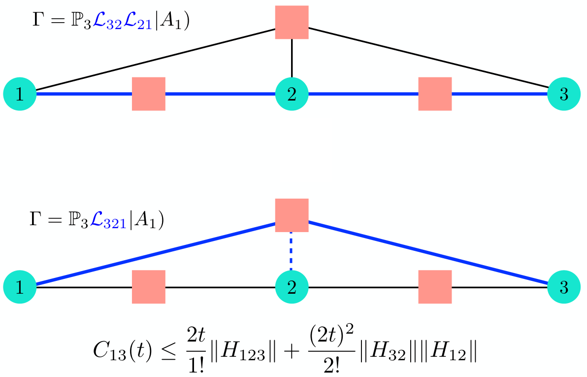
Theorem 3.2 states that operator growth, as measured by $C_{ij}(t)$, is bounded by the “weight” of all irreducible paths from $i$ to $j$. This also immediately implies the following corollary:

References

- [1] Y. Sekino and L. Susskind. “Fast scramblers”, Journal of High Energy Physics 10 065 (2008), arXiv:0808.2096.
- [2] P. Hayden and J. Preskill. “Black holes as mirrors: quantum information in random subsystems”, Journal of High Energy Physics 09 120 (2007), arXiv:0708.4025.
- [3] D. Dieks. “Communication by EPR devices”, Physics Letters A92 271 (1982).
- [4] W. Wootters and W. Zurek. “A single quantum cannot be cloned”, Nature 299 802 (1982).
- [5] G. Bentsen, Y. Gu, and A. Lucas. “Fast scrambling on sparse graphs”, Proceedings of the National Academy of Sciences 116 6689 (2019), arXiv:1805.08215.
- [6] M. Gärttner, J. G. Bohnet, A. Safavi-Naini, M. L. Wall, J. J. Bollinger, and A. M. Rey. “Measuring out-of-time-order correlations and multiple quantum spectra in a trapped-ion quantum magnet”, Nature Physics 13 781 (2017), arXiv:1608.08938.
- [7] J. Li, R. Fan, H. Wan, B. Ye, B. Zeng, H. Zhai, X. Peng, and J. Du. “Measuring out-of-time-ordered correlators on a nuclear magnetic resonance quantum simulator”, Physical Review X7 031011 (2017), arXiv:1609.01246.
- [8] S. H. Shenker and D. Stanford. “Black holes and the butterfly effect”, Journal of High Energy Physics 03 067 (2014), arXiv:1306.0622.
- [9] N. Lashkari, D. Stanford, M. Hastings, T. Osborne, and P. Hayden. “Towards the fast scrambling conjecture”, Journal of High Energy Physics 04 022 (2013), arXiv:1111.6580.
- [10] E. H. Lieb and D. Robinson. “The finite group velocity of quantum spin systems”, Communications in Mathematical Physics 28 251 (1972).
- [11] D. Poulin. “Lieb-Robinson bound and locality for general Markovian quantum dynamics”, Physical Review Letters 104 190401 (2010), arXiv:1003.3675.
- [12] M. Hastings and T. Koma. “Spectral gap and exponential decay of correlations”, Communications in Mathematical Physics 265 781 (2006), arXiv:math-ph/0507008.
- [13] F. J. Dyson. “Divergence of perturbation theory in quantum electrodynamics”, Physical Review 85 531 (1952).
- [14] S. Sachdev and J. Ye. “Gapless spin-fluid ground state in a random quantum Heisenberg magnet”, Physical Review Letters 70 3339 (1993), arXiv:cond-mat/9212030.
- [15] J. Maldacena and D. Stanford. “Comments on the Sachdev-Ye-Kitaev model”, Physical Review D94 106002 (2016), arXiv:1604.07818.
- [16] A. Kitaev and S. J. Suh. “The soft mode in the Sachdev-Ye-Kitaev model and its gravity dual”, Journal of High Energy Physics 05 183 (2018), arXiv:1711.08467.
- [17] D. A. Roberts, D. Stanford, and A. Streicher. “Operator growth in the SYK model”, Journal of High Energy Physics 06 122 (2018), arXiv:1802.02633.
- [18] R. J. Riddell Jr. “The number of Feynman diagrams”, Physical Review 91 1243 (1953).
- [19] J. Polchinski. “Combinatorics of boundaries in string theory”, Physical Review D50 6041 (1994), arXiv:hep-th/9407031.
- [20] P. Saad, S. H. Shenker, and D. Stanford. “JT gravity as a matrix integral”, arXiv:1903.11115.
- [21] J. M. Maldacena. “The large limit of superconformal field theories and supergravity”, Advances in Theoretical and Mathematical Physics 2 231 (1998), arXiv:hep-th/9711200.
- [22] F. R. Kschischang, B. J. Frey, and H-A. Loeliger. “Factor graphs and the sum-product algorithm”, IEEE Transactions on Information Theory 47 498 (2001).
- [23] J. R. Stallings. “Topology of finite graphs”, Inventiones Mathematicae 71 551 (1983).
- [24] F. R. K. Chung. Spectral Graph Theory, (American Mathematical Society, 1997).
- [25] Z. Wang and K. R. A. Hazzard. “Tightening the Lieb-Robinson bound in locally interacting systems”, PRX Quantum 1 010303 (2020), arXiv:1908.03997.
- [26] Norio Konno. Limit theorem for continuous-time quantum walk on the line. Physical Review E, 72(2), Aug 2005.
- [27] A. Lucas. “Non-perturbative dynamics of the operator size distribution in the Sachdev-Ye-Kitaev model”, Journal of Mathematical Physics 61 081901 (2020), arXiv:1910.09539.
- [28] T. Kadowaki and H. Nishimori. “Quantum annealing in the transverse Ising model,” Physical Review E58 5355 (1998), arXiv:cond-mat/9804280.
- [29] E. Farhi, J. Goldstone, S. Gutmann, J. Lapan, A. Lundgren, and D. Preda. “A quantum adiabatic evolution algorithm applied to random instances of an NP-complete problem,” Science 292 472 (2001), arXiv:quant-ph/0104129.
- [30] A. Lucas. “Quantum many-body dynamics on the star graph”, arXiv:1903.01468.
- [31] L. Arrachea and M. J. Rozenberg. “The infinite-range quantum random Heisenberg magnet”, Physical Review B65 224430 (2002), arXiv:cond-mat/0203537.
- [32] P. Flajolet and R. Sedgewick. Analytic Combinatorics, (Cambridge University Press, 2009).
- [33] J. Schmidt-Pruzan and E. Shamir. “Component structure in the evolution of random hypergraphs”, Combinatorica 5 81 (1985).
- [34] C. M. Bender and S. A. Orszag. Asymptotic Methods and Perturbation Theory, (Springer, 2010).
- [35] C-F. Chen. “Concentration of OTOC and Lieb-Robinson velocity in random Hamiltonians”, arXiv:2103.09186.
- [36] E. Witten. “An SYK-like model without disorder”, arXiv:1610.09758.
- [37] R. Gurau. “The complete expansion of a SYK-like tensor model”, Nuclear Physics B916 386 (2017), arXiv:1611.04032.
- [38] I. R. Klebanov and G. Tarnopolsky. “Uncolored random tensors, melon diagrams, and the SYK models”, Physical Review D95 046004 (2017), arXiv:1611.08915.
- [39] S. S. Gubser, C. Jepsen, Z. Ji, and B. Trundy. “Higher melonic theories”, Journal of High Energy Physics 09 049 (2018), arXiv:1806.04800.
- [40] A. Lucas and A. Osborne. “Operator growth bounds in a cartoon matrix model”, Journal of Mathematical Physics 61 122301 (2020), arXiv:2007.07165.
- [41] A. Lucas. “Operator size at finite temperature and Planckian bounds on quantum dynamics”, arXiv:1809.07769.
- [42] J. Maldacena, S. H. Shenker, and D. Stanford. “A bound on chaos”, Journal of High Energy Physics 08 106 (2016), arXiv:1503.01409.
- [43] X-L. Qi and A. Streicher. “Quantum epidemiology: operator growth, thermal effects, and SYK”, arXiv:1810.11958.
- [44] X. Han and S. A. Hartnoll. “Quantum scrambling and state dependence of the butterfly velocity”, arXiv:1812.07598.
- [45] X. Chen, Y. Gu, and A. Lucas. “Many-body quantum dynamics slows down at low density”, SciPost Physics 9 071 (2020), arXiv:2007.10352.
- [46] Q. Zhuang, T. Schuster, B. Yoshida, and N. Y. Yao. “Scrambling and complexity in phase space”, arXiv:1902.04076.
- [47] B. Nachtergaele, H. Raz, B. Schlein, and R. Sims. “Lieb-Robinson bounds for harmonic and anharmonic lattices”, Communications in Mathematical Physics 286 1073 (2009), arXiv:0712.3820.
- [48] T. Banks, W. Fischler, S. H. Shenker, and L. Susskind. “M theory as a matrix model: a conjecture”, Physical Review D55 5112 (1997), arXiv:hep-th/9610043.
- [49] A. Nahum, S. Vijay, and J. Haah. “Operator spreading in random unitary circuits”, Physical Review X8 021014 (2018), arXiv:1705.08975.
- [50] C. W. von Keyserlingk, T. Rakovsky, F. Pollmann, and S. L. Sondhi. “Operator hydrodynamics, OTOCs, and entanglement growth in systems without conservation laws”, Physical Review X8 021013 (2018), arXiv:1705.08910.
- [51] M. C. Tran, Guo A, Y, Y. Su, J. R. Garrison, Z. Eldredge, M. Foss-Feig, A. M. Childs, and A. V. Gorshkov. “Locality and Digital Quantum Simulation of Power-Law Interactions”, Physical Review X9 031006 (2019), arXiv:1808.05225.
- [52] Chi-Fang Chen and Andrew Lucas. “Finite speed of quantum scrambling with long range interactions”, Physical Review Letters 123 250605 (2019), arXiv:1907.07637.
- [53] T. Kuwahara and K. Saito. “Strictly Linear Light Cones in Long-Range Interacting Systems of Arbitrary Dimensions”, Physical Review X10 031010 (2020), arXiv:1910.14477.
- [54] M. C. Tran, A. Deshpande, A. Y. Guo, A. Lucas, and A. V. Gorshkov. “Optimal state transfer and entanglement generation in power-law interacting systems”, arXiv:2010.02930.
- [55] M. C. Tran, C-F. Chen, A. Ehrenberg, A. Y. Guo, A. Deshpande, Y. Hong, Z-X. Gong, A. V. Gorshkov, and A. Lucas. “Hierarchy of Linear Light Cones with Long-Range Interactions”, Physical Review X10 031009 (2020), arXiv:2001.11509.
- [56] T. Kuwahara and K. Saito. “Absence of Fast Scrambling in Thermodynamically Stable Long-Range Interacting Systems”, Physical Review Letters 126 030604 (2021), arXiv:2009.101244=.
- [57] C-F. Chen and A. Lucas. “Optimal Frobenius light cone in spin chains with power-law interactions”, arXiv:2105.09960.
- [58] D. E. Parker, X. Cao, A. Avdoshkin, T. Scaffidi, and E. Altman. “A Universal Operator Growth Hypothesis”, Physical Review X9 041017 (2019), arXiv:1812.08657.
- [59] A. Avdoshkin and A. Dymarsky. “Euclidean operator growth and quantum chaos”, Physical Review Research 2 043234 (2020), arXiv:1911.09672.