Constraints on Flavor-Diagonal Non-Standard Neutrino Interactions from Borexino Phase-IIPreprint: IP/BBSR/2019-2The Borexino CollaborationarXiv: 1905.03512

Within the SM, the elastic scattering of $\nu_{\alpha}$ ($\alpha=e,\mu,\tau$) on electrons proceeds via $Z$-exchange (Neutral Current, NC) and, for $\nu_{e}$, also via $W$-exchange (Charged Current, CC). At momentum transfers relevant for Borexino ($Q^{2}\ll M_{W}^{2},M_{Z}^{2}$), the CC and NC processes are well approximated by the point interaction:

where we have used the Fierz transformation Fierz:1937; Nieves:2003in to rewrite the CC interaction into NC form, and we follow the notation of the Review of Particle Physics Erler:2018 for the NC coupling constants. The tree-level values of these couplings are

Combining () and (4) we have

with

For a monochromatic neutrino of energy $E$ and flavor $\alpha$ scattering off an electron at rest, the interaction (9) predicts the spectrum of the kinetic energy $T$ of the recoiling electrons to be tHooft:1971ucy; Bahcall:1986pf

where neutrino masses have been neglected and $T$ is constrained as:

The tree-level expression for the cross section given in Eq. (12) is modified by radiative corrections Ram:1967zza; Marciano:1980pb; Sarantakos:1982bp; Wheater:1982yk; Bahcall:1995mm; Passera:2000ug. In the present analysis, these corrections are accounted for following the 1995 paper of Bahcall, Kamionkowski, and Sirlin Bahcall:1995mm with parameters updated to reflect the more recently available experimental data, e.g. the Higgs mass, and $\hat{s}_{Z}^{2}=0.23129$.²² 2 $\hat{s}_{Z}^{2}$ denotes the $\overline{\text{MS}}$ value of $\sin^{2}\theta_{W}$ at the $Z$-mass scale. The value of $\hat{s}_{Z}^{2}=0.23129\pm 0.00005$ is from the 2016 Review of Particle Physics Patrignani:2016xqp. It has subsequently been updated to $\hat{s}_{Z}^{2}=0.23122\pm 0.00003$ in the 2018 Review of Particle Physics Erler:2018; Tanabashi:2018oca, but this difference is too small to be of relevance to the analysis of this paper. Borexino does not distinguish between muon- and tau-neutrinos, and the difference in radiative corrections for the two flavors is consequently ignored: the radiative corrections to $\nu_{\tau}$ were set to be the same as those for the $\nu_{\mu}$. The sizes of these radiative corrections are generally small compared to the experimental precision of Borexino with the exception of the recent 2.7% measurement of the ${}^{7}\text{Be}$ solar neutrino flux Agostini:2018uly. The effect of radiative corrections has a comparable magnitude, resulting in a $\sim$2% reduction of the total cross section for $\nu_{e}$, and a 1.2% increase for $\nu_{\mu/\tau}$ Bahcall:1995mm. Nevertheless, they have little impact on the present analysis.

In addition to the SM interactions presented above, many models of physics beyond the Standard Model (BSM) predict new interactions of the neutrinos with the other SM fermions Antusch:2008tz; Gavela:2008ra; Malinsky:2008qn; Ohlsson:2009vk; Medina:2011jh; Farzan:2015doa; Farzan:2015hkd; Farzan:2016wym; Blennow:2016jkn; Deniz:2017zok; Pospelov:2017kep. Phenomenologically, such non-standard interactions (NSI’s) of the NC type are described by the Lagrangian density Berezhiani:2001rs; Ohlsson:2012kf

where $\alpha,\beta=e,\mu,\tau$ label the neutrino flavor, $f$ and $f^{\prime}$ are leptons or quarks of the same charge but not necessarily the same flavor, $C$ is the chirality of the $ff^{\prime}$ current ($L$ or $R$), and $\varepsilon_{\alpha\beta}^{ff^{\prime}C}$ is a dimensionless coupling parametrizing the strength of the NSI interaction normalized to $G_{F}$. Allowing $\alpha\neq\beta$ and $f\neq f^{\prime}$ in (14) accounts for possible flavor-changing NSI’s. Hermiticity of the interaction demands

where the asterisk denotes complex conjugation. In the current analysis, however, we restrict our attention to the flavor-diagonal case $f=f^{\prime}=e$ and $\alpha=\beta$, and denote $\varepsilon_{\alpha}^{C}\equiv\varepsilon_{\alpha\alpha}^{eeC}$. Borexino, relying on neutrino-electron elastic scattering, is particularly sensitive to this type. A discussion on BSM models which may produce such NSI’s can be found in Refs. Berezhiani:2001rs; Davidson:2003ha; Barranco:2007ej; Farzan:2017xzy ³³ 3 Before the confirmation of neutrino oscillations by the KamLAND experiment, NSI’s with massless neutrinos had also been invoked to address the solar neutrino anomaly. See Refs. Guzzo:1991hi; Guzzo:1991cp; valle1987resonant; Roulet:1991sm; Barger:1991ae; Guzzo:2001mi..

NSI’s can affect neutrino production, detection, and propagation. Inside the Sun, the flavor diagonal NSI’s under consideration contribute to the production of same-flavor $\nu\overline{\nu}$ pairs via photo-production ($\gamma e\to e\nu\overline{\nu}$), $\nu\overline{\nu}$-Bremsstrahlung (the photon leg in $\gamma e\to e\nu\overline{\nu}$ is anchored on an ion or another electron), etc. Vitagliano:2017odj. However, the energies of the neutrinos and anti-neutrinos produced by these processes are expected to be in the few keV range, well below the $\sim$50 keV detection threshold of Borexino Agostini:2018uly.

At detection, $\varepsilon_{\alpha}^{L/R}$ ($\alpha=e,\mu,\tau$) shift the coupling constants that appear in the expression for the differential cross section, Eq. (12):

Strong bounds on $\varepsilon_{\mu}^{L/R}$ had already been obtained by the $\nu_{\mu}e$ scattering experiment CHARM II Vilain:1994qy, namely $-0.025<\varepsilon_{\mu}^{L}<0.03$ and $-0.027<\varepsilon_{\mu}^{R}<0.03$ at 90% C.L. Davidson:2003ha.⁴⁴ 4 These are one-parameter-at-a-time bounds. One-parameter projections of two-parameter bounds at 90% C.L. are given as $-0.033<\varepsilon_{\mu}^{L}<0.055$ and $-0.040<\varepsilon_{\mu}^{R}<0.053$ in Ref. Barranco:2007ej. Therefore, we restrict our attention to the remaining four parameters: $\varepsilon_{e}^{L/R}$ and $\varepsilon_{\tau}^{L/R}$. We do not consider the full 4-dimensional space $\varepsilon_{\alpha}^{L/R}$ ($\alpha=e,\tau$): such a detailed description is not necessary at the current level of sensitivity to NSI’s. Instead, we investigate the $\varepsilon_{e}^{L/R}$ and $\varepsilon_{\tau}^{L/R}$ cases separately, even though – as it will become evident later with (19) and (22) – these groups of parameters cannot be decoupled with Borexino.

The description of how NSI’s affect neutrino propagation can be found in Ref. Bolanos:2008km; Farzan:2017xzy; Friedland:2004pp; Maltoni:2015kca. Let us discuss in some detail what we should expect from their inclusion. Neutrino propagation in matter is only sensitive to the vectorial combinations $\varepsilon_{\alpha}^{V}\equiv\varepsilon_{\alpha}^{L}+\varepsilon_{\alpha}^{R}$. They modify the matter-effect potential in the flavor basis to

where $V(x)=\sqrt{2}G_{F}N_{e}(x)$, and $N_{e}(x)$ is the electron density at location $x$. From a practical point of view, $\varepsilon_{e}^{V}=\varepsilon_{e}^{L}+\varepsilon_{e}^{R}$ and $\varepsilon_{\tau}^{V}=\varepsilon_{\tau}^{L}+\varepsilon_{\tau}^{R}$ can be introduced as a shift in the matter-effect potential $V(x)$ in two-flavor oscillation analysis:

where $\varepsilon^{\prime}=\varepsilon_{\tau}^{V}\sin^{2}\theta_{23}-\varepsilon_{e}^{V}$ Bolanos:2008km. The derivation of this effective potential is given in appendix A, assuming $|\Delta m^{2}_{31}|\gg 2EV(x)$, where $E$ is the neutrino energy. There, it is also shown that the first oscillation resonance occurs at $2EV^{\prime}(x)c_{13}^{2}=2E(1-\varepsilon^{\prime})V(x)c_{13}^{2}\approx\Delta m_{21}^{2}\cos 2\theta_{12}$.

For neutrinos coming from the center of the Sun, where the SSM predicts $N_{e}^{\odot}(r=0)\approx 10^{2}N_{A}=6\times 10^{25}/\mathrm{cm^{3}}$ Bahcall:1987jc; Bahcall:2000nu, the resonance energy is

where for $\Delta m^{2}_{21}\cos 2\theta_{12}$ and $c_{13}^{2}=1-s_{13}^{2}$ we have used the central values of the global averages from Ref. Esteban:2016qun.

As the electron density $N_{e}^{\odot}(r)$ decreases towards the surface of the Sun, $r\to R_{\odot}$, the resonance energy $E_{res}^{\odot}(r)$ will increase. The presence of non-zero $\varepsilon^{\prime}$ will also shift the resonance energy: positive $\varepsilon^{\prime}$ to higher values and negative $\varepsilon^{\prime}$ to lower values.

The MSW effect Wolfenstein:1977ue; Wolfenstein:1979ni; Mikheev:1986gs; Mikheev:1986wj in the energy range $E\gtrsim E_{res}^{\odot}(r)$ ensures a well-defined electron neutrino survival probability $P_{ee}(E)$. For lower energies, neutrino oscillates in a vacuum regime, with a smooth $P_{ee}(E)$ change in the transition region between the two regimes of oscillations. Since the energy ranges of $pp$, ${}^{7}\text{Be}$, and $pep$ neutrinos are below the resonance, the influence of matter effect for those components is small compared to that for ${}^{8}\text{B}$ neutrinos.

The mass density at the center of the Earth according to the Preliminary Reference Earth Model (PREM) PREM:1981 is $\rho(r=0)\approx 13\,\mathrm{g/cm^{3}}$, which gives us an estimate of the electron density there as $N_{e}^{\oplus}(r=0)\approx N_{A}\,\rho(r=0)/2=4\times 10^{24}/\mathrm{cm^{3}}$. So the resonance energy of the neutrinos at the Earth’s center is

and $E_{res}^{\oplus}(r)$ will grow larger as the electron density decreases toward the surface of the Earth, $r\to R_{\oplus}$. From this, one can expect matter effects due to the Earth to be small for all solar neutrino components.⁵⁵ 5 For ${}^{8}\text{B}$ neutrinos, the day-night asymmetry for LMA-MSW has been predicted to be a few percent deGouvea:1999xe; Bahcall:2001cb, and this has been confirmed experimentally by Super-Kamiokande Fukuda:1998rq; Smy:2003jf and SNO Ahmad:2002ka; Aharmim:2005gt. The sensitivity of Borexino is insufficient to detect this day-night asymmetry. Indeed, the day-night asymmetry at Borexino for the $\varepsilon^{\prime}=0$ case has been predicted to be a mere fraction of a percent Aleshin:2011hu; Ioannisian:2015qwa, and Borexino reports $A_{dn}^{{}^{7}\text{Be}}=0.001\pm 0.012\text{(stat)}\pm 0.007\text{(syst)}$ in Ref. Bellini:2011yj. A negative value of $\varepsilon^{\prime}$ could, of course, lower the resonance energy and affect this prediction but due to the difference in the energy scales of Eqs. (20) and (21), one expects the effect of $\varepsilon^{\prime}$ would appear in the Sun first.

Figure 1 illustrates the effect of LMA-MSW on $P_{ee}(E)$ for several representative values of $\varepsilon^{\prime}$. NSI’s with $\varepsilon^{\prime}>0$ enhance $P_{ee}(E)$. For $\varepsilon^{\prime}<0$ case, $P_{ee}(E)$ is reduced. According to Eq. (19), as $\varepsilon^{\prime}\to 1$, the matter effect potential vanishes and the $P_{ee}(E)$ tends to Vacuum-LMA scenario that assumes all solar neutrinos are oscillating in the vacuum regime. For the range between $\varepsilon^{\prime}=-0.5$ and $\varepsilon^{\prime}=0.5$, the theoretically predicted shift of $P_{ee}(E)$ is within the error bars of the experimentally determined values of Borexino. The 90% C.L. contours obtained in the present analysis are located almost entirely in this range (see figures 6 and 7). Therefore, the effects of NSI’s at propagation are not particularly strong, and the sensitivity to NSI’s is almost entirely provided at detection.

The objective of this analysis is to investigate the sensitivity of Borexino to the NSI parameters $\varepsilon_{e}^{L/R}$ and $\varepsilon_{\tau}^{L/R}$. In contrast to the analysis of Ref. Agostini:2018uly, in which the $\nu e$ couplings were fixed to those of the SM and the count rates of $pp$, ${}^{7}\mathrm{Be}$, and $pep$ neutrinos were fit to the data, we allow the couplings to float, assuming the SSM neutrino fluxes with either the HZ- or LZ-SSM values (table 1).

We have argued in the previous section that $\varepsilon_{e}^{L/R}$ and $\varepsilon_{\tau}^{L/R}$ affect neutrino propagation and detection: (i) the propagation through a shift in the matter-effect potential, Eq. (19), leading to a modification in the expected $\nu_{e}$ survival probability $P_{ee}(E)$, and (ii) the detection through shifts in the effective chiral coupling constants, Eqs. (16) and (17), leading to modifications in the electron recoil spectra $d\sigma_{\alpha}/dT$ ($\alpha=e,\tau$), Eq. (12).

Four solar neutrino components are considered in this analysis: $pp$, ${}^{7}\text{Be}$, $pep$, and CNO.⁶⁶ 6 In the present analysis, we look for deviations from the SSM + LMA-MSW predictions, so the CNO neutrino flux, together with the other three component fluxes, are simply fixed to those predicted by either the HZ- or LZ-SSM. The SSM Bahcall:1986pf; Bahcall:1987jc; Bahcall:2000nu; Vinyoles:2016djt predicts the energy spectra and fluxes of these neutrinos, which we denote as $d\lambda_{\nu}/dE$ and $\Phi_{\nu}$, where the subscript $\nu$ labels the neutrino component.

The monochromatic ${}^{7}\text{Be}$-component plays a fundamental role in this analysis. Both the shape and the normalization of the electron-recoil spectrum is well-constrained in the fit. Together with the 6%-uncertainty in the theoretical ${}^{7}\text{Be}$ neutrino flux, it provides the highest sensitivity to NSI’s among all the neutrino components. We do not use ${}^{8}\text{B}$ neutrinos to place bounds on NSI’s. The rate of ${}^{8}\text{B}$ neutrino events cannot be determined with the spectral fit used in this analysis, being small and hidden by backgrounds in the energy region considered. Moreover, the relatively large 12%-uncertainty on the ${}^{8}\text{B}$ neutrino flux predicted by the SSM limits its utility for this work.

Taking into account the oscillations of $\nu_{e}$ into $\nu_{\mu}$ and $\nu_{\tau}$, the recoil spectrum for each solar neutrino component is given by

Here, $N_{e}$ is the number of electrons in the fiducial volume of the detector, $s_{23}^{2}\equiv\sin^{2}\theta_{23}$, and $c_{23}^{2}\equiv\cos^{2}\theta_{23}$. $\Phi_{\nu}$ is the expected total flux of solar neutrino component $\nu$ at the Earth, and $d\lambda_{\nu}/dE$ is the corresponding differential neutrino energy spectrum. $P_{ee}(E)$ is the solar-$\nu_{e}$ survival probability to which NSI effects at propagation have been added. The effect of the NSI’s at detection is included in the differential cross sections $d\sigma_{e}/dT$ and $d\sigma_{\tau}/dT$, with the $\varepsilon_{e}^{L/R}$ and $\varepsilon_{\tau}^{L/R}$ parameters always combined in the recoil spectrum of Eq. (22).

The dependence of the ${}^{7}\text{Be}$ electron recoil spectrum $dR_{\mathrm{Be7}}/dT$ on the NSI’s for several values of $\varepsilon_{e}^{R}$ and $\varepsilon_{e}^{L}$ is illustrated in figure 2. Note that $\varepsilon_{e}^{L}$ mostly modifies the normalization of the spectrum, while $\varepsilon_{e}^{R}$ modifies its slope. $\varepsilon_{\tau}^{L}$ and $\varepsilon_{\tau}^{R}$ require much larger magnitudes to achieve the same effects due to the smaller contribution of $\nu_{\tau}$ to $dR_{\mathrm{Be7}}/dT$.

Integrating Eq. (22), one obtains a relation between the total experimental event rate $R_{\nu}$, the solar neutrino flux $\Phi_{\nu}$, and the total cross section $\langle\sigma_{\nu}\rangle$:

NSI effects at propagation and detection are both included in the total cross section $\langle\sigma_{\nu}\rangle$. Denoting the total cross section in the absence of NSI’s as $\langle\sigma_{\nu}\rangle_{\mathrm{SM}}$, we plot the change in the ratio $\langle\sigma_{\nu}\rangle/\langle\sigma_{\nu}\rangle_{\mathrm{SM}}$ for the ${}^{7}\mathrm{Be}$ neutrinos due to the presence of $\varepsilon_{e}^{L}$ and $\varepsilon_{e}^{R}$ in figure 3. Again, we see that $\varepsilon_{e}^{L}$ affects the normalization of the cross section, while $\varepsilon_{e}^{R}$ does not. Thus $\varepsilon_{e}^{L}$ is mostly constrained by the normalization of the cross section, while $\varepsilon_{e}^{R}$ is mostly constrained by the shape of the recoil spectrum.

We performed the selection of the events according to Ref. Agostini:2018uly, using a spherical fiducial volume to which the top and bottom polar regions are cut off: $R<2.8\,\text{m}$, and $-1.8\,\text{m}<z<2.2\,\text{m}$. To model the detector response, we use the analytical model of the Borexino detector discussed in detail in Ref. Agostini:2017ixy. The model uses the number of triggered PMT’s, $N_{p}^{\,dt_{1}}$, within a fixed time interval $dt_{1}=230\,\mathrm{ns}$ as the estimator of the electron recoil energy $T$. Various model parameters have been fixed utilizing independent measurements, or tuned using the Borexino Monte Carlo agostini2018monte and calibrations back2012borexino, while some have been left free to float in the fit. The floating parameters include (i) the light yield, which determines the energy scale, (ii) two parameters for energy resolution, (iii) two parameters for the position and the width of the ${}^{210}\text{Po}$-$\alpha$ peak, and (iv) one parameter for the starting point of the ${}^{11}\text{C}$ $\beta^{+}$-spectrum. The detector response function convoluted with the cross section $dR_{\nu}/dT$ provides the functional form to be fit to the data.

Throughout the minimization procedure, the neutrino oscillation parameters are fixed to the central values of the global fit to all oscillation data given in Ref. Esteban:2016qun⁷⁷ 7 Strictly speaking, to use the Borexino data to constrain possible new physics effects we should not be comparing the data to the global average of Ref. Esteban:2016qun, which includes both Borexino Phase-I and Phase-II data in its fit.However, the numerical difference from the global average of Ref. Capozzi:2016rtj, which includes neither Borexino Phase I nor Phase II data, is small and does not affect the present analysis.. Their uncertainties are directly propagated as the uncertainties of predicted neutrino rates. More details on how the uncertainties are treated can be found in section 3.4.

For the $\varepsilon_{e}^{L/R}$ analysis, we only need

which are valid for any choice of neutrino mass hierarchy.

It is worthwhile to mention that the measurements of $\theta_{12}$ and $\Delta m_{21}^{2}$ from the global oscillation data may be altered if we consider NSI’s in the fit. The solar neutrino experiments such as Super-Kamiokande and SNO provide crucial information on $\theta_{12}$ and $\Delta m_{21}^{2}$, and at the same time they are sensitive to the same NSI’s in propagation and detection that we consider in this paper. However, the reactor experiment KamLAND is unaffected by flavor-diagonal neutral current NSI’s involving neutrinos and electrons. Therefore, when we consider the KamLAND data along with the solar neutrino data mostly coming from Super-Kamiokande and SNO, the solar oscillation parameters $\theta_{12}$, $\Delta m_{21}^{2}$ remain robust even in the presence the NSI’s discussed in this paper. In fact, it was shown in Ref. Bolanos:2008km that Super-Kamiokande and SNO can place competitive constraints on $\varepsilon_{e}^{L}$ and $\varepsilon_{e}^{R}$ with the help of KamLAND data which provides NSI-independent measurement of $\theta_{12}$ and $\Delta m_{21}^{2}$. Note also that for the $\varepsilon_{e}^{L/R}$ analysis $d\sigma_{\mu}/dT=d\sigma_{\tau}/dT$ when $\varepsilon_{\tau}^{L/R}=0$, and Borexino is insensitive to the value of $\theta_{23}$.

For the $\varepsilon_{\tau}^{L/R}$ analysis, we also need to specify $\theta_{23}$. The 1$\sigma$ ranges given in Ref. Esteban:2016qun for Normal and Inverted Hierarchies are

It is easy to see that $\sin^{2}\theta_{23}$ is included linearly in expression (22), and the sensitivity to $\varepsilon_{\tau}^{L/R}$ is proportional to its value. To obtain a conservative limit, we fix $\sin^{2}\theta_{23}$ to the NH value and propagate its uncertainty into systematic error together with other oscillation parameters.

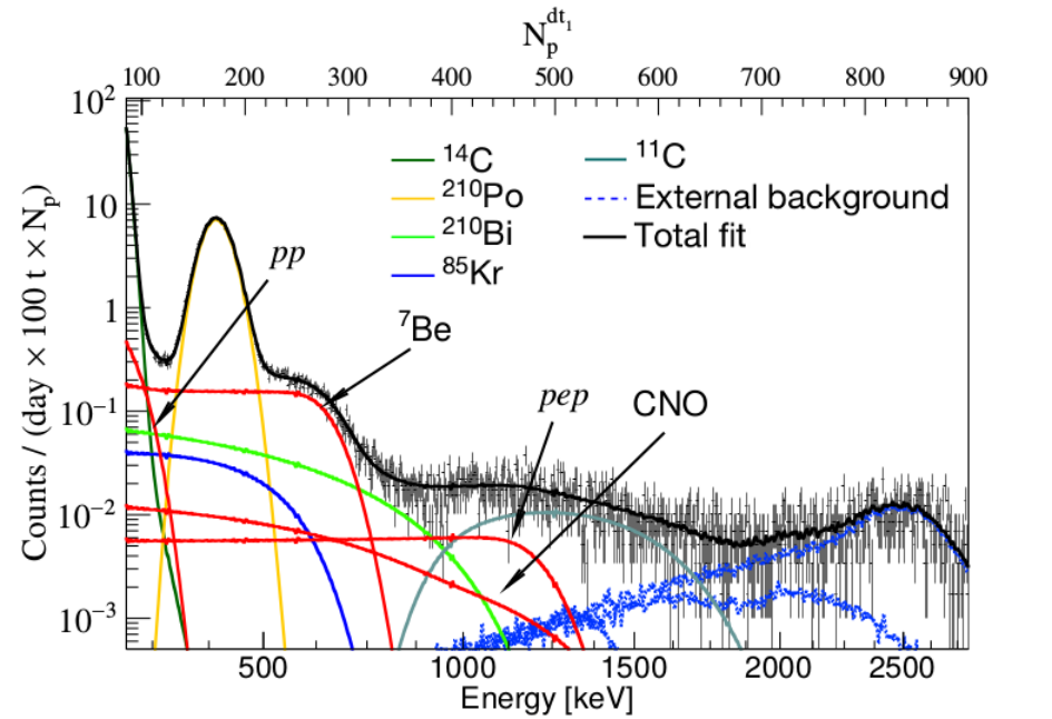
Radioactive contaminants lead to backgrounds that must be clearly understood to extract unambiguous conclusions from the Borexino data. The most recent fit of signal+background to the observed electron recoil spectrum can be found in Ref. Agostini:2018uly, where the SM couplings were assumed and the event rates of three solar neutrino components ($pp$, ${}^{7}\mathrm{Be}$, and $pep$) were allowed to float. An example fit to the experimental spectrum is shown in figure 4. A full description of the Borexino spectral components and backgrounds is found in Ref. Bellini:2013lnn. Here, we focus on the components which are the most relevant for the current analysis:

• •

  At low-energies the $\beta$-emitter ${}^{14}\text{C}$ with $Q=156\>\text{keV}$ is the main background for $pp$ neutrinos ($T_{\max}=261\>\text{keV}$).

  The ${}^{14}\text{C}$ contribution is constrained in the fit with an independent measurement by selection of events with low energy threshold. Since the rate of ${}^{14}\text{C}$ is high compared to the other components, pile-up events need to be taken into account. The detailed data selection and analysis procedures are found in Ref. Bellini:2014uqa.

• •

  Decays of ${}^{85}\text{Kr}$ ($\beta^{-}$, $Q=687\>\text{keV}$), ${}^{210}\text{Bi}$ ($\beta^{-}$, $Q=1160\>\text{keV}$), and ${}^{210}\text{Po}$ ($\alpha$, $E=5.3\>\text{MeV}$) are the main backgrounds for the detection of the electron recoil spectra from the two mono-energetic ${}^{7}\text{Be}$ solar neutrino lines ($E=384\>\text{keV}$ and $862\>\text{keV}$).

  The ${}^{210}\text{Po}$ $\alpha$-decay peak ($E=5.3$ MeV) appears at $\sim$400 keV due to ionization quenching effects in the liquid scintillator. While very intense with respect to the other spectral components, the shape of the polonium peak is very distinct, well understood, and easily separable in the fit.

  The $\beta$ spectra of ${}^{210}\text{Bi}$ and ${}^{85}\text{Kr}$ overlap with the ${}^{7}\text{Be}$ electron-recoil spectrum leading to a modification of its shape. This reduces the sensitivity to the right-handed NSI parameter $\varepsilon_{\alpha}^{R}$. The background from ${}^{85}\text{Kr}$ is quite serious since the shape of its $\beta$-spectrum and its end-point are close to the step-like spectrum of ${}^{7}\text{Be}$.

• •

  Other backgrounds necessary to the fit of the experimental spectrum are cosmogenic $\beta^{+}$ emitter ${}^{11}\text{C}$, and $\gamma$-rays from ${}^{208}\text{Tl}$, ${}^{214}\text{Bi}$, and ${}^{40}\text{K}$ from components of the detector external to the scintillator.

The fitting procedure consists of the multivariate maximization of the composite likelihood function $\mathcal{L}(\vec{k}\,|\varepsilon,\vec{\theta})$, specifically developed to be able to detect $pep$, and CNO neutrinos hidden by the cosmogenic $\beta^{+}$ ${}^{11}\text{C}$ and external backgrounds:

Here, $\varepsilon$ is the NSI parameter we would like to constrain, and the vector $\vec{\theta}$ collectively represents all the other model parameters of the fit, including the rates of the four solar neutrino components $R_{\nu}$, the intensities of the backgrounds, detector response parameters, etc., and $\vec{k}$ denotes the set of experimental data.

In order to deal with ${}^{11}\text{C}$ background, the dataset was divided into two parts by the so-called three-fold coincidence (TFC) technique (Refs. Bellini:2013lnn; Agostini:2017ixy). The method tags events correlated in space and time with a parent muon and one or several neutrons often produced together with ${}^{11}\text{C}$. The division is based on the probability for an event to be ${}^{11}\text{C}$ and results in ${}^{11}\text{C}$-depleted (TFC-subtracted) and ${}^{11}\text{C}$-enriched (TFC-tagged) data samples. The first and the second factors of Eq. (28) represent two separate likelihoods for TFC-subtracted and TFC-tagged experimental spectra, respectively. They are a standard Poisson likelihood:

where $N_{E}$ is the number of energy bins, $\lambda_{i}(\varepsilon,\vec{\theta})$ is the expected number of events in the $i$-th bin for a given set of parameters $\varepsilon$ and $\vec{\theta}$, and $k_{i}$ is the measured number of events in the $i$-th bin.

The residual events from ${}^{11}\text{C}$ in the TFC-subtracted spectrum can be discriminated by the algorithm incorporated into $\mathcal{L}_{P}(\vec{k}\,|\vec{\theta})$. To account for external backgrounds which penetrate into the fiducial volume, the fit of the spatial radial distribution of events is incorporated by $\mathcal{L}_{R}(\vec{k}\,|\vec{\theta})$. The more detailed description of the likelihood function and the fitting procedure can be found in section XXI of Ref. Bellini:2013lnn, and in Ref. Agostini:2017ixy.

We add penalty factors to $\mathcal{L}(\vec{k}\,|\varepsilon,\vec{\theta})$ to constrain the four neutrino rates to the SSM prediction Bahcall:1986pf; Bahcall:1987jc; Bahcall:2000nu; Vinyoles:2016djt:

where $\theta_{\nu}$ represents the floating value of $R_{\nu}$. $R_{\nu}^{\mathrm{SSM}}(\varepsilon)$ is the expected rate calculated by (23) from the prediction of the SSM with either the HZ or LZ assumption and for a given set of NSI parameters $\varepsilon$, and oscillation parameters fixed to their central values. $\delta_{R_{\nu}^{\mathrm{SSM}}}(\varepsilon)$ is its uncertainty stemming from theoretical uncertainties of the SSM and systematic uncertainties on the estimated number of target electrons $N_{e}$, on the fiducial volume, and on the oscillation parameters.

Performing a series of fits for different values of $\varepsilon$, one can obtain a likelihood probability distribution

where $\vec{\theta}_{\max}(\varepsilon)$ is the set of values of $\vec{\theta}$ that maximizes the likelihood for a particular value of $\varepsilon$. The upper $\varepsilon_{\mathrm{up}}$ and lower $\varepsilon_{\mathrm{low}}$ bounds for a given confidence level (C.L.) can be numerically obtained by integrating the tails of the following distribution:

For the two dimensional case when two parameters ($\varepsilon_{1},\varepsilon_{2}$) are under investigation, the confidence region is formed by the isocontour $p_{0}=\mathrm{const}$, defined though the integral over the excluded region:

where $p(\varepsilon_{1},\varepsilon_{2})<p_{0}$ stands for the region outside of the isocontour $p_{0}$.

In this section, we present our results. Left panels of figure 5 shows the one-dimensional log-likelihood profiles for $\varepsilon_{e}^{R}$ (red curve) and $\varepsilon_{e}^{L}$ (blue curve) assuming HZ- (top panel) and LZ-SSM (bottom panel). Right panels of figure 5 portrays the same for $\varepsilon_{\tau}^{R}$ (red curve) and $\varepsilon_{\tau}^{L}$ (blue curve).

Let us first discuss the HZ-SSM case (top panels). One can see that the sensitivity of Borexino to the NSI parameter $\varepsilon_{e}^{L}$ is more pronounced as compared to its sensitivity to $\varepsilon_{e}^{R}$ (see top left panel of figure 5). The main reason behind this is that the normalization of neutrino events is well determined by the fit, which in turn provides competitive constraints for $\varepsilon_{e}^{L}$. In contrast, the fit still permits quite a wide range for $\varepsilon_{e}^{R}$, since the possible modification in the shape of the event spectra due to non-zero $\varepsilon_{e}^{R}$ can be easily mimicked by the principle background components (mainly ${}^{85}\text{Kr}$) discussed above. Note that the minima of the one-dimensional log-likelihood profiles for $\varepsilon_{e}^{R}$ (red line in left panel) and $\varepsilon_{\tau}^{R}$ (red line in right panel) are slightly deviated from zero, but, needless to mention that these deviations are statistically insignificant.

The one-dimensional log-likelihood profiles for both $\varepsilon_{\tau}^{R}$ and $\varepsilon_{\tau}^{L}$ look non-parabolic in the top right panel of figure 5. In particular, $\varepsilon_{\tau}^{L}$ demonstrates one extra minimum around $\varepsilon_{\tau}^{L}$ $\approx$ 0.6, which is slightly disfavored at $\Delta\chi^{2}=-2\Delta lnL\approx 1.5$ as compared to the global minimum at $\varepsilon_{\tau}^{L}=0$. This minimum originates due to the approximate $\tilde{g}_{\alpha L}\leftrightarrow-\tilde{g}_{\alpha L}$ symmetry that Eq. (12) possesses, since the first term in Eq. (12) dominates over the third term Bolanos:2008km. Because of this symmetry, the value of $\tilde{g}_{\tau L}^{2}=(g_{\tau L}+\varepsilon_{\tau}^{L})^{2}$ is the same for $\varepsilon_{\tau}^{L}=0$ and $\varepsilon_{\tau}^{L}=-2g_{\tau L}\approx 0.54$, and therefore, one may expect a local minimum in vicinity of the second point. The presence of the third term in Eq. (12) shifts the position of this local minimum slightly upward to $\varepsilon_{\tau}^{L}\approx 0.64$.

The profiles for the LZ-SSM case (figure 5, bottom panels) are clearly shifted from zero and with respect to the HZ-SSM ones. The main reason for this is that LZ-SSM predicts smaller $\Phi_{{}^{7}\text{Be}}$ compared to HZ-SSM. The smaller flux requires a bigger cross section $\langle\sigma_{{}^{7}\text{Be}}\rangle$ for a given observed experimental rate $R_{{}^{7}\text{Be}}$ (see Eq. 23). As figure 3 illustrates, the total cross section linearly depends on $\varepsilon_{e}^{L}$. Therefore, the minimum for LZ-SSM should be shifted in positive direction of $\varepsilon_{e}^{L}$. For $\varepsilon_{\tau}^{L}$ the minima go in opposite directions due to the same reason. The only difference is that the cross section increases when $\varepsilon_{\tau}^{L}$ goes in negative direction for the first minimum and when $\varepsilon_{\tau}^{L}$ goes up for the second one (see figure 3, right panel). Aforementioned shifts for $\varepsilon_{e}^{L}$ and $\varepsilon_{\tau}^{L}$ profiles induce the shifts for $\varepsilon_{e}^{R}$ and $\varepsilon_{\tau}^{R}$ as well. This will be easy to see later on considering two dimensional profiles (figures 6 and 7).

The 90% C.L. (1 d.o.f.) bounds on the flavor-diagonal NSI parameters obtained using the Borexino Phase-II data are listed in table 2. The first column shows the constraints assuming HZ-SSM for the neutrino fluxes. The second column presents the same considering LZ-SSM. These constraints are obtained varying only one NSI parameter at-a-time, while the remaining three NSI parameters are fixed to zero.

The third column exhibits the bounds obtained by phenomenological analysis with Borexino Phase-I data in Ref. Agarwalla:2012wf. All experimental limits from Borexino Phase-II are better than those previously obtained from the Borexino Phase-I data in Ref. Agarwalla:2012wf. For the sake of comparison, in the forth column, we present the global bounds from Ref. Barranco:2007ej, where the authors analyzed the data from the Large Electron-Positron Collider (LEP) experiment, LSND and CHARM II accelerator experiments, and Irvine, MUNU, and Rovno reactor experiments. The bounds found in the present analysis are quite comparable to the global ones. One may note that the best up-to-date bound for $\varepsilon_{e}^{L}$ was obtained in this work.

We have considered above the sensitivity of the Borexino Phase II data to NSI’s applying the SSM-constraint on the neutrino fluxes. Remarkably, Borexino detector is sensitive to the modification of the shape of ${}^{7}\text{Be}$ electron recoil spectra even if the neutrino fluxes are not constrained by SSM model. Such analysis provides a limit:

As one may see the limit is highly asymmetric, with a large extension for the negative values of $\varepsilon_{e}^{R}$. Such a small sensitivity is induced by backgrounds (mostly ${}^{85}\text{Kr}$) which can easily compensate the modification of electron-recoil spectra.

Now let us consider the two-dimensional case when the allowed region for NSI parameters $\varepsilon_{e}^{L/R}$ is plotted while $\varepsilon_{\tau}^{L}$ and $\varepsilon_{\tau}^{R}$ are fixed to zero (figure 6). Two contours for HZ- (filled) and LZ-SSM (dashed) were obtained. Compared with other experiments sensitive to the same NSI’s, the allowed contours for Borexino in the $\varepsilon_{e}^{L}$-$\varepsilon_{e}^{R}$ plane have a distinct orientation, cf. figure 6. The TEXONO experiment Deniz:2010mp is mostly sensitive to $\varepsilon_{e}^{R}$, while LSND Davidson:2003ha; Auerbach:2001wg is mostly sensitive to $\varepsilon_{e}^{L}$ . Borexino’s contour intersects the allowed regions for both experiments at a certain angle, and the three experiments complement each other. In principle, the overlap of Borexino with TEXONO results in two allowed regions. To exclude the second intersection, the incorporation of the LSND result is necessary.

As it was already explained in the analysis of one-dimensional profiles, the contours for HZ- and LZ-SSM’s are shifted along $\varepsilon_{e}^{L}$-axis. Considering two-dimensional case it is evident that such a shift in $\varepsilon_{e}^{L}$ has to produce also the displacement for $\varepsilon_{e}^{R}$.

The contour for Borexino is extended in the direction of negative $\varepsilon_{e}^{R}$ and $\varepsilon_{e}^{L}$ due to the presence of backgrounds, especially ${}^{85}\text{Kr}$. The shift of the contour for LZ-case with respect to HZ one is due to the change of rate of the backgrounds because of the spectral correlations.

For both HZ- and LZ-SSM cases, the bounds on the left parameter are stronger than the result from LSND. TEXONO Deniz:2010mp is a reactor antineutrino experiment and its bounds are obtained from $\overline{\nu}_{e}e$ scattering. For anti-neutrinos the roles of $\tilde{g}_{eL}$ and $\tilde{g}_{eR}$ are reversed, leading to a stronger bound on $\varepsilon_{e}^{R}$. Due to the approximate symmetry $\tilde{g}_{e}^{R}\leftrightarrow-\tilde{g}_{e}^{R}$ in the anti-neutrino scattering cross section, two separate contours form the allowed region of TEXONO around $\varepsilon_{e}^{R}=0$ and $\varepsilon_{e}^{R}=-2g_{eR}=-2\sin^{2}\theta_{W}\approx-0.5$.

The contour obtained in Ref. Bolanos:2008km is presented by a dashed black line. In this work, the global analysis of several solar neutrino experiments together with KamLAND result was conducted. NSI’s were considered in both detection and propagation. The very first results of Borexino were also included collaboration2007first; Bellini:2008mr; Arpesella:2008mt. Though, as the authors underlined, they did not contribute much in overall sensitivity to NSI’s. As one may see, the present Borexino results are quite complementary to this contour.

The result of Borexino in the $\varepsilon_{\tau}^{L}$-$\varepsilon_{\tau}^{R}$ plane is shown in figure 7. It is similar to that of LEP Barranco:2007ej in excluded area, but it occupies a slightly different region, favoring positive $\varepsilon_{\tau}^{R}$ and negative $\varepsilon_{\tau}^{L}$. NSI’s comparable with the SM neutral current interactions are still allowed.

The result for LZ-SSM is of particular interest. The shift of the minima discussed above and observed in figure 5 (bottom right) transforms the allowed contour (figure 7, dashed dark blue) into two separate regions, one of which is already almost completely excluded by LEP data. So, the remaining allowed region, in this case, is relatively small.

The dotted gray lines in figures 6 and 7 indicate the range for the parameter $\varepsilon^{\prime}$ relevant for NSI’s at propagation. The contours are almost entirely located between $\varepsilon^{\prime}=-0.5$ and $\varepsilon^{\prime}=0.5$. As it was previously shown in section 2.3 (see figure 1), NSI’s at propagation are not very pronounced for these magnitudes of $\varepsilon^{\prime}$ compare to the precision of the the measurements. Thus, the sensitivity of the detector is mostly determined by NSI’s at detection.

References

- (1) SNO collaboration, Q. R. Ahmad et al., Direct evidence for neutrino flavor transformation from neutral current interactions in the Sudbury Neutrino Observatory, Phys. Rev. Lett. 89 (2002) 011301 [nucl-ex/0204008].
- (2) Super-Kamiokande collaboration, K. Abe et al., Solar Neutrino Measurements in Super-Kamiokande-IV, Phys. Rev. D94 (2016) 052010 [1606.07538].
- (3) KamLAND collaboration, K. Eguchi et al., First results from KamLAND: Evidence for reactor anti-neutrino disappearance, Phys. Rev. Lett. 90 (2003) 021802 [hep-ex/0212021].
- (4) KamLAND collaboration, T. Araki et al., Measurement of neutrino oscillation with KamLAND: Evidence of spectral distortion, Phys. Rev. Lett. 94 (2005) 081801 [hep-ex/0406035].
- (5) KamLAND collaboration, S. Abe et al., Precision Measurement of Neutrino Oscillation Parameters with KamLAND, Phys. Rev. Lett. 100 (2008) 221803 [0801.4589].
- (6) L. Wolfenstein, Neutrino Oscillations in Matter, Phys. Rev. D17 (1978) 2369.
- (7) L. Wolfenstein, Neutrino Oscillations and Stellar Collapse, Phys. Rev. D20 (1979) 2634.
- (8) S. P. Mikheyev and A. Yu. Smirnov, Resonance Amplification of Oscillations in Matter and Spectroscopy of Solar Neutrinos, Sov. J. Nucl. Phys. 42 (1985) 913.
- (9) S. P. Mikheev and A. Yu. Smirnov, Resonant amplification of neutrino oscillations in matter and solar neutrino spectroscopy, Nuovo Cim. C9 (1986) 17.
- (10) M. Maltoni and A. Yu. Smirnov, Solar neutrinos and neutrino physics, Eur. Phys. J. A52 (2016) 87 [1507.05287].
- (11) Borexino-SOX collaboration, M. Pallavicini et al., Solar neutrino detectors as sterile neutrino hunters, J. Phys. Conf. Ser. 888 (2017) 012018.
- (12) F. Capozzi, I. M. Shoemaker and L. Vecchi, Solar Neutrinos as a Probe of Dark Matter-Neutrino Interactions, JCAP 1707 (2017) 021 [1702.08464].
- (13) R. Essig, M. Sholapurkar and T.-T. Yu, Solar Neutrinos as a Signal and Background in Direct-Detection Experiments Searching for Sub-GeV Dark Matter With Electron Recoils, Phys. Rev. D97 (2018) 095029 [1801.10159].
- (14) Borexino collaboration, G. Alimonti et al., The Borexino detector at the Laboratori Nazionali del Gran Sasso, Nucl.Instrum.Meth. A600 (2009) 568 [0806.2400].
- (15) Borexino collaboration, G. Bellini et al., Final results of Borexino Phase-I on low energy solar neutrino spectroscopy, Phys. Rev. D89 (2014) 112007 [1308.0443].
- (16) Borexino collaboration, G. Bellini et al., Neutrinos from the primary proton-proton fusion process in the Sun, Nature 512 (2014) 383.
- (17) Borexino collaboration, M. Agostini et al., First Simultaneous Precision Spectroscopy of , 7Be, and Solar Neutrinos with Borexino Phase-II, 1707.09279.
- (18) Borexino collaboration, M. Agostini et al., Comprehensive measurement of -chain solar neutrinos, Nature 562 (2018) 505.
- (19) CHARM-II collaboration, P. Vilain et al., Precision measurement of electroweak parameters from the scattering of muon-neutrinos on electrons, Phys. Lett. B335 (1994) 246.
- (20) Z. G. Berezhiani and A. Rossi, Vacuum oscillation solution to the solar neutrino problem in standard and nonstandard pictures, Phys. Rev. D51 (1995) 5229 [hep-ph/9409464].
- (21) Z. Berezhiani, R. S. Raghavan and A. Rossi, Probing nonstandard couplings of neutrinos at the Borexino detector, Nucl. Phys. B638 (2002) 62 [hep-ph/0111138].
- (22) Borexino collaboration, C. Arpesella et al., Direct Measurement of the Solar Neutrino Flux with 192 Days of Borexino Data, Phys. Rev. Lett. 101 (2008) 091302 [0805.3843].
- (23) S. K. Agarwalla, F. Lombardi and T. Takeuchi, Constraining Non-Standard Interactions of the Neutrino with Borexino, JHEP 12 (2012) 079 [1207.3492].
- (24) J. N. Bahcall, Neutrino - Electron Scattering and Solar Neutrino Experiments, Rev. Mod. Phys. 59 (1987) 505.
- (25) J. N. Bahcall and R. K. Ulrich, Solar Models, Neutrino Experiments and Helioseismology, Rev. Mod. Phys. 60 (1988) 297.
- (26) J. N. Bahcall, M. H. Pinsonneault and S. Basu, Solar models: Current epoch and time dependences, neutrinos, and helioseismological properties, Astrophys. J. 555 (2001) 990 [astro-ph/0010346].
- (27) N. Vinyoles, A. M. Serenelli, F. L. Villante, S. Basu, J. Bergström, M. C. Gonzalez-Garcia et al., A new Generation of Standard Solar Models, Astrophys. J. 835 (2017) 202 [1611.09867].
- (28) E. Vitagliano, J. Redondo and G. Raffelt, Solar neutrino flux at keV energies, JCAP 1712 (2017) 010 [1708.02248].
- (29) M. Fierz, Zur fermi sohen theorie des -zerfalls, Z. Physik 104 (1937) 553.
- (30) J. F. Nieves and P. B. Pal, Generalized Fierz identities, Am. J. Phys. 72 (2004) 1100 [hep-ph/0306087].
- (31) J. Erler and A. Freitas, Electroweak Model and Constraints on New Physics, .
- (32) G. ’t Hooft, Predictions for neutrino - electron cross-sections in Weinberg’s model of weak interactions, Phys. Lett. 37B (1971) 195.
- (33) M. Ram, Inner Bremsstrahlung in Low-Energy Electron-Neutrino (Antineutrino) Scattering, Phys. Rev. 155 (1967) 1539.
- (34) W. J. Marciano and A. Sirlin, Radiative Corrections to Neutrino Induced Neutral Current Phenomena in the Theory, Phys. Rev. D22 (1980) 2695.
- (35) S. Sarantakos, A. Sirlin and W. J. Marciano, Radiative Corrections to Neutrino-Lepton Scattering in the Theory, Nucl. Phys. B217 (1983) 84.
- (36) J. F. Wheater and C. H. Llewellyn Smith, Electroweak Radiative Corrections to Neutrino and Electron Scattering and the Value of , Nucl. Phys. B208 (1982) 27.
- (37) J. N. Bahcall, M. Kamionkowski and A. Sirlin, Solar neutrinos: Radiative corrections in neutrino - electron scattering experiments, Phys. Rev. D51 (1995) 6146 [astro-ph/9502003].
- (38) M. Passera, QED corrections to neutrino electron scattering, Phys. Rev. D64 (2001) 113002 [hep-ph/0011190].
- (39) Particle Data Group collaboration, C. Patrignani et al., Review of Particle Physics, Chin. Phys. C40 (2016) 100001.
- (40) Particle Data Group collaboration, M. Tanabashi et al., Review of Particle Physics, Phys. Rev. D98 (2018) 030001.
- (41) S. Antusch, J. P. Baumann and E. Fernandez-Martinez, Non-Standard Neutrino Interactions with Matter from Physics Beyond the Standard Model, Nucl. Phys. B810 (2009) 369 [0807.1003].
- (42) M. B. Gavela, D. Hernandez, T. Ota and W. Winter, Large gauge invariant non-standard neutrino interactions, Phys. Rev. D79 (2009) 013007 [0809.3451].
- (43) M. Malinsky, T. Ohlsson and H. Zhang, Non-Standard Neutrino Interactions from a Triplet Seesaw Model, Phys. Rev. D79 (2009) 011301 [0811.3346].
- (44) T. Ohlsson, T. Schwetz and H. Zhang, Non-standard neutrino interactions in the Zee-Babu model, Phys. Lett. B681 (2009) 269 [0909.0455].
- (45) M. Medina and P. C. de Holanda, Non-Standard Neutrinos Interactions in A 331 Model with Minimum Higgs Sector, Adv. High Energy Phys. 2012 (2012) 763829 [1108.5228].
- (46) Y. Farzan, A model for large non-standard interactions of neutrinos leading to the LMA-Dark solution, Phys. Lett. B748 (2015) 311 [1505.06906].
- (47) Y. Farzan and I. M. Shoemaker, Lepton Flavor Violating Non-Standard Interactions via Light Mediators, JHEP 07 (2016) 033 [1512.09147].
- (48) Y. Farzan and J. Heeck, Neutrinophilic nonstandard interactions, Phys. Rev. D94 (2016) 053010 [1607.07616].
- (49) M. Blennow, P. Coloma, E. Fernandez-Martinez, J. Hernandez-Garcia and J. Lopez-Pavon, Non-Unitarity, sterile neutrinos, and Non-Standard neutrino Interactions, JHEP 04 (2017) 153 [1609.08637].
- (50) B. Sevda et al., Constraints on nonstandard intermediate boson exchange models from neutrino-electron scattering, Phys. Rev. D96 (2017) 035017 [1702.02353].
- (51) M. Pospelov and Y.-D. Tsai, Light scalars and dark photons in Borexino and LSND experiments, Phys. Lett. B785 (2018) 288 [1706.00424].
- (52) Z. Berezhiani and A. Rossi, Limits on the nonstandard interactions of neutrinos from colliders, Phys. Lett. B535 (2002) 207 [hep-ph/0111137].
- (53) T. Ohlsson, Status of non-standard neutrino interactions, Rept. Prog. Phys. 76 (2013) 044201 [1209.2710].
- (54) S. Davidson, C. Peña Garay, N. Rius and A. Santamaria, Present and future bounds on nonstandard neutrino interactions, JHEP 03 (2003) 011 [hep-ph/0302093].
- (55) J. Barranco, O. G. Miranda, C. A. Moura and J. W. F. Valle, Constraining non-standard neutrino-electron interactions, Phys. Rev. D77 (2008) 093014 [0711.0698].
- (56) Y. Farzan and M. Tortola, Neutrino oscillations and Non-Standard Interactions, Front.in Phys. 6 (2018) 10 [1710.09360].
- (57) M. M. Guzzo, A. Masiero and S. T. Petcov, On the MSW effect with massless neutrinos and no mixing in the vacuum, Phys. Lett. B260 (1991) 154.
- (58) M. M. Guzzo and S. T. Petcov, On the matter enhanced transitions of solar neutrinos in the absence of neutrino mixing in vacuum, Phys. Lett. B271 (1991) 172.
- (59) J. W. Valle, Resonant oscillations of massless neutrinos in matter, Physics Letters B 199 (1987) 432.
- (60) E. Roulet, MSW effect with flavor changing neutrino interactions, Phys. Rev. D44 (1991) R935.
- (61) V. D. Barger, R. J. N. Phillips and K. Whisnant, Solar neutrino solutions with matter enhanced flavor changing neutral current scattering, Phys. Rev. D44 (1991) 1629.
- (62) M. Guzzo, P. C. de Holanda, M. Maltoni, H. Nunokawa, M. A. Tortola and J. W. F. Valle, Status of a hybrid three neutrino interpretation of neutrino data, Nucl. Phys. B629 (2002) 479 [hep-ph/0112310].
- (63) A. Bolanos, O. G. Miranda, A. Palazzo, M. A. Tortola and J. W. F. Valle, Probing non-standard neutrino-electron interactions with solar and reactor neutrinos, Phys. Rev. D79 (2009) 113012 [0812.4417].
- (64) A. Friedland, C. Lunardini and C. Pena-Garay, Solar neutrinos as probes of neutrino matter interactions, Phys. Lett. B594 (2004) 347 [hep-ph/0402266].
- (65) I. Esteban, M. C. Gonzalez-Garcia, M. Maltoni, I. Martinez-Soler and T. Schwetz, Updated fit to three neutrino mixing: exploring the accelerator-reactor complementarity, JHEP 01 (2017) 087 [1611.01514].
- (66) A. M. Dziewonski and D. L. Anderson, Preliminary reference Earth model, Physics of the Earth and Planetary Interiors 25 (1981) 297.
- (67) A. de Gouvea, A. Friedland and H. Murayama, Earth matter effect in Be-7 solar neutrino experiments, JHEP 03 (2001) 009 [hep-ph/9910286].
- (68) J. N. Bahcall, M. C. Gonzalez-Garcia and C. Pena-Garay, Robust signatures of solar neutrino oscillation solutions, JHEP 04 (2002) 007 [hep-ph/0111150].
- (69) Super-Kamiokande collaboration, Y. Fukuda et al., Constraints on neutrino oscillation parameters from the measurement of day night solar neutrino fluxes at Super-Kamiokande, Phys. Rev. Lett. 82 (1999) 1810 [hep-ex/9812009].
- (70) Super-Kamiokande collaboration, M. B. Smy et al., Precise measurement of the solar neutrino day/night and seasonal variation in Super-Kamiokande-1, Phys. Rev. D69 (2004) 011104 [hep-ex/0309011].
- (71) SNO collaboration, Q. R. Ahmad et al., Measurement of day and night neutrino energy spectra at SNO and constraints on neutrino mixing parameters, Phys. Rev. Lett. 89 (2002) 011302 [nucl-ex/0204009].
- (72) SNO collaboration, B. Aharmim et al., Electron energy spectra, fluxes, and day-night asymmetries of B-8 solar neutrinos from measurements with NaCl dissolved in the heavy-water detector at the Sudbury Neutrino Observatory, Phys. Rev. C72 (2005) 055502 [nucl-ex/0502021].
- (73) S. S. Aleshin, O. G. Kharlanov and A. E. Lobanov, Analytical treatment of long-term observations of the day-night asymmetry for solar neutrinos, Phys. Rev. D 87 (2013) 045025 [1110.5471].
- (74) A. N. Ioannisian, A. Yu. Smirnov and D. Wyler, Oscillations of the 7Be solar neutrinos inside the Earth, Phys. Rev. D92 (2015) 013014 [1503.02183].
- (75) Borexino collaboration, G. Bellini et al., Absence of day–night asymmetry of 862 keV 7Be solar neutrino rate in Borexino and MSW oscillation parameters, Phys. Lett. B707 (2012) 22 [1104.2150].
- (76) M. Agostini, K. Altenmüller, S. Appel, V. Atroshchenko, Z. Bagdasarian, D. Basilico et al., The monte carlo simulation of the borexino detector, Astroparticle Physics 97 (2018) 136.
- (77) H. Back, G. Bellini, J. Benziger, D. Bick, G. Bonfini, D. Bravo et al., Borexino calibrations: hardware, methods, and results, Journal of Instrumentation 7 (2012) P10018.
- (78) F. Capozzi, E. Lisi, A. Marrone, D. Montanino and A. Palazzo, Neutrino masses and mixings: Status of known and unknown parameters, Nucl. Phys. B908 (2016) 218 [1601.07777].
- (79) LSND collaboration, L. B. Auerbach et al., Measurement of electron-neutrino electron elastic scattering, Phys. Rev. D63 (2001) 112001 [hep-ex/0101039].
- (80) TEXONO collaboration, M. Deniz et al., Constraints on Non-Standard Neutrino Interactions and Unparticle Physics with Neutrino-Electron Scattering at the Kuo-Sheng Nuclear Power Reactor, Phys. Rev. D82 (2010) 033004 [1006.1947].
- (81) B. Collaboration, First real time detection of solar neutrinos by borexino, arXiv preprint arXiv:0708.2251 (2007) .
- (82) Borexino collaboration, G. Bellini et al., Measurement of the solar neutrino rate with a liquid scintillator target and 3 MeV energy threshold in the Borexino detector, Phys. Rev. D82 (2010) 033006 [0808.2868].
- (83) S. K. Agarwalla, Y. Kao and T. Takeuchi, Analytical approximation of the neutrino oscillation matter effects at large , JHEP 04 (2014) 047 [1302.6773].
- (84) S. K. Agarwalla, Y. Kao, D. Saha and T. Takeuchi, Running of Oscillation Parameters in Matter with Flavor-Diagonal Non-Standard Interactions of the Neutrino, JHEP 11 (2015) 035 [1506.08464].