Path Design for Cellular-Connected UAV with Reinforcement Learning
Abstract
This paper studies the path design problem for cellular-connected unmanned aerial vehicle (UAV), which aims to minimize its mission completion time while maintaining good connectivity with the cellular network. We first argue that the conventional path design approach via formulating and solving optimization problems faces several practical challenges, and then propose a new reinforcement learning-based UAV path design algorithm by applying temporal-difference method to directly learn the state-value function of the corresponding Markov Decision Process. The proposed algorithm is further extended by using linear function approximation with tile coding to deal with large state space. The proposed algorithms only require the raw measured or simulation-generated signal strength as the input and are suitable for both online and offline implementations. Numerical results show that the proposed path designs can successfully avoid the coverage holes of cellular networks even in the complex urban environment.
I Introduction
Unmanned aerial vehicles (UAVs) are anticipated to play an important role in future mobile communication networks [1]. Two paradigms have been envisioned for the seamless integration of UAVs into cellular networks, namely UAV-assisted wireless communications [2], where dedicated UAVs are dispatched as aerial communication platforms to enable the wireless connectivity for devices without or with insufficient infrastructure coverage, and cellular-connected UAV [3, 4, 5], where UAVs with their own missions are connected to cellular networks as aerial user equipments (UEs). In particular, by reusing the millions of cellular base stations (BSs) worldwide, cellular-connected UAV is regarded as a cost-effective technology to unlock the full potential of numerous UAV applications.
Despite of its promising applications, cellular-connected UAV also faces many new challenges. In particular, as cellular networks are mainly designed to serve terrestrial UEs and the existing BS antennas are typically downtilted, an ubiquitous cellular coverage in the sky has not yet been achieved by existing long-term evolution (LTE) networks. In fact, even for future 5G-and-beyond cellular networks that are upgraded/designed to embrace the new aerial UEs, targeting for ubiquitous sky coverage, even for some moderate range of altitude, might be too ambitious to practically realize due to technical challenges and/or economical consideration. Such coverage issue is exacerbated by the more severe interference suffered by aerial UEs [3, 4, 5], due to the high likelihood of having strong line of sight (LoS) links with non-associated BSs.
Fortunately, different from terrestrial UEs that usually move randomly and thus rendering ubiquitous ground coverage essential, the UAV mobility can be completely or partially controlled. This offers an additional degree of freedom to circumvent the aforementioned coverage issue, via communication-aware trajectory design–an approach that requires no or little modifications for cellular networks to serve aerial UEs. There have been some initial research efforts towards this direction. In [6], by applying graph theory and convex optimization, the UAV trajectory is optimized to minimize the UAV travelling time while ensuring that it is always connected with at least one BS. A similar problem is studied in [7], by allowing certain tolerance for disconnection. However, both [6] and [7] assume the simple circular coverage area by each cell, which relies on some strong assumptions like isotropic antennas at the BSs and free-space path loss channel model. More importantly, the communication-aware UAV trajectory design based on solving optimization problems like [6] for cellular-connected UAV and other relevant works [8] for UAV-assisted communications have some critical limitations. First, formulating an optimization problem requires accurate and analytically tractable end-to-end communication models, including the antenna model, channel model, and even the local propagation environmental model. Secondly, optimization-based design also requires the perfect and usually global knowledge of the modelling parameters, which is non-trivial to acquire in practice. Last but not least, even with the accurate modelling and the perfect information of all relevant parameters, most optimization problems in modern communication systems are highly non-convex and difficult to be efficiently solved.
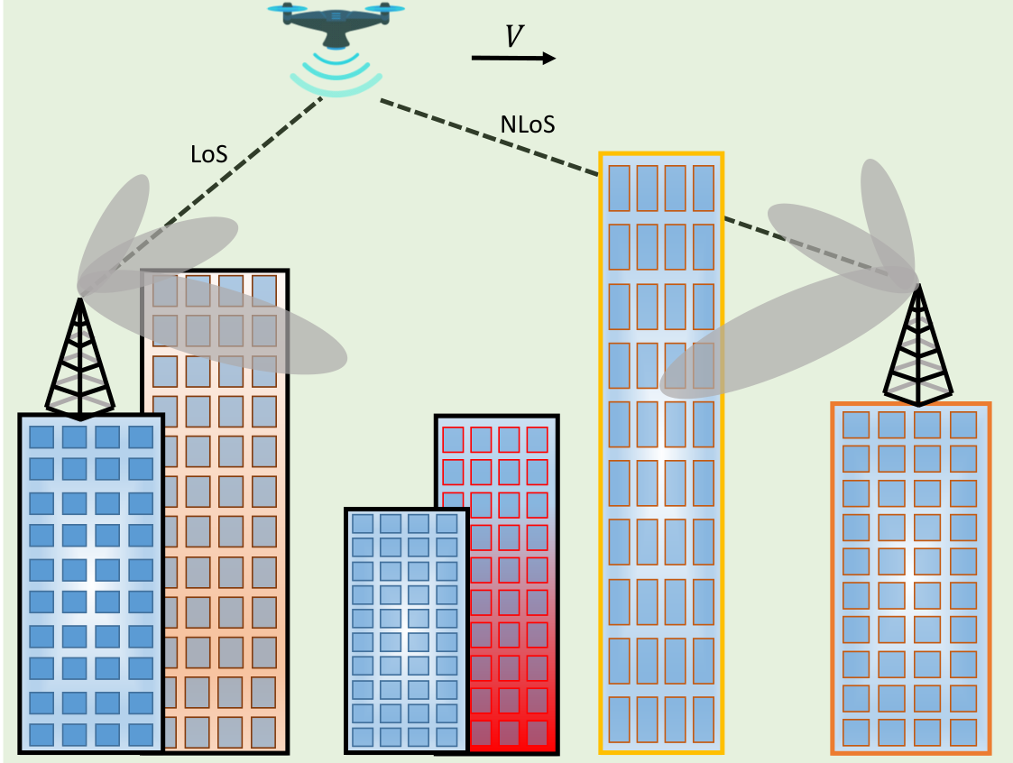
To overcome the above limitations, we propose in this paper a new approach for UAV path design based on reinforcement learning (RL) [9], which is one type of machine learning techniques for solving sequential decision problems. While RL has attracted growing attentions for wireless communications [10] in general and UAV communications in particular [11, 12, 13, 14], to our best knowledge, its application to designing UAV path to avoid the cellular coverage holes (See Fig. 1) has not been reported. To fill the gap, we first formulate an optimization problem to minimize the weighted sum of the UAV’s mission completion time and disconnection duration, and show that the formulated problem can be transformed to a Markov decision process (MDP). An efficient algorithm is then proposed for path design by applying the temporal-difference (TD) method to directly learn the state-value function of the MDP. The algorithm is further extended by using linear function approximation with tile coding so as to deal with large state space. The proposed path design algorithms can be implemented either online, offline, or a combination of both, which only require the raw measured or simulation-generated signal strength as the input. Numerical results show that the proposed path designs can successfully avoid the coverage holes of cellular networks even in the complex urban environment, and significantly outperform the benchmark scheme.
II System Model and Problem Formulation
As shown in Fig. 1, we consider a basic setup of cellular-connected UAV, which aims to design its trajectory from an initial location to a final location with a minimum flying time, while maintaining “good” connectivity with the cellular network. This setup corresponds to many practical UAV applications such as cellular-supported drone delivery, aerial inspection, and data collection. We assume that the UAV flies at a constant altitude and the horizontal coordinates of the initial and final locations are denoted by and , respectively. Let denote the mission completion time and , , represent the UAV trajectory. We then have and . Assume that the feasible region where the UAV can fly is a rectangular area . Define and . We then have , , where denotes element-wise inequality.
Let denote the number of cells that may potentially impact the UAV’s path design, and represent the end-to-end channel coefficient from cell to the UAV, which includes the transmit and receive antenna gains, the large-scale path loss and shadowing, as well as the small-scale fading due to multi-path propagation. As the proposed RL-based path design does not rely on any assumption on the channel modelling, the detailed discussion of one practical BS-UAV channel model is deferred to Section IV. The average received signal power by the UAV from cell , with the average taken over the small scale-fading, is
| (1) |
where is the transmit power of cell . We say that the UAV is disconnected from the cellular network at time if its received signal quality, which is a function of the average received signal powers from the cells, is below a certain threshold , i.e., when . Two typical examples of is the maximum received power, where , and the received signal-to-interference ratio (SIR), where with . Define an indicator function
| (2) |
Then the total UAV disconnection duration can be represented as
| (3) |
It is not difficult to see that is a function of the UAV trajectory , since the average received signal power in (1) depends on via .
Intuitively, with larger mission completion time , the UAV has higher degrees of freedom to design its trajectory to avoid the cellular coverage holes and thus reduce . Our objective is to design to achieve a flexible tradeoff between minimizing and . This can be attained by minimizing the weighted sum of these two metrics with certain weight :
| (4) | ||||
| (5) | ||||
| (6) |
where denotes the maximum UAV speed. It can be shown that at the optimal solution to , the UAV should always fly with the maximum speed , i.e., we have , where with denotes the UAV flying direction. Thus, can be equivalently written as
| (7) | ||||
| (8) | ||||
In practice, designing the UAV path by solving the optimization problems like or faces several challenges, including the need to obtain an accurate and analytically tractable expression for , the requirement of perfect information of the modelling parameters, as well as the difficulty to obtain efficient solutions due to the non-convexity of problems like . In the following, we propose a new approach for UAV path design by leveraging the powerful mathematical framework of RL, which only requires the raw measured or simulation-generated signal strength as the input, without assuming any prior knowledge on the environment.
III Path Design with Reinforcement Learning
III-A An Overview of Reinforcement Learning
This subsection aims to give a very brief overview on RL and settle down the key notations. RL is a useful machine learning framework to solve MDP [9], which consists of an agent and the environment that interact with each other iteratively. With fully observable MDP, at each discrete time step , the agent observes a state , takes an action , and then receives an immediate reward and transits to the next state . Mathematically, a MDP can be specified by 4-tuple , where : the state space; : the action space; : the state transition probability, with specifying the probability of transiting to the next state given the current state after applying the action ; and : the immediate reward received by the agent.
The agent’s actions are governed by its policy , where gives the probability of taking action when in state . The goal of the agent is to improve its policy based on its experience, so as to maximize its long-term expected return , where the return is the accumulated discounted reward from time step onwards with a discount factor .
A key notion of RL is the value function, which includes state-value function and action-value function. The state-value function of a state under policy , denoted as , is the expected return starting from state and following policy thereafter, i.e., . Similarly, the action-value function of taking action at state under policy , denoted as , is the expected return starting from state , taking the action , and following policy thereafter, i.e., . The optimal state-value function, denoted as , is defined as , . Similar definition holds for the optimal action-value function. If the optimal value functions or is known, the optimal policy can be easily obtained either directly or with one-step-ahead search. Thus, the essential task of many RL algorithms is to obtain the optimal value functions, which satisfy the celebrated Bellman optimality equation
Similar Bellman optimality equation holds for the action-value function. Bellman optimality equation is non-linear, where there is no closed-form solution in general. However, many iterative solutions have been proposed, such as model-based dynamic programming (DP) and model-free TD learning. In particular, when the agent has no prior knowledge about the environment of the MDP, it may apply the important idea of TD learning, which is a class of model-free RL methods that learn the value functions based on the direct samples of the state-action-reward-nextState sequence, with the estimation of the value functions updated by the concept of bootstrapping. The simplest TD method makes the following update to the value function with an observed sample [9]
where is the learning rate.
III-B UAV Path Design as an MDP
The first step to apply RL algorithms for solving a real-world problem is to formulate it as an MDP. As MDP is defined over discrete time steps, for the UAV path design problem , we need to first discretize the time horizon into time steps with certain interval . Apparently, should be sufficiently small so that within each time step, the average received signal power by the UAV in (1) remains approximately unchanged. As such, the UAV trajectory can be specified by its discretized representation and . Similarly for the average received signal power in (1), where . As a result, can be re-written as
| (9) | ||||
| (10) | ||||
| (11) | ||||
| (12) |
where (9) is the discrete-time representation of the differential equation (7) with , is the discrete-time counterpart of the indicator function (2), i.e., if and otherwise. Note that we have ignored the constant factor in the objective function of . A natural mapping of to an MDP thus follows:
- •
: the state space constitutes all possible UAV locations within the feasible region, i.e., .
- •
: the action space corresponds to the UAV flying direction, i.e., .
- •
- •
: the reward if the location is covered by the cellular network and otherwise.
With the above MDP formulation, it is observed that the objective function of corresponds to the undiscounted (i.e., ) accumulated rewards over one episode up to time step , i.e., . This corresponds to one particular form of MDP, namely the episodic tasks, which are tasks containing a special state called the terminal state that separates the agent-environment interactions into episodes. After being formulated as a MDP, can be solved by applying various RL algorithms. In the following, we first apply the standard TD learning method to learn the state-value function with state-action discretization, and then extend the algorithm by using linear function approximation with tile coding.
III-C TD Learning with State-Action Discretization
Both the state and action spaces for the MDP defined in Section III-B are continuous. While there are various ways to directly handle continuous state-action MDP problems, the most straightforward approach is to discretize them to form a finite-state MDP. By uniformly discretizing the action space into values, we have , where , with , . With the finite action space and the deterministic state-transition (13), the corresponding discretized state space of can be obtained accordingly, which is denoted as , with representing the total number of discretized states. With such discretizations, the UAV path design problem is quite similar to the gridworld problem [9], but instead of having equal and known rewards, the reward for the studied problem depends on whether the UAV enters a state covered by the cellular network or not.
If the UAV has the perfect knowledge of the MDP, which is the global coverage map for the considered problem, then the standard DP algorithms such as value iteration can be applied to find the optimal UAV path. For scenarios when the UAV has no prior knowledge on the environment, we propose the model-free UAV path design algorithm based on TD learning method, which is summarized in Algorithm 1.
| (14) |
| (15) |
Note that in Algorithm 1, the TD method is applied to learn the state-value function , instead of the action-value function as in the classic Q learning. This is due to the fact that for the studied path design problem, the state-transition is deterministic and known, for which the -greedy policy can be directly obtained from the state-value function via one-step-ahead search, as in (15). This helps reduce the number of variables from to . In Algorithm 1, the learning rate and the exploration parameter decrease with the episode number as in Step 4, which encourages learning and exploration at early stages while promoting exploitation as gets sufficiently large.
While theoretically, the convergence of Algorithm 1 is guaranteed for any initialization of the state-value function [9], in practice, a random or all-zero initialization of may require infinite time steps for the UAV to reach the destination . Intuitively, should be initialized in a way such that in the first episode when the UAV has completely no knowledge about the radio environment, a reasonable trial should be selecting actions for the shortest path flying. Thus, we propose the distance-based value function initialization for Algorithm 1, with , .
III-D TD Learning with Tile Coding
The TD learning method in Algorithm 1 is known as table-based, which requires storing and updating values, each for one state, and the state value is updated only when that state is actually visited. This becomes impractical for continuous state or when the number of discretized states is large. In order to practically apply many RL algorithms, one may resort to the useful technique of function approximation [9], where the state-value function is approximated by certain parametric function , , with a parameter vector . Function approximation brings two advantages over table-based RL. Firstly, instead of storing and updating the value functions for all states, one only needs to learn the parameter , which typically has lower dimension than the number of states, i.e., . Secondly, function approximation enables generalization, i.e., the ability to predict the state-values even for those states that have never been visited, since different states are coupled with each other. A common metric for updating is mean squared error (MSE), where .
The simplest function approximation is linear approximation, where , with referred to as the feature vector of state . With linear function approximation, for each state-reward-nextState transition observed by the agent, can be updated to minimize based on the stochastic semi-gradient method [9]. For the TD method with one-step bootstrapping, we have
| (16) |
where determines the learning rate.
The remaining task is to construct the feature vector . In this paper, we propose to use tile coding [9] for feature vector construction for UAV path design. Tile coding can be regarded as a more general form of state space discretization. For the 2D rectangular area , instead of directly discretizing it into non-overlapping grids with sufficiently small grid size as in Section III-C, with tile coding, it is partitioned into grids with larger size, but there are many such partitions that are offset from one another by a uniform amount in each dimension. Each such partition is called a tiling and each element of the partition is called a tile. Fig. 2 gives an illustration with 3 tilings, each having 12 tiles.
As shown in Fig. 2, let and denote the length and width of the rectangular area, respectively, denote the number of tilings, and denote the size of each tile. Then the offset between adjacent tilings can be shown to be and along the x- and y- dimensions, respectively. Let denote the number of tiles for each tiling. Then should be large enough to cover the length even after offset. Based on Fig. 2, we have , or . Similar relationship can be obtained for . Thus, the number of tiles for each tiling is , and the total number of tiles with all tilings is . It is not difficult to see that while tiles of the same tiling are non-overlapping, those from different tilings may overlap with each other. This renders it possible to represent each point in the space by specifying the active tile of each tiling, which requires exactly variables. However, an effective way of representation is to use a binary vector of dimension , with each element corresponding to one tile resulting from the tilings. is a sparse vector with most elements being except for the elements corresponding to the active tiles in each tiling. This gives the feature vector of linear function approximation with tile coding.
The pseudo-code of TD learning with tile coding is quite similar to Algorithm 1, with the following straightforward modifications: (i) Replace the state-value function by , if , and for ; (ii) Replace the value function update in Step 10 of Algorithm 1 with the parameter update (16). Besides, to have the same learning rate as in Algorith 1, the parameter in (16) should be set as ; iii) Different from Table-based update in Algorithm 1, function approximation may result in very close estimated state values for adjacent states. This may result in cyclic path with the -greedy action (15) between adjacent states like , which is obviously undesired. A simple remedy to this is to keep a copy of the previous state , and (15) is slightly revised by excluding the action that would lead to ; iv) Similar to Algorithm 1, the parameter should be initialized so as to encourage the shortest-path flying at the first episode. To this end, is initialized to the least square solution by minimizing , where is a selected subset of the state space to initialize , is the matrix with the feature vectors , as the columns, and is the vector with the distances to as the elements.
IV Numerical Results
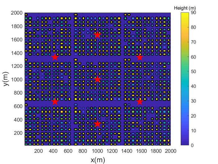
Numerical results are provided to evaluate the performance of the proposed UAV path designs. As shown in Fig. 3, we consider an urban area of size 2 km 2 km with high-rise buildings, which constitute the most challenging environment for communication-aware UAV path design, since the LoS/NLoS links and the received signal strength may alter frequently as the UAV flies (see Fig. 1). To accurately simulate the BS-UAV channels, we first generate the building locations and height based on one realization of the statistical model suggested by the International Telecommunication Union (ITU) [15], which involves three parameters: : the ratio of land area covered by buildings to the total land area; : the mean number of buildings per unit area; and a variable determining the building height distribution, which is usually modelled as Rayleigh with mean . Fig. 3 shows the realization of the building locations and height with , buildings/km2, and m. For simplicity, all building height is clipped to below m.
We assume a hexagonal cell layout with two tiers in the considered area, which corresponds to 7 BS sites with locations marked by red stars in Fig. 3, and the BS antenna height is m [4]. With the standard sectorization technique, each BS site contains 3 sectors/cells. Thus, the total number of cells is . The BS antenna model follows the 3GPP specification [16], where an 8-element uniform linear array (ULA) is placed vertically with pre-determined phase shift to electrically downtilt the main lobe by . This leads to the directional antenna with fixed 3D radiation pattern, which is shown in Fig. 4 of [1]. To obtain the average signals received by the UAV from each cell, at each possible UAV location, we firstly determine whether there exists a LoS link between the UAV and the BS according to the building information, and then use the 3GPP BS-UAV path loss model for urban Macro (UMa) given in Table B-2 of [4].
We assume that the UAV’s flying altitude is m, and the SIR defined in Section II is used as the performance measure to determine the cellular connectivity by the UAV. Fig. 4 shows the global coverage map with dBm and dB, together with the resulting UAV paths from the initial location m to the final location m with four schemes: i) the direct path from to ; ii) the value-iteration based DP, which requires the perfect global coverage map; iii) the TD learning method proposed in Section III-C; and iv) TD learning with tile coding proposed in Section III-D. The following parameters are used: , , m, , , and . For tile coding, the number of tilings is , and each tile has size m m. It is observed from Fig. 4 that except the benchmark direct flight, the other three schemes all successfully find UAV paths that avoid the coverage holes of the cellular network. Furthermore, the table-based TD learning scheme gives a similar path as the optimal DP scheme. It is also noted that for TD with tile coding, a more conservative path with longer flying distance is obtained, since with linear function approximation, it seems more challenging to discover the narrow “bridge” as taken by the other two methods.

Fig. 5 shows the accumulated reward per episode for the TD learning algorithms. It is observed that both TD learning methods converge to values very close to the optimal DP solution, which significantly outperform the benchmark direct flight. It is also observed that tile coding helps improve the convergence speed of the TD learning method, though it eventually gives slightly worse performance. Lastly, it is observed that both TD learning methods require thousands of episodes to converge. This gives rise to the typical issue of RL, i.e., learning from real experience is usually sample expensive. Fortunately, such issue can be alleviated by firstly pre-training the policy with simulation-generated samples according to certain (even inaccurate) communication model, which is almost cost-free, and then further refine the policy by actual UAV flight with online learning to address the model inaccuracy issue.
V Conclusions
This paper studies path designs for cellular-connected UAVs. To overcome the limitations of conventional optimization-based path design approaches, we propose RL-based algorithms, which only require the measured or simulation-generated raw signal strength as the input and are suitable for both online and offline implementations. The proposed algorithm utilizes the TD method to learn the state-value function, and it is further extended by applying linear function approximation with tile coding. Numerical results are provided to show the effectiveness of the proposed algorithms.
References
- [1] Y. Zeng, Q. Wu, and R. Zhang, “Accessing from the sky: a tutorial on UAV communications for 5G and beyond,” submitted to Proceedings of the IEEE, available online at arXiv/1903.05289.
- [2] Y. Zeng, R. Zhang, and T. J. Lim, “Wireless communications with unmanned aerial vehicles: opportunities and challenges,” IEEE Commun. Mag., vol. 54, no. 5, pp. 36–42, May 2016.
- [3] Qualcomm, “LTE unmanned aircraft systems,” trial Report, available online at https://www.qualcomm.com/documents/lte-unmanned-aircraft-systems-trial-report, May, 2017.
- [4] 3GPP TR 36.777: “Technical specification group radio access network: study on enhanced LTE support for aerial vehicles”, V15.0.0, Dec., 2017.
- [5] Y. Zeng, J. Lyu, and R. Zhang, “Cellular-connected UAV: potentials, challenges and promising technologies,” IEEE Wireless Commun., vol. 26, no. 1, pp. 120–127, Feb. 2019.
- [6] S. Zhang, Y. Zeng, and R. Zhang, “Cellular-enabled UAV communication: a connectivity-constrained trajectory optimization perspective,” IEEE Trans. Commun., vol. 67, no. 3, pp. 2580–2604, Mar. 2019.
- [7] E. Bulut and I. Guvenc, “Trajectory optimization for cellular-connected UAVs with disconnectivity constraint,” in Proc. IEEE International Conference on Communications (ICC), May 2018.
- [8] Y. Zeng and R. Zhang, “Energy-efficient UAV communication with trajectory optimization,” IEEE Trans. Wireless Commun., vol. 16, no. 6, pp. 3747–3760, Jun. 2017.
- [9] R. S. Sutton and A. G. Barto, Reinforcement learning: An introduction, 2nd ed. MIT Press, Cambridge, MA, 2018.
- [10] C. Jiang, et al., “Machine learning paradigms for next-generation wireless networks,” IEEE Wireless Commun., vol. 24, no. 2, pp. 98–105, Apr. 2017.
- [11] H. Bayerlein, P. Kerret, and D. Gesbert, “Trajectory optimization for autonomous flying base station via reinforcement learning,” in SPAWC, Jun. 2018.
- [12] X. Liu, Y. Liu, and Y. Chen, “Deployment and movement for multiple aerial base stations by reinforcement learning,” in IEEE Global Communications Conference (GLOBECOM), 2018.
- [13] H. Bayerlein, R. Gangula, D. Gesbert, “Learning to rest: A Q-learning approach to flying base station trajectory design with landing spots,” in Proc. Asilomar Conf. on Signals, Systems, and Computers, Oct. 2018.
- [14] U. Challita, W. Saad, and C. Bettstetter, “Interference management for cellular-connected UAVs: A deep reinforcement learning approach,” IEEE Trans. Wireless Commun., vol. 18, no. 4, pp. 2125–2140, Apr. 2019.
- [15] ITU-R, Rec. P.1410-5 “Propagation Data and Prediction Methods required for The Design of Terrestrial Broadband radio Access systems operating in a frequency range from 3 to 60 GHz”,P Series, Radiowave propagation, Feb. 2012.
- [16] 3GPP TR 36.873: “Study on 3D channel model for LTE”, V12.7.0, Dec., 2017.