An N2HDM Solution for the possible 96 GeV Excess
Abstract:
We discuss a signal (local) in the light Higgs-boson search in the diphoton decay mode at as reported by CMS, together with a excess (local) in the final state at LEP in the same mass range. We review the interpretation of this possible signal as a Higgs boson in the 2 Higgs Doublet Model with an additional real Higgs singlet (N2HDM). It is shown that the lightest Higgs boson of the N2HDM can perfectly fit both excesses simultaneously, while the full Higgs-boson sector is in agreement with all Higgs-boson measurements and exclusion bounds as well as other theoretical and experimental constraints. It is demonstrated that in particular the N2HDM type II and can fit the data best, leading to a supersymmetric interpretation. The NMSSM and the are briefly reviewed in this respect.
(CORFU2018)
31 August - 28 September, 2018
Corfu, Greece
1 Introduction
The Higgs boson discovered in 2012 by ATLAS and CMS [1, 2] – within theoretical and experimental uncertainties – is consistent with the existence of a Standard-Model (SM) Higgs boson [3]. However, the measurements of Higgs-boson couplings, which are known experimentally to a precision of roughly , leave room for Beyond Standard-Model (BSM) interpretations. Many BSM models possess extended Higgs-boson sectors. which naturally contain additional Higgs bosons with masses larger than . However, many extensions also offer the possibilty of additional Higgs bosons below . Consequently, the search for lighter Higgs bosons forms an important part in the BSM Higgs-boson analyses.
Searches for Higgs bosons below have been performed at LEP, the Tevatron and the LHC. LEP reported a local excess observed in the searches [4], which would be consistent with a scalar of mass , but due to the final state the mass resolution is rather coarse). The excess corresponds to
| (1) |
where the signal strength is the measured cross section normalized to the SM expectation, with the SM Higgs-boson mass at . The value for was extracted in Ref. [5] using methods described in Ref. [6].
Recent CMS Run II results [7] for Higgs-boson searches in the diphoton final state show a local excess of around , with a similar excess of in the Run I data at a comparable mass [8]. The excess corresponds to (combining 7, 8 and data, and assuming that the production dominates)
| (2) |
First Run II results from ATLAS with fb-1 in the searches below GeV turned out to be weaker than the corresponding CMS results, see, e.g., Fig. 1 in Ref. [9].
Reviews about the possibility that these two excesses, found effectively at the same mass, are of a common origin. are given in Refs. [10, 9]. The list comprises of type I 2HDMs [11, 12], a radion model [13], a minimal dilaton model [14], as well as supersymmetric models [15, 16, 17].
Motivated by the Hierarchy Problem, Supersymmetry (SUSY) plays a prominent role in BSM physics. The simplest SUSY extension of the SM is the Minimal Supersymmetric Standard Model (MSSM) [18, 19], doubling the degrees of freedom of the SM supplemented with a second Higgs doublet. The MSSM Higgs sector, composed of and , consists of two -even, one -odd and two charged Higgs bosons. The light (or the heavy) -even MSSM Higgs boson can be interpreted as the signal discovered at [20] (see Refs. [21, 22] for recent updates). However, in Ref. [21] it was demonstrated that the MSSM cannot explain the CMS excess in the diphoton final state. This can be traced back to the “too rigid” structure of the 2HDM (type II) strucure of the Higgs-boson sector in the MSSM.
This raises the question whether simple extensions of the 2HDM can fit both the CMS excess in Eq. (2) and the LEP exceses in Eq. (1). In Ref. [23] the Next to minimal 2 Higgs doublet model (N2HDM) [24, 25] was investigated. In this model the two Higgs doublets are supplemented with a real Higgs singlet, giving rise to one additional (potentially light) -even Higgs boson. However, in comparison to SUSY models the N2HDM does not have to obey the SUSY relations in the Higgs-boson sector. Consequently, it allows to study how the potential fits the two excesses simultaneously in a more general way. Here we review first the results obtained in the N2HDM [23] and then two possible SUSY realizations.
2 The N2HDM, constraints and the experimental excesses
2.1 The N2HDM
The N2HDM is the simplest extension of a -conserving two Higgs doublet model (2HDM) in which the latter is augmented with a real scalar singlet Higgs field, denoted as , and , respectively (see, e.g., Refs. [24, 25]). As in the 2HDM a symmetry is imposed to avoid flavor changing neutral currents at the tree-level, only softly broken in the Higgs sector via the bilinear mass term . As in the 2HDM, this leads to four variants of the N2HDM, depending on the parities of the fermions. Taking the electroweak symmetry breaking (EWSB) minima to be charge and -conserving, the scalar fields after EWSB can be parametrised as
where are the real vevs acquired by the fields and respectively. As in the 2HDM we define . The -even Higgs-boson sector contains three physical Higgses. Thus, a rotation from the interaction to the physical basis can be achieved with the help of a orthogonal matrix as
with . The rotation matrix can be parametrized as
| (15) |
being the three mixing angles, and we use the short-hand notation , . The couplings of the Higgs bosons to SM particles are modified w.r.t. the SM Higgs-coupling predictions due to the mixing in the Higgs sector. It is convenient to express the couplings of the scalar mass eigenstates normalized to the corresponding SM couplings. We therefore introduce the coupling coefficients and , such that the couplings to the massive vector bosons are given by
| (16) |
where is the gauge coupling, the cosine of weak mixing angle, , and and the masses of the boson and the boson, respectively. The couplings of the Higgs bosons to the SM fermions are given by
| (17) |
where is the mass of the fermion and is the SM vev. The coupling coefficients for the couplings to gauge bosons for the three -even Higgses. are identical in all four types of the (N)2HDM. They differ, however, as in the 2HDM depending on the type of the model, as summarized in Tab. 1.
| -type () | -type () | leptons () | |
|---|---|---|---|
| type I | |||
| type II | |||
| type III (lepton-specific) | |||
| type IV (flipped) |
There are 12 independent parameters in the model, which can be taken as [25];
| (18) |
where , denote the masses of the physical -odd and charged Higgses respectively.
In Ref. [23] the code ScannerS [26, 25] has been used to uniformly explore the set of independent parameters as given in Eq. (18) (see below). The lightest -even Higgs boson, , was identified with the one being potentially responsible for the signal at . The second lightest -even Higgs boson was identified with the one observed at .
2.2 Constraints
All relevant constraints on the N2HDM were taken into account, see Ref. [23] for more details. These comprise
- •
Theoretical constraints:
tree-level perturbativity and the condition that the vacuum should be a global minimum of the potential. - •
- •
Constraints from the SM-like Higgs-boson properties:
Any model beyond the SM has to accommodate the SM-like Higgs boson, with mass and signal strengths as they were measured at the LHC. In our scans the compatibility of the -even scalar with a mass of with the measurements of signal strengths at Tevatron and LHC is checked with the code HiggsSignals v.2.2.3 [32, 33, 34]. The corresponding theory predictions are proved by a combination of the codes ScannerS, SusHi [35, 36] and N2HDECAY [25, 37, 38]. The HiggsSignals output shown below consists in the reduced ,(19) where is provided by HiggsSignals and is the number of experimental observations considered.
- •
Constraints from flavor physics:
In the low region that is of interest (see below) the constraints which must be taken into account are [39]: , constraints on from neutral meson mixing and . Constraints from excludes for all values of in the type II and IV 2HDM, while for type I and III the bounds are more dependent. - •
Constraints from electroweak precision data:
Constraints from electroweak precision observables can in a simple approximation be expressed in terms of the oblique parameters S, T and U [40, 41]. Deviations to these parameters are significant if new physics beyond the SM enters mainly through gauge boson self-energies, as it is the case for extended Higgs sectors. These constraints are implemented in ScannerS. For points to be in agreement with the experimental observation, it was required that the prediction of the and the parameter are within the ellipse, corresponding to for two degrees of freedom.
2.3 Experimental excesses
As experimental input for the signal strengths in Ref. [23] the values
| (20) |
The evaluation of the signal strengths for the excesses was done in the narrow width approximation. For the LEP excess this is given by,
| (21) |
evaluated with the help of N2HDECAY. For the CMS signal strength one finds,
| (22) |
The SM predictions for the branching ratios and the cross section via ggF can be found in Ref. [44].
| Decrease | No decrease | No enhancement | |
|---|---|---|---|
| type I | ✓ | ✗ | ✓ |
| type II | ✓ | ✓ | ✓ |
| lepton-specific | ✓ | ✗ | ✗ |
| flipped | ✓ | ✓ | ✗ |
As can be seen from Eqs. (20) - (22), the CMS excess points towards the existence of a scalar with a SM-like production rate, whereas the LEP excess demands that the scalar should have a squared coupling to massive vector bosons of times that of the SM Higgs boson of the same mass. This suppression of the coupling coefficient is naturally fulfilled for a singlet-like state, that acquires its interaction to SM particles via a considerable mixing with the SM-like Higgs boson, thus motivating the explanation of the LEP excess with the real singlet of the N2HDM. For the CMS excess, on the other hand, it appears to be difficult at first sight to accommodate the large signal strength, because one expects a suppression of the loop-induced coupling to photons of the same order as the one of , since in the SM the Higgs-boson decay to photons is dominated by the boson loop. However, it turns out that it is possible to overcompensate the suppression of the loop-induced coupling to photons by decreasing the total width of the singlet-like scalar, leading to an enhancement of the branching ratio of the new scalar to the final state. The different types of N2HDM behave differently in this regard, based on how the doublet fields are coupled to the quarks and leptons. The general idea is summarized in Tab. 2.
In Ref. [23] it was argued that only the type II and type IV (flipped) N2HDM can accommodate both excesses simultaneously using a dominantly singlet-like scalar at . The first condition is that the coupling of to -quarks has to be suppressed to enhance the decay rate to , as the total decay width at this mass is still dominated by the decay to . At the same time one can not decrease the coupling to -quarks too much, because the decay width to photons strongly depends on the top quark loop contribution (interfering constructively with the charged Higgs contribution). Moreover, the ggF production cross section is dominated at leading order by the diagram with -quarks in the loop. Thus, a decreased coupling of to -quarks implies a lower production cross section at the LHC. As one can deduce from Tab. 2, in type I and type III of the N2HDM, the coupling coefficients are the same for up- and down-type quarks. Thus, it is impossible to satisfy both of the above criteria simultaneously in these models. Consequently, they fail to accommodate both the CMS and the LEP excesses and are discarded from now on.
In Ref. [23] it is furthermore concluded that in type II and IV that corresponds to an enhancement of the branching ratio to photons, because the dominant decay width to -quarks, and therefore the total width of , is suppressed.
A third condition, although not as significant as the other two, is related to the coupling of to leptons. If it is increased, the decay to a pair of -leptons will be enhanced. Similar to the decay to -quarks, it will compete with the diphoton decay and can suppress the signal strength needed for the CMS excess. The -Yukawa coupling is not as large as the -Yukawa coupling, so this condition is not as important as the other two. Still, as will be reviewed below, it is the reason why it is easier to fit the CMS excess in the type II model compared to the flipped scenario.
In the scans we indicate the “best-fit point” referring to the point with the smallest defined by
| (23) |
quantifying the quadratic deviation w.r.t. the measured values, assuming that there is no correlation between the signal strengths of the two excesses.
3 Results
In the following we will describe the analysis in the type II (with similar results in type IV [23]). The scalar mass eigenstate with dominant singlet-component will be responsible for accommodating the LEP and the CMS excesses at -. The second lightest Higgs-boson will be placed at with the requirement that it behaves within the uncertainties as the SM Higgs-boson. Similar scans have been performed also for the N2HDM type I and III (lepton specific), confirming that these types cannot fit well the two excesses.
The following ranges of input parameters have been scanned:
| (24) |
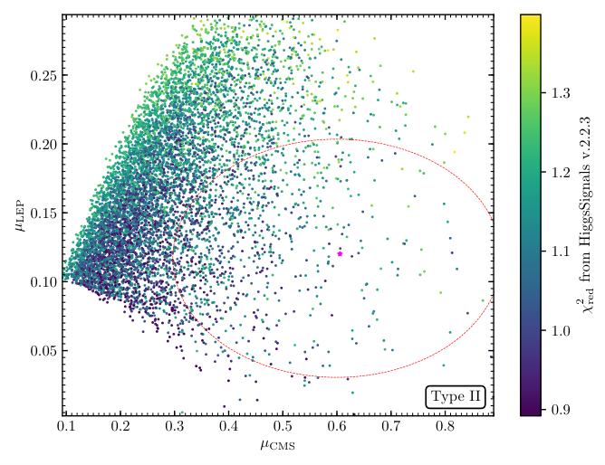
We show the result of the scan in Fig. 1 [23] in the plane of the signal strengths and for each scan point, where the best-fit point w.r.t. the two excesses is marked by a magenta star. It should be kept in mind that the density of points has no physical meaning and is a pure artefact of the “flat prior” in our parameter scan. The red dashed line corresponds to the ellipse, i.e., to for two degrees of freedom, with defined in Eq. (23). The colors of the points indicate the reduced from the test of the SM-like Higgs-boson properties with HiggsSignals. One sees that various points fit both excesses simultaneously while also accommodating the properties of the SM-like Higgs boson at . The lowest (hightest) value of in the ellipse is , whereas the the lowest (highest) value of is found to be 0.797 (3.748). It should be emphasized that the dependence of the branching ratio of to diphotons, and therefore of , on is due to the positive correlation between and the total decay width of . The additional contributions to the diphoton decay width of diagrams with the charged Higgs boson in the loop has a minor dependence on for .
In Tab. 3 we review the values of the free parameters and the relevant branching ratios of the neutral scalars for the best-fit point of our scan, which is highlighted with a magenta star in Figs. 1. Remarkably, the branching ratio for the singlet-like scalar to photons is larger than the one of the SM-like Higgs boson. As explained in the beginning of Sect. 3 this is achieved by a value of , which suppresses the decay to -quarks and -leptons, without decreasing the coupling to -quarks. Constraints from the oblique parameters lead to a -odd Higgs-boson mass or a heavy -even Higgs-boson mass close to the mass of the charged Higgs boson.
4 Future searches
4.1 Indirect searches


Currently, uncertainties on the measurement of the coupling strengths of the SM-like Higgs boson at the LHC are still large, i.e., at the -level they are of the same order as the modifications of the couplings present in our analysis in the N2HDM [3, 48, 47]. In the future, once the complete collected at the LHC are analyzed, the constraints on the couplings of the SM-like Higgs boson will benefit from the reduction of statistical uncertainties. Even tighter constraints are expected from the LHC after the high-luminosity upgrade (HL-LHC), when the planned amount of integrated luminosity will have been collected [49]. Finally, a future linear collider like the ILC, CLIC, FCC-ee or CepC could improve the precision measurements of the Higgs-boson couplings even further [49, 50], where we will use ILC numbers for illustration. At an collider the cross section of the Higgs boson can be measured independently, and the total width (and therefore also the coupling modifiers) can be reconstructed without model assumptions.
Several studies have been performed to estimate the future constraints on the coupling modifiers of the SM-like Higgs boson at the LHC [49, 51, 52, 53, 54] and the ILC [49, 55, 56, 57, 58, 46, 45], assuming that no deviations from the SM predictions will be found. Here, we review the comparison of the scan points to the expected precisions of the HL-LHC and the ILC as they are reported in Refs. [46, 45], neglecting possible correlations of the coupling modifiers. The results are shown in Fig. 2 [23].
We plot the effective coupling coefficient of the SM-like Higgs boson to -leptons on the horizontal axis against the coupling coefficient to -quarks (top) and to -quarks (bottom) for both types. These points passed all the experimental and theoretical constraints, including the verification of SM-like Higgs-boson properties in agreement with LHC results using HiggsSignals. In the top plot the blue points lie on a diagonal line, because in type II the coupling to leptons and to down-type quarks scale identically, while in the bottom plot the red points representing the type IV scenario lie on the diagonal, because there the lepton-coupling scales in the same way as the coupling to up-type quarks.
In Fig. 2 the current measurements on the coupling modifiers by ATLAS [48] and CMS [47] are shown as black ellipses. The magenta ellipse in each plot shows the expected precision of the measurement of the coupling coefficients at the -level at the HL-LHC from Ref. [45]. The current uncertainties and the HL-LHC analysis are based on the coupling modifier, or -framework, in which the tree-level couplings of the SM-like Higgs boson to vector bosons, the top quark, the bottom quark, the and the lepton, and the three loop-induced couplings to , and receive a factor quantifying potential modifications from the SM predictions. These modifiers are then constrained using a global fit to projected HL-LHC data assuming no deviation from the SM prediction will be found. The uncertainties found for the can directly be applied to the future precision of the coupling modifiers we use in our paper. We use the uncertainties given under the assumptions that no decay of the SM-like Higgs boson to BSM particles is present, and that current systematic uncertainties will be reduced in addition to the reduction of statistical uncertainties due to the increased statistics.
The green and the orange ellipses show the corresponding expected uncertainties when the HL-LHC results are combined with projected data from the ILC after the phase and the phase, respectively, taken from Ref. [46]. Their analysis is based on a pure effective field theory calculation, supplemented by further assumptions to facilitate the combination with the HL-LHC projections in the -framework. In particular, in the effective field theory approach the vector boson couplings can be modified beyond a simple rescaling. This possibility was excluded by recasting the fit setting two parameters related to the couplings to the -boson and the -boson to zero (for details we refer to Ref. [46]).
Remarkably, the expected constraints from the HL-LHC and the ILC will strongly reduce the allowed parameter spaces and allow a clear test of the models under consideration. Independent of the type of the N2HDM, we can see comparing both plots in Fig. 2, that there is not a single scan point that coincides with the SM prediction regarding the three coupling coefficients shown. This implies that, once these couplings are measured precisely by the HL-LHC and the ILC, a deviation of the SM prediction has to be measured in at least one of the couplings, if our explanation of the excesses is correct. Accordingly, if no deviation from the SM prediction regarding these couplings will be measured, our explanation would be ruled out entirely.
Furthermore, in case a deviation from the SM prediction will be found, the predicted scaling behavior of the coupling coefficients in the type II scenario (upper plot) and the type IV scenario (lower plot), might lead to distinct possibilities for the two models to accommodate these possible deviations. In this case, precision measurements of the SM-like Higgs boson couplings could be used to exclude one of the two scenarios. This is true for all points except the ones highlighted in yellow in Fig. 2. The yellow points are a subset of points of our scans that, if such deviations of the SM-like Higgs boson couplings will be measured, could correspond to a benchmark point of both the scan in the type II and the type IV scenario. However, note that this subset of points is confined to the diagonal lines of both plots, and thus corresponds to a very specific subset of the overall allowed parameter space. For the type II scenario, in the upper plot, the yellow points are determined by the additional constraint that , which is exactly true in the type IV scenario. For the type IV scenario, in the lower plot, the yellow points are determined by the additional constraint that , which is exactly true in the type II scenario.

For completeness we show in Fig. 3 the absolute value of the coupling modifier of the SM-like Higgs boson w.r.t. the vector boson couplings on the vertical axis. Again, the parameter points of both types show deviations larger than the projected experimental uncertainty at HL-LHC and ILC. The deviations in are even stronger than for the couplings to fermions. A deviation from the SM prediction is expected with HL-LHC accuracy. At the ILC a deviation fo more than would be visible. As mentioned already, a suppression of the coupling to vector bosons is explicitly expected by demanding . However, since points with lower singlet component cannot accommodate both excesses, this does not contradict the conclusion that the explanation of both excesses can be probed with high significance with future Higgs-boson coupling measurements.
4.2 Direct searches
To start with, the diphoton bump which has persisted through LHC Run I and II is worth exploring in additional Higgs boson searches of future runs of the LHC. Furthermore, the search for charged Higgs bosons appears promising in the region of low . Searches at the (HL-)LHC will yield strong constraints or (hopefully) discover signs of a charged Higgs-boson in the region between and . Prospects for a discovery in the charged Higgs-boson searches in the decay mode can be found in Ref. [59].
Since the charged Higgs boson is rather heavy due to the constraints from flavor physics, exotic signals at colliders can be expected from the decay of the charged Higgs boson into a boson and a neutral Higgs bosons. We show the corresponding branching ratios in Fig. 4, 5 and 6 for the decays of into and , and , respectively. The blue points are the ones that lie inside the ellipse of and . The decays into the two light Higgs bosons is always kinematically allowed. However, as one can see in Fig. 6, if the decay to the heavy Higgs boson opens up kinematically, it is usually the dominant of the three, and competes with ordinary decay modes of into a pair of quarks. The smallest branching ratio for the mass range of in our scan is the one to the SM-like Higgs boson , which is minimized in the limit of becoming SM-like. Concerning the decay to the lightest Higgs boson , a correlation is visible. The points explaining both excesses within the uncertainty have larger branching fractions. In order for this decay to happen, needs a sizable doublet component, otherwise it would not couple to the boson. The doublet component is, as explained before, also necessary for to contribute to the signal strengths at LEP and CMS.
The prospects for the searches for the heavy neutral Higgs bosons, decaying dominantly to , may also be promising. However, we are not aware of corresponding HL-LHC projections.
colliders, on the other hand show good prospects for the search of light scalars [60, 50]. The main production channel in the mass and energy range that we are interested in is the Higgs-strahlung process , where is the scalar being searched for. The LEP collaboration has previously performed such searches [4], which resulted in the excess given by . These searches were limited by the low luminosity of LEP. However, the ILC, with its much higher luminosity and the possibility of using polarized beams, has a substantially higher potential to discover the light scalars. The searches performed at LEP can be divided into two categories: the ’traditional method’, where studies are based on the decay mode along with decays to final states. This method introduces certain amount of model dependence into the analysis because of the reference to a specific decay mode of . The more model independent ’recoil technique’ used by the OPAL collaboration of LEP looked for light states by analyzing the recoil mass distribution of the di-muon system produced in decay [61].
In Fig. 7 [23] the bounds from the LEP as well as the projected bounds from the ILC searches for light scalars in type II N2HDM scenarios are shown. The lines indicating the ILC reach for a machine with beam polarizations of and an integrated luminosity of 2000 are as evaluated in Ref. [50]. The quantity used in their analysis corresponds to an upper limit at the confidence level on the cross section times branching ratio generated within the ’background only’ hypothesis, where the cross section has been normalized to the reference SM-Higgs cross section and the BRs have been assumed to be as in the SM (with a Higgs boson of the same mass). Consequently, we take the obtained limits to be valid for the total cross section times branching ratio. The colored points shown in Fig. 7 are the points of the scans in the type II scenario satisfying all the theoretical and experimental constraints. The plot show that the parameter points of the scans can completely be covered by searches at the ILC for additional Higgs-like scalars. Depending on , i.e., the light Higgs-boson production cross section, the can be produced and analyzed in detail at the ILC.
5 Supersymmetric realizations
In Sect. 2.3 it was demonstrated that due to the structure of the couplings of the Higgs doublets to fermions only two types of the N2HDM, type II and type IV (flipped), can fit simultaneously the two excesses. Due to the different coupling to leptons in type II and type IV, in general larger values of can be reached in the former, and the CMS excess can be fitted “more naturally” in the type II N2HDM. Incidentally, this is exactly the Higgs sector that is required by supersymmetric models. On the other hand, in Ref. [21] it was shown that the MSSM cannot explain the CMS excess in the diphoton final state. This can be traced back to the “too rigid” structure of the 2HDM (type II) strucure of the Higgs-boson sector in the MSSM. SUSY models that can potentially explain both excesses simultaneously, consequently, should contain (at least) an additional Higgs singlet.
Going beyond the MSSM, a well-motivated extension is given by the Next-to-MSSM (NMSSM), see [62, 63] for reviews. In the NMSSM a new singlet superfield is introduced, which only couples to the Higgs- and sfermion-sectors, giving rise to an effective -term. In the -conserving case the NMSSM Higgs sector consists of three -even Higgs bosons, (), two -odd Higgs bosons, (), and the charged Higgs boson pair . In the NMSSM not only the lightest but also the second lightest -even Higgs boson can be interpreted as the signal observed at about , see, e.g., [64, 65]. In Ref. [16] it was demonstrated that the NMSSM can indeed simultaeneously satisfy the two excesses mentioned above. In this case, the Higgs boson at has a large singlet component, but also a sufficiently large doublet component to give rise to the two excesses.
A natural extension of the NMSSM is the , in which the singlet superfield is interpreted as a right-handed neutrino superfield [66, 67], see Refs. [68, 69, 70] for reviews. The is the simplest extension of the MSSM that can provide massive neutrinos through a see-saw mechanism at the electroweak scale. A Yukawa coupling for right-handed neutrinos of the order of the electron Yukawa coupling is introduced that induces the explicit breaking of -parity. Also in the the signal at can be interpreted as the lightest or the second lightest -even scalar. In Ref. [15] the “one generation case” (only one generation of massive neutrinos) was analyzed. In this case Higgs-boson sector of the effectively resembles the Higgs-boson sector in the NMSSM. In Ref. [15] it was found that also the can fit the CMS and the LEP excesses simultaneously. In this case the scalar at has a large right-handed sneutrino component. The three generation case (i.e. with three generations of massive neutrinos) is currently under investigation [71].
6 Conclusions
A excess (local) in the diphoton decay mode at was reported by CMS, as well as a excess (local) in the final state at LEP in the same mass range. We reviewed the interpretation this possible signal as a Higgs boson in the 2 Higgs Doublet Model with an additional real Higgs singlet (N2HDM) [23].
All relevant constraints were included in the analysis. These are theoretical constraints from perturbativity and the requirement that the minimum of the Higgs potential is a global minimum. We take into account the direct searches for additional Higgs bosons from LEP. the Tevatron and the LHC, as well as the measurements of the properties of the Higgs boson at . We furthermore include bounds from flavor physics and from electroweak precision data.
It was demonstrated that due to the structure of the couplings of the Higgs doublets to fermions only two types of the N2HDM, type II and type IV (flipped), can fit simultaneously the two excesses. On the other hand, the other two types, type I and type III (lepton specific), cannot be brought in agreement with the two excesses. Subsequently, the free parameters in the two favored versions of the N2HDM were scanned, where the results are similar in both scenarios. It was found that the lowest possible values of above and just above 1 are favored. The reduced from the Higgs-boson measurements is found roughly in the range . Due to the different coupling to leptons in type II and type IV, in general larger values of can be reached in the former, and the CMS excess can be fitted “more naturally” in the type II N2HDM. Incidentally, this is exactly the Higgs sector that is required by supersymmetric models.
It was analyzed how the favored scenarios can be tested at future colliders. The (HL-)LHC will continue the searches/measurements in the diphoton final state. But apart from that we are not aware of other channels for the light Higgs boson that could be accessible. Concerning the searches for heavy N2HDM Higgs bosons, particularly interesting are the prospects for charged Higgs bosons. For the low values favored in our analysis, these searches have the best potential to discover a new heavy Higgs boson at the LHC Run III or the HL-LHC. The prospects for the searches for the heavy neutral Higgs bosons, decaying dominantly to , may also be promising. However, we are not aware of corresponding HL-LHC projections.
A future collider, such as the ILC, CLIC, FCC-ee or CepC, will be able to produce the light Higgs state at in large numbers and consequently study its decay patterns. Similarly, it was demonstrated that the high anticipated precision in the coupling measurements of the Higgs boson at the ILC, CLIC, FCC-ee, or CepC will allow to find deviations w.r.t. the SM values if the N2HDM with a Higgs boson is realized in nature. Here the coupling of the SM-like Higgs boson to the massive SM gauge bosons appears to be particularly promising.
Based on the fact that type II can fit the two excesses “most naturally”, we reviewed briefly two SUSY solutions to the two excesses: these are models with two Higgs doublets and (effectively) one Higgs singlet: the NMSSM and the (one-generation case) . In both models, despite the additional SUSY constraints on the Higgs-boson sector, the two excesses can indeed be fitted simultaneously.
Acknowledgements
S.H. thanks the organizers of the Corfu Summer Institute 2018 “School
and Workshops on Elementary Particle Physics and Gravity” (CORFU2018)
for the warm hospitality, the inspiring atmosphere and the excellent
“local specialities”.
We thank
R. Santos,
T. Stefaniak
and
G. Weiglein
for helpful discussions. M.C. thanks D. Azevedo for discussions regarding
ScannerS.
The work was supported in part by the MEINCOP (Spain) under
contract FPA2016-78022-P and in part by the AEI
through the grant IFT Centro de Excelencia Severo Ochoa SEV-2016-0597.
The work of T.B. and S.H. was
supported in part by the Spanish Agencia Estatal de
Investigación (AEI), in part by
the EU Fondo Europeo de Desarrollo Regional (FEDER) through the project
FPA2016-78645-P, in part by the “Spanish Red Consolider MultiDark”
FPA2017-90566-REDC.
The work of T.B. was
funded by Fundación La Caixa under ‘La Caixa-Severo Ochoa’ international
predoctoral grant.
References
- Aad et al. [2012] ATLAS Collaboration, G. Aad et al., “Observation of a new particle in the search for the Standard Model Higgs boson with the ATLAS detector at the LHC”, Phys. Lett. B716 (2012) 1–29, arXiv:1207.7214.
- Chatrchyan et al. [2012] CMS Collaboration, S. Chatrchyan et al., “Observation of a new boson at a mass of 125 GeV with the CMS experiment at the LHC”, Phys. Lett. B716 (2012) 30–61, arXiv:1207.7235.
- Aad et al. [2016] ATLAS, CMS Collaboration, G. Aad et al., “Measurements of the Higgs boson production and decay rates and constraints on its couplings from a combined ATLAS and CMS analysis of the LHC pp collision data at and 8 TeV”, JHEP 08 (2016) 045, arXiv:1606.02266.
- Barate et al. [2003] LEP Working Group for Higgs boson searches, ALEPH, DELPHI, L3, OPAL Collaboration, R. Barate et al., “Search for the standard model Higgs boson at LEP”, Phys. Lett. B565 (2003) 61–75, arXiv:hep-ex/0306033.
- Cao et al. [2017] J. Cao, X. Guo, Y. He, P. Wu, and Y. Zhang, “Diphoton signal of the light Higgs boson in natural NMSSM”, Phys. Rev. D95 (2017), no. 11, 116001, arXiv:1612.08522.
- Azatov et al. [2012] A. Azatov, R. Contino, and J. Galloway, “Model-Independent Bounds on a Light Higgs”, JHEP 04 (2012) 127, arXiv:1202.3415, [Erratum: JHEP04,140(2013)].
- Sirunyan et al. [2018] CMS Collaboration, A. M. Sirunyan et al., “Search for a standard model-like Higgs boson in the mass range between 70 and 110 GeV in the diphoton final state in proton-proton collisions at 8 and 13 TeV”, Submitted to: Phys. Lett., 2018 arXiv:1811.08459.
- CMS [2015] CMS Collaboration, “Search for new resonances in the diphoton final state in the mass range between 80 and 115 GeV in pp collisions at TeV”, CMS-PAS-HIG-14-037, 2015.
- Heinemeyer and Stefaniak [2019] S. Heinemeyer and T. Stefaniak, “A Higgs Boson at 96 GeV?!”, PoS CHARGED2018 (2019) 016, arXiv:1812.05864.
- Heinemeyer [2018] S. Heinemeyer, “A Higgs boson below 125 GeV?!”, Int. J. Mod. Phys. A33 (2018), no. 31, 1844006.
- Fox and Weiner [2018] P. J. Fox and N. Weiner, “Light Signals from a Lighter Higgs”, JHEP 08 (2018) 025, arXiv:1710.07649.
- Haisch and Malinauskas [2018] U. Haisch and A. Malinauskas, “Let there be light from a second light Higgs doublet”, JHEP 03 (2018) 135, arXiv:1712.06599.
- Richard [2017] F. Richard, “Search for a light radion at HL-LHC and ILC250”, arXiv:1712.06410.
- Liu et al. [2019] L. Liu, H. Qiao, K. Wang, and J. Zhu, “A light scalar in the Minimal Dilaton Model in light of the LHC constraints”, Chin. Phys. C43 (2019), no. 2, 023104.
- Biekotter et al. [2018] T. Biekotter, S. Heinemeyer, and C. Munoz, “Precise prediction for the Higgs-boson masses in the SSM”, Eur. Phys. J. C78 (2018), no. 6, 504, arXiv:1712.07475.
- Domingo et al. [2018] F. Domingo, S. Heinemeyer, S. Paßehr, and G. Weiglein, “Decays of the neutral Higgs bosons into SM fermions and gauge bosons in the -violating NMSSM”, Eur. Phys. J. C78 (2018), no. 11, 942, arXiv:1807.06322.
- Hollik et al. [2019] W. G. Hollik, S. Liebler, G. Moortgat-Pick, S. Paßehr, and G. Weiglein, “Phenomenology of the inflation-inspired NMSSM at the electroweak scale”, Eur. Phys. J. C79 (2019), no. 1, 75, arXiv:1809.07371.
- Nilles [1984] H. P. Nilles, “Supersymmetry, Supergravity and Particle Physics”, Phys. Rept. 110 (1984) 1–162.
- Haber and Kane [1985] H. E. Haber and G. L. Kane, “The Search for Supersymmetry: Probing Physics Beyond the Standard Model”, Phys. Rept. 117 (1985) 75–263.
- Heinemeyer et al. [2012] S. Heinemeyer, O. Stål, and G. Weiglein, “Interpreting the LHC Higgs Search Results in the MSSM”, Phys. Lett. B710 (2012) 201–206, arXiv:1112.3026.
- Bechtle et al. [2017] P. Bechtle, H. E. Haber, S. Heinemeyer, O. Stål, T. Stefaniak, G. Weiglein, and L. Zeune, “The Light and Heavy Higgs Interpretation of the MSSM”, Eur. Phys. J. C77 (2017), no. 2, 67, arXiv:1608.00638.
- Bahl et al. [2018] H. Bahl, E. Fuchs, T. Hahn, S. Heinemeyer, S. Liebler, S. Patel, P. Slavich, T. Stefaniak, C. E. M. Wagner, and G. Weiglein, “MSSM Higgs Boson Searches at the LHC: Benchmark Scenarios for Run 2 and Beyond”, arXiv:1808.07542.
- Biekotter et al. [2019] T. Biekotter, M. Chakraborti, and S. Heinemeyer, “A 96 GeV Higgs Boson in the N2HDM”, arXiv:1903.11661.
- Chen et al. [2014] C.-Y. Chen, M. Freid, and M. Sher, “Next-to-minimal two Higgs doublet model”, Phys. Rev. D89 (2014), no. 7, 075009, arXiv:1312.3949.
- Muhlleitner et al. [2017] M. Muhlleitner, M. O. P. Sampaio, R. Santos, and J. Wittbrodt, “The N2HDM under Theoretical and Experimental Scrutiny”, JHEP 03 (2017) 094, arXiv:1612.01309.
- Coimbra et al. [2013] R. Coimbra, M. O. P. Sampaio, and R. Santos, “ScannerS: Constraining the phase diagram of a complex scalar singlet at the LHC”, Eur. Phys. J. C73 (2013) 2428, arXiv:1301.2599.
- Bechtle et al. [2010] P. Bechtle, O. Brein, S. Heinemeyer, G. Weiglein, and K. E. Williams, “HiggsBounds: Confronting Arbitrary Higgs Sectors with Exclusion Bounds from LEP and the Tevatron”, Comput. Phys. Commun. 181 (2010) 138–167, arXiv:0811.4169.
- Bechtle et al. [2011] P. Bechtle, O. Brein, S. Heinemeyer, G. Weiglein, and K. E. Williams, “HiggsBounds 2.0.0: Confronting Neutral and Charged Higgs Sector Predictions with Exclusion Bounds from LEP and the Tevatron”, Comput. Phys. Commun. 182 (2011) 2605–2631, arXiv:1102.1898.
- Bechtle et al. [2012] P. Bechtle, O. Brein, S. Heinemeyer, O. Stål, T. Stefaniak, G. Weiglein, and K. Williams, “Recent Developments in HiggsBounds and a Preview of HiggsSignals”, PoS CHARGED2012 (2012) 024, arXiv:1301.2345.
- Bechtle et al. [2014] P. Bechtle, O. Brein, S. Heinemeyer, O. Stål, T. Stefaniak, G. Weiglein, and K. E. Williams, “: Improved Tests of Extended Higgs Sectors against Exclusion Bounds from LEP, the Tevatron and the LHC”, Eur. Phys. J. C74 (2014), no. 3, 2693, arXiv:1311.0055.
- Bechtle et al. [2015] P. Bechtle, S. Heinemeyer, O. Stål, T. Stefaniak, and G. Weiglein, “Applying Exclusion Likelihoods from LHC Searches to Extended Higgs Sectors”, Eur. Phys. J. C75 (2015), no. 9, 421, arXiv:1507.06706.
- Bechtle et al. [2014] P. Bechtle, S. Heinemeyer, O. Stål, T. Stefaniak, and G. Weiglein, “: Confronting arbitrary Higgs sectors with measurements at the Tevatron and the LHC”, Eur. Phys. J. C74 (2014), no. 2, 2711, arXiv:1305.1933.
- Stål and Stefaniak [2013] O. Stål and T. Stefaniak, “Constraining extended Higgs sectors with HiggsSignals”, PoS EPS-HEP2013 (2013) 314, arXiv:1310.4039.
- Bechtle et al. [2014] P. Bechtle, S. Heinemeyer, O. Stål, T. Stefaniak, and G. Weiglein, “Probing the Standard Model with Higgs signal rates from the Tevatron, the LHC and a future ILC”, JHEP 11 (2014) 039, arXiv:1403.1582.
- Harlander et al. [2013] R. V. Harlander, S. Liebler, and H. Mantler, “SusHi: A program for the calculation of Higgs production in gluon fusion and bottom-quark annihilation in the Standard Model and the MSSM”, Comput. Phys. Commun. 184 (2013) 1605–1617, arXiv:1212.3249.
- Harlander et al. [2017] R. V. Harlander, S. Liebler, and H. Mantler, “SusHi Bento: Beyond NNLO and the heavy-top limit”, Comput. Phys. Commun. 212 (2017) 239–257, arXiv:1605.03190.
- Djouadi et al. [1998] A. Djouadi, J. Kalinowski, and M. Spira, “HDECAY: A Program for Higgs boson decays in the standard model and its supersymmetric extension”, Comput. Phys. Commun. 108 (1998) 56–74, arXiv:hep-ph/9704448.
- Butterworth et al. [2010] J. M. Butterworth et al., “THE TOOLS AND MONTE CARLO WORKING GROUP Summary Report from the Les Houches 2009 Workshop on TeV Colliders”, in “Physics at TeV colliders. Proceedings, 6th Workshop, dedicated to Thomas Binoth, Les Houches, France, June 8-26, 2009”. 2010. arXiv:1003.1643.
- Arbey et al. [2018] A. Arbey, F. Mahmoudi, O. Stål, and T. Stefaniak, “Status of the Charged Higgs Boson in Two Higgs Doublet Models”, Eur. Phys. J. C78 (2018), no. 3, 182, arXiv:1706.07414.
- Peskin and Takeuchi [1990] M. E. Peskin and T. Takeuchi, “A New constraint on a strongly interacting Higgs sector”, Phys. Rev. Lett. 65 (1990) 964–967.
- Peskin and Takeuchi [1992] M. E. Peskin and T. Takeuchi, “Estimation of oblique electroweak corrections”, Phys. Rev. D46 (1992) 381–409.
- Schael et al. [2006] ALEPH, DELPHI, L3, OPAL, LEP Working Group for Higgs Boson Searches Collaboration, S. Schael et al., “Search for neutral MSSM Higgs bosons at LEP”, Eur. Phys. J. C47 (2006) 547–587, arXiv:hep-ex/0602042.
- Gascon-Shotkin [????]
S. Gascon-Shotkin, “Update on Higgs searches below 125 GeV”.
Higgs Days at Sandander 2017,
https://indico.cern.ch/event/666384/contributions/2723427/. - Heinemeyer et al. [2013] LHC Higgs Cross Section Working Group Collaboration, S. Heinemeyer et al., “Handbook of LHC Higgs Cross Sections: 3. Higgs Properties”, arXiv:1307.1347.
- Cepeda et al. [2019] Physics of the HL-LHC Working Group Collaboration, M. Cepeda et al., “Higgs Physics at the HL-LHC and HE-LHC”, arXiv:1902.00134.
- Bambade et al. [2019] P. Bambade et al., “The International Linear Collider: A Global Project”, arXiv:1903.01629.
- Sirunyan et al. [2018] CMS Collaboration, A. M. Sirunyan et al., “Combined measurements of Higgs boson couplings in proton-proton collisions at 13 TeV”, Submitted to: Eur. Phys. J., 2018 arXiv:1809.10733.
- ATL [2018] ATLAS Collaboration, “Combined measurements of Higgs boson production and decay using up to 80 fb-1 of proton–proton collision data at 13 TeV collected with the ATLAS experiment”, ATLAS-CONF-2018-031, Jul 2018.
- Dawson et al. [2013] S. Dawson et al., “Working Group Report: Higgs Boson”, in “Proceedings, 2013 Community Summer Study on the Future of U.S. Particle Physics: Snowmass on the Mississippi (CSS2013): Minneapolis, MN, USA, July 29-August 6, 2013”. 2013. arXiv:1310.8361.
- Drechsel et al. [2018] P. Drechsel, G. Moortgat-Pick, and G. Weiglein, “Sensitivity of the ILC to light Higgs masses”, in “International Workshop on Future Linear Collider (LCWS2017) Strasbourg, France, October 23-27, 2017”. 2018. arXiv:1801.09662.
- CMS [2013] CMS Collaboration, “Projected Performance of an Upgraded CMS Detector at the LHC and HL-LHC: Contribution to the Snowmass Process”, in “Proceedings, 2013 Community Summer Study on the Future of U.S. Particle Physics: Snowmass on the Mississippi (CSS2013): Minneapolis, MN, USA, July 29-August 6, 2013”. 2013. arXiv:1307.7135.
- Tricomi [2015] CMS, ATLAS Collaboration, A. Tricomi, “Prospects of the high luminosity LHC from ATLAS and CMS”, PoS EPS-HEP2015 (2015) 121.
- ATL [2014] ATLAS Collaboration, “Projections for measurements of Higgs boson signal strengths and coupling parameters with the ATLAS detector at a HL-LHC”, ATL-PHYS-PUB-2014-016, Oct 2014.
- Slawinska [2016] M. Slawinska, “High-luminosity LHC prospects with the upgraded ATLAS detector”, PoS DIS2016 (2016) 266, arXiv:1609.08434.
- Asner et al. [2013] D. M. Asner et al., “ILC Higgs White Paper”, in “Proceedings, 2013 Community Summer Study on the Future of U.S. Particle Physics: Snowmass on the Mississippi (CSS2013): Minneapolis, MN, USA, July 29-August 6, 2013”. 2013. arXiv:1310.0763.
- Ono and Miyamoto [2013] H. Ono and A. Miyamoto, “A study of measurement precision of the Higgs boson branching ratios at the International Linear Collider”, Eur. Phys. J. C73 (2013), no. 3, 2343, arXiv:1207.0300.
- Dürig et al. [2014] C. Dürig, K. Fujii, J. List, and J. Tian, “Model Independent Determination of coupling and Higgs total width at ILC”, in “International Workshop on Future Linear Colliders (LCWS13) Tokyo, Japan, November 11-15, 2013”. 2014. arXiv:1403.7734.
- Fujii et al. [2017] K. Fujii et al., “Physics Case for the 250 GeV Stage of the International Linear Collider”, arXiv:1710.07621.
- Guchait and Vijay [2018] M. Guchait and A. H. Vijay, “Probing Heavy Charged Higgs Boson at the LHC”, Phys. Rev. D98 (2018), no. 11, 115028, arXiv:1806.01317.
- Wang et al. [2018] Y. Wang, J. List, and M. Berggren, “Search for Light Scalars Produced in Association with Muon Pairs for = 250 GeV at the ILC”, in “International Workshop on Future Linear Collider (LCWS2017) Strasbourg, France, October 23-27, 2017”. 2018. arXiv:1801.08164.
- Abbiendi et al. [2003] OPAL Collaboration, G. Abbiendi et al., “Decay mode independent searches for new scalar bosons with the OPAL detector at LEP”, Eur. Phys. J. C27 (2003) 311–329, arXiv:hep-ex/0206022.
- Ellwanger et al. [2010] U. Ellwanger, C. Hugonie, and A. M. Teixeira, “The Next-to-Minimal Supersymmetric Standard Model”, Phys. Rept. 496 (2010) 1–77, arXiv:0910.1785.
- Maniatis [2010] M. Maniatis, “The Next-to-Minimal Supersymmetric extension of the Standard Model reviewed”, Int. J. Mod. Phys. A25 (2010) 3505–3602, arXiv:0906.0777.
- King et al. [2012] S. F. King, M. Muhlleitner, and R. Nevzorov, “NMSSM Higgs Benchmarks Near 125 GeV”, Nucl. Phys. B860 (2012) 207–244, arXiv:1201.2671.
- Domingo and Weiglein [2016] F. Domingo and G. Weiglein, “NMSSM interpretations of the observed Higgs signal”, JHEP 04 (2016) 095, arXiv:1509.07283.
- Lopez-Fogliani and Munoz [2006] D. E. Lopez-Fogliani and C. Munoz, “Proposal for a Supersymmetric Standard Model”, Phys. Rev. Lett. 97 (2006) 041801, arXiv:hep-ph/0508297.
- Escudero et al. [2008] N. Escudero, D. E. Lopez-Fogliani, C. Munoz, and R. Ruiz de Austri, “Analysis of the parameter space and spectrum of the mu nu SSM”, JHEP 12 (2008) 099, arXiv:0810.1507.
- Munoz [2010] C. Munoz, “Phenomenology of a New Supersymmetric Standard Model: The mu nu SSM”, AIP Conf. Proc. 1200 (2010), no. 1, 413–416, arXiv:0909.5140.
- Muñoz [2016] C. Muñoz, “Searching for SUSY and decaying gravitino dark matter at the LHC and Fermi-LAT with the SSM”, PoS DSU2015 (2016) 034, arXiv:1608.07912.
- Ghosh et al. [2018] P. Ghosh, I. Lara, D. E. Lopez-Fogliani, C. Munoz, and R. Ruiz de Austri, “Searching for left sneutrino LSP at the LHC”, Int. J. Mod. Phys. A33 (2018), no. 18n19, 1850110, arXiv:1707.02471.
- Biekotter et al. [????] T. Biekotter, S. Heinemeyer, and C. Munoz, “Precise prediction for the Higgs-boson masses in the full SSM”, IFT–UAM-CSIC–19-030.