A diagrammatic presentation and its characterization
of non-split compact surfaces in the 3-sphere
Abstract.
We give a presentation for a non-split compact surface embedded in the 3-sphere by using diagrams of spatial trivalent graphs equipped with signs and we define Reidemeister moves for such signed diagrams. We show that two diagrams of embedded surfaces are related by Reidemeister moves if and only if the surfaces represented by the diagrams are ambient isotopic in .
Key words and phrases:
surfaces in the 3-sphere; spatial surfaces; Reidemeister moves; codimension one embeddings2020 Mathematics Subject Classification
57K12, 57K10, 57N351. Introduction
A fundamental problem in Knot Theory is to classify knots and links up to ambient isotopy in . Two knots are equivalent if and only if diagrams of them are related by Reidemeister moves [8]: Reidemeister moves characterize a combinatorial structure of knots. Diagrammatic characterizations for spatial graphs, handlebody-knots and surface-knots are also known, where a spatial graph is a graph in , a handlebody-knot is a handlebody in , and a surface-knot is a closed surface in (cf. [4], [6], [9]). We often use invariants to distinguish the above knots. Many invariants have been discovered on the basis of diagrammatic characterizations. In this paper, we consider presentation of a compact surface embedded in , which we call a spatial surface. For a knot or link, we immediately obtain its diagram by perturbing the z-axis of projection slightly. For a spatial surface, however, perturbing the spatial surface is not enough to present it in a useful form: it may be overlapped and folded complexly by multiple layers in the direction of the z-axis of . We will give a diagram for spatial surfaces by using a trivalent spine equipped with information of twisted bands.
If any component of a spatial surface has non-empty boundary, we take a trivalent spine of the surface and take a thin regular neighborhood of the spine; a regular neighborhood of a spine is equivalent to the original spatial surface. In stead of the original surface, we consider the regular neighborhood by using a spatial trivalent graph diagram equipped with information of twisted bands. In Section 3, we give a characterization for spatial surfaces with boundary (Theorems 3.4 and 3.5). In the next paper [5], we constructed a coloring invariant of oriented spatial surfaces by using Theorem 3.5, and distinguished some pairs of oriented spatial surfaces. The proofs of Theorems 3.4 and 3.5 are written in Section 4; we need delicate consideration to avoid difficulty and complexity about information of twisted bands in spatial surfaces. In the process of showing main theorems, we will give a characterization of trivalent spines of surfaces (Theorem 2.1).
When we consider a non-split spatial surface that has closed components, we remove an open disk from each closed component of it; then, we have a spatial surface with boundary. The spatial surface with boundary loses no information up to ambient isotopy after removing an open disk (Proposition 5.1). Therefore, it is sufficient to consider a spatial surface that has boundary when we consider non-split spatial surfaces. We can see some studies for closed surfaces in in [3], [10] and [11]. Homma defined an unknotted polygon, which is a non-splittable loop of a closed surface embedded in , and showed that every closed surface in has an unknotted polygon in [3]. On the base of this fact, Suzuki defined a complexity for a closed surface embedded in 3-manifold and studied it in [10]. Tsukui showed the uniqueness of decompositions for closed genus 2 surfaces in in [11]. In those studies, however, we directly deal with closed surfaces without using something like a diagram. We expect developments of those studies by using diagrams of spatial surfaces. On the other hand, we can regard a knot, link or handlebody-knot as a spatial closed surface. This suggests that we can systematically study knots, links and handlebody-knots by the new framework of spatial surfaces (Section 5). We have a new diagrammatic characterization of knots (Theorem 5.5).
Afterwards I knew that Theorem 3.4 is a corollary of Proposition 1.3.8 in [2]. In the former part of the paper, the authors study a ribbon surface, which is a compact surface with non-empty boundary embedded in the 4-ball such that is contained in . Proposition 1.3.8 is proved on the Morse theory, while Theorem 3.4 in this paper is shown by using a 3-dimensional way.
2. An IH-move for trivalent spines on a surface with boundary
We prepare some notations used throughout this paper. We denote by the cardinality of a set . We denote by the closure of a subset of a topological space . We denote by and the boundary and the interior of a topological manifold , respectively.
We assume that a graph is finite, which has finite edges and vertices. A graph is trivalent if every vertex of it is trivalent. A trivalent graph may have a connected component that has no vertices, that is, a trivalent graph may have a circle component. A surface with boundary is a compact surface such that every component of it has a non-empty boundary. For a surface with boundary, a graph in is a spine of if and are ambient isotopic in , where and mean regular neighborhoods of and in , respectively. In this section, we suppose that a surface with boundary has exactly one component.
A disk has no trivalent spines, and an annulus or a Möbius band has exactly one trivalent spine up to ambient isotopy, which is a circle. Here we remember that a circle is regarded as a trivalent graph. However, other surfaces with boundary have infinitely many trivalent spines up to ambient isotopy. Theorem 2.1 claims that these spines are related by finitely many IH-moves, see Fig. 1. Our goal in Section 2 is to prove Theorem 2.1, which gives a characterization of trivalent spines of a surface with boundary.

Theorem 2.1.
Two trivalent spines of a surface with boundary are related by finitely many IH-moves and isotopies.
An arc embedded in a surface with boundary is proper if .
Definition 2.2.
Let and be a surface with boundary and a disjoint union of proper arcs in , respectively. Let be a regular neighborhood of in . The disjoint union is a marking on if is a disk, and the disjoint union of proper arcs in consists of exactly three arcs for any connected component of the closure , see Fig. 2.

Although a marking on a surface with boundary is a subset of the surface, we denote by the set of connected components of ; then, an element of is a proper arc in . For a surface with boundary, there exists a marking on if and only if is not a disk, annulus or Möbius band. (Other examples of markings are depicted in Fig. 5.)
Remark 2.3.
If a marking on a surface with boundary is given, we can construct exactly one trivalent spine of up to ambient isotopy. Conversely, if a trivalent spine of is given, we can construct exactly one marking for up to ambient isotopy.
Lemma 2.4.
For markings and on a surface with boundary, it holds that .
Proof.
By the definition of a marking, we have the equality immediately, where means the number of connected components of the topological space . We have since is homotopy equivalent to a graph that has vertices and edges, where is the Euler characteristic of . Hence, the equality holds. Therefore, the number of arcs in a marking is determined by the Euler characteristic of surfaces. ∎
Let be a marking on a surface with boundary. For an arc , we denote by the connected component of that contains . All configurations of are illustrated in Fig. 3: the interior is an open disk, open annulus, or open Möbius band.

An arc is turnable if is an open disk. For an arc and an arbitrary proper arc , we write . Suppose that is turnable. For a proper arc as illustrated in Fig. 4, is also a marking on ; is said to be obtained from by turning into , and is turned into .

Example 2.5.
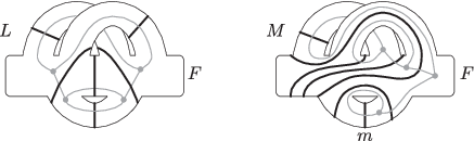
Remark 2.6.
Turning an arc corresponds to applying an IH-move of a trivalent spine.

It can be seen that Theorem 2.1 follows from Theorem 2.7 below by considering Remarks 2.3 and 2.6. We will show Theorem 2.7 instead of proving Theorem 2.1, in this section.
Theorem 2.7.
If and are markings on a surface with boundary, then there exists a finite sequence of markings on such that
- •
(resp. ) and (resp. ) are ambient isotopic in , and
- •
and are related by turning an arc for any with .
We prepare some notations that are needed for the proof of Theorem 2.7. Let and be markings on a surface with boundary such that intersects transversally, denoted by . We write
Markings and are in taut position if there is no disk such that is bounded by a 2-gon consisting of parts of and or by a 3-gon consisting of , and as illustrated in Fig. 7. Let be an arc such that . An endarc of (resp. ) is an arc contained in (resp. ) such that one point of is in and the other point is in and . We note that the number of endarcs of is equal to . For an endarc of , we denote by the arc in satisfying that has an intersection with .

Lemma 2.8.
Let and be markings on a surface with boundary such that and are in taut position. For any endarc of , the arc is turnable.
Proof.
Suppose that is not turnable. The configuration of is as illustrated in Fig. 8, where we remember that is the connected component of that contains . One point of is in , and the other point of is in the boundary of an annulus or a Möbius band as illustrated in Fig. 8. In each of the cases, a contradiction occurs for our assumption that and are in taut position. Therefore, is turnable. ∎

Lemma 2.9.
Let and be markings on a surface with boundary satisfying that . Then, and are ambient isotopic in .
Proof.
We deform by an isotopy of so that , that is, . We take a regular neighborhood of in . By an isotopy of , we move so that : such an isotopy exists, since is a marking. We show that each connected component of , which is a disk, contains exactly one arc of as a subset and the arc is parallel to an arc of .
Let be an arc, and let be the connected component of that contains . Since is a marking, and any arc bound no disks in . Then, is parallel to . If contains two and more arcs of , the arcs are parallel each other. This leads to a contradiction, since is a marking. Then, each connected component of contains no arcs of or contains exactly one arc of . By Lemma 2.4, if a connected component of contains no arcs, this leads to a contradiction with . Hence, every connected component of contains exactly one arc, and and are parallel. Therefore, and are ambient isotopic in . ∎
Lemma 2.10.
Let and be markings on a surface with boundary such that and are in taut position and . Then, there is a marking such that and are related by finitely many turnings of arcs and .
Proof.
In this proof, for any marking on , we write and for short notations. Let be an arc in such that .
Case 1: we suppose that . Let be an endarc of , and we put . Since and are in taut position, is turnable by Lemma 2.8, that is, is an open disk. We take a proper arc located along as illustrated in Fig. 9: is close enough to and , where it may hold that , although are not illustrated. By turning into in , we obtain a new marking on . Now, and are in taut position. Then, any endarc of that has no intersections with is also an endarc of . Any endarc of satisfying that and is contained in an endarc of . Both and the other endarc of disappear from . Since the number of endarcs of is equal to for any marking , we have ; then . Since , we have .

Case 2: we suppose that . Set . Let be an endarc of , and we put . Since and are in taut position, is turnable, that is is an open disk. Let be the arc contained in such that , and . Let the arc in such that and , see the left in Fig. 10.
We take a proper arc located partially along and as illustrated in the right of Fig. 10: is close enough to a part of and , and there is a possibility that has intersections with , although is not illustrated in Fig. 10. By turning into in , we have a new marking . Note that is an endarc of , and is also an arc in .

We show that (i) and (ii) . Now, and are in taut position. Then, by the configuration of , any endarc of is also an endarc of , contains an endarc of , or is contained in an endarc of . Since the number of endarcs of is equal to for any marking , we have , then (i) holds. The arc has an intersection with and has no intersections with ; then we have , that is, (ii) holds.
If the inequality holds, the proof completes. Then, we suppose that . Since and are also in taut position by the configuration of , the arc is also turnable by Lemma 2.8, that is, is an open disk; the shaded region in Fig. 10 is a half part of . If , the proof completes by considering Case 1. Then, we suppose that .
In the same way to construct , we continue turning arcs along a part of while keeping fixed; that is, we recursively define , , and a marking for each integer until it holds that or for some integer . Note that is the endarc of such that , and , see Fig. 11. By the above process, we obtain a sequence of markings satisfying that
for any with , in the same manner as (i) and (ii).
It suffices to show that is finite; then we suppose that is infinite. We prepare notations only for this proof. For arcs and with , we write if as a subset of or there is an integer with such that and as a subset of . For arcs and , is a descendant of if there is a finite sequence , …, of proper arcs in such that , and for any with . An arc is infinite-type if continues to be turned endlessly, that is, for any integer , there exists an integer with such that , where is the descendant of . We put
for any integer , where we define as a multiset, that is, each element of has the multiplicity. Let be an integer large enough such that all descendants of are no longer turned in for any with . By the inequality (ii′), after several times turnings, an arc with disappears, and a new arc with appears instead. Therefore, there exists an integer such that or that the multiplicity of is less than that of , where we remember that is a multiset. Hence, is 0 for an integer large enough with . This leads to a contradiction with the infiniteness of ; then is finite. ∎

Proof of Theorem 2.7.
Let and be markings on a surface with boundary. If , the proof completes by Lemma 2.9; then we assume that . By an isotopy of , we deform so that and are in taut position and . By Lemma 2.10, by finitely many turnings of , we have a marking such that . By continuing the same operation, we have a finite sequence , , …, of markings such that . Therefore, and are ambient isotopic in by Lemma 2.9. ∎
3. A diagram of a spatial surface with boundary
We regard as the one-point compactification of the Euclidean space . We regard as the set and regard as . Note that . Let be the canonical projection.
A spatial surface is a compact surface embedded in . A spatial closed surface is a spatial surface that is a closed surface. A spatial surface with boundary is a spatial surface that is a surface with boundary. A spatial surface that has connected components is said to be of -components. In Sections 3 and 4, we call a spatial surface with boundary a spatial surface for short, unless we note otherwise. If a spatial surface has intersection with , we can deform the spatial surface so that it is contained in by perturbation around ; then we assume that a spatial surface is contained in . A disk embedded in is unique up to ambient isotopy; then we assume that a spatial surface has no disk components throughout this paper.
For the same reason as the case of spatial surfaces, we assume that a spatial graph is contained in . A spatial graph is in semiregular position with respect to if it satisfies that
- •
has finitely many multiple points, that is,
is finite, - •
any multiple point is a double point or a triple point, that is,
- •
for any distinct trivalent vertices and of ,
- •
contains no vertices of for any triple point ,
- •
there are three disjoint arcs , and in such that , and intersect transversally at for any triple point .
Let be a spatial graph in semiregular position. A multiple point is regular if , contains no vertices of and there are two disjoint arcs and in such that and intersect transversally at . A multiple point is non-regular if is not regular. We note that any multiple point is non-regular if has vertices. A spatial graph is in regular position with respect to if it satisfies that
- •
is in semiregular position with respect to , and
- •
every double point is regular.
A projection of spatial graphs is the image of a spatial graph in regular position. A spatial graph diagram is a pair of a projection of spatial graphs and under/over information at every double point. For a spatial graph in regular position, we denote by the spatial graph diagram satisfying that the projection of is and that the under/over information at each double point is directly obtained from .
We denote by the set of -valent vertices of a graph . In this paper, we regard a spatial graph diagram as a graph; we denote by the set of -valent vertices of . A -graph is a graph whose any vertex is bivalent or trivalent. Note that a trivalent graph is a kind of 2,3-graph.
Definition 3.1.
For a spatial -graph diagram , we call a map a sign of . A spatial surface diagram is a pair of a spatial 2,3-graph diagram and a sign of .
Although any spatial trivalent graph diagram has no bivalent vertices, we regard the empty function as a sign of . For a spatial surface diagram , we construct an unoriented spatial surface by operations as illustrated in Fig. 12: an arc is replaced with a band, a bivalent vertex is replaced with a twisted band, and one of two crossed bands is slightly perturbed into the direction of the z-axis around each crossing. An example of a spatial surface diagram and its spatial surface is illustrated in Fig. 13.

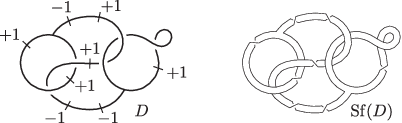
Definition 3.2.
The Reidemeister moves for a spatial surface diagram are defined as illustrated in Fig. 14: each area outside of a dotted circle is not changed before and after the replacement.
Spatial surface diagrams and are said to be related by R0–R6 moves in (resp. ) if there exists a finite sequence of spatial surface diagrams with and such that is transformed into by one of R0–R6 moves in (resp. ) for any .
Remark 3.3.
An R move is realized by using R0 and R1 moves.
As is mentioned in Lemma 4.1 (1), for an arbitrary unoriented spatial surface , there is a spatial surface diagram such that and are ambient isotopic in , where we call a diagram of , hereafter. Theorems 3.4 and 3.5 below are main theorems in this paper.
Theorem 3.4.
Let and be diagrams of unoriented spatial surfaces and , respectively. Then, the following conditions are equivalent:
- (a)
and are ambient isotopic in .
- (b)
and are related by R0–R6 moves in .

Next, we consider oriented spatial surfaces. Let be a spatial surface diagram with no bivalent vertices; is orientable. We give an orientation for as illustrated in Fig. 15: a side of facing the positive direction of the z-axis is defined as a front side and the other side of is defined as a back side. We denote by the spatial surface equipped with the above-mentioned orientation.

As is mentioned in Lemma 4.1 (2), for any oriented spatial surface , there is a spatial surface diagram with no bivalent vertices such that and are ambient isotopic in including orientations, where we call a diagram of , hereafter.
Theorem 3.5.
Let and be diagrams of oriented spatial surfaces and , respectively. Then, the following conditions are equivalent.
- (a)
and are ambient isotopic in including orientations.
- (b)
and are related by R, R2–R3 and R5–R6 moves in .
- (c)
and are related by R2–R3 and R5–R6 moves in .
The proofs of Theorems 3.4 and 3.5 are written in Section 4. When we deal with a spatial surface that contains closed components, we consider a spatial surface with boundary that is obtained by removing an open disk in each closed component. Details are described in Section 5.
Remark 3.6.
In [4], Ishii established Reidemeister moves of handlebody-links. The Reidemeister moves of handlebody-link is the R1–R6 moves in Fig. 14 by omitting all signs. We obtain the Reidemeister moves of oriented spatial surfaces by removing R1 and R4 moves of that of handlebody-links. Then, we also call an oriented spatial surface a framed handlebody-link.
4. The proofs of Theorems 3.4 and 3.5
Throughout Section 4, a bivalent vertex of a spatial surface diagram is denoted by a black (resp. white) vertex if (resp. ), see Fig. 16. A spatial surface is already defined in Definition 3.1. However, in Section 4, we replace each bivalent vertex with the band as illustrated in Fig. 16 to avoid complication of figures: twisted bands in Fig. 16 and Fig. 12 are ambient isotopic in a local area.

We prepare some notations used in proofs. Let and be a spatial surface diagram and a trivalent spine of , respectively. A proper arc in is a corner-arc if the restriction is not injective for any neighborhood of any point , see Fig. 17. We denote by the disjoint union of corner-arcs of . The pair is in semiregular position if
- •
, which is a spatial graph, is in semiregular position (see Section 3), and
- •
is finite, that is, has intersection with at finitely many points.

When is in semiregular position, has no triple points, since and for any . Suppose that is in semiregular position. A point is transversal if is not a trivalent vertex of and and intersect transversally at . A point is non-transversal if is not transversal. A trivalent vertex is non-transversal if it is in . The pair is in regular position if
- •
is in semiregular position,
- •
is in regular position (see Section 3), and
- •
any point in is transversal.
Suppose that is in regular position. We explain a way to construct a spatial surface diagram . First, we replace every point in with a bivalent vertex. We regard as the spatial 2,3-graph obtained by adding bivalent vertices. Next, we define a sign of . We fix a “thin” regular neighborhood of in ; and are ambient isotopic in . For every bivalent vertex in , which is on a corner-arc of , we define by observing a peripheral area around as depicted in Fig. 18. Then, we have the spatial surface diagram , denoted by hereafter.

We also write . We often assume that is in , that is, we identify with .
The lemma below claims that any spatial surface can be presented by spatial surface diagrams.
Lemma 4.1.
Let be an spatial surface.
- (1)
There is a spatial surface diagram such that and are ambient isotopic in .
- (2)
If is orientable and oriented, then there is a spatial surface diagram with no bivalent vertices such that and are ambient isotopic in including orientations.
Proof.
We describe an example of ways to construct a diagram of .
We prove (1). By perturbing slightly, we deform so that and is injective for some open subset of and each connected component of . We fix an arbitrary trivalent spine of . By an isotopy of , we deform so that every trivalent vertex of is contained in . We perturb the z-axis of the canonical projection slightly so that is in regular position. Next, we take a thin enough neighborhood of in . If necessary, we deform any twisted part of into the configuration in Fig. 16 so that is in regular position. Since , and are ambient isotopic, is a diagram of .
We prove (2). By the consequence of (1), there is a spatial surface diagram such that and are ambient isotopic, where we forget the orientation of . We regard as . Let be a 2,3-spine of such that . By an isotopy of , we deform the oriented surface so that any front side of peripheral regions around trivalent vertices of faces the positive direction of the z-axis. By an isotopy of that keeps any peripheral region of trivalent vertices fixed, we deform so that is in regular position and has no corner-arcs: all full twisted bands are deformed as illustrated in Fig. 19. Then, we obtain a spatial surface diagram with no bivalent vertices such that and are ambient isotopic in including orientations. ∎

4.1. The proof of Theorem 3.4
For also spatial trivalent graph diagrams, Reidemeister moves are defined as illustrated in Fig. 20 (cf. [6]). Two spatial trivalent graph diagrams are related by Reidemeister moves if and only if the two spatial graphs are ambient isotopic in . We use the same symbols as the spatial surface diagrams; an R2, R3 or R5 move of Fig. 20 is the same as that of Fig. 14.
For a spatial surface diagram , let us denote by the spatial trivalent graph diagram that is obtained from by forgetting its bivalent vertices. A spatial surface is well-formed if for some spatial surface diagram , where this notation is used only in Lemma 4.2.

Let be an isotopy with , and let be a spatial graph. For , the image has a critical point if there is a small open interval with such that
- •
is in regular position with respect to for any , and
- •
a transversal crossing of projections of occurs or disappears around before and after as illustrated in Fig. 21.

Lemma 4.2.
Let be a spatial surface diagram, and we put . We denote by the trivalent spine of satisfying . Let be an isotopy with such that is well-formed and is in regular position. Then, and are related by R0–R5 moves in .
Proof.
For any subset in and any , we write . We slightly perturb the isotopy or the z-axis of the canonical projection so that the following conditions are satisfied:
- •
is in semiregular position for any ,
- •
is finite,
- •
is finite and ,
- •
if , then has exactly one non-regular multiple point,
- •
if , then has exactly one critical point.
We note that is in regular position for any . For any , we write , which is a spatial trivalent graph diagram. Note that and . Let , , …, be all points in such that , where we put . We put for any integer with , where we set and .
By adding bivalent vertices and signs to the sequence of spatial trivalent graph diagrams, we will construct a sequence of spatial surface diagrams with such that and are related by R0–R5 moves for any with and any and . Furthermore, we will show that and are related by R0 moves; then the proof will complete.
First, we recursively construct a sequence of spatial surface diagrams satisfying for any . We set . We define for any as follows: and are related by an isotopy of and . Suppose that is already defined. We define by the following procedures.
Case 1: we consider the case that , that is, an R1 (resp. R4) move of Fig. 20 is applied before and after in . Let be a small region in which the move is applied. If a bivalent vertex of the corresponding spatial surface diagram is contained in , we move the vertex on the outside of by using R0 moves. By adding bivalent vertices, we define for any as illustrated in Fig. 22: R0 and R1 (resp. R4) moves of Fig. 14 are applied before and after , , and and are related by R0 moves and an isotopy of for any . The case of applying the right R1 (resp. R4) move of Fig. 20 is omitted.

Case 2: we consider the case that , that is, a move except for both R1 and R4 moves of Fig. 20 is applied before and after in . If a bivalent vertex of the corresponding spatial surface diagram is contained in , we move it on the outside of by R0 moves. By adding no bivalent vertices, we define for any as follows: is equal to in , , and and are related by R0 moves and an isotopy of for any . Before and after , a move that is not illustrated in Fig. 20 may be applied, however, and are actually related by R2, R3 and R5 moves; two examples of a move that is not illustrated in Fig. 20 are depicted in Fig. 23.

By the processes, we have of spatial surface diagrams satisfying that for any ; then and are related by R0–R5 moves.
Secondly, we show that and are related by R0 moves, where we note that . We take a thin enough regular neighborhood of in so that is a regular neighborhood of in for any . Now, is a disjoint union of handlebodies embedded in , and is a spatial surface properly embedded in , that is, and .
Although each is properly embedded in , we regard that each is also properly embedded in and that contains for any , where we note that is also a spine of . We regard that . By the construction of , the spatial surfaces and are related by an isotopy satisfying that , and for any and any . Let be an edge of . Since keeps fixed, then there exist bands and such that and , where each of and is a closed interval. An example of is illustrated in Fig. 24.

The sum of the sign of vertices on in is equal to that in . Therefore, and are related by R0 moves. ∎
Lemma 4.3.
Let be a spatial surface diagram, and put . Let be a trivalent spine of such that is in regular position. Then,
- (1)
and are related by R0–R2 and R4–R6 moves in , and
- (2)
and are related by R2 and R5–R6 moves in , if has no bivalent vertices.
Proof.
We show (1). Let be the spine of satisfying . Since two trivalent spines are related by finitely many IH-moves and isotopy (Theorem 2.1), it suffices to show that and are related by R0–R2 and R4–R6 moves moves if and are related by exactly one IH-move or an isotopy in .
First, we suppose that and are related by an isotopy in ; we show that and are related by R0–R2 and R4–R5 moves moves. Let be an isotopy of with such that . Write for any . We slightly perturb the isotopy or the z-axis of so that the following conditions are satisfied:
- •
is in semiregular position for any ,
- •
is finite,
- •
is finite and ,
- •
if , then
- –
has exactly one non-transversal intersection with and any double point of is regular, otherwise
- –
has exactly one non-regular double point and any intersection of with is transversal,
- –
- •
if , then has exactly one critical point,
Put . For any , is in regular position; is well-defined. We check the sequence of spatial surface diagrams in detail. Let be an point in .
Case 1: we consider the case where and has one non-transversal intersection with . We note that any double point of is regular. Suppose that is not a trivalent vertex. Before and after in , one of the deformations in Fig. 25 is applied, although the case where an arc passes through a corner-arc from the back side of is omitted. Each deformation is realized by R0–R1 moves. We suppose that is a trivalent vertex. Before and after in , one of the deformations in Fig. 26 is applied, although the case where a vertex passes through a corner-arc from the back side of is omitted. Each deformation is realized by R0 and R4 moves.
Case 2: we consider the case where and has one non-regular double point. We note that any intersection of with is transversal. Since no arcs pass through a corner-arc before and after , then R0 moves are not applied in before and after . A deformation before and after in are realized by R2 and R5 moves.


Case 3: we consider the case where . We note that is in regular position. There is a transversal point such that is the critical point. One of the deformations in Fig. 27 is applied in before and after . Each deformation is realized by R0–R1 moves.
By considering the cases above, and are related by R0–R2 and R4–R5 moves, where we note and .
Secondly, we suppose that and are related by an IH-move on ; we show that and are related by R0–R2 and R4–R6 moves. When an IH-move is applied, there might be many arcs above or below the region where the IH-move is applied. Then, we shrink the region, by isotopy of , into a small region so that an R6 move can be applied. In the process of shrinking the region, R0–R2 and R4–R5 moves are applied, see the cases 1, 2 and 3. Hence, and are related by R0–R2 and R4–R6 moves.

We show (2). Since has no corner-arcs, none of R0–R1 and R4 moves are not applied, see the case 1, 2 and 3. Therefore, and are related by R2 and R5–R6 moves. ∎
Proof of Theorem 3.4.
Since and are ambient isotopic, we assume that . For the same reason, we assume that .
Suppose that (b) is satisfied. If and are related by exactly one of R0–R6 moves, we can immediately construct an isotopy between and . Since and are related by finitely many R0–R6 moves, then and are also ambient isotopic; (a) holds.
Suppose that (a) is satisfied; we show that (b) holds. Let (resp. ) be the trivalent spine of (resp. ) such that (resp. ). Since and are ambient isotopic, we take an isotopy with such that and is in regular position. By Lemma 4.2, and are related by R0–R5 moves. Furthermore, and are related by R0–R2 and R4–R6 moves by Lemma 4.3 (1). Therefore, and are related by R0–R6 moves. ∎
4.2. The proof of Theorem 3.5.
Lemma 4.4.
Proof.


For a spatial surface diagram , let us denote by the spatial surface diagram that is obtained from by forgetting its bivalent vertices: has no bivalent vertices, and the sign of is the empty function. An edge of the spatial surface diagram is a part of such that corresponds with the projection image of an edge or a loop component of the trivalent graph which represents. A self-crossing of is positive (resp. negative) if it is the left (resp. right) self-crossing of Fig. 31: a dashed line may have crossings with other arcs of .

Definition 4.5.
For an edge of a spatial surface diagram , let us denote by and the number of positive and negative self-crossings of , respectively. We define the framing of as , where we write .
Lemma 4.6.
If we apply R0–R3 moves for a spatial surface diagram, the framing of each edge does not change.
Proof.
We can check easily that the framing of each edge does not change before and after an R0, R1, R2 or R3 move. ∎
Remark 4.7.
Applying an R4 move to a spatial surface diagram changes the framing of an edge. There is a possibility that an R5 move changes the framing of an edge.
We denote by R1 the Reidemeister move R1 that reduces the number of crossings.
Lemma 4.8.
Let be a sequence of spatial surface diagrams such that
- •
and have no bivalent vertices and
- •
is transformed into by an R0 move or an R1 move for any .
Then, and are related by R and R2–R3 moves in .
Proof.
By our assumption, we see that is obtained by continuing to replace an local arc of with a teardrop-like piece, see Fig. 32. On each edge of , we move teardrop-like pieces into a small region so that all the teardrop-like pieces of an edge are aligned as depicted in Fig. 33. When a teardrop-like piece is passing through a crossing, R2–R3 moves are applied, see Fig. 34. By the process, we have a new spatial surface diagram such that and are related by R2–R3 moves.
We show that and are related by R and R2–R3 moves; then the proof will be shown. Since and are related by R0–R1 moves, and are related by R0–R3 moves. By Lemma 4.6, the framing of each edge does not change before and after the process above. Therefore, in each local area where the teardrop-like pieces are gathered, the number of positive self-crossings is equal to that of negative self-crossings. In Fig. 33, the B and C parts are canceled by R2–R3 moves by Lemma 4.4 (1), and the A and D parts are also canceled by R moves by Lemma 4.4 (2). Hence, and are related by R and R2–R3 moves. ∎



The lemma below follows immediately.
Lemma 4.9.
Let and be spatial surface diagrams. We suppose that has no bivalent vertices. If and are related by R0, R2–R3 and R5 moves in , then and are related by R2–R3 and R5 moves in , and and are related by R0 moves.
Proposition 4.10.
Let and be spatial surface diagrams that have no bivalent vertices. If and are related by R0–R3 and R5 moves in , then and are related by R, R2–R3, and R5 moves in .
Proof.
It suffices to construct a spatial surface diagram with no bivalent vertices such that and are related by R2–R3 and R5 moves and that and are related by R, R2–R3, and R5 moves.
Since and are related by R0–R3 and R5 moves, we fix a sequence of spatial surface diagrams related by R0–R3 and R5 moves such that and . Modifying the sequence , we will recursively construct a new sequence of spatial surface diagrams satisfying that and are related by R0, R2–R3 and R5 moves for every with . We set . Suppose that is already defined.
Case 1: we consider the case where and are related by an R1 move. We suppose that the left R1 move in Fig. 14 is applied. As is illustrated in Fig. 35, we define for two cases: we attach a “small bivalent disk” on spatial surface diagrams, in stead of applying the left R1 move in Fig. 14. Each small bivalent disk contains one teardrop-like part and two bivalent vertices. At a glance, and seem to be related by an R1 move. However, and are actually related by R0 and R2 moves. If a small bivalent disk attached to is contained in the region where an R1 move is applied, we move it into on the outside of the region by using R0 and R2–R3 moves before we define , see Fig. 36. For also the right R1 move in Fig. 14, we define in the same manner.
Case 2: we consider the case where and are related by one of R0, R2–R3 and R5 moves. Let be a disk in which the moves is applied. If a small bivalent disk attached to is contained in , we move it on the outside of by using R0 and R2–R3 moves before we define , as is the case 1. We define as follows: is equal to in the outside of and the part of contained in corresponds to the applied move.


By the above definitions, we obtain a sequence such that and are related by R0, R2–R3 and R5 moves for any . Then, and are related by R0, R2–R3 and R5 moves. Hence, by Lemma 4.9, (i) the spatial surface diagrams and are related by R2–R3 and R5 moves, and and are related by R0 moves. On the other hand, is transformed into by using R0 and R1 moves in each small bivalent disk. Then, is also transformed into by using R0 and R1 moves. By Lemma 4.8, we understand that (ii) and are related by R, R2–R3 and R5 moves in . By using (i) and (ii), and are related by R, R2–R3 and R5 moves. ∎
We denote by R4 (resp. R4) the Reidemeister move R4 that reduces (resp. increases) the number of crossings.
Lemma 4.11.
Let be a sequence of spatial surface diagrams satisfying that
- •
is transformed into by an R4 move for any , and
- •
R4 moves are applied an even number of times at each trivalent vertex in .
Then, and are related by R0–R3 and R5 moves in .
Proof.
It is sufficient to prove that and are related by R0–R3 and R5 moves if R4 moves are applied exactly two times at each vertex in . All situations around a trivalent vertex of are depicted in Fig. 37: each local part in the figure is transformed into a Y-shaped part by using two R4 moves.


Proposition 4.12.
Let be a sequence of spatial surface diagrams satisfying that
- •
both and have no bivalent vertices,
- •
and are related by one of R0–R5 moves for any , and
- •
R4 moves are applied an even number of times at each trivalent vertex in .
Then, and are related by RR2–R3 and R5 moves in .
Proof.
We will show that and are related by R0–R3 and R5 moves; then and are related by R, R2–R3 and R5 moves by Proposition 4.10, that is, the proof will complete. It suffices to construct a sequence of spatial surface diagrams with and satisfying that
- (i)
and are related by R0–R3 and R5 moves for any integer ,
- (ii)
is transformed into by an R4 move for any integer with ,
- (iii)
R4 moves are applied an even number of times at each trivalent vertex in ,
since and are related by R0–R3 and R5 moves by Lemma 4.11.
First, by modifying the given sequence , we recursively construct a sequence of spatial surface diagrams. We set . Suppose that is already defined.
Case 1: we consider the case where and are related by an R4 move. Suppose that the left R4 move in Fig. 14 is applied. Let be the trivalent vertex in which the move is applied. We define as illustrated in Fig. 39: we replace in with a “small trivalent disk”, instead of applying the left R4 move in Fig. 39. Each small trivalent disk contains an trivalent vertex and three bivalent vertices. At a glance, and seem to be related by an R4 move. However, and are actually related by R0 and R2 moves. If a trivalent vertex is already replaced with a small trivalent disk, we think of the trivalent disk as a trivalent vertex. In the case, the small trivalent disk contains a smaller trivalent disk. For the case where the right R4 move in Fig. 14 is applied, we define in the same manner.

Case2: we consider the case where and are related by an R0–R3 or R5 move. Suppose that an R0, R1, R2 or R3 move is applied in a region . We define the spatial surface diagram as follows: is equal to on the outside of , and is equal to on the inside of . Suppose that an R5 move is applied in a region . If contains no trivalent small disk, we define in the same way above. If contains trivalent small disks, we regard the outermost small trivalent disk as a trivalent vertex and define in the same way above. In this case, and are related by R0, R2–R3 and R5 moves, see Fig. 40.

By the construction above, (i) holds.
Secondly, we construct a sequence of spatial surface diagrams. We continue applying R4 moves in order starting from the innermost small trivalent disks of , until trivalent disks disappear. We have , finally. Let be a sequence obtained by the above process satisfying that and the condition (ii). The number of R4 moves in is equal to the number of R4 moves in at each trivalent vertex. Since R4 moves are applied an even number of times at each trivalent vertex in , then the condition (iii) holds. ∎
Proof of Theorem 3.5.
Since and are ambient isotopic, we assume that . For the same reason, we assume that .
We suppose that (b) holds; we show that (c) holds. By Lemma 4.4 (2), an R move is realized by R2–R3 and R5 moves in ; then (c) holds.
We suppose that (c) holds; we show that (a) holds. If and are related by exactly one of R2–R3 and R5–R6 moves, we can immediately construct an isotopy between and that preserves the orientations of and . Since and are related by finitely many R2–R3 and R5–R6 moves, then and are also ambient isotopic including orientations: (a) holds.
We suppose that (a) holds; we show that (b) holds. Let (resp. ) be the trivalent spine of (resp. ) such that (resp. ). Since and are ambient isotopic including orientations, we fix an isotopy with such that including orientations, and that is in regular position. By Lemma 4.3 (2), and are related by R2–R3 and R5–R6 moves in . Then, it suffices to show that and are related by R, R2–R3 and R5 moves in . By Lemma 4.2, and are related by R0–R5 moves. Let be a sequence of spatial surface diagrams with and such that and are related by one of R0–R5 moves for any , where we note that both and have no bivalent vertices. Since the orientation of the oriented spatial surface is equal to that of the oriented spatial surface , then R4 moves are applied an even number of times at each trivalent vertex in . Hence, satisfies all of the conditions in Proposition 4.12. By Proposition 4.12, and are related by R, R2–R3 and R5 moves. ∎
5. A diagram of a non-split spatial surface
In Sections 3 and 4, we called a spatial surface with boundary a spatial surface for short. In this section, we use the notion of a spatial surface in the original definition: a spatial surface may have some closed components, see Section 3. We assume that a spatial surface has no sphere components and no disk components, since a sphere or disk in is unique up to ambient isotopy.
A spatial surface is split if there is a 2-sphere embedded in such that bounds no balls in . A spatial surface is non-split if is not split, that is, any sphere embedded in bounds a ball. We note that any 1-component spatial surface is always non-split.
In this section, we consider a way to present non-split spatial surfaces. Let be a non-split spatial surface. If has closed components , …, , we remove the interior of a disk from . By the finitely many operations of removing a disk interior in each closed component, we have a spatial surface with boundary, where we put . Proposition 5.1 claims that has necessary and sufficient information of the original spatial surface up to ambient isotopy. Therefore, when we deal with a spatial surface that has closed components, it is sufficient to consider a spatial surface with boundary that is obtained from the original spatial surface by removing a disk interior of each closed component.
Proposition 5.1.
Let be a non-split spatial surface, and let be a disjoint union of disks in . We denote by the non-split spatial surface . Let be a disjoint union of disks in such that for any integer with . Then, the spatial surfaces and are ambient isotopic in .
Proof.
We use the Cut-And-Paste method. By an isotopy of , we deform so that is minimal, where we put , and is the number of connected components of .
We show that ; we suppose that . We may assume that every connected component of is a loop. We take an innermost disk on , where we note and is a loop in . Put . Let be the disk on such that . Let be a thin regular neighborhood of in , where we note that is an annulus in . Let (resp. ) be the loop of such that (resp. ). Let (resp. ) be a disk in such that (resp. ) is parallel to and (resp. ). Put . Since is non-split, the sphere bounds a ball in . Then, and are ambient isotopic in . On the other hand, is less than , where we put . This leads to a contradiction with the minimality of . Hence, .
We put for any integer with , where we note that is a disjoint union of spheres embedded in . Since is non-split, each sphere bounds a ball in ; then . Let and be integers with . If , it holds that , and we have , since . This leads to a contradiction. Hence, we have , that is, ; therefore the balls , …, are pairwise disjoint.
In each ball , we deform into by an isotopy of . Therefore, the spatial surfaces and are ambient isotopic in , where we note that . ∎
In Proposition 5.1, if is split, the claim does not always hold because there is no information about a “partition” of by the closed components of .
Theorem 5.2.
Let (resp. ) be a non-split unoriented spatial surface. Let (resp. ) be the non-split unoriented spatial surface with boundary that is obtained from (resp. ) by removing an open disk from every closed component. Let (resp. ) be a diagram of (resp. ). Then, the following conditions are equivalent.
- (a)
and are ambient isotopic in .
- (b)
and are related by R0–R6 moves in .
Proof.
Suppose that (a) is satisfied. We show that (b) holds. Let (resp. ) be a disjoint union of disks contained in (resp. ) such that (resp. ). Since and are ambient isotopic in , we take an isotopy such that and . Then, and are ambient isotopic in . On the other hand, since and are ambient isotopic in , the spatial surfaces and are ambient isotopic in ; then and are also ambient isotopic in . Therefore, and are ambient isotopic in . By Theorem 3.4, and are related by R0–R6 moves in .
Theorem 5.3.
Let (resp. ) be a non-split oriented spatial surface. Let (resp. ) be the non-split oriented spatial surface with boundary that is obtained from (resp. ) by removing an open disk from every closed component. Let (resp. ) be a diagram of (resp. ). Then, the following conditions are equivalent.
- (a)
and are ambient isotopic in including orientations.
- (b)
and are related by R, R2–R3 and R5–R6 moves in .
- (c)
and are related by R2–R3 and R5–R6 moves in .
Next, we explain relations among knots, handlebody-knots and spatial surfaces. For a manifold embedded in , we denote by the ambient isotopy class of in . We put
where we note that a knot is a kind of non-split link, and a handlebody-knot is kind of non-split handlebody-link. The following maps are injective:
where means a regular neighborhood of in , and means a spatial surface with boundary obtained from by removing the interior of a disk in each closed component of . Injectivity of follows from Proposition 5.1.
By injectivity of the above maps, we have new presentation of non-split links and non-split handlebody-links by using spatial surface diagrams, see Fig. 41. This suggests a new approach to studying a knot, link, handlebody-knot and handlebody-link in a framework of spatial surfaces.

Remark 5.4.

For any component of a diagram of a link, which has no trivalent vertices, we attach an ear-like edge as illustrated in Fig. 43. The diagram, which has trivalent vertices, is denoted by .
By using Proposition 5.1, we have the following Theorem.
Theorem 5.5.
Let and be diagrams of non-split unoriented links and , respectively. Then, the following conditions are equivalent.
- (a)
and are ambient isotopic in .
- (b)
and are related by R2–R3 and R5–R6 moves.

Acknowledgements
The author would like to thank the referee, Atsushi ISHII, Koki TANIYAMA and Tomo MURAO for valuable discussions and suggestions.
References
- [1] N. Apostolakis, R. Piergallini and D. Zuddas, Lefschetz fibrations over the disk, Proc. London Math. Soc. 107 (2013), 240–290.
- [2] I. Bobtcheva and R. Piergallini, On 4-dimensional 2-handlebodies and 3-manifolds, J. Knot Theory Ramifications 21 (2012), no. 12, 1250110.
- [3] T. Homma, On the existence of unknotted polygons on 2-manifolds in , Osaka J. Math. 6 (1954), 129–134.
- [4] A. Ishii, Moves and invariants for knotted handlebodies, Algebr. Geom. Topol. 8 (2008), 1403–1418.
- [5] A. Ishii, S. Matsuzaki and T. Murao, A multiple group rack and oriented spatial surfaces, J. Knot Theory Ramifications (7)29 (2020), 2050046, 20pp.
- [6] L. H. Kauffman, Invariants of graphs in three-space, Trans. Am. Math. Soc. 311 (1989), no. 2, 2788–2794.
- [7] F. Luo, On heegaard diagrams, Math. Res. Lett. 4 (1997), 365–373.
- [8] K. Reidemeister, Knotten und Gruppen, Abh. Math. Sem. Univ. Hamburg 5 (1927), 7–23.
- [9] D. Roseman, Reidemeister-type moves for surfaces in four-dimensional space, In: “Knot theory”, Banach Center Publ. 42, Polish Acad. Sci. Inst. Math. Warsaw, 1998, 347–380.
- [10] S. Suzuki, On complexity of a surface in 3-sphere, Osaka J. Math. 11 (1974), 113–127.
- [11] Y. Tsukui, On surfaces in 3-space, Yokohama Math. J. 18 (1970), 93–104.