May 2019
Holographic conformal transition and light scalars
Alex Pomarola,b, Oriol Pujolasa and Lindber Salasa
aIFAE and BIST, Universitat Autònoma de Barcelona,
08193 Bellaterra, Barcelona
bDept. de Física, Universitat Autònoma de Barcelona,
08193 Bellaterra, Barcelona
Abstract
We present an holographic approach to strongly-coupled theories close to the conformal to non-conformal transition, trying to understand the presence of light scalars as recent lattice simulations seem to suggest. We find that the dilaton is always the lightest resonance, although not parametrically lighter than the others. We provide a simple analytic formula for the dilaton mass that allows us to understand this behavior. The pattern of the meson mass spectrum, as we get close to the conformal transition, is found to be quite similar to that in lattice simulations. We provide further predictions from holography that can be checked in the future. These five-dimensional models can also implement new solutions to the hierarchy problem, having implications for searches at the LHC and cosmology.
1 Introduction
Theories close to being conformally invariant are of utmost interest as they can generate large hierarchies of scales that can be useful in particle physics and cosmology. This motivates the understanding of how theories behave at the critical point at which, by varying the parameters of the theory, we pass from a conformal regime to a non-conformal one.
This is especially interesting in strongly-coupled theories as they can give rise to non-trivial dynamics. An example is QCD where by increasing the number of flavors , the theory is expected to become conformally invariant at some critical value . It is unclear where this exactly happens, but lattice simulations suggest that this could be around . For , QCD becomes a conformal field theory (CFT) till reaching , where is the number of colors ( for real QCD), at which the theory reaches the Banks-Zaks fixed point, becoming IR free for . The region is called the conformal window.
Recent lattice simulations suggest that, contrary to real QCD, theories close to the conformal transition have as the lightest resonance a state (apart, of course, from the Goldstone bosons, the pions) [1, 2]. It is unclear what is the origin of the lightness of this state. Some arguments suggest that this could be a dilaton, the Goldstone associated to the breaking of scale invariance. If this is the case, it would be interesting to know whether in the large- limit, where becomes a continuous parameter, the dilaton mass tends to zero as we approach the critical point from below .
In this article we would like to analyze the physics of conformal transitions using holography. We will follow Ref. [3] that argued that the exit of the conformal window of large- QCD occurs when the IR fixed point disappears by merging with a UV fixed point. Close to the conformal edge the theory contains a marginal operator whose dimension gets a small imaginary part when conformal invariance is lost (see next section for details). Assuming that this is the case, the AdS/CFT correspondence [4] can provide a simple realization of this idea as a complex operator dimension matches to a scalar having a mass below the Breitenlohner-Freedman (BF) bound . When this happens, the scalar becomes tachyonic and gets a non-zero profile that results into a departure from the Anti-de-Sitter (AdS) geometry [3].
The presence of a marginal operator in the model could suggest the presence of a light dilaton, along the lines of Refs. [5, 6]. The argument goes as follows. The dilaton potential can be written as
| (1) |
such that, when a minimum exists, leads to a dilaton mass given by
| (2) |
where and . A nonzero arises only from an explicit breaking of scale invariance. When this latter comes only from , we have , and Eq. (2) predicts . Therefore, a dilaton can be parametrically light if the dimension of is given by with (i.e., ) being a controllable small parameter till the end of the RG-flow. The holographic implementation of this is the Goldberger-Wise mechanism [7], where the operator matches to an almost massless scalar in 5D (protected by a shift symmetry) [5, 6]. Nevertheless, we will see that this is not the case at the conformal transition, as the marginal operator corresponds to a double-trace operator whose dimension is not protected along the RG-flow. Having the explicit breaking of conformal invariance arising from an almost marginal operator however will have as a consequence that the dilaton is light, although not parametrically light.
We will be working with a simple weakly-coupled AdS5 theory, with the extra-dimension cut off by an IR-brane, that will contain the basic ingredients to describe the conformal transition. We will calculate the mass spectrum of resonances and show that the lightest resonance is the dilaton (the radion of the compact extra-dimension). We will present a simple analytical formula for the mass of the dilaton that will allow to understand its lightness as a function of the change of the tachyon as we move the IR-brane. This will show that either at small or large positions of the IR-brane, the dilaton is always parametrically light. In between these two regions, we will see that the dilaton mass does not have ”room” to grow and as a consequence the dilaton is always kept light.
We will compare our results with lattice simulations, showing good agreement in the pattern of masses when the conformal critical point is approached. Furthermore, we will provide further predictions to be checked in the future by lattice simulations.
The 5D model presented here could also be useful to generate small scales and explain, for example, the difference between the electroweak scale and the Planck scale. Moreover, the presence of a light scalar can have an important impact in the searches for new resonances at the LHC as predicted in composite Higgs models.
There have been previous approaches using holography to understand the conformal transition and the existence of a light dilaton [8, 9]. We find however that these studies were not exhaustive nor conclusive. Our goal is not only to provide evidence for a relatively light dilaton, but also to explain the reasons behind this.
The article is organized as follows. In Section 2 we introduce the idea of leaving the conformal window by fixed-point merging and remark its implications. In Section 3 we present the five-dimensional model and its relation with the large and expansion. We also discuss the tachyon solution and the stabilization of the radion. Next we present the predictions for the resonance mass spectrum, presenting an analytical formula for the case when the dilaton is light, as well as discussing the other scalar and vector resonance masses. In Section 4 we compare the mass spectrum calculated within our model with that obtained from lattice simulations, and in Section 5 we discuss how these models could also be useful for explaining the smallness of the electroweak scale. Conclusions are given in Section 6. We also present two Appendices. In Appendix A we give the coupled system of equations of motion for the scalar and gravitational sectors, and derive the approximate analytical formula for the dilaton mass. In Appendix B we present the 4D effective theory of a tachyon and dilaton valid when they are the lightest states.
2 Conformal transition by fixed-point merging
There are several ways to lose an IR fixed point as we move the parameters of the theory. Either the fixed point goes to zero, to infinity or it merges with a UV fixed point. Following Ref. [3] we will consider conformal transitions characterized by the third case, the merging of the IR fixed point with a UV fixed point, as depicted in Fig. 1. In this case, the beta function can be written as
| (3) |
where is a coupling of the theory (not necessarily related to the gauge coupling in gauge theories), and depends on the parameters of the theory, e.g., . The IR and UV fixed point are respectively at
| (4) |
As we vary from negative to positive values, we have the merging of the IR and UV fixed points at , while for the theory abandons conformality, i.e., the IR fixed point is at complex coupling.
As argued in Ref. [10], for negative and close to zero, the operator with coupling must have dimension
| (5) |
and can be considered to be responsible for the RG flow towards the IR fixed point. For we have that becomes marginal, and develops a complex dimension for , signaling the end of conformality.
The above properties of this conformal transition have a straightforward holographic interpretation using the correspondence (or duality) between strongly-coupled CFT4 (in the large and large ’tHooft coupling) and weakly-coupled five-dimensional Anti-de-Sitter theories (AdS5) [4]. Operators in the CFT4 () correspond to scalars in the AdS5 () where dimensions and masses are related via the the AdS/CFT relation [4]:
| (6) |
Eq. (6) tells us that in order to have a dual of a CFT operator with complex dimension, the AdS5 must have a scalar slightly below the BF-bound, . Eq. (6) also tells us that this operator of complex dimension () has, in the limit , dimension instead of . Therefore the natural identification for the operator discussed above is , since in the large this implies and that gives us Eq. (5). In other words, must be a double-trace operator.11 1 It has been proven in Ref. [11, 10] that this is always the case for theories in the large- limit.
The existence of in the conformal transition is only an implication from large- theories, and could be not true in general. In QCD, as argued in Ref. [3], is expected to be the operator whose dimension will go from when entering the conformal window (at the Banks-Zaks fixed point) to 2 when leaving it at the other side when it becomes complex.
When the theory is close but outside the conformal window (i.e. ), one can calculate the RG flow “time” required to cross the region where and . This gives us the IR-scale at which the theory is expected to confine as becomes large. From Eq. (3) one gets
| (7) |
where is roughly the scale at which . Eq. (7) is usually referred as walking or Miransky scaling.
3 A five-dimensional model for the conformal transition
We want to study the conformal transition described above using holography. For this reason we will consider the simplest but at the same time most generic five-dimensional model containing the basic ingredients needed to describe the conformal transition via fixed-point merging. Our purpose is to generically understand the mass spectrum at the conformal transition and the presence or not of light scalars.
Let us recapitulate the basic ingredients of the theory in the 4D side. This is a strongly-coupled deformed CFT with a scalar operator, () for concreteness, whose dimension is with . This means that the scalar gets a vacuum expectation value (VEV), signaling the loss of conformality. The global symmetry of this theory is that is broken by the VEV of the scalar down to the diagonal subgroup .22 2 The U(1)A is anomalous and will not be considered here.
The corresponding holographic model will consist in a gauge theory in 5D with a complex scalar transforming as a ,. This scalar plays the role of the operator whose VEV is responsible for the breaking of the conformal and gauge symmetry, and therefore its mass will be related to the dimension of the operator. We also impose parity, defined as the interchange . The action is given by
| (8) |
where, up to dimension-four operators,33 3 Following the Effective Field Theory (EFT) approach, higher-dimensional operators are supposed to be suppressed by the cutoff scale of the model () estimated to be the scale at which the 5D theory becomes strongly coupled (i.e., when loops are as important as tree-level contributions), that is [12] – see also Section 3.1. the most general Lagrangian is given by
| (9) |
with , and being the field-strength of the , and gauge bosons respectively, and the indices run over the five dimensions, . We parametrize the fields as with Tr. The fields and will respectively transform as singlet and adjoint under the . The covariant derivative is defined as
| (10) |
and the potential is given by44 4 We notice that one can absorb one coupling into , as we will do later.
| (11) |
The 5D metric in conformal coordinates is defined as
| (12) |
where and is the warp factor. Before the scalar turns on, the presence of leads to an AdS5 geometry:
| (13) |
where is the squared AdS curvature radius.
As explained above, our important ingredient here is to consider that the conformal breaking arises when Dim[] becomes imaginary. In AdS this corresponds from Eq. (6) to take the 5D mass of below the BF bound. For this purpose, we will consider
| (14) |
When the mass of is below the BF bound and turns on in the 5D bulk, breaking the conformal and chiral symmetry . will grow as , as expected from a dimension-two perturbation in the dual 4D theory. When the energy-momentum tensor induced by the nonzero profile gets of order of the inverse 5D Newton constant, , the backreaction on the metric will be important, starting to depart then from AdS, and signaling the breaking of the conformal symmetry. This simple model, however, does not lead to a mass gap for all bulk fields, as the extra dimension is not ending at any . In fact, as we will see, the tachyon would stabilize at the minimum of the potential Eq. (11) and the metric would become again AdS. As we know that in strongly-coupled models outside the conformal window, like QCD, all resonances are heavy, we need to implement the same in our holographic version. The simplest way is to cut off the 5D space by an IR-brane at some point to be determined dynamically.
The presence of the IR-brane add extra parameters to the theory as might also have a potential on the IR-boundary. We will limit ourselves to up to quadratic terms in :
| (15) |
and study their impact on the properties of the model. We could also add to Eq. (15) quartic terms but these are not expected to change significantly our predictions, since they are suppressed by with respect to the bulk terms.55 5 Even though the same is true for the two terms in Eq. (15), these are respectively quartically and quadratically UV sensitive so they can be sizable. As it is usual in AdS/CFT, we will be regularizing the UV-divergencies by placing a UV-boundary at and taking the limit at the end of the calculation of physical quantities.
In this 5D model the two phases are determined, as in the strongly-coupled model described in Sec. 2, by the parameter:
- •
For , we have and : AdS5 (CFT4) phase.
- •
For , we have and : non-AdS5 (non-CFT4) phase.
3.1 The large and power counting
By the AdS/CFT correspondence, the 5D scalar and gauge bosons are associated to the meson operators and respectively. Therefore 5D couplings from single-trace operators must scale in this sector as . We take
| (16) |
On the other hand, double-trace operators are suppressed with respect to single-trace ones:
| (17) |
For this reason these latter terms were neglected in previous holographic approaches to QCD [13, 14]. Nevertheless, the parameter is accompanied by a factor , as we will see explicitly below (e.g. Eq. (21)), and then its effect is not suppressed for large values of . Therefore it is important to keep double-trace operators in Eq. (9) when comparing our results to strongly-coupled theories in the large and limit. In particular, will be responsible for generating a mass splitting in the scalar sector between the singlet () and the adjoint states (), as observed in lattice results with large [1, 2].
It is important to remark that we cannot consider the strict limit in our 5D model. In this limit loops of vector or scalar resonances contribute as , meaning that we cannot perform a perturbative expansion in the 5D theory. Therefore calculations will be only reliable if we take the large and large limit () keeping . Basically, the only difference here with respect to previous models for holographic QCD is the non-negligible presence of double-trace operators.
On the other hand, if we limit ourselves to the flavor-singlet sector of the theory (assuming for example that the other sectors are heavier), this can be treated perturbatively even in the strict Veneziano limit . It has been argued in Ref. [15] that there should be a dual purely closed string description of the flavor-singlet sector of the gauge theory.
From the AdS/CFT dictionary, we are also able to relate the gravitational sector of the 5D theory with the glueball sector of the 4D CFT, and derive the scaling of the 5D Newton constant with the number of colors: that using Eq. (16) implies
| (18) |
From the above we can estimate the mixing between the flavor-singlet meson sector and the glueball sector (dual respectively to the scalar and gravitational sectors in 5D) to go as
| (19) |
that becomes order one for . Therefore, contrary to previous holographic models, the impact of the gravitational sector in the singlet scalar sector cannot be neglected in this case.
3.2 The tachyon solution
The non-zero profile for will be taken to be along the direction, whose 5D Lagrangian is given by
| (20) |
where
| (21) |
being the axial-vector gauge bosons that will get masses from their coupling to . The IR-brane potential can be written as
| (22) |
Notice that the presence of a factor in front the Lagrangian means that the couplings of are suppressed by an extra with respect to those in the non-singlet sector, as expected in strongly-coupled theories in the large limit. The equation of motion (EOM) for from Eq. (20) must be solved including the metric back-reaction that via the Einstein equations (see Appendix A) determines the warp factor:
| (23) |
where from now on we will be using the dot notation: . It is important to notice that by the field redefinition we could factorize in front of the first term of Eq. (20) and make the EOM that determines the solution for independent of (only sensitive to its sign). This redefinition introduces in the interactions of with the gauge and gravitational fields (second term of Eq. (20) and Eq. (23) respectively). Nevertheless, this can be reabsorbed respectively in and , making the solutions and full mass spectrum of the model insensitive to . Therefore, with no loss of generality, we will consider .
We are interested to study the model close to the conformal transition. Therefore we will work in the limit . The solution for then only depends on , and (and the sign of ). At the UV-boundary we will impose , otherwise we would be breaking the chiral symmetry from UV-physics (as adding an explicit mass term to the quarks in the dual theory).66 6 Imposing a different boundary condition, such as , would lead to the same predictions in the limit (). On the other hand, at the IR-brane we must impose the boundary condition determined by the model:
| (24) |
where we defined . For the metric we must impose the junction condition [16]:
| (25) |
3.2.1 Region
We will start looking for solutions of the tachyon for , where we define
| (26) |
In this case non-trivial solutions from Eq. (20) fulfilling Eq. (24) are only found if the IR-brane is beyond some critical value, . It is easy to find , as this corresponds to the critical value at which we pass from having all Kaluza-Klein (KK) states of with positive squared masses to having 4D tachyons in the theory. Therefore at there must be a 4D massless mode, . The wave-function of this massless mode must satisfy the linearized bulk EOM with . We obtain [8]
| (27) |
with a normalization constant, and where the IR-boundary condition Eq. (24) at leads to
| (28) |
Notice that to have non-trivial solutions, the limit must be taken with , such that the angle in Eq. (27) is kept fixed. The presence of solutions in Eq. (28) is a well-known feature of these configurations, and it is associated to the existence of Efimov states. We will be considering , that will give us the global minimum, being the other possibilities just local minima. Eq. (28) reproduces Eq. (7) for and . The origin of the logarithm in Eq. (27), that will play an important role, can be more easily understood by looking at the strongly-coupled dual theory; this has an explicit breaking of the conformal symmetry due to the double-trace marginal operator that leads to a log-running of the couplings [17].
Depending on the position of the IR-brane with respect to , we can distinguish two limiting cases that will help to understand the physics of the model. These are illustrated in Fig. 2 and corresponds to
- I)
: In this case for all , meaning that the scale of confinement is larger than the scale of chiral breaking that is of order .
- II)
: In this case reaches values at some , and then the scale of chiral breaking is larger than the scale of confinement .
These two cases should be considered as formal limits, since in most of the parameter space of the model we will find that the IR-brane sits at few , i.e., between limits I and II, implying that naturally the scale of chiral breaking is similar to the scale of confinement.
Let us start considering the limit I, where is assumed to be just slightly above . In this case the 4D mode gets a small negative mass-squared, becoming a 4D tachyon. We find this mass is given by
| (29) |
Eq. (29) is only valid for that, obviously, requires a tuning in the parameter space: either (that we will see later cannot be achieved by the radion minimization) or that requires . To find a stable configuration this 4D tachyon must have a positive quartic self-interaction, , and this can arise either from or the feedback from gravity. We find
| (30) |
where are smooth and positive functions of as derived in Appendix B.1. The 4D tachyon VEV is then given by
| (31) |
Therefore, in the limit I the -profile of is given by Eq. (27) with Eq. (31) and , as we follow the normalization of of Appendix B.1. This solution is shown in the left plot of Fig. 2 for and . In the limit , we see from Eqs. (27)–(31) that stays constant and small. This means that the metric remains always close to AdS5.
Let us now move to the limiting case II. First, let us neglect the feedback from the metric (). As the IR-brane is now placed far away from , the tachyon profile grows till the quartic term of the potential becomes relevant. Solutions only exist if , such that settles at the minimum of the 5D potential where it takes the constant value (see right plot of Fig. 2).77 7 To satisfy the boundary condition at the IR-brane, must depart from when approaching the IR-boundary, as can be appreciated in Fig. 2. This means, in the dual interpretation, that the CFT flows at around towards another CFT in which the global symmetry has been reduced to with and respectively transforming in the singlet and adjoint representation. In this new CFT, scale invariance is broken at a much lower scale . Let us now consider the feedback of the metric. For large the gravitational feedback becomes important before reaches the minimum, making to enter into a ”slow-roll” condition (see Appendix A for details) delaying the position at which gets its maximum . In this case is also possible as the slow-roll condition keeps slowly growing till reaching the IR-brane (see right plot of Fig. 2). The metric evolves from AdS5 at to another approximately AdS5 space at .
3.2.2 Region
In this region we have that is negative, and from the left-hand side of Eq. (28), the smallest is determined by
| (32) |
that does not depend on . This means that non-trivial solutions for exist even if . These solutions however are supported by the IR-brane and for we have . Therefore as soon as the IR-brane is not stabilized for (i.e., ), we can also consider this region of the parameter space for studying the conformal transition.
In this case the solution for , as we vary , behaves in the following way. For , where is determined by , we find that takes a nonzero value with a profile localized towards the IR-brane, , as we said. The origin of this nonzero profile is that the IR-brane mass , and not the 5D mass, is exceedingly negative. is mostly constant in this region and it does not help to stabilize the IR-brane. On the other hand, for , the profile of grows to become similar to the limit II discussed before (see right-hand side of Fig. 2), indicating that behaves as a genuine 5D tachyon. This latter behavior only occurs if the 5D mass is below the BF bound and can lead to a stable IR-brane.
3.3 Radion/Dilaton stabilization
Since the position of the IR-brane is associated to a dynamical field, the radion (not necessary a mass eigenstate), its value must be determined dynamically. The extremization condition for is exactly the junction condition Eq. (25) after putting on-shell all other fields. This can be written, using Eq. (23) and Eq. (24), as
| (33) |
For our particular case, this reduces to a quadratic equation for :
| (34) |
where have introduced , , and
| (35) |
that is a measure of the detuning of the IR-brane tension away from the AdS5 value. Their values are bounded to be in the region
| (36) |
The lower bound arises from demanding that for , the IR-brane is driven to , such that the theory is in the AdS5 (CFT4) phase. From Appendix B, in particular Eq. (81), we see that is related to the self-coupling of the dilaton and comes from requiring a positive dilaton self-coupling. On the other hand, the upper limit in Eq. (36) is a more basic (geometrical) requirement: to possibly solve the junction condition even for dynamical solutions that start away from the minimum. If , the IR-brane tension is positive and it is easy to see that there would be no solutions where the IR-brane acts as an IR boundary (i.e., a cutoff of the AdS5 space at ). Therefore these regions must be discarded.

By playing with the parameters of the model, , , and , we can find regions where is stabilized thanks to the presence of the 5D tachyon. These are shown in Fig. 3 in the plane for and (left plot), and (right plot). These regions are bounded from the left and the right at which, as it will be discussed later, the radion is massless. At the left boundary one obtains the lowest value of (a stabilized) . For , this lowest value of the IR-brane position is achieved when ; for we obtain the smallest that is given by , as can be analytically found by looking at the 4D effective theory (see Appendix B). On the other hand, as we get close to the boundary on the right of the regions in Fig. 3, we have (limit II). In most of the colored regions however we have that . In other words, the model naturally predicts the scale of chiral symmetry breaking to be around the scale of confinement.
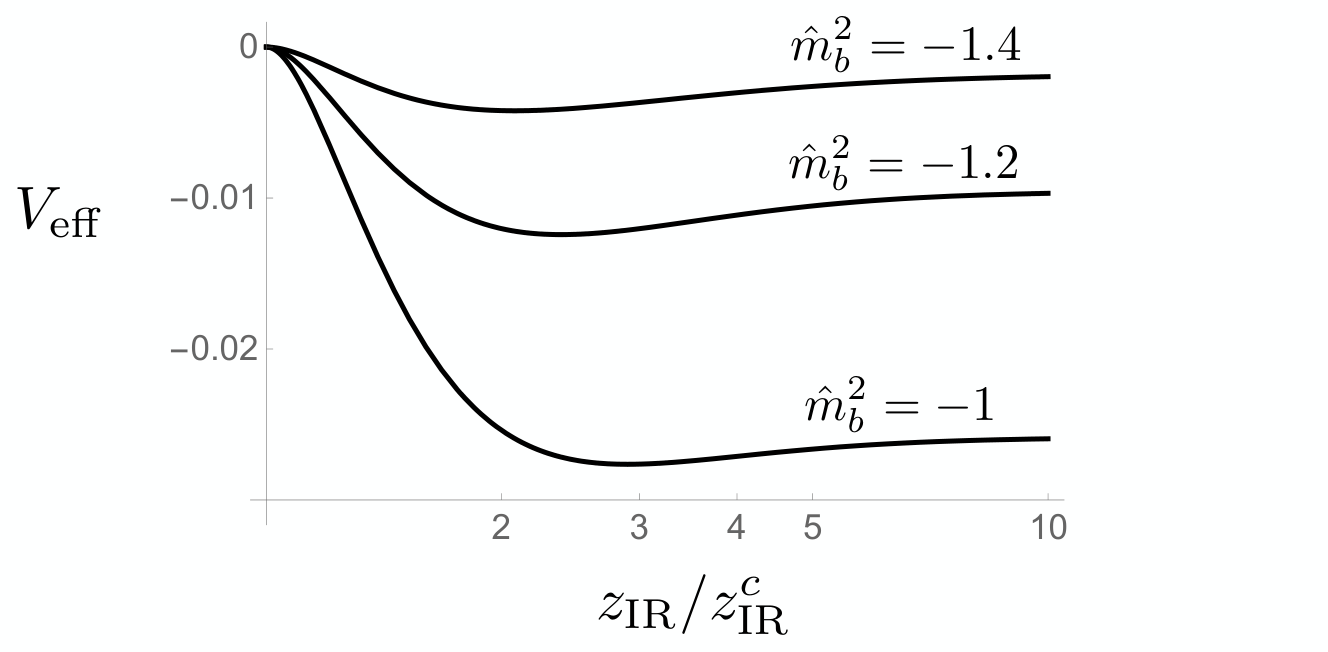
If the radion is the lightest 4D mode in the theory, we can use Eq. (33) to obtain its effective potential. The radion corresponds in the dual 4D CFT to the dilaton, , whose VEV determines the scales of the model. For this reason at the minimum is related with the warp factor evaluated at . Nevertheless, outside the minimum Eq. (33) the relation of with is a more complicated function, , especially in the basis where is canonically normalized. Going off-shell requires not equating the LHS of Eq. (33) to zero, and identifying this with the first derivative of the dilaton effective potential:
| (37) |
where is in general a complicated function of (that cannot be zero, otherwise we will have an extra minimum beyond Eq. (33)) that we do not need to specify here. By integrating Eq. (37) over , one can obtain the dilaton effective potential . For the simple case in which the backreaction is neglected and the space is just AdS5, we have and is just a constant. For this case we show the effective potential (up to an overall constant) in Fig. 4. We can see that the potential has a minimum at and goes to a constant value at large , where becomes constant as it approaches the minimum of its 5D potential. For a better understanding of the dilaton effective potential, we can analytically calculate the effective potential of the 4D tachyon and dilaton in the limit . This is done in Appendix B. This shows that the origin of the existence of a minimum in can be tracked back to the log-dependence in Eq. (29).
3.4 Excitations around the 5D tachyon
The main interest of the article is to know whether close to the conformal transition there is a light dilaton, as often claimed in the literature. Therefore we will start considering the flavor-singlet spectrum of the theory, to analyze later other sectors.
3.4.1 The singlet scalar sector and light dilaton

The flavor-singlet spectrum is composed by the radion (the only scalar in the gravitational sector) and the excitations of around the background . Since the mixing of the dilaton with is in principle sizable for (), we must consider the coupled EOM between the scalar sector and the gravitational sector. The equations for the mass spectrum are given in Appendix A.2 and must be solved numerically.
For the lightest mode the results are presented in Fig. 3 for . We have normalized the mass to the one of the lightest vector resonance, , being this latter the lightest state in real QCD and holographic versions [13, 14]. Fig. 3 shows that the state is always lighter than the vector in all regions of the parameter space. At the boundary of the regions at which IR-brane stabilization is achieved, the dilaton is massless, but its mass is roughly below half of the mass in most of the interior region. We have checked that for larger , the value of increases but not significantly.
To understand why the dilaton mass is small, it is convenient to show how its mass varies as a function of for different values of . This corresponds to moving in vertical lines in the plane of Fig. 3 from the bottom to the top, trading the parameter for by means of Eq. (34). We remark however that we will present results for a wide region of , going beyond the allowed region Eq. (36). This will help us to understand the origin of the smallness of . The result is shown in Fig. 5 for different values of . We see that the dilaton mass starts at zero at , grows for intermediate , and tends again to zero for .
We can understand this behaviour analytically. Assuming that is the radion/dilaton, we can analytically obtain its mass by taking the derivative of Eq. (37) evaluated at the minimum Eq. (33). We obtain
| (38) |
where we have used that at the minimum derived in Appendix A. In our particular case Eq. (38) reduces, after normalizing to the vector mass Eq. (46), to
| (39) |
where we have defined the dimensionless functions
| (40) | |||||
| (41) | |||||
| (42) |
with
| (43) |
where we have used Eq. (23). From Eq. (39) we can infer different regimes at which the dilaton can be light:
- •
The prefactor is suppressed for . Therefore in the limit I the dilaton is always light, even when formally we take (see discussion after Eq. (31)). Also for large values of , possible in the limit II with , we have , and consequently the dilaton mass is suppressed.
- •
The function determines the sign of . In the limit I we have and , and then becomes negative. This means that the dilaton effective potential has actually no minimum, as we already pointed out in Section 3.3. As we increase , increases till becoming zero, corresponding to the points seen in Fig. 5 with . One can check that they are inflection points of the dilaton potential.
- •
The function is the main responsible for natural light dilatons in Goldberger-Wise models [5, 6]. Since moving simultaneously the UV and IR boundaries does not change physical quantities, we can deduce
(44) showing that is in fact sensitive to the dependence of the tachyon with variations of the UV boundary, and therefore to the explicit breaking of conformal invariance (that arises due to the presence of the UV cutoff). For this reason is directly related with the beta function of the dilaton effective coupling of Eq. (1). explains why the dilaton mass always goes to zero for large . Indeed, as we approach the limit II for , the 5D tachyon goes to the minimum of its potential where it becomes constant. We then expect . Also in the limit II for the slow-roll conditions are achieved and tends to zero. Unfortunately, these regions of a parametrically light dilaton are very small in the full parameter space of the model, see Fig. 3, since stabilizing the IR-brane at large requires an adjustment of the parameters of the model. In the limit I we can derive from Eq. (27) and Eq. (31) that , and using the Eq. (82) we get that is nonzero but smallish in the regions considered.88 8 Notice that , and then does not measure the growth of the tachyon (that is power-law ), but its variation as we move the IR-brane (or UV-boundary) that it is much milder (logarithmic).
The situation is similar in regions with (see Fig. 3 or Fig. 8). The only main difference is that the dilaton mass goes to zero for small values of , not due to , but because tends to a constant value as explained in Sec. 3.2.2, and therefore .
We conclude that the dilaton mass is parametrically smaller than at small and large (respectively corresponding to the left and right boundaries of the regions of Fig. 3). At small , the reason is either the existence of an inflection point in the dilaton potential (for the case ) or that becomes frozen and (for the case ). Also at small 5D tachyon values its log-dependence on gives a smallish and therefore a smallish dilaton mass. At large (limit II) the geometry approaches again AdS5 (the dual model flows towards another approximate CFT4) where scale invariance is partially recovered and therefore the dilaton mass must go to zero. ”Trapped” between these two limits, the dilaton mass cannot grow much in the intermediate region and then remains always the lightest resonance (although not parametrically lighter than the others).
Finally, we would also like to discuss the mass of the second lightest singlet scalar, . This is also obtained numerically (see Appendix A.2), and the result is shown in Fig. 6 for certain representative values of the parameter space. This scalar is mostly the excitation around the profile (up to a small mixing with the radion), a Higgs-like state. For this reason when , we expect , as appreciated in Fig. 6.
3.4.2 Non-singlet scalars, vector and axial-vector excitations
For the scalars in the adjoint under the symmetry, , the EOM is given by
| (45) |
As we already mentioned, there are two important difference with respect the singlet scalar case. First, the scalars in the adjoint do not mix with the radion/dilaton. Second, the quartic coupling in Eq. (45) is different from the singlet case due to the presence of . This implies that the adjoint scalar masses are expected to be different from the singlet scalar masses, with the magnitude of the mass splitting being sensitive to and .
We are also interested in the vector and axial-vector spectrum [13, 14]. The vector spectrum is only indirectly sensitive to the tachyon through its impact to the metric. Therefore, since flavor-singlet resonances (the in QCD) and adjoint resonances (the in QCD) feel the same metric and have the same boundary conditions, they get equal masses. This is an important prediction of the 5D model.99 9 Of course, mass splittings could be generated at the loop level or from higher-dimensional operators in Eq. (9), but these are expected to be suppressed.
It is useful to have an approximate analytic value for , since we are using this mass to normalize the other resonance masses. This is possible in the limit in which the 5D space is approximately AdS, that corresponds to limits I and II, as we explained in Section 3.2. In AdS5 we have . We find that a reasonably good approximation for in the limit of small and large is given by Eq. (23) neglecting the derivative terms and taking at .1010 10 We put to zero the derivative terms to avoid the drastic change of near the IR boundary -see footnote 7. We then have:
| (46) |
We have checked that this value is within the exact mass of for the regions of the parameter space studied in this article.

The axial-vector spectrum depends directly on the profile via Eq. (20), being this responsible for the mass splitting from the vector spectrum. Another important quantity is the Goldstone decay constant , that is the order parameter of the chiral breaking. This can be calculated via holography from the axial-vector two-point correlator at zero momentum [13, 14]:
| (47) |
where is the 5D solution of the axial-vector with Dirichlet UV-boundary condition.
The results (with no approximations) are shown in Fig. 6 for some representative values of the parameter space. Following the notation in QCD, we denote with and the adjoint scalar and axial-vector respectively. Since is the only quantity that depends on ( in the dual theory), we have fixed its value using Eq. (51) with . For (limit I) where the chiral breaking is small, we see that indeed and are small. As we increase , we move towards limit II where the breaking of the chiral symmetry is larger, as can be appreciated by the growth of and and mass splittings. On the other hand, the mass of strongly depends on , and we have chosen a negative value, , that makes the mass splitting with the singlet sector positive, as lattice simulations (see later) seem to suggest. Similarly to the singlet scalars, we also have that goes to zero as , since the tachyon value goes to zero in this limit and we recover the chiral symmetry.
Let us briefly comment on what happens for other values of the parameters of the model. The effect of in the mass spectrum is clear from Fig. 6 where we show the spectrum for two different values of . The main effect is that as we increase , the profile of becomes flatter and smaller, as appreciated in Fig. 2, giving a smaller breaking of the chiral symmetry. The spectrum is mildly sensitive to the values of , unless we take that we will discuss later (Fig. 8). Finally, only affects and that will increase as increases.

It is more instructive, also in part to compare later our results with lattice simulations, to analyze the spectrum at constant . For this purpose, we adjust to fulfill, for the different values of (or equivalently ), the relation as in QCD. The results are given in Fig. 7 for (left) and (right). We have kept in the interval and this has limited the possible values of to the blue and orange bands for and respectively.1111 11 The constraint has not been imposed. If we impose it, we obtain for in the left plot of Fig. 7, and for the right plot. The main conclusions from Fig. 7 are the following. The lightest resonance is always the scalar , a dilaton-like state. The , the Higgs-like state, is also smaller or around , and can only be larger if we take large values of (that implies small values of in order to keep ). The ratio is closer to than in real QCD where or previous holographic QCD versions [13, 14]. The mass of is also smaller than in real QCD. As we will see in the following, these properties are also found in lattice QCD for large .

The situation is only slightly modified in the region . In Fig. 8 we show the mass spectrum for . The main differences with respect Fig. 7 is in the scalar mass spectrum where we appreciate that at smaller values of , where here , the and masses do not go to zero. The reason is the following. As explained in Section 3.2.2, for the profile of is always non-zero (unless ). This implies that we do not recover the chiral symmetry in the region of interest, , and the and masses never approach zero. Nevertheless, their masses are predicted to be around the mass.
The main lesson that we have learned on the mass spectrum of , and is that they seem to tend to be lighter in models close to the conformal transition (as compared to real QCD that is far from the conformal critical point). What is the reason for that? As it is well-known, the dimension of a scalar operator has a minimal value determined by its unitarity bound, in this case Dim, a limit at which the scalar decouples from the CFT [19]. Therefore it is expected that, as a scalar operator approaches this decoupling limit, the mass of the lightest resonance associated to it becomes smaller. By using the AdS/CFT correspondence this means, via Eq. (6), that the lightest resonance is expected to be lighter the more we approach the BF-bound. We can also understand this “geometrically”. The wave-function of the lightest scalar grows as , that implies that the wave-function becomes flatter and spread more into the AdS5 space as we approach the BF-bound . In this limit, then, the scalar excitation becomes less sensitive to the IR and therefore its mass is expected to be smaller (see also [20]).1212 12 We could make the wave-function even flatter by quantizing differently the scalar following Ref. [18] (valid for ). In this case we have that means that the scalar is the dual of an operator of dimension between and . We will get in this case the wave-function , reaching the full decoupling from the IR (from the CFT) at when the mode becomes non-normalizable. Nevertheless the scalar becomes UV sensitive and it is not expected to survive in the spectrum.
The fact that the profile of becomes flatter as we approach the BF-bound also explains the smaller mass splitting between and than in real QCD. Indeed, if we keep constant, the flatter the profile, the smaller . Since the wave-function is peaked towards the IR-brane, it is mostly sensitive to the value of . Therefore, as the 5D mass of gets closer to the BF-bound, we expect to be less sensitive to chiral breaking. For the same reason we understand becoming smaller as we increase (see Fig. 7), as becomes flatter for larger .
4 Comparison with Lattice QCD in the large
Lattice results for QCD with have been reported in Ref. [1, 2]. At such large value of , it is believed that QCD is close to the conformal transition, expected to occur around . It was found [1, 2]
| (48) |
where is the lightest flavor-singlet state ( in our notation). It is instructive to compare them with real QCD that is supposed to be far from the conformal edge. We have [21]
| (49) |
We see that close to the conformal transition, we spectrum of Eq. (48) shows, as compared to real QCD Eq. (49), lighter and scalars, and a smaller mass splitting between the and resonance. Surprisingly, the ratio of is quite similar to real QCD, showing that this quantity is quite independent of .
Let us compare our results to the values of Eq. (48). In order to reduce the number of parameters, we can match the predictions of our model at the UV with those of QCD with flavors. In particular, the two-point vector-vector correlator at large momentum is given in our model by [14]
| (50) |
that matching to that of QCD with flavors gives
| (51) |
Using Eq. (51) our predictions for the mass spectrum were presented in Fig. 7 and 8 for . We see that our predictions on the spectrum of resonances follow quite close the pattern Eq. (48). We have closer to one than in QCD, with the scalars and being lighter than the in most of the parameter space. Indeed, in the region , we find and .
There are other important predictions arising from our holographic model that would be interesting to check in future lattice simulations. For example, as we already mentioned, the mass splittings between the adjoint and singlet vectors is zero at leading order, and can only arise from loop effects or higher-dimensional operators that are suppressed. Also the second singlet scalar (a Higgs-like scalar) seems to be lighter than the in the region where . Finding this second resonance so light would be a clear indication that the lightest scalar is a dilaton and not a Higgs-like state. Other properties of the scalars, such as decay constants or couplings, that can also be calculated in these holographic models, are left for future work.
5 Models for the hierarchy problem
The model described here open new possibilities for generating small scales. Since the IR-brane is naturally stabilized at , we have a way to generate exponentially small scales. Indeed, from Eq. (28) we have
| (52) |
The presence of a scalar with a mass just below the BF bound can also be achieved dynamically. If the mass of is -dependent, for example, , where slowly varies from negative to positive values as increases, the mass of will cross the BF bound at the position at which . For example, we can consider with (for other cases, see [22]). This -dependent mass for can be easily achieved by promoting to a scalar with a 5D potential . This scalar gets a profile , giving a contribution to the mass of proportional to .
For with , the wave-function of the massless mode is not anymore Eq. (27) but
| (53) |
where is a Bessel-function of order , and the IR-boundary condition Eq. (24) at leads now in the limit to
| (54) |
corresponding to the zeros of the Bessel function. The situation is quite similar to the case of constant discussed above; the only important difference worth to mention is that in the limiting case II with , the maximal value of is not constant, as evolves logarithmically. The theory has evolved into a deformed CFT.
We leave the implications of these scenarios for the electroweak scale for future work. We only point out several interesting features. First, the lightness of the dilaton can have important implications for the LHC [23]. Also the fact that the mass of is closer to the mass of implies smaller values for the -parameter, as favored by precision experimental data. Furthermore, having the operator that drives symmetry breaking a dimension close to helps to pass flavor constraints [24]. Also it was shown in Ref. [25] that these models can lead to a long period of supercooling in the early universe with implications in Dark Matter and axion cosmological abundances.
6 Conclusions
We have used holography to study strongly-coupled theories close to the conformal transition, that is the transition from the non-conformal regime to the conformal one. This transition is expected to happen in gauge theories (such as QCD) as the number of fermions increases. Recent lattice results [1, 2] have shown that as we get closer to the conformal transition, the lightest resonance is a state, claimed to be a dilaton.
We have followed the idea of Ref. [3] that suggested that conformality is lost when the IR fixed point merges with a UV fixed point, as shown in Fig. 1. Holography tells that this must occur by an operator (probably in QCD) whose dimension is equal to two that gets a small imaginary part when leaving the conformal regime. In the gravitational dual models this is driven by a scalar whose mass goes below the BF bound and becomes tachyonic.
We have presented a very simple extra-dimensional model with the essential ingredients to study the conformal transition and calculate the mass spectrum. The model consists of a five-dimensional gravitational sector with a scalar and gauge bosons associated to the global . We have allowed for the most general Lagrangian following the 5D EFT rules, and explained the connection between the 5D couplings and the large and expansion. To model confinement we cut off the space by an IR-brane that we showed to be stabilized by the presence of the tachyon.
We have calculated the mass spectrum of this 5D model, showing that indeed the dilaton corresponds to the lightest resonance. To understand this property, we have derived a simple formula for the dilaton mass, Eq. (39). This shows that the mass of the dilaton crucially depends on given in Eq. (42) that is sensitive to the variation of as we move the UV boundary (therefore sensitive to the explicit breaking of the conformal symmetry). Either for small or large values of , we have shown that and therefore the dilaton mass tends to zero. For small this is due to either the existence of an inflection point in the dilaton potential (for ), or that becomes constant (for ). Also for small , where we can perform analytical calculations, we find a mild log-dependence of with (and therefore a smallish ) that can be traced back to the explicit breaking of the conformal symmetry due to the double-trace marginal operator . For large , also as the tachyon either goes to the minimum of its potential and becomes constant or enter into a ”slow-roll” condition, meaning that the geometry approaches again AdS5. In between these two limiting cases, the dilaton can become heavier but its mass cannot grow enough to overcome . Therefore the dilaton is found to be lighter than the rest of the resonances, although it is never parametrically lighter in most of the area of the allowed parameter space, as shown in Fig. 3.
We have compared our predictions with lattice results for QCD with a large (Eq. (48)) and showed that our model predicts quite similar resonance mass pattern: the lightest state is the singlet , with the adjoint scalar mass close to and lighter than in real QCD. We have also shown than the mass splitting between the vector () and axial-vector () is smaller close to the conformal transition. We have given a geometric explanation for these properties. Furthermore, the 5D model proposed here also provides extra predictions that lattice could check in the future. For example, we find that the second state, , is mostly a Higgs-like state ( state) with a mass around , similarly as . The 5D model also predicts that the masses of the flavor singlet and adjoint vector resonances are similar (as it happens also in real QCD).
There are several interesting calculations that are left for the future. For example, it is also possible to calculate decay constants and couplings of the resonances along the lines of Ref. [14]. One could also easily add explicit quark masses to the model to see the impact on the spectrum, or study the model at the conformal edge but inside the conformal window. It could also be interesting to understand what are the holographic versions of the complex CFT described in Ref. [10]. Finally, as discussed above, this type of models can provide a new approach to the hierarchy problem with a clear impact on LHC phenomenology as the resonance is expected to be the lightest one. All these issues clearly deserve more attention.
Acknowledgements
We would like to thank Eugenio Megias, Giuliano Panico and Mariano Quiros. AP was supported by the Catalan ICREA Academia Program. LS was supported by a Beca Predoctoral Severo Ochoa del Ministerio de Economía y Competitividad (SVP-2014-068850). This work was also partly supported by the grants FPA2017-88915-P, 2017-SGR-1069 and SEV-2016-0588.
Appendix A Scalar and gravity coupled equations of motion
In this appendix we present the equations of motion (EOM) of the scalar and gravitational sector, that we use in this article in order to derive the background and mass spectrum of the model. For this purpose it is useful to work with proper coordinates, as the metric-scalar system of EOM simplifies. Once the results are obtained, we have rewritten them in conformal coordinates Eq. (12) to be presented in the main text. Conformal coordinates allow a better interpretation of the results as determines the natural mass scale at the position .
A.1 Scalar-metric system
In proper coordinates the background metric can be written as
| (55) |
where , with the IR-brane localized at , and we have conveniently rewritten the warp factor as . The 5D EOM for the metric-scalar system, that follow from the action in Eq. (8) in these coordinates, are given by
| (56) | ||||
| (57) | ||||
| (58) |
where in this appendix , . At the IR-brane we must impose the IR-boundary conditions:
| (59) | ||||
| (60) |
where the second equation is the junction condition that determines the value where the IR-brane is dynamically stabilized. Plugging Eq. (57) into Eq. (56) gives a differential equation involving only that can be easily solved. Afterwards, we can solve Eq. (57) to obtain the metric warp factor . We can go to conformal coordinates by using .
Working with proper coordinates, the slow-roll conditions are, in analogy with inflation, given by
| (61) |
where . Using Eq. (56)–Eq. (58), the slow-roll conditions Eq. (61) can be written in the following equivalent form:
| (62) |
Since we work with polynomial potentials, the two slow-roll conditions Eq. (62) reduce to one condition when the feedback of the metric becomes important . This is given by
| (63) |
A.2 Singlet scalar-dilaton system
If the dilaton is not a priori assumed to be light, we must solve exactly the eigenmasses of the scalar sector considering the mixing between the singlet scalar and the dilaton, which is of order one for . This is done conveniently in a diagonal gauge where the brane is straight, corresponding to a constant value of the extra coordinate const. In this gauge, the EOM reduces to Eq. (3.17) of Ref. [16], that we can write as
| (64) |
with the IR-boundary condition:
| (65) |
A.2.1 Light dilaton limit
When the dilaton becomes the lightest mode of the scalar sector, we can analytically derive its mass, as given in Eq. (38). Here we present the details to obtain this mass.
The physical meaning of the dilaton field is the IR scale that appears dynamically in the theory. In the 5D model, this is incarnated geometrically by the location of the IR-brane which is indeed dynamical. The picture is more transparent by allowing the IR position to be -dependent, i.e., that it is a 4D field. This is equivalent to using a gauge where the IR-brane location is not straight, but rather defined by the surface . On the other hand, the variable that transforms under a scale dilatation of the coordinates is not the proper coordinate itself but the warp factor . Therefore it is natural to identify the dilaton field with the warp factor evaluated at the IR-brane location,
| (66) |
This variable is also convenient because it is easy to extract the normalization of both the potential and of the kinetic terms in terms of it. For instance, with this definition the brane tension term (proportional to with the induced metric on the brane) is simply a quartic coupling, . Below we will see that this variable is actually not canonically normalized in general, although its kinetic term can be easily found. From the normalization of both kinetic and potential terms then a formula for the mass will follow.
Let us start by the potential term. We can redo the argument around Eq. (37) in terms of , that allows to reconstruct quite directly the derivative of the off-shell effective potential, , which must be proportional to and to the junction condition. The overall normalization constant can be fixed by requiring that in the limit the effective potential reduces to , with solving the EOM and depending parametrically on . This leads to
| (67) |
that differs from Eq. (37) by an overall multiplicative constant; this does not matter much however for the mass Eq. (38) as long as we factor out the same constant in the kinetic term.
Next, the normalization of the dilaton kinetic term. Another advantage of using a non-straight gauge is that all the kinetic term contributions arise only from localized terms on the IR-brane itself. This is welcome because the dilaton is an IR mode and its properties should arise from the IR only. Moreover, it is also convenient because it allows to identify these kinetic term contributions in the ‘probe’ limit, where we ignore how the brane bending sources the 5D metric. Following [26], one quickly sees that the radion/dilaton kinetic term arises from two sources. First, the brane tension (potential) term, via the determinant of the induced metric on the brane,
| (68) |
where . Second, the Gibbons-Hawking, proportional to the extrinsic curvature at the surface, generates additional terms. The relevant ones (contributing to the quadratic kinetic part) are proportional to the derivative of the warp factor at the brane location.
At this point we must make a slight detour, to be more precise on how several quantities depend on , that is, on the dilaton. The key point is that the bulk scalar is coupled to the IR-brane (because the IR potential acts effectively like a scalar charge). For this reason, the profile of (and therefore of the metric) in the bulk actually depends on the IR-brane location even when we allow the brane location to be off shell. To make this dependence manifest, we can write that the field profile is a function of both the bulk coordinate and the IR-brane location, 1313 13 We could also include the dependence on the UV brane location, , however we will omit it here to avoid clutter. The symmetries of the background ensure that . This makes manifest that the field evaluated at the IR brane, , is sensitive to . . This is indeed implied by Eq. (27) and Eq. (31) in the main text. In this notation, the field evaluated on the IR-brane is , and the derivative with respect to originates from the two arguments. The boundary condition specifies , but the ‘full’ derivative is left unspecified and it is nontrivial in a nonlinear theory. As we will see shortly this full derivative is the one that controls the dilaton mass (it is the one that appears in Eq. (38)).
The same qualifications apply also for the metric. After all, the ‘Friedman’ Eq. (57) forces to be an algebraic function of and , so the warp factor profile too depends parametrically on , that is, we must write . Now, the extrinsic curvature is related to . The dilaton variable defined in Eq. (66) stands for , and its derivative with respect to , is not the same as . To make the distinction clear in the following we will keep this notation and show explicitly the difference. Form Eq. (57) we have
| (69) |
that differentiating with respect to leads to
| (70) |
where and the rest of the notation should be clear. This shows that both at small and large , the difference between and is small. Numerically, in our solutions we finds it to be less than 5%. (The same cannot be said about the two types of derivatives acting on .)
Returning to the kinetic term: after collecting all terms and using the EOM of the background, one arrives at [26]
| (71) |
With the definition Eq. (66) that implies , this gives
| (72) |
As discussed above, one can set to a good approximation, therefore the kinetic term is to a good accuracy
| (73) |
On the other hand, differentiating Eq. (67) we get
| (74) |
by using the chain rule and Eq. (66). Taking everything together, and the approximate expression Eq. (73) we find that the physical dilaton mass is given by
| (75) |
where everything is evaluated at the minimum, which coincides with Eq. (38) after the change of coordinates . As a further cross-check, let us note that this expression agrees with Eq. (2.25) of [27]. This was obtained starting directly from Eq. (64) and obtaining an expression for the lowest KK mass under the assumption that it is light. The formula of [27] has two distinct limits corresponding to whether or not the light dilaton is incarnated by the IR-brane position. It is easy to check that in the limit where the dilaton is the displacement of the IR-brane, Eq. (75) agrees with Eq. (2.25) of [27].
Finally, we remark that using the EOM of the background we can rewrite Eq. (71) as
| (76) |
One immediately realizes an important implication: the positivity of the kinetic energy restricts . This is equivalent to restricting the effective tension on the IR-brane to be negative – as it should be in order that it gives an end to the geometry at . If we demand that this constraint is satisfied by all the solutions, including the one with (for ), then this translates into a constraint on the IR-brane tension ‘detuning parameter’,
| (77) |
This reproduces the upper bound in (36), i.e., that the brane on the IR (on the ‘interior’) side of the geometry has negative tension.
Appendix B A tale of two scalars: the 4D effective potential of a tachyon and a dilaton
When both 4D tachyon and dilaton masses are smaller than , we can easily understand the physics of the system by just looking at the 4D effective theory for these two modes. This is possible when working close to the critical point, (limiting case I of Section 3.2), where we can obtain the masses and quartic couplings of the model as a perturbation of the model around . We find
| (78) |
where is the dilaton and the 4D tachyon. We are working here with non-canonically normalized fields:
| (79) |
Eq. (78) can only give a non-trivial minimum for such that is negative. In this regime, this is given by
| (80) |
where is given in Eq. (29). Recall that Eq. (78) is only valid for that requires either or (). The tachyon quartic has a mild dependence on and is derived below (Section B.1), while the dilaton quartic is given by the detuning of the IR-brane tension:
| (81) |
The presence of the tachyon leads to a non-trivial potential for the dilaton with a minimum at
| (82) |
We see that the largest value of the dilaton is given by that implies that the IR-brane can never be stabilized very close to the critical point where the tachyon mass is small. At the closest value , one finds that the minimum is an inflection point where the minimum coincides with a maximum (and one can check that the dilaton mass is zero at this point). Nevertheless, demanding that the quartic couplings are positive, to guarantee that for the theory is conformal (), one obtains .
We can also find the masses of the dilaton and tachyon by calculating the eigenvalues of the matrix of second derivatives at the minimum Eq. (82) after canonically normalizing the fields. These give rather complicated functions of , and . For they reduce to
| (83) |
while for these are
| (84) |
With an abuse of notation, we have identified the lightest of the two modes as the dilaton, even though the eigenmodes corresponding to Eq. (84) can have a sizeable mixing in the basis. We show the full dependence on the parameters in Fig. 9, where we keep and fixed and vary for various values of (that is, of and ). One clearly sees several features:
- i)
the solutions ‘start’ at where the dilaton is massless, corresponding to the inflection point. This requires however that we already said is inapplicable.
- ii)
the dilaton mass is suppressed by one power of for (Eq. (83)). In our model can be small only near . In that case the suppression reads . Keep in mind, however, that is not protected by any symmetry, so this is not representative of the full allowed parameter space.
- iii)
the shapes of the lines resemble qualitatively those of Fig. 5. Nevertheless, the agreement between this and the 5D model is only expected for small , since this measures how large is the tachyon VEV. A similar analysis can be done with more general choices of and the same qualitative behavior is observed quite generically as long as changes sign and has a moderate dependence on . Interestingly enough, it suffices to take that goes to a constant as , in order to obtain a dilaton mass with a rising-decreasing shape as in Fig. 5
When the dilaton is lighter than the tachyon, for example for , we can alternatively integrate out the tachyon from Eq. (78) and obtain Eq. (1) with
| (85) |
that tells us that the explicit breaking of scale invariance is logarithmic, as expected from the dual theory due to the presence of the double-trace marginal operator . Eq. (1) with Eq. (85) leads to Eq. (82) and to the dilaton mass of Eq. (83). As expected the dilaton mass is proportional to
| (86) |
where in the last equality we have used Eq. (82) with .
B.1 Effective quartic coupling for the tachyon
The quartic self-coupling for the 4D tachyon can be obtained readily by plugging into the 5D potential quartic term the normalized profile of the 5D tachyon field near the condensation point and performing the integral over . In the limit , with finite, one obtains
| (87) |
Even without any quartic self-coupling , the tachyon field experiences a stabilizing effect from its coupling to the metric. This is manifest in the background equation Eq. (56), because the ‘friction’ term which depends on itself, see Eq. (57). More explicitly, the metric can be integrated out by using Eq. (57) to obtain a closed equation for
At leading order in , one identifies a cubic term in the equation of motion
This suggests identifying the effective quartic coupling from the 5D integral of times the previous expression with the normalized tachyon profile. This gives
| (88) |
The expressions in Eq. (87) and Eq. (88) define the functions introduced in Eq. (30).
References
- [1] Y. Aoki et al. [LatKMI Collaboration], Phys. Rev. D 96 (2017) no.1, 014508; Phys. Rev. D 89 (2014) 111502.
- [2] R. C. Brower, A. Hasenfratz, C. Rebbi, E. Weinberg and O. Witzel, Phys. Rev. D 93 (2016) no.7, 075028.
- [3] D. B. Kaplan, J. W. Lee, D. T. Son and M. A. Stephanov, Phys. Rev. D 80 (2009) 125005.
- [4] J. M. Maldacena, Adv. Theor. Math. Phys. 2 (1998) 231; S. S. Gubser, I. R. Klebanov and A. M. Polyakov, Phys. Lett. B 428 (1998) 105; E. Witten, Adv. Theor. Math. Phys. 2 (1998) 253.
- [5] R. Contino, A. Pomarol and R. Rattazzi, unpublished work (2010) (see talk by R. Rattazzi at the Planck 2010 Conference, CERN); B. Bellazzini, C. Csaki, J. Hubisz, J. Serra and J. Terning, Eur. Phys. J. C 74 (2014) 2790 [arXiv:1305.3919 [hep-th]]; F. Coradeschi, P. Lodone, D. Pappadopulo, R. Rattazzi and L. Vitale, JHEP 1311 (2013) 057 [arXiv:1306.4601 [hep-th]].
- [6] E. Megias and O. Pujolas, JHEP 1408, 081 (2014) [arXiv:1401.4998 [hep-th]].
- [7] W. D. Goldberger and M. B. Wise, Phys. Rev. Lett. 83 (1999) 4922 [hep-ph/9907447].
- [8] D. Kutasov, J. Lin and A. Parnachev, Nucl. Phys. B 858 (2012) 155; Nucl. Phys. B 863 (2012) 361.
- [9] L. Vecchi, Phys. Rev. D 82 (2010) 045013 [arXiv:1004.2063 [hep-th]]; D. Elander and M. Piai, JHEP 1101 (2011) 026; S. P. Kumar, D. Mateos, A. Paredes and M. Piai, JHEP 1105 (2011) 008; M. Jarvinen and E. Kiritsis, JHEP 1203 (2012) 002; N. Evans and K. Tuominen, Phys. Rev. D 87 (2013) no.8, 086003; J. Erdmenger, N. Evans and M. Scott, Phys. Rev. D 91 (2015) no.8, 085004; M. Jarvinen, JHEP 1507 (2015) 033; D. Elander, R. Lawrance and M. Piai, Nucl. Phys. B 897 (2015) 583; N. Evans, P. Jones and M. Scott, Phys. Rev. D 92 (2015) no.10, 106003; D. Arean, I. Iatrakis, M. Jarvinen and E. Kiritsis, Phys. Rev. D 96 (2017) no.2, 026001; K. Bitaghsir Fadafan, W. Clemens and N. Evans, Phys. Rev. D 98 (2018) no.6, 066015; D. Elander, M. Piai and J. Roughley, JHEP 1902 (2019) 101.
- [10] V. Gorbenko, S. Rychkov and B. Zan, JHEP 1810 (2018) 108 [arXiv:1807.11512 [hep-th]].
- [11] E. Pomoni and L. Rastelli, JHEP 0904 (2009) 020 [arXiv:0805.2261 [hep-th]].
- [12] See for example, E. Pontón, arXiv:1207.3827 [hep-ph].
- [13] J. Erlich, E. Katz, D. T. Son and M. A. Stephanov, Phys. Rev. Lett. 95 (2005) 261602.
- [14] L. Da Rold and A. Pomarol, Nucl. Phys. B 721 (2005) 79 [hep-ph/0501218]; JHEP 0601 (2006) 157 [hep-ph/0510268].
- [15] A. Gadde, E. Pomoni and L. Rastelli, arXiv:0912.4918 [hep-th].
- [16] C. Csaki, M. L. Graesser and G. D. Kribs, Phys. Rev. D 63 (2001) 065002.
- [17] E. Witten, hep-th/0112258.
- [18] I. R. Klebanov and E. Witten, Nucl. Phys. B 556 (1999) 89 [hep-th/9905104].
- [19] See for example, B. Grinstein, K. A. Intriligator and I. Z. Rothstein, Phys. Lett. B 662 (2008) 367 [arXiv:0801.1140 [hep-ph]].
- [20] L. Vecchi, JHEP 1111 (2011) 102 [arXiv:1012.3742 [hep-ph]].
- [21] C. Patrignani et al. [Particle Data Group], Chin. Phys. C 40 (2016) no.10, 100001.
- [22] C. Eröncel, J. Hubisz and G. Rigo, JHEP 1903 (2019) 046 [arXiv:1804.00004 [hep-ph]].
- [23] See for example, S. Fichet, G. von Gersdorff, E. Pontón and R. Rosenfeld, JHEP 1609 (2016) 158 [arXiv:1607.03125 [hep-ph]]; JHEP 1701 (2017) 012 [arXiv:1608.01995 [hep-ph]]; D. Buarque Franzosi, G. Cacciapaglia and A. Deandrea, arXiv:1809.09146 [hep-ph].
- [24] G. Panico and A. Pomarol, JHEP 1607 (2016) 097.
- [25] P. Baratella, A. Pomarol and F. Rompineve, JHEP 1903 (2019) 100 [arXiv:1812.06996 [hep-ph]].
- [26] J. Garriga, O. Pujolas and T. Tanaka, Nucl. Phys. B 655 (2003) 127 [hep-th/0111277].
- [27] E. Megias, O. Pujolas and M. Quiros, JHEP 1605 (2016) 137 [arXiv:1512.06106 [hep-ph]].