Random Self-Similar Trees:
A mathematical theory of Horton lawst1
Abstract
The Horton laws originated in hydrology with a 1945 paper by Robert E. Horton, and for a long time remained a purely empirical finding. Ubiquitous in hierarchical branching systems, the Horton laws have been rediscovered in many disciplines ranging from geomorphology to genetics to computer science. Attempts to build a mathematical foundation behind the Horton laws during the 1990s revealed their close connection to the operation of pruning – erasing a tree from the leaves down to the root. This survey synthesizes recent results on invariances and self-similarities of tree measures under various forms of pruning. We argue that pruning is an indispensable instrument for describing branching structures and representing a variety of coalescent and annihilation dynamics. The Horton laws appear as a characteristic imprint of self-similarity, which settles some questions prompted by geophysical data.
Keywords:
05C63, 58-02,keywords
[class=MSC]t1This is an original survey paper
t2The work is supported by FAPESP award 2018/07826-5 and by NSF award DMS-1412557. and t3The work is supported by NSF award EAR-1723033.
1 Introduction
Invariance of the Galton-Watson tree measures with respect to pruning (erasure) that begins at the leaves and progresses down to the tree root has been recognized since the late 1980s. Both continuous [105] and discrete [29] versions of prunings have been studied. The prune-invariance of the trees naturally translates to the symmetries of the respective Harris paths [65]. The richness of such a connection is supported by the well-studied embeddings of the Galton-Watson trees in the excursions of random walks and Brownian motions (e.g., [107, 89, 116]). This provides a point of departure for this survey of recent results on prune-invariance, and more restrictive self-similarity, of tree measures and related stochastic processes on the real line. While the critical Galton-Watson tree and its Harris path (which is known to be a random walk) serve as an important example, the results extend to trees with more complicated structure and non-Markovian Harris paths. The main attention is paid to a discrete Horton pruning for finite trees (Sects. 2-8), yet we also consider infinite and real trees, and general forms of pruning (Sects. 9-11). Looking at random trees through a prism of self-similarity offers a concise parameterization of the respective measures via their Tokunaga sequences (Sect. 3), and uncovers a variety of structures and symmetries (e.g., Thms. 1,12,15,23,24). The surveyed results suggest that particular forms of pruning may underline the evolution of familiar dynamical systems, allowing their efficient analytical treatment (Sects. 8,10). The surveyed results also pose new questions related to random self-similar trees.
We begin by summarizing the key empirical observations that provided an impetus for the topic (Sect. 1.1) and discussing the structure and main results of this survey (Sect. 1.2). Here, we keep the references to a minimum, and indicate survey sections where one can find future information.
1.1 Early empirical evidence
The theory of random self-similar trees originated in the studies of river networks, which supplied the key empirical observations reviewed below.
Horton-Strahler orders (Sects. 2.4, 2.5). Informally, the aim of orders is to quantify the importance of vertices and edges in the tree hierarchy. It is natural to agree that the orders of a vertex and its parental edge are the same. Hence, we are only concerned with ordering vertices. In a perfect binary tree (where all leaves are located at the same depth, i.e., at the same distance from the root) one can assign orders inversely proportional to the vertex depth; see Fig. 1(a). In other words, we start with order at the leaves and increase the order by unity with every step towards the root.
A celebrated ordering scheme that generalizes this idea to an arbitrary tree (not necessarily binary) has been originally developed by Robert E. Horton [70], and later redesigned by Arthur N. Strahler [129] to its present form. It assigns integer orders to tree vertices and edges, beginning with order at the leaves and increasing the order by unity every time a pair of edges of the same order meets at a vertex; see Fig. 1(b). A sequence of adjacent vertices/edges with the same order is called a branch.
An example of Horton-Strahler ordering is shown in Fig. 2(a) for a small river network in the south-central US. Here, the orders serve as a good proxy for (a logarithm of) various physical characteristics of river channels: channel length, the area of the contributing basin, etc. The Horton-Strahler orders (a.k.a. Strahler numbers) provide an efficient ranking of the tree branches and have proven essential in numerous fields (see Sect. 4.4). As an example, the highest-order channel in a river basin commonly coincides with the basin’s namesake river (e.g., Amazon river is the highest-order channel of the Amazon basin). One may find it quite impressive that such an identification can be done using purely combinatorial properties of the basin. Further examples of Horton-Strahler ordering are shown in Figs. 8,9,10.
Horton laws and Horton exponents (Sect. 4). A geometric decay of the number of branches of increasing Horton-Strahler orders was first described by Robert E. Horton [70] in a study of river stream networks. Since then, the Horton law and its ramifications have proven indispensable in hydrology and have been reported in multiple other areas; see Sect. 4.4 for details and references.
The Horton law for branch numbers states that the numbers of channels (branches) of order in a large basin decay geometrically with the order:
| (1) |
for some Horton exponent . Figure 3(a) illustrates the Horton law for branch numbers in the Beaver creek network of Fig. 2(a). In this basin, we find .
The Horton laws are also found for multiple other river statistics (basin area, basin magnitude, channel length, etc.), with different Horton exponents. Figure 3(b) illustrates the Horton laws for the average magnitude (the number of leaves) in a subbasin of order , and the average number of edges in a channel of order in the Beaver creek network of Fig. 2(a). The respective Horton exponents here are (for magnitude) and (for edge number).
Horton pruning and its generalizations (Sects. 2.3, 9). The Horton-Strahler orders are naturally connected to the Horton pruning operation, which erases the leaves of a tree together with the adjacent edges, and removes the degree- vertices that might result from such erasure. Figure 2 illustrates a consecutive application of the Horton pruning to the Beaver creek network. The channels (branches) of order are being erased at the -th iteration of the Horton pruning. The mathematical theory of Horton laws concerns the tree measures that are invariant with respect to the Horton pruning. We also introduce a generalized dynamical pruning that allows one to erase a metric tree from the leaves down to the root in different ways, both continuous (metric) and discrete (combinatorial), and consider the respective prune-invariance.

Tokunaga model (Sects. 6.5, 6.6, 6.7). A notable observation inherited from the study of river networks is the Tokunaga law [133]. It complements the Horton law by describing the mergers of branches of distinct orders. Informally, the Tokunaga law suggests that the average number , , of branches of order that merge with a branch of order in a given basin is an exponential function of the order difference, . The Tokunaga model is surprisingly powerful in approximating the observed river networks [155] and predicting the values of multiple Horton exponents. Figure 3 shows how a one-parametric critical Tokunaga model of Sect. 6.5 fits the average values of three branching statistics in the Beaver creek network.
In this work, we show the fundamental importance of the Toeplitz constraint . We also provide a theoretical justification for the classical version of the Tokunaga law, which corresponds to a particular choice .
1.2 Survey structure
Our primary goal is to survey the recent developments in the theory of random self-similar trees; yet a number of results, models, and approaches presented here are original. These novel results are motivated by the need to connect the dots and bridge the gaps when presenting a unified theory from the perspective of Horton pruning and its generalizations. We highlight some of these original contributions below in a list of survey topics.
The survey begins with the main definitions and notations in Sect. 2. This includes the definitions of finite rooted trees and tree spaces, and a brief overview of real trees. Next, Horton pruning and Horton-Strahler orders are introduced.
Section 3 defines the main types of invariances for tree measures sought-after in this survey. This includes a strong, distributional, Horton self-similarity and a weaker mean Horton self-similarity. Importantly, we justify the requirement of coordination, which, together with prune-invariance, constitutes the self-similarity studied in this work. Every Horton self-similar tree (either mean or distributional) is associated with a sequence of nonnegative Tokunaga coefficients , which are theoretical analogs of the empirical averages . The Tokunaga self-similar trees are a two-parameter sub-family of the mean Horton self-similar trees, with .
The Horton law for tree measures is formally defined in Sect. 4 in terms of the random counts of branches of order in a random tree . We introduce two versions of the strong Horton law, where one is convergence in probability and the other is convergence of expectation ratios. The main result of the section (Thm. 1) establishes that the mean Horton self-similarity implies the strong Horton law in expectation ratios, and expresses the Horton exponent via the Tokunaga sequence . Subsequently, we survey computations of the entropy rate for trees that satisfy the strong Horton law, as a function of the Horton exponent , and for the Tokunaga self-similar trees, as a function of the Tokunaga parameters . This emphasizes a special role played by the critical Tokunaga self-similar trees with , and a special point that describes (but is not limited to) the critical binary Galton-Watson tree. The section concludes with a brief discussion of the applications of Horton-Strahler orders and Horton laws in natural and computer sciences.
Section 5 discusses the Horton law and Tokunaga self-similarity for the combinatorial critical binary Galton-Watson tree. The proofs of the strong Horton law for branch numbers (Cor. 2) and the Central Limit Theorem for branch numbers (Cor. 3) are novel, and emphasize the power of the pruning approach. We also find here the length and height of the critical binary Galton-Watson tree with i.i.d. exponential edge lengths that is called the exponential critical binary Galton-Watson tree.
Section 6 introduces a multi-type Hierarchical Branching Process (HBP), which is the main model of this work. The process trajectories are described by time oriented trees; this induces a probability measure on the space of planar binary trees with edge lengths. The HBP can generate trees with an arbitrary sequence of Tokunaga coefficients . The combinatorial part of these trees is always mean Horton self-similar; the measures are also (distributionally) Horton self-similar under mild conditions (Thm. 9). A hydrodynamic limit is established (Thm. 10) that describes the averaged branch dynamics as a deterministic system of ordinary differential equations (ODEs). This system of ODEs is used to detect a phase transition that separates fading and explosive behavior of the average process progeny (Thm. 11). A subclass of critical Tokunaga processes (Def. 26) that happens at the phase transition boundary and corresponds to reproduces many of the symmetries seen in the exponential critical binary Galton-Watson tree, including independence of edge lengths. The exponential critical binary Galton-Watson tree is a special case of the critical Tokunaga process with .
The results in Sect. 6.6 are original. We introduce a Markov tree-valued process that generates the critical Tokunaga trees. We find a two-dimensional martingale with respect to the filtration of this Markov tree process and use Doob’s Martingale Convergence Theorem for establishing the strong Horton law for the branch numbers (Thm. 14, Cor. 6).
The Geometric Branching Process that describes the combinatorial part of a Horton self-similar HBP is examined in Sect. 6.7. We show, in particular, that invariance of this process with respect to the unit time shift is equivalent to a one-dimensional version, , of the Tokunaga constraint (Thm. 15). This provides an independent justification for studying the critical Tokunaga process. We show that the complete non-empty descendant subtrees in a combinatorial critical Tokunaga tree have the same distribution, and two non-overlapping trees are independent if and only if the process is critical binary Galton-Watson (Cor. 9). Moreover, the empirical frequencies of edge/vertex orders in a large random critical Tokunaga tree approximate the order distribution in the respective space of trees (Props. 11, 12). This property is convenient for applied statistical analysis, where one might only be able to examine a handful of (large) trees.
Section 7 extends the Horton self-similarity results to time series via tree representation of continuous functions, a construction that goes back to Menger [99], Kronrod [77] and the celebrated Kolmogorov-Arnold representation theorem [8, 141]. The level set tree for a continuous function is defined following the well known pseudo-metric approach (158) [3, 4, 89, 106, 45, 116]. We emphasize the connection of this construction with the Rising Sun Lemma (Lem. 18) of F. Riesz [118]. Proposition 14 reveals equivalence between the Horton pruning and transition to the local extrema of a function. This allows us to interpret the Horton self-similarity for level set trees as the existence of a time series whose distribution is invariant under transition to local extrema; see (167). An example of such an extreme-invariant process is given by the symmetric exponential random walk of Sect. 7.6.
The results in Sect. 7.5 are novel; they refer to the level set tree of a positive excursion of a symmetric homogeneous random walk on . The main result of this section (Thm. 16) shows that the combinatorial shape of is distributed as the critical binary Galton-Watson tree, for any choice of the transition kernel for . We also show (Lem. 20) that has identically distributed edge lengths if and only if the transition kernel of is the probability density function of the Laplace distribution. The results of this section complement Thm. 18, a classical result on Galton-Watson representation of the level set tree of an exponential excursion, that can be found in [116, Lemma 7.3] and [89, 106].
Section 7.8 demonstrates a close connection between the level set tree of a sequence of i.i.d. random variables (discrete white noise) and the tree of the Kingman’s coalescent process. The two trees are separated by a single Horton pruning (Thm. 21).
Section 7.9 expands the level set tree construction to a Morse function defined on a multidimensional compact differentiable manifold. The key results from the Morse theory [103, 109, 31] are used to describe the tree structure (Cor. 19, Lem. 23).
Section 8 establishes a weak form of Horton law for a tree representation of Kingman’s coalescent process (Thm. 23). The proof is based on a Smoluchowski-type system of Smoluchowski-Horton ODEs (190) that describes evolution of the number of branches of a given Horton-Strahler order in a tree that represents Kingman’s -coalescent, in a hydrodynamic limit. Section 8.2 uses T. Kurtz’s weak convergence results for density dependent population processes (Appendix A) to give a new, shorter than the original [82], derivation of the hydrodynamic limit. We present two alternative, more concise, versions of the Smoluchowski-Horton ODEs in (200) and (203), and use them to find a close numerical approximation to the Horton exponent in the Kingman’s coalescent: . This exponent also applies to the level set tree of a discrete white noise, via the equivalence of Thm. 21 in Sect. 7.8.
Section 9 introduces the generalized dynamical pruning (213). This operation erases consecutively larger parts of a tree , starting from the leaves and going down towards the root, according to a monotone nondecreasing pruning function along the tree. The generalized dynamical pruning encompasses a number of discrete and continuous pruning operations, notably including the tree erasure of Jacques Neveu [105] (Sect. 9.1.1) and Horton pruning (Sect. 9.1.2). Important for our discussion, it generically includes erasures that do not satisfy the semigroup property (Sects. 9.1.3, 9.1.4). Theorem 24 establishes prune invariance (Def. 35) of the exponential critical binary Galton-Watson tree with respect to a generalized dynamical pruning with an arbitrary admissible pruning function . The scaling exponents (Def. 35(ii)) that describe such pruning for the function being the tree length, tree height, or Horton-Starhler order are found in Thm. 25.
As an illuminating application of the generalized dynamical pruning, Sect. 10 examines the continuum 1-D ballistic annihilation model for a constant initial particle density and initial velocity that alternates between the values of . The model dynamics creates coalescing shock waves, similar to those that appear in Hamilton-Jacobi equations [18], that have tree structure. We show (Cor. 21 of Thm. 26) that the shock tree is isometric to the level set tree of the initial potential (integral of velocity), and the model evolution is equivalent to a generalized dynamical pruning of the shock tree, with the pruning function equal to the total tree length (Thm. 28). This equivalence allows us to construct a complete probabilistic description of the annihilation dynamics for the initial velocity that alternates between the values of at the epochs of a constant rate Poisson point process (Thms. 29, 30, 31). A real tree representation of the continuum ballistic annihilation is presented in Sect. 10.5.
Section 11 is novel. Here we construct an infinite level set tree, built from leaves down, for a time series . This gives a fresh perspective on multiple earlier results; e.g., those concerning the level set trees of random walks (Sect. 7.6), the generalized dynamical pruning (Sect. 9.5), or the evolution of an infinite exponential potential in the continuum annihilation model (Sect. 10.4). For instance, the infinite-tree version of prune-invariance for the exponential Galton-Watson tree (Thm. 32) can be established in a much simpler way than its finite counterpart (Thm. 24). Although this natural perspective has always influenced our research, this is the first time it is presented in explicit form.
The survey concludes with a short list of open problems (Sect. 12).
Many concepts used in this survey are overlapping with the recent expositions on random trees, branching and coalescent processes by Aldous [3, 4, 5], Berestycki [22], Bertoin [26], Drmota [39], Duquesne and LeGall [45], Evans [52], Le Gall [90], Lyons and Peres [93], and Pitman [116]. We expect that the perspectives displayed in the present survey will with time connect and intertwine with better established topics in the theory of random trees.
2 Definitions and notations
2.1 Spaces of finite rooted trees
A connected acyclic graph is called a tree. Consider the space of finite unlabeled rooted reduced trees with no planar embedding. The (combinatorial) distance between a pair of tree vertices is the number of edges in a shortest path between them. A tree is called rooted if one of its vertices, denoted by , is selected as the tree root. The existence of root imposes a parent-offspring relation between each pair of adjacent vertices: the one closest to the root is called the parent, and the other the offspring. The space includes the empty tree comprised of a root vertex and no edges. The absence of planar embedding in this context is the absence of order among the offspring of the same parent. The tree root is the only vertex that does not have a parent. We write for the number of non-root vertices, equal to the number of edges, in a tree . Hence, a finite tree is comprised of the root and a collection of non-root vertices , each of which is connected to its unique parent by the parental edge , . Unless indicated otherwise, the vertices are indexed in order of depth-first search, starting from the root. A tree is called reduced if it has no vertices of degree , with the root as the only possible exception.
The space of trees from with positive edge lengths is denoted by . The trees in , also known as weighted tree [116, 93], can be considered metric spaces. Specifically, the trees from are isometric to one-dimensional connected sets comprised of a finite number of line segments that can share end points. The distance along tree paths is defined according to the Lebesgue measure on the edges. Each such tree can be embedded into without creating additional edge intersections (see Fig. 4). Such a two-dimensional pictorial representation serves as the best intuitive model for the trees discussed in this work.

We write and for the spaces of trees from and with planar embedding, respectively. Any tree from or can be embedded in a plane by selecting an order for the offsprings of the same parent. Choosing different embeddings for the same tree (or ) leads, in general, to different trees from (or ). Figure 4 illustrates alternative planar embeddings of a tree . Planar embedding (offspring order) should not be confused with drawing style, related to how edges are represented in a plane. Each panel in Fig. 4 uses a separate drawing style.
Sometimes we focus on the combinatorial tree , which retains the combinatorial structure of (or ) while omitting its edge lengths and embedding. Similarly, the combinatorial tree retains the combinatorial structure of and planar embedding, and omits the edge length information. Here shape is a projection from or to , and p-shape is a projection from to .
A non-empty rooted tree is called planted if its root has degree ; in this case the only edge connected to the root is called the stem. Otherwise the root has degree and a tree is called stemless. We denote by and the subspaces of consisting of planted and stemless trees, respectively. Hence . Also, we let the empty tree to be contained in each of the spaces. Therefore, . Similarly, we write and for the subspaces of consisting of planted and stemless trees, respectively. Clearly, and . Fig. 5 shows examples of a planted and a stemless tree.
For any space from the list we write for the respective subspace of binary trees, for the subspace of planted trees in including , and for the subspace of stemless trees in including . We also consider subspaces of planted binary trees and of stemless binary trees.

Let with be the vector of edge lengths of a tree (or ). The length of a tree is the sum of the lengths of its edges:
The height of a tree is the maximal distance between the root and a vertex:
2.2 Real trees
It is often natural to consider metric trees with structures more complicated than that allowed by finite spaces and . In such cases, we use the following general definition.
Definition 1 (Metric tree [116, Sect. 7]).
A metric space is called a tree if for each choice of there is a unique continuous path that travels from to at unit speed, and for any simple continuous path with and , the ranges of and coincide.
As an example of a metric tree that does not belong to , consider a unit disk in the complex plane and connect each point to the origin by a linear segment . Distances between points are computed in a usual way, but only along such segments. This is a tree whose (uncountable) set of leaves coincides with the unit circle . We refer to a book of Steve Evans [52] for a comprehensive discussion and further examples. Sects. 7,10 of the present survey examine several natural constructions of a metric on an -dimensional manifold with , such that becomes a (one-dimensional) tree according to Def. 1.
Consider a metric tree . For any two points , we define a segment to be the image of the unique path of the above definition. We call a point a descendant of if the path includes . Equivalently, removing from the tree separates its descendants from the root. To lighten the notations, we conventionally say to indicate that point belongs to tree .
Metric trees benefit from an alternative characterization. Recall that a metric space is called -hyperbolic, if any quadruple satisfies the following four point condition [52, Lemma 3.12]:
| (2) |
The four point condition is an algebraic description of an intuitive geometric constraint on geodesic connectivity of quadruples that is shown in Fig. 6(a). An equivalent way to define -hyperbolicity is the three point condition illustrated in Fig. 6(b). It is readily seen that the four point condition is satisfied by any finite tree with edge lengths (considered as a metric space). In general, a connected and -hyperbolic metric space is called a real tree, or -tree [52, Theorem 3.40]. Similarly to the case of finite trees, we say that a point is an ancestor of point if the segment with endpoints and includes : . In this case, the point is called a descendant of point . We denote by the descendant tree at point , that is the set of all descendants of point , including as the tree root. The set of all descendant leaves of point is denoted by . We use real trees in Sect. 10 to represent the dynamics of a continuum ballistic annihilation model.
2.3 Horton pruning
The concepts of Horton pruning and self-similarity under Horton pruning were originally developed for combinatorial binary trees [113, 29, 150, 81]. Here we provide a general definition of Horton pruning and Horton-Strahler orders for trees in , their planar embeddings , and trees with edge lengths from and . Horton pruning is illustrated in Fig. 7.
Definition 2 (Series reduction).
The operation of series reduction on a rooted tree (with or without edge lengths, plane or not) removes each degree-two non-root vertex by merging its adjacent edges into one. For trees with edge lengths it adds the lengths of the two merging edges. The series reduction does not affect the left/right orientation in the planar trees.
Thus, the series reduction is a mapping from the space of rooted trees (with or without edge lengths, plane or not) to the corresponding space of reduced rooted trees, which can be either or . Hence the term reduced in the definition of these spaces.
Definition 3 (Horton pruning).
Horton pruning on either of the spaces or is an onto function whose value for a tree is obtained by removing the leaves and their parental edges from , followed by series reduction. We also set .
Horton pruning induces a map on the underlying space of trees (Fig. 7). The trajectory of each tree under is uniquely determined and finite:
| (3) |
with the empty tree as the (only) fixed point. The pre-image of any non-empty tree consists of an infinite collection of trees.
2.4 Horton-Strahler orders
It is natural to think of the distance to under the Horton pruning map and introduce the respective notion of tree order [70, 129] (see Fig. 7).
Definition 4 (Horton-Strahler order).
The Horton-Strahler order of a tree () is defined as the minimal number of Horton prunings necessary to eliminate the tree:
In particular, the order of the empty tree is , because . Most of our discussion will be focused on non-empty trees with orders . We will often consider measures on tree spaces that assign probability zero to the empty tree .

Horton pruning partitions the underlying tree space into exhaustive and mutually exclusive collection of subspaces of trees of Horton-Strahler order such that . Here , consists of a single tree comprised of a root and a leaf descendant to the root, and all other subspaces , , consist of an infinite number of trees. In particular, the tree size in these subspaces is unbounded from above: for any and any , there exists a tree such that . At the same time, the definition of Horton-Strahler orders implies, for any ,

Definition 5 (Horton-Strahler terminology).
We introduce the following definitions related to the Horton-Strahler order of a tree (see Fig. 8):
- 1.
(Subtree at a vertex) For any non-root vertex in , a subtree is the only planted subtree in rooted at the parental vertex of , and comprised by and all its descendant vertices together with their parental edges.
- 2.
(Vertex order) For any vertex we set (Fig. 8a). We also set .
- 3.
(Edge order) The parental edge of a non-root vertex has the same order as the vertex.
- 4.
(Branch) A maximal connected component consisting of vertices and edges of the same order is called a branch (Fig. 8a). Note that a tree always has a single branch of the maximal order . In a stemless tree, the maximal order branch may consist of a single root vertex.
- 5.
(Initial and terminal vertex of a branch) The branch vertex closest to the root is called the initial vertex of the branch. The branch vertex farthest from the root is called the terminal vertex of a branch. See Fig. 8a.
- 6.
(Complete subtree of a given order) Consider a connected component of tree that has been completely removed in pruning operations (but has not been completely removed in prunings). This connected component together with the vertex used to connect it to the rest of the tree is a subtree of that will be called a complete subtree of order .
2.5 Alternative definitions of Horton-Strahler orders
Definition 4 connects the Horton-Strahler orders to the Horton pruning operation, which is the main theme of this survey. Here we give two alternative, equivalent, definitions of the Horton-Strahler orders. The proof of equivalence is straightforward and is left as an exercise.
The Horton-Strahler orders can be defined via hierarchical counting [70, 129, 36, 113, 108, 29]. In this approach, each leaf is assigned order . If an internal vertex has offspring with orders and , then
| (4) |
The parental edge of a non-root vertex has the same order as the vertex. The Horton-Strahler order of a tree is , where the maximum is taken over all vertices in . This definition is most convenient for practical calculations, which explains its popularity in the literature.
For instance, in a reduced binary tree, an internal vertex with two offspring of orders and has order
| (5) |
where is the Kronecker’s delta and denotes the maximal integer less than or equal to . In words, the order increases by unity every time when two edges of the same order meet at a vertex (Figs. 1,2,9,10).
Finally, we observe that of a planted tree equals the depth of the maximal planted perfect binary subtree of with the same root (see Sect. 3.4, Ex. 1).

2.6 Tokunaga indices and side branching
The Tokunaga indices complement the Horton-Strahler orders (Sects. 2.4,2.5) by cataloging the mergers of branches according to their orders. In this work, we define and use the Tokunaga indices in binary trees. It is straightforward to adopt these definitions for trees with general branching.
Recall that a branch (Def. 5) is an uninterrupted sequence of vertices and edges of the same order (Fig. 8(a)). According to the Horton-Strahler ordering rules, every time when two branches of the same order meet at a vertex, this vertex (and hence the branch for which this is the terminal vertex) is assigned order . We refer to this as principal branching. A merger of two branches of distinct orders at a vertex, however, does not result in assigning this vertex (and the corresponding branch) a higher order; in this case a higher-order branch absorbs the lower-order branch. This phenomenon is known as side branching [108]. A branch of order that merges with (and is being absorbed by) a branch of a higher order is referred to as a side branch of Tokunaga index .
Formally, for a non-root vertex in a reduced binary tree, we let denote the unique vertex of the tree that has the same parent as , i.e.,
Definition 6 (Tokunaga indices).
In a binary tree , consider a branch of order , and let denote the initial vertex of the branch , whence . The branch is assigned the Tokunaga index , where . The Horton-Strahler ordering rules imply that . A branch with Tokunaga index is called principal branch. A branch with Tokunaga index such that is called side branch.
The definition of Tokunaga indices is illustrated in Fig. 11.
Remark 1.
We emphasize that the Tokunaga indices refer to the tree branches, not to individual vertices and edges as is the case with the Horton-Strahler orders.

2.7 Labeling edges
The edges of a planar tree can be labeled by numbers in order of depth-first search. For a tree with no embedding, labeling is done by selecting a suitable embedding and then using the depth-first search labeling as above. Such embedding should be properly aligned with the Horton pruning , as we describe in the following definition.
Definition 7 (Proper embedding).
An embedding function () is called proper if for any
where the pruning on the left-hand side is in () and pruning on the right-hand side is in (.
An example of proper embedding is given in [84].
2.8 Galton-Watson trees
The Galton-Watson distributions (aka Bienaymé-Galton-Watson distributions) over are pivotal in the theory of random trees. Recall that a random Galton-Watson tree starts with a single progenitor represented by the tree root. The population then develops in discrete steps. At every discrete step each existing population member (represented by a tree leaf at the maximal depth ) gives birth to offspring with probability , , with representing no offspring, and terminates. Hence, each member that terminates at step is represented by a tree vertex at depth . The process stops at step when every leaf at depth produces no offspring.
We denote the respective tree distribution on by . Observe that in order to generate reduced trees. Assuming that , the resulting tree is finite with probability one if and only if [66, 11]. At the same time, it is well known that in the critical case (i.e., for ) the time to extinction (and hence the tree size) has infinite first moment.
We write for the probability distribution of (combinatorial) binary Galton-Watson trees in . The critical case (unit expected progeny) corresponds to . Finally, we let denote the probability distribution of (combinatorial) plane binary Galton-Watson trees in . A random tree sampled from with distribution is obtained from a random tree sampled from with distribution via the uniform planar embedding that assigns the left-right orientation to each pair of offsprings uniformly and independently for each node.
We conclude this section with a particular characterization of the critical binary Galton-Watson distribution ; it follows directly from the process definition and will be used later.
Remark 2.
A distribution on is if and only if it can be constructed in the following way. Start with a stem (root edge). With probability this completes the tree generation process. With the complementary probability , draw two trees independently from the distribution , and attach them (as subtrees) to the non-root vertex of the stem. This completes the construction.
3 Self-similarity with respect to Horton pruning
This section introduces self-similarity for finite combinatorial and metric trees. The term self-similarity is associated with invariance of a tree distribution with respect to the Horton pruning introduced in Sect. 2.3. The prune-invariance alone, however, is insufficient to generate interesting families of trees. This calls for an additional property – coordination among trees of different orders. Coordination together with prune-invariance constitutes the self-similarity studied in this work.
We start in Sects. 3.1, 3.2 with a strong, distributional, self-similarity for measures on the spaces and , respectively. A weaker form of self-similarity that only considers the average values of selected branch statistics it discussed in Sect. 3.3 for a narrower class of combinatorial binary trees from .
3.1 Self-similarity of a combinatorial tree
Let be the subspace of trees of Horton-Strahler order . Naturally, if , and . Consider a set of conditional probability measures each of which is defined on by
| (6) |
and let . Then can be represented as a mixture of the conditional measures:
| (7) |
Definition 8 (Horton prune-invariance).
Consider a probability measure on such that . Let be the pushforward measure, , i.e.,
Measure is called invariant with respect to the Horton pruning (Horton prune-invariant) if for any tree we have
| (8) |
Remark 3.
The pushforward measure is induced by the original measure via the pruning operation: if then . In particular, we observe that and this probability can be positive.
Proposition 1.
Let be a Horton prune-invariant measure on . Then the distribution of orders, , is geometric:
| (9) |
where , and for any
| (10) |
Proof.
Proposition 1 shows that a Horton prune-invariant measure is completely specified by its conditional measures and the mass of the tree of order . The same result was obtained for Galton-Watson trees in [29, Thm. 3.5].
Next, we introduce a (distributional) coordination property. Informally, we require that a complete subtree of a given order uniformly randomly selected from a random tree of order has a common distribution independent of . Since a tree of order has only one complete subtree of order , which coincides with , this common distribution must be . Formally, consider the following process of selecting a uniform random complete subtree of order from a random tree . First, select a random tree according to the conditional measure . Label all complete subtrees of order in in order of proper labeling of Sect. 2.7, and select a uniform random subtree, which we denote . By construction, ; we denote the corresponding sampling measure on by .
Definition 9 (Coordination).
A set of measures on is called coordinated if for any , , and . A measure on is called coordinated if the respective conditional measures , as in Eq. (7), are coordinated.
Definition 10 (Combinatorial Horton self-similarity).
A probability measure on is called self-similar with respect to Horton pruning (Horton self-similar) if it is coordinated and Horton prune-invariant.
3.2 Self-similarity of a tree with edge lengths
Consider a tree with edge lengths given by a positive vector and let . We assume that the edges are labeled in a proper way as described in Sect. 2.7. A tree is completely specified by its combinatorial shape and edge length vector . The edge length vector can be specified by distribution of a point on the simplex , , and conditional distribution of the tree length , where
A measure on is a joint distribution of tree’s combinatorial shape and its edge lengths; it has the following component measures.
The definition of self-similarity for a tree with edge lengths builds on its analog for combinatorial trees in Sect. 3.1. The combinatorial notions of coordination (Def. 9) and Horton prune-invariance (Def. 8), which we refer to as coordination and prune-invariance in shapes, are complemented with analogous properties in edge lengths. Formally, we denote by , , and the component measures for a uniform complete subtree . (Notice that the subtree order is completely specified by the tree shape , which explains the absence of subscript in the component measures for subtree length). We also consider the distribution of edge lengths after pruning:
and
Finally, we adopt here the notation for a subspace of trees of order from , and consider conditional measures , , for a tree .
Definition 11 (Horton self-similarity of a tree with edge lengths).
We call a measure on self-similar with respect to Horton pruning if the following conditions hold:
- (i)
The measure is coordinated in shapes. This means that for every and every we have
- (ii)
The measure is coordinated in lengths. This means that for every , , and we have
and for every given ,
- (iii)
The measure is Horton prune-invariant in shapes. This means that for the pushforward measure we have
- (iv)
The measure is Horton prune-invariant in lengths. This means that
and there exists a scaling exponent such that for any combinatorial tree we have
3.3 Mean self-similarity of a combinatorial tree
The discussion of this section refers to the space of combinatorial binary trees. Let be the number of branches of order in a tree , and be the number of side branches with Tokunaga index with in a tree , i.e., the number of instances when an order- branch merges with and is being absorbed by an order- branch. Examples of counts and are given in Figs. 8,10,11. We do not consider the numbers of principal branches in , since and hence such counts are redundant with respect to the branch counts.
We write for the mathematical expectation with respect to of Eq. (6). As before, we adopt the notation for the subspace of trees of order in .
We define the average Horton numbers for subspace as
and the average side-branch numbers of index as
We assume below that the average branch and side-branch numbers are finite for any :
The Tokunaga coefficient for subspace is defined as the ratio of the average side-branch number of index to the average Horton number of order :
| (14) |
The Tokunaga coefficient is hence reflects the average number of side-branches of index per branch of order in a tree of order .
Remark 4.
Suppose that measure is coordinated (Def. 9). Then, all (complete) branches of order within a random tree sampled with have the same distribution. In particular, the numbers of branches of order that merge into a particular branch , of order in has the same distribution for all . Let be a random variable such that . Assume, furthermore, that the random counts are independent of . Then, by Wald’s equation, we have
and, accordingly,
In other words, the Tokunaga coefficient in this case is the expected number of side-branches of appropriate index in a randomly selected branch. This is how the Tokunaga coefficient is often defined (e.g., [29]). The definition (14) adopted here is more general, as it does not require the distributional coordination and independence of side-branch numbers and branch numbers.
Next, we introduce a property that ensures independence of the side-branch structure of a tree order. This is a weaker version of the distributional coordination (Def. 9).
Definition 12 (Mean coordination).
A set of probability measures on is called mean coordinated if
| (15) |
A measure on is called mean coordinated if the respective conditional measures , as in Eq. (7), are mean coordinated.
For a mean coordinated measure , the Tokunaga matrix is a matrix
which coincides with the restriction of any larger-order Tokunaga matrix , , to the first entries.
Definition 13 (Toeplitz property).
A set of probability measures on is said to satisfy the Toeplitz property if for every there exists a sequence , such that
| (16) |
The elements of the sequences are also referred to as Tokunaga coefficients, which does not create confusion with . A measure on is said to satisfy the Toeplitz property if the respective conditional measures , as in Eq. (7), satisfy the Toeplitz property.
Definition 14 (Mean Horton self-similarity).
A set of probability measures on is called mean Horton self-similar if it is mean coordinated and satisfies the Toeplitz property. A measure on is called mean Horton self-similar if the respective conditional measures , as in Eq. (7), are mean Horton self-similar.
An alternative definition Def. 16 stated below will explain the name.
Combining Eqs. (15) and (16) we find that for a mean Horton self-similar measure there exists a nonnegative Tokunaga sequence such that
| (17) |
and the corresponding Tokunaga matrices are Toeplitz:
Recall that Horton pruning decreases the Horton-Strahler order of each vertex (and hence of each branch) by unity; in particular
| (18) |
| (19) |
Consider the pushforward probability measure induced on by the pruning operator:
The Tokunaga coefficients computed on using the pushforward measure are denoted by . Formally,
| (20) |
Definition 15 (Mean Horton prune-invariance).
A set of probability measures on is called mean Horton prune-invariant if
| (21) |
for any and all . A measure on is called mean Horton prune-invariant if the respective conditional measures , as in Eq. (7), are mean Horton prune-invariant.
Definition 16 (Mean Horton self-similarity).
A set of probability measures on is called mean self-similar with respect to Horton pruning, or mean Horton self-similar, if it is mean coordinated and mean Horton prune-invariant. A measure on is called mean self-similar with respect to Horton pruning if the respective conditional measures , as in Eq. (7), are mean self-similar with respect to Horton pruning.
This equivalence was proven in [81]. Its validity is readily seen from the diagram of Fig. 12a, which shows relations among the quantities , , and involved in the definitions of mean coordination (Def. 12), Toeplitz property (Def. 13), and mean Horton prune-invariance (Def. 15). Moreover, we observe that if any two of these properties hold, the third also holds. The Venn diagram of Fig. 12b illustrates the relation among mean coordination, mean prune-invariance, Toeplitz property and mean self-similarity in the binary tree space .
Consider a mean Horton self-similar measure . Observe that since exactly two branches of order are required to form a branch of order , the average number of side-branches of order within is . This number can also be computed by counting the average number of side-branches of order for all higher-order branches:
Equalizing these two expressions we arrive at the main system of counting equations:
| (22) |
Consider a linear operator
| (23) |
The counting equations (22) rewrite as
| (24) |
where is the -th coordinate basis vector. Using this equation for and considering the last components we obtain
This proves the following statement.
Proposition 3.
Consider a mean Horton self-similar measure on . Then for any and we have
and
Definition 17 (Tokunaga self-similarity).
A mean Horton self-similar measure on is called Tokunaga self-similar with parameters if its Tokunaga sequence is expressed as
| (25) |
for some constants and .
Tokunaga self-similarity (25) specifies a combinatorial tree shape (up to a permutation of side branch attachment within a given branch) with only two parameters , hence suggesting a conventional modeling paradigm. The empirical validity of the Tokunaga self-similarity constraints (25) has been confirmed for a variety of river networks at different geographic locations [113, 131, 38, 94, 155], as well as in other types of data represented by trees, including botanical trees [108], the veins of botanical leaves [137, 114], clusters of dynamically limited aggregation [111, 108], percolation and forest-fire model clusters [152, 145], earthquake aftershock sequences [135, 69, 149], tree representation of symmetric random walks [150] (Sect. 7.6), and hierarchical clustering [58]. The conditions (25), however, lacks a theoretical justification. We make a step towards justifying this condition in Sect. 6.7.2.
Remark 5 (Mean self-similarity is a property of conditional measures).
The properties introduced in this section – mean coordination (Def. 12), Toeplitz (Def. 13), mean Horton prune-invariance (Def. 15), and mean Horton self-similarity (Def. 14,16) – are completely specified by a set of conditional measures , and are independent of the randomization probabilities , see Eq. (7).
Remark 6 (Terminology).
The self-similarity concepts studied in this work refer to a measure , or a collection of conditional measures , on a suitable space of trees. For the sake of brevity, we sometimes use a common abuse of notations and discuss self-similarity of a random tree (e.g., claiming that a tree is mean Horton self-similar, etc.). Formally, such statements apply to the respective tree distribution .
3.4 Examples of self-similar trees
This section collects some examples (and non-examples) of self-similar trees and related properties.

Example 1 (Perfect binary trees).
Recall that a binary tree is called perfect if it is reduced and all its leaves have the same depth (combinatorial distance from the root). Consider space of finite planted perfect binary trees; see Fig. 13. We write for the depth of a tree and for the subspace of trees of depth . The subspace consists of a single tree with leaves; it has Horton-Strahler order . Every conditional measure in this case is a point measure on , . Moreover, the order of a vertex at depth (and its parental edge) is , and for the tree we have
We write for the space of metric trees with combinatorial shapes from and length assigned to edges of order . The bottom row of Fig. 13 shows trees , , that correspond to .
- (a)
- (b)
- (c)
Mean self-similarity (Def. 14) follow from (b).
- (d)
Mean Horton self-similarity (Def. 16). Recall that subspace consists of a single tree for any . Since
the space is mean Horton prune-invariant. Together with mean coordination of (b) this implies mean Horton self-similarity.
- (e)
- (f)
Tokunaga self-similarity with (Def. 17) follows from (b).
- (g)
Horton prune-invariance in lengths (Def. 11(iv)). By construction, the leaves of a pruned tree have length ; and the edge lengths change by a multiplicative factor with every combinatorial step toward the root. This implies Horton prune-invariance in lengths with .
- (h)
Example 2 (Combinatorial critical binary Galton-Watson trees).
The Galton-Watson distribution on has the coordination property for any distribution with . Indeed, the Markovian branching mechanism (see Sect. 2.8) creates subtrees of the same structure, independently of the tree order. This implies coordination. However, mean and distributional prune-invariance (and hence mean and combinatorial Horton self-similarity) only hold in the critical binary case [29]. The corresponding Tokunaga sequence is , , which implies Tokunaga self-similarity with parameters .

Example 3 (Critical binary Galton-Watson trees with i.i.d. exponential edge lengths).
The space of critical binary Galton-Watson trees with independent exponential edge lengths is Horton self-similar with ; this is shown in Sect. 5.1.
Example 4 (Hierarchical Branching Process).
Section 6 introduces a rich class of measures on induced by the Hierarchical Branching Process (HBP). Notably, one can construct a version of the process that is Horton self-similar (Def. 11) with an arbitrary Tokunaga sequence and for an arbitrary . This class includes the critical binary Galton-Watson tree with independent exponential lengths as a special case.
Example 5 (Combinatorial Tokunaga trees).
Tokunaga self-similar trees (Def. 17) are specified by a particular form of the Tokunaga sequence:
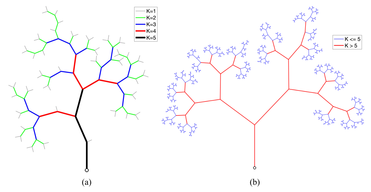
This is a very flexible model that can account for a variety of dendritic patterns. Figure 14 shows four selected examples:
| Fig. 14(a) | ||||
| Fig. 14(b) | ||||
| Fig. 14(c) | ||||
| Fig. 14(d) |
The case corresponds to perfect binary trees with no side branching (see also Ex. 1). In this case, all branch mergers lead to increase of branch order by unity. This results in a most symmetric deterministic tree structure. Some side branching appears for (hence ): every branch of order has on average a single side branch of order , and no side branches of lower orders. This destroys symmetry and introduce randomness in tree shape. The case corresponds to an average of one side branch of any order within a branch of order , resulting in tentacle-shaped formations of varying length. The most complicated case illustrated here corresponds to , which is the Tokunaga sequence for critical binary Galton-Watson trees (but not necessarily vice versa); see Ex. 2. In this case the number of side branches increases geometrically with the difference of branch orders, hence producing branches with widely varying lengths and shapes.
Example 6 (Tokunaga trees with i.i.d. exponential edge lengths).
Random edge lengths often appear as an element of applied modeling. Figure 15 illustrates the same four Tokunaga models as in Ex. 5, with i.i.d. exponential edge lengths. Clearly, this additional random element substantially affects the tree outlook. The edge length variability becomes a dominant element of the metric tree shape. We notice, in particular, that the four types of trees with exponential edge lengths in Fig. 15 look much more similar that the same four types with deterministic edge lengths related to branch order.
Example 7 (Critical Tokunaga processes).
Section 6.5 introduces a subclass of HBP, called critical Tokunaga processes, with , for an arbitrary . These processes generate tree distributions that are Horton self-similar with and have i.i.d. exponential edge lengths.

Example 8 (Independent random attachment).
A variety of mean Horton self-similar measures on can be constructed for an arbitrary sequence of Tokunaga coefficients . Here we give a natural example [81].
Fix a sequence of Tokunaga coefficients. By Remark 5, it is sufficient to construct a set of Horton self-similar conditional measures , .
The subspace , which consists of a single-leaf tree , possesses a trivial unity mass conditional measure . To construct a random tree from , we select a discrete probability distribution , , with the mean value . A random tree is obtained from the single-leaf tree via the following two operations. First, we attach two offspring vertices to the leaf of . This creates a tree of order with no side-branches – one internal vertex of degree 3, two leaves, and the root. Second, we draw the number from the distribution , and attach vertices to this tree so that they form side-branches of index .
In general, we use a recursive construction procedure. Assume that a measure , , is constructed. To construct a random tree we select a set of discrete probability distributions , , on with the respective mean values . A random tree is constructed by adding branches of order (leaves) to a random tree . First, we add two new child vertices to every leaf of hence producing a tree of order with no side-branches of order . Second, for each branch of order in we draw a random number from the distribution and attach new child vertices to this branch so that they form side-branches of index . Each new vertex is attached in a random order with respect to the existing side-branches. Specifically, we notice that side-branches attached to a branch of order are uniquely associated with edges within this branch. The attachment of the new vertices among the edges is given by the equiprobable multinomial distribution with categories and trials.
The procedure described above generates a set of mean-coordinated measures on , since the mean values of the distributions are independent of . Furthermore, observe that
| (26) | |||||
and hence , so the tree is mean self-similar, according to Def. 14.
Finally, to make that construction combinatorially Horton self-similar (Def. 10), each tree must be assigned the probability .
Example 9 (Why coordination?).
Relating mean Horton self-similarity (Def. 16) to mean prune-invariance (Def. 15) is quite intuitive (see also [29]). Much less so is the requirement of mean coordination of conditional measures (Def. 12), included in the definition of mean self-similarity. This requirement is motivated by our goal to bridge the measure-theoretic definition of self-similarity via the pruning operation (Def. 16) to a branch counting definition (Def. 14). In applications, when a handful of trees of different orders is observed, the coordination assumption allows one to estimate the Tokunaga coefficients and make inference regarding the Toeplitz property; see [113, 108, 38, 155]. The absence of coordination, at the same time, allows for a variety of prune-invariant measures with no Toeplitz constraint, which are hardly treatable in applications. To give an example of such a measure, let select any tree from the pre-image of the only tree of order under the pruning operation: . In a similar fashion, select any tree from the pre-image of for . This gives us a collection of trees , such that . Assign the full measure on to : . By construction, the measures are mean prune-invariant. They, however, may satisfy neither the mean coordination nor the Toeplitz property. This example illustrates how one can produce rather obscure collections of mean prune-invariant measures, providing a motivation for the coordination requirement.
4 Horton law in self-similar trees
In this section, we introduce the strong Horton law for the numbers of branches of different orders in a combinatorial tree on (Def. 18) and for the respective averages (Def. 19). The main result of this section (Thm. 1) shows that the mean Horton self-similarity (Defs. 14 and 16) implies the strong Horton law for mean branch numbers (Def. 19).
Consider a measure on and its conditional measures , each defined on subspace of trees of Horton-Strahler order . We write for a random tree drawn from subspace according to measure .
Definition 18 (Strong Horton law for branch numbers).
We say that a probability measure on satisfies a strong Horton law for branch numbers if there exists such a positive (constant) Horton exponent that for any
| (27) |
that is, for any
| (28) |
Corollary 6 in Sect. 6.6.2 is an example of the strong Horton law for branch numbers. In the context of Horton laws, the adjective strong refers to the type of geometric decay, while the convergence of random variables is in probability. Section 4.2 discusses weaker types of geometric convergence. An alternative, weaker, definition of the Horton law is formulated in terms of expected branch counts.
Definition 19 (Strong Horton law for mean branch numbers).
We say that a probability measure on satisfies a strong Horton law for mean branch numbers if there exists such a positive (constant) Horton exponent that for any
| (29) |
Lemma 1.
Proof.
A similar calculation allows us to establish the following result.
Lemma 2.
Sufficient conditions for the strong Horton law for mean branch numbers in binary trees were found in [81], hence providing rigorous foundations for the celebrated regularity that has escaped a formal explanation for a long time. These conditions are presented in Thm. 1 of this section. It has been shown in [82] that the tree that describes a trajectory of Kingman’s coalescent process with particles obeys a weaker version of Horton law as (Sect. 8), and that the first pruning of this tree for any finite is equivalent to a level set tree of a white noise (see Sect. 7 for definitions).
Consider a mean self-similar measure on with a Tokunaga sequence . Define a sequence as
| (30) |
and let denote the generating function of :
| (31) |
For a holomorphic function represented by a power series in a nonempty disk we write
| (32) |
Theorem 1 (Strong Horton law in a mean self-similar tree).
Suppose is a mean Horton self-similar measure on with a Tokunaga sequence such that
| (33) |
Then the strong Horton law for mean branch numbers (Def. 19) holds with the Horton exponent , where is the only real zero of the generating function in the interval . Moreover,
| (34) |
and
| (35) |
Conversely, if , then the limit does not exist at least for some .
That the Horton exponent is reciprocal to the real root of was noticed by Peckham [113], under the assumption .


Below we give two examples of using Theorem 1.
Example 10 (Tokunaga self-similar trees).
Consider a Tokunaga self-similar tree (Def. 17) with , where . (We exclude the case , which correspond to perfect binary trees with no side branching.) This model received considerable attention in the literature [113, 133, 98], in part because of its ability to closely describe river networks [155]. Here we have
and
| (36) | |||||
The discriminant of the quadratic polynomial in the numerator is positive,
Therefore, there exist two real roots, , of the numerator. It is easy to check that
Hence, there is a single root of for of algebraic multiplicity one:
and the respective Horton exponent is
| (37) |
as was observed in earlier works [133, 113, 98]. A map of the values of the Horton exponent is shown in Fig. 16a. As suggested by (37), the level sets of are fairly approximated by
To examine the rate of convergence in the strong Horton law, we use (34). The reciprocal generating function is given by
| (38) | |||||
Thus, since for , formula (34) implies
| (39) | |||||
Accordingly, the rate of convergence in (35) is determined by the ratio – values farther away from 1 lead to faster convergence. Recall (Prop. 3) that
Hence, the ratio also determines the rate of convergence in (29). Figure 16(b) shows the ratio as a function of . The only region when the ratio is approaching 1, hence slowing down the convergence rate in the strong Horton law, corresponds to .

Figure 17 illustrates the strong Horton law in a Tokunaga mean self-similar tree with , which corresponds to , . In this case (Figs. 17(a),18)
| (40) |
The ratios for are shown in Fig. 17(b). The ratios are very close to the theoretical value , except for the branch orders close to the tree order , . As suggested by Fig. 16(b), for most of the choices the convergence rate is higher, so we expect to have a larger number of ratios in a close vicinity of the limit value . As we discussed above, the convergence in (35) has the same rate, with first terms (small ) deviating from the limit value rather then the last ones, as was the case in (29) and Fig. 17(b).
We show below in Eq. 47 that, in general, the rate of convergence in the strong Horton law (29), (35) is controlled by
where separates from other possible zeros of – higher values lead to faster convergence. Figure 18 shows the value on its disk on convergence for the Tokunaga tree of this example. Here, the only zero of at (downward peak) is well isolated so that the surrounding values are separated from zero; this suggests a high rate of convergence that we already illustrated more directly in (39) and Figs. 16(b),17(b).
Example 11 (Shallow side-branching).
Suppose for , that is we only have “shallow” side-branches of orders and . Then
The only root of this equation within is
which leads to
In particular, if for , then ; such trees are called “cyclic” [113]. This shows that the entire range of Horton exponents can be achieved by trees with only very shallow side-branching.
We conclude this section with a linear algebra construction that clarifies the essence of Horton law in a mean self-similar tree. Define a vector of average Horton numbers and a respective normalized vector as
and consider an infinite dimensional extension to operator of (23):
| (41) |
Using these notations, the main counting equations (24) becomes and therefore
Here as , and hence the strong Horton law for mean branch numbers (Def. 19) is equivalent to the existence of a limit solution to an infinite dimensional linear operator equation
with coordinates .
4.1 Proof of Theorem 1
First, we establish (Prop. 4) necessary and sufficient conditions for the existence of the strong Horton law. Then we show that these conditions are satisfied and express the value of the Horton exponent via the Tokunaga coefficients .
Proposition 4.
Let be a mean Horton self-similar measure on . Suppose that the limit
| (42) |
exists and is finite. Then, the strong Horton law for mean branch numbers holds; that is, for each positive integer ,
| (43) |
Conversely, if the limit (42) does not exist, then the limit in the left hand side of (43) also does not exist, at least for some .
Proof.
Next, we express via the elements of the Tokunaga sequence that satisfy condition (33). The quantity can be computed by counting, and expressed via convolution products as follows:
where is the Kronecker delta, and therefore, . Hence, taking the -transform of , we obtain
| (44) |
for small enough. Recalling the definition (32) establishes (34):
Since for any , the function has a single real root in the interval . Our goal is to show that the Horton exponent is reciprocal to . We begin by showing that is the root of closest to the origin.
Lemma 3.
Let be the only real root of in the interval . Then, for any other root of , we have
Proof.
Since are all nonnegative reals, we have . The radius of convergence of must be greater than . Suppose () is a root of magnitude at most . That is and Then and
If , then
arriving to a contradiction. Thus .
Next we show that . Suppose not. Then
arriving to another contradiction. Hence , , and . ∎
Let . Then is the radius of convergence of (we set if ), and Lemma 3 asserts that there exists a positive real such that
| (45) |
Accordingly, for
| (46) |
Observe that is a constant multiple of since is a root of of algebraic multiplicity one. Thus, since and
| (47) |
we have
Proposition 4 now implies the following lemma.
Lemma 4.
Suppose . Then, for each positive integer
Moreover,
To establish the converse we need the following statement.
Proposition 5.
Suppose is a mean Horton self-similar measure on with Tokunaga sequence . Then
for all and
Proof.
Fix any . The main counting equations (22) show that for any integer
Accordingly,
given . Choosing we obtain
∎
Suppose the limit
exists and is finite. Proposition 5 asserts that for all and . Hence,
We summarize this in a lemma.
Lemma 5.
Suppose . Then, the limit does not exist at least for some .
4.2 Well-defined asymptotic Horton ratios
The setting for Horton law in (27) and (29) can be generalized beyond randomizing the tree measure with respect to Horton-Strahler orders as in (7). For instance, as it will be the case with the combinatorial critical binary Galton-Watson trees in (63), the tree measure may be randomized with respect to the number of leaves in a tree. A general set up for the Horton laws is described below.
Let , , be a sequence of probability measures on . We write for the number of branches of Horton-Strahler order in a tree generated according to .
Definition 20 (Well-defined asymptotic Horton ratios).
We say that a sequence of probability measures has well-defined asymptotic Horton ratios if for each
| (48) |
where is a constant, called the asymptotic Horton ratio of the branches of order .
Sometimes it is possible to establish a stronger limit than in (48). One such example is the almost sure convergence in equation (130) of Sect. 6.6.2.
For a sequence of well-defined asymptotic Horton ratios , the Horton law states that decreases in a geometric fashion as goes to infinity. We consider three particular forms of geometric decay.
Definition 21 (Root, ratio, and strong Horton laws).
Consider a sequence of probability measures on with well-defined asymptotic Horton ratios (Def. 20). Then, the sequence is said to obey
- •
a root-Horton law if the following limit exists: ;
- •
a ratio-Horton law if the following limit exists: ;
- •
a strong Horton law if the following limit exists: .
The constant is called the Horton exponent. In each case, we require the Horton exponent to be finite and positive.
Observe that the Horton laws in Def. 21 above are listed in the order from weaker to stronger.
4.3 Entropy and information theory
The information theoretical aspects of self-similar trees were not addressed until very recently. This section reviews recent results by Chunikhina [33, 34], where the entropy rate is computed for trees that satisfy the strong Horton law for branch numbers (Def. 18) and for Tokunaga self-similar trees (Def. 17) as a function of the respective parameters, and .
Consider a subspace of of trees of a given order and given admissible (, ) branch counts :
In [33], Chunikhina finds the size of , providing an alternative form of expression that was first derived by Shreve [124].
Lemma 6 (Branch counting lemma, [33]).
Subsequently, Lem. 6 is used to find the entropy rate for trees that satisfy the strong Horton law (Def. 18) with exponent .
Theorem 2 (Entropy rate for Horton self-similar trees, [33]).
Notice that the trees in satisfy the strong Horton law (Def. 18) with the Horton exponent , and is the asymptotic number of nodes in a tree from .
Remark 7.
It is an easily verified fact that a random tree selected uniformly from the subspace
| (51) |
of containing only the trees with leaves ( nodes and edges) is distributed as a random tree sampled from the critical plane Galton-Watson distribution , conditioned on , i.e.,
| (52) |
Consequently, we have that
| (53) |
The number of different combinatorial shapes of rooted planted plane binary trees with leaves and edges, is given by , where denotes the Catalan number defined as
| (54) |
Using and Stirling’s formula, it is observed in [33] that the entropy rate for a tree , selected uniformly from is
| (55) |
Thus, scaling by the asymptotic number of nodes in Thm. 2 implies
Indeed, by definition of the corresponding spaces,
where the union is taken over ranging from
and therefore
Hence, for the following limits known to converge, we have
Moreover, scaling by the asymptotic number of nodes in Thm. 2 enables representing as the limit ratio of the entropy for Horton self-similar trees with parameter to the entropy for uniformly selected binary trees. Specifically, let be a random tree sampled uniformly from the space and let be a random tree sampled uniformly from the space with . Then, equations (49) and (55) imply that is the the limit ratio of entropies as the space sizes grow with :
| (56) |
As an important consequence of Thm. 2, a special place of the parameter is established amongst all Horton exponents as
Not surprisingly, is the parameter value for the strong Horton law results we will encounter in Sect. 5, primarily in the context of the critical binary Galton-Watson tree . Indeed, as stated in Rem. 7, the tree in (56) is a random tree sampled from the Galton-Watson distribution conditioned on .
In [34], Chunikhina extended the results in [33] by counting the number of trees with the given merger numbers (see Sect. 3.3), and finding the entropy rates for the Tokunaga self-similar trees (Def. 17) represented as a function of the parameters . For a given integer , consider a finite sequence of admissible branch counts , and a finite sequence of admissible branch numbers . Admissibility means that for all ,
as all branches of Horton-Strahler order have to merge into a higher order branch (either two branches of order merge and originate a branch of order , or a branch of order merges into a branch of order ). Consider the subspace
Lemma 7 (Side branch counting lemma, [34]).
Lemma 7 is used to obtain the following asymptotic results. Consider Tokunaga self-similar tree with parameters . Such a tree satisfies the strong Horton law for mean branch numbers (Def. 19) with the Horton exponent (37)
Next, similarly to , one can define the space of asymptotically Tokunaga self-similar trees of order . Informally, this space includes the trees in such that
where , and the asymptotic equality is taken as .
Theorem 3 (Entropy rate for Tokunaga self-similar trees, [34]).
For given , let be a random tree, uniformly sampled from the space . Then, the entropy rate
| (57) |
Figure 20(a) illustrates the entropy rate .

Corollary 1 ([34]).
Figure 20(b) illustrates this result, by showing how the difference of entropy rates decreases away from the line . The special place for the line within the parameter space of the Tokunaga self-similar random trees was observed earlier in [139, 83, 84]. See Remark 11. The constraint will reappear in many instances in Sect. 6 of the present work.
Finally, the maximum value is achieved at the special point of the special line . Once again, this is not surprising as is the parameter value for the Tokunaga self-similarity results of Sect. 5, presented in the context of the critical binary Galton-Watson trees and related processes. We recall that the combinatorial shape of the random binary tree in (55) is distributed according to conditioned on .
4.4 Applications
A quantitative understanding of the branching patterns is instrumental in hydrology [120, 132, 96, 15, 27, 76], geomorphology [38, 67], statistical seismology [13, 135, 69, 154, 60, 151, 149], statistical physics of fracture [121], vascular analysis [72], brain studies [32], ecology [30], biology [137], and beyond, encouraging a rigorous treatment. Introduced in hydrology to describe the dendritic structure of river networks, which is among the most evident examples of natural branching, Horton-Strahler [70, 129] and Tokunaga [133] indexing schemes have been rediscovered and used in other fields. Subsequently, the Horton law (Def. 18) and Tokunaga self-similarities (Def. 17) have been empirically or rigorously established in numerous observed and modeled systems [108]. This includes hydrology (see Sect. 4.4.1), vein structure of botanical leaves [108, 137], diffusion limited aggregation [111, 97, 147], two dimensional site percolation [136, 145, 152, 153], a hierarchical coagulation model of Gabrielov et al. [58] introduced in the framework of self-organized criticality, and a random self-similar network model of Veitzer and Gupta [139] developed as an alternative to the Shreve’s random topology model for river networks. The Horton exponent commonly reported in empirical studies is within the range . Curiously, it has been observed in [83] that the critical Tokunaga model (Sect. 6.5) with this range of Horton exponents generates trees with fractal dimension in the range , which includes all the trees that may exist in a three-dimensional world, excluding the range that corresponds to almost “linear”, and probably less studied, trees.
4.4.1 Hydrology
An illuminating natural example of Horton laws and Tokunaga self-similarity is given by the combinatorial structure of river networks (Figs. 2,3). The hydrological Horton law was first described by Robert E. Horton [70] who noticed that the empirical ratio in river streams is close to . This observation has been strongly corroborated in numerous observational studies [75, 124, 91, 113, 131, 62, 120, 101, 134]. See Barndorff-Nielsen [17] for a 1993 survey for probabilists.
Write for the value of a selected statistic averaged over basins/channels of order . This can be basin area, basin magnitude (number of leaves in the tree that describes the basin), the lengths of the longest channel, the total channel lengths, etc. The Horton law approximates the growth of with order as a geometric sequence: with . Informally, this suggests that the order of a channel (branch) or a subbasin (subtree) is proportional to , where can be interpreted as the channel/basin “size”. If statistic satisfies the Horton law with exponent , and the branch counts satisfy the Horton law (1) with Horton exponent , then
A similar power relation holds for any pair of statistics that satisfy the Horton law. A well studied example is the Hack’s law that relates the length of the longest stream to the basin area via with [119].
Furthermore, it has been shown that river networks are closely approximated by a two-parametric Tokunaga self-similar model (Def. 17) with parameters that are independent of river’s geographic location [133, 113, 38, 155]. The Tokunaga model closely predicts values of the Horton exponents for multiple basin statistics with only two parameters (see Fig. 3).
Discovery of the Horton law prompted exploration of various branching models, most popular of which is the critical binary Galton-Watson tree (Sect. 5), also known in hydrology as Shreve’s random topology model [124, 125]; it is conditionally equivalent to the uniform distribution on planar binary trees with a fixed number of leaves [116]. This model has the Horton exponent and Tokunaga parameters ; see Thm. 4. For long time, the critical binary Galton-Watson tree has remained the only well-known probability model for which the Horton and Tokunaga self-similarity was rigorously established, and whose Horton-Strahler ordering has received attention in the literature [124, 125, 73, 17, 36, 113, 112, 143, 148, 29]. The model has been particularly popular in hydrology as an approximation to the topology of the observed river networks [132]. Scott Peckham [113] has first explicitly noticed, by performing a high-precision extraction of river channels for Kentucky River, Kentucky and Powder River, Wyoming, that the Horton exponents and Tokunaga parameters for the observed rivers significantly deviate from that for the Galton-Watson model. He reported values and and emphasized the importance of studying a broad range of Horton exponents and Tokunaga parameters. The general interest to fractals and self-similar structures in natural sciences during the s resulted in a quest, mainly inspired and led by Donald Turcotte, for Tokunaga self-similar tree graphs of diverse origin. As a result, the Horton and Tokunaga self-similarity, with a broad range of respective parameters, have been empirically or rigorously established in numerous observed and modeled systems, well beyond river networks.
4.4.2 Computer science
The Horton-Strahler orders are known in computer science as the register function or register number. They first appeared in the paper by Ershov [49] as the minimal number of memory registers required for evaluating a binary arithmetic expression.
A study of Flajolet et al. [55] concerns calculating the average register function in a random plane planted binary tree with leaves. That is, let the random tree be uniformly sampled from all trees in the subspace of defined in (51), where is the Catalan number (54). Following Rem. 7, we know that the combinatorial shape of such binary tree can also be obtained by sampling from the Galton-Watson distribution conditioned on . The work [55] finds the average register function (Horton-Strahler order) in a random binary tree ,
where is known as the dyadic valuation of . Specifically, the dyadic valuation of is the cardinality of the inverse image of
i.e., .
In addition, Flajolet et al. [55] proved that for ,
| (59) |
where is a particular continuous periodic function of period one, explicitly derived in [55]. We illustrate Eq. (59) below in Fig. 50(a), which closely reproduces Fig. 6 from the original paper by Flajolet et al. [55]. Equation (59) is related to the tree size asymptotic (35) of Thm. 1, with the Horton exponent .
5 Critical binary Galton-Watson tree
The critical binary Galton-Watson tree is pivotal for the theory of random trees and for diverse applications because of its transparent generation process and multiple symmetries. This section summarizes some properties of this tree used in our further discussion.
5.1 Combinatorial case
Here we discuss the combinatorial binary Galton-Watson trees.
5.1.1 Horton and Tokunaga self-similarities
Burd, Waymire, and Winn [29] have first recognized a special position held by the critical binary tree with respect to the Horton pruning in the space of Galton-Watson distributions on . We now state the main result of [29] using the language of the present work.
Theorem 4 (Horton self-similarity of Galton-Watson trees, [29]).
Consider a collection of Galton-Watson measures on . The following statements are equivalent:
- (a)
A distribution is Horton self-similar (Def. 10);
- (b)
- (c)
A distribution is Tokunaga self-similar (Def. 17);
- (d)
A distribution is critical binary: .
Furthermore, the critical binary distribution has Tokunaga sequence , , which corresponds to Tokunaga self-similarity with and strong Horton law with exponent .
The following statement provides a useful characterization of the critical binary Galton-Watson tree.
Proposition 6 ([29]).
Suppose . Then, the tree order has geometric distribution:
Furthermore, let be a branch of order in selected uniformly and randomly among all branches of order in . Then, the total number of side branches within the branch is geometrically distributed:
In particular,
where , , are the Tokunaga coefficients. Conditioned on , each side branch within is assigned order independently of other side branches with probability
Notably, critical non-binary Galton-Watson trees converge to the critical binary tree under consecutive Horton pruning, as described in the following statement.
Theorem 5 (Attraction property of critical binary Galton-Watson tree, [29]).
Suppose a Galton-Watson measure on satisfies the following conditions:
- •
The measure is critical, i.e. and ;
- •
The measure has a.s. bounded offspring number, i.e. there exists such that for any .
Then, for any
where denotes the critical binary Galton-Watson measure on :
| (60) |
The Markov structure of the Galton-Watson tree ensures the existence of the following additional properties:
- (i)
The forest of trees obtained by removing the edges and the vertices below combinatorial depth has the same frequency structure as the original space ;
- (ii)
A subtree rooted in a uniform random vertex of has the same distribution as ; and
- (iii)
The forest of trees obtained by considering subtrees rooted at every vertex of approximates the frequency structure of the entire space of trees when the order of increases.
We define these properties more formally in Sect. 6.7. Combined with the Horton self-similarity of Thm. 4, they further highlight very special symmetries of the critical binary Galton-Watson distribution . Stated loosely, this distribution is invariant with respect to various form of cutting, either from the leaves down or from the root up. Moreover, this is the only distribution that enjoys all these invariances in the family of Galton-Watson distributions . Analysis of real world data (e.g. [113, 108]), however, reveals self-similar tree-like structures with Tokunaga parameters and Horton exponents different from those in the critical binary Galton-Watson model. This motivates one to look for invariant tree models outside of the Galton-Watson family. In Sect. 6.5, we construct a one parameter family of trees, called critical Tokunaga trees, that inherit all the invariant properties mentioned in this section and include the critical binary Galton-Watson tree as a special case. In particular, it generates self-similar trees with Horton exponents .
5.1.2 Dynamics of branching probabilities under Horton pruning
The following result of Burd et al. [29] clarifies the Horton self-similarity of the critical binary Galton-Watson tree and absence of such in non-critical case.
Theorem 6 (Dynamics of branching [29, Proposition 2.1]).
Consider a critical or subcritical combinatorial binary Galton-Watson probability measure on , i.e. require and . Construct a recursion by repeatedly applying Horton pruning operation as follows. Starting with , and for each consecutive integer, let be the pushforward probability measure induced by the pruning operator, i.e.,
and set
Then for each , distribution is a binary Galton-Watson distribution with and constructed recursively as follows: start with and , and let
| (61) |
Consequently, a combinatorial binary Galton-Watson probability distribution is prune-invariant as in the Def. 8 if and only if it is critical, i.e.,
5.1.3 The Central Limit Theorem and the strong Horton law for branch counts
For a given , consider . Following Remark 7, we know that . The branch counts
are integer valued random variables induced by . They are the same for and , i.e., . The following Law of Large Numbers was proved in Wang and Waymire [143] (Theorem 2.1).
Theorem 7 (LLN for order two branches, [143]).
For a random tree ,
| (62) |
Recall that we know from Theorem 6 that the critical binary Galton-Watson tree is invariant under the Horton pruning operation . Thus, the strong Horton law for branch numbers is deduced from Theorem 7 as follows.
Corollary 2 (The strong Horton law for branch counts).
For a random tree and for all ,
| (63) |
Proof.
For a fixed integer and a tree , we have for any positive integers and ,
| (64) | ||||
as by the Horton prune-invariance Theorem 6 (and a more general statement in Theorem 24 of Sect. 9.4). The first equality in (64) can be easily verified from permutability of attachments of smaller order branches to the larger order branches. Specifically, the event is equivalent to the event that the pruned tree will have edges. Thus, conditioned of the combinatorial shape , all complete subtrees (see Def. 5(6)) of such that and will be attached to the edges and leaves of in the same number of ways, for each satisfying edges.
Following Theorem 7, the corresponding Central Limit Theorem was proved in Wang and Waymire [143] (Theorem 2.4).
Theorem 8 (CLT for order two branches, [143]).
For a random tree ,
| (66) |
Next, using the pruning framework, the following Central Limit Theorem for is readily obtained as a direct consequence of the original Theorem 8 of Wang and Waymire [143] and the Horton prune-invariance (Def. 8) of as stated in Theorem 6, and a more general statement that will appear in Theorem 24 of Sect. 9.4.
Corollary 3 (CLT for branch numbers, [146]).
For a random tree ,
| (67) |
where we set .
Proof.
5.2 Metric case
In this section we turn to the trees in . In particular, we will assign i.i.d. exponential lengths to the edges of a critical plane binary Galton-Watson tree in , thus obtaining what will be called the exponential critical binary Galton-Watson tree.
Definition 22 (Exponential critical binary Galton-Watson tree).
We say that a random tree is an exponential critical binary Galton-Watson tree with (edge length) parameter , and write , if the following conditions are satisfied:
- (i)
p-shape() is a critical plane binary Galton-Watson tree ;
- (ii)
conditioned on a given p-shape(), the edges of are sampled as independent random variables, i.e., random variables with probability density function (p.d.f.)
(69)
The branching process that generates an exponential critical binary Galton-Watson tree is known as the continuous time Galton-Watson process, and is sometimes simply called Markov branching process [66].
5.2.1 Length of a Galton-Watson random tree
Recall the modified Bessel functions of the first kind
Lemma 8.
Suppose is an exponential critical binary Galton-Watson tree with parameter . The total length of the tree has the p.d.f.
| (70) |
Proof.
Recall that the number of different combinatorial shapes of a planted plane binary tree with leaves, and therefore edges, is given by the Catalan number (54), i.e.,
The total length of edges is a gamma random variable with parameters and and density function
Hence, the total length of the tree has the p.d.f.
| (71) |
∎
Next, we compute the Laplace transform of . By the summation formula in (5.2.1),
where we let , and the characteristic function of Catalan numbers
| (72) |
is well known. Therefore
| (73) |
Note that the Laplace transform could be derived from the total probability formula
| (74) |
where is the exponential p.d.f. (69). Thus, solves
| (75) |
Corollary 4.
The p.d.f. of the length of an excursion in an exponential symmetric random walk with parameter is given by
| (76) |
Proof.
Observe that the excursion has twice the length of a tree . ∎
5.2.2 Height of a Galton-Watson random tree
Lemma 9 ([85]).
Suppose is an exponential critical binary Galton-Watson tree with parameter . Then, the height of the tree has the cumulative distribution function
| (77) |
Proof.
The proof is based on duality between trees and positive real excursions that we introduce in Sect. 7. In particular, Thm. 18 establishes equivalence between the level set tree (Sect. 7.2) of a positive excursion of an exponential random walk (Sect. 7.6) and an exponential critical binary Galton-Watson tree . This implies, in particular, that for a tree the has the same distribution as the height of a positive excursion of an exponential random walk with and independent increments distributed according to the Laplace density function , with defined in (69).
Notice that is a martingale. We condition on , and consider an excursion with denoting the termination step of the excursion. For , we write
for the probability that the height of the excursion exceeds . The problem of finding is solved using the Optional Stopping Theorem. Let
Observe that
For a fixed , by the Optional Stopping Theorem, we have
Hence,
Thus,
and therefore,
Hence,
∎
We continue examining the height function for . This time, we condition on , i.e., the tree has leaves and internal non-root vertices. We let denote the corresponding conditional cumulative distribution function,
| (78) |
There, for a one-leaf tree,
| (79) |
and for , the following recursion follows from conditioning on the length of the stem (root edge),
| (80) |
where is the Catalan number as defined in (54).
Next, we consider the following -transform:
| (81) |
which, if we let , simplifies to
We differentiate the above equation, obtaining
| (82) |
Let
be the two roots of . Here, is the -transform of the Catalan sequence , introduced in (72). Then, (82) solves as
where due to the initial conditions , we have , and
| (83) |
Solution (83) implies
| (84) |
Here and throughout we use branch of the logarithm when defining for .
Now, since , the series expansion (81) implies
| (85) |
where is real. We substitute (84) into the limit (85),
| (86) |
thus obtaining an alternative proof of formula (77) in Lemma 9.
The asymptotic of the height distribution for a given number of leaves was the object of analysis in [79, 144, 61, 44]. In particular, Gupta et al. [61] extended the results of Kolchin [79], by showing that
| (87) |
It was also observed in [61] that is the distribution function for the maximum of the Brownian excursion as shown in the work of Durrett and Iglehart [43]. The results of [61] were further developed in [44] for more general trees with edge lengths.
6 Hierarchical Branching Process
Tree self-similarity has been studied primarily in terms of the average values of selected branch statistics, as defined in Sect. 3.3. Until recently, the only rigorous results have been obtained only for a very special classes of Markov trees (e.g., binary Galton-Watson trees with no edge lengths, as in Sect. 5.1). At the same time, solid empirical evidence motivates a search for a flexible class of self-similar models that would encompass a variety of observed combinatorial and metric structures and rules of tree growth. In Sec. 3.2 we introduced a general concept of self-similarity that accounts for both combinatorial and metric tree structure. In this section we will describe a model called hierarchical branching process that generates a broad range of self-similar trees (Thm. 9) and includes the critical binary Galton-Watson tree with exponential edge lengths as a special case (Thm. 13). We will also introduce a class of critical self-similar Tokunaga processes (Sect. 6.5) that enjoy additional symmetries — their edge lengths are i.i.d. random variables (Prop. 10), and subtrees of large Tokunaga trees reproduce the probabilistic structure of the entire random tree space (Prop. 11). The results of this section are derived in [84].
The results of Sect. 5 concerned a very narrow class of mean self-similar trees with . Among such trees, the self-similarity is established only for the critical binary Galton-Watson tree with independent exponential edge lengths, i.e., continuous parameter Galton-Watson binary branching Markov processes; this case corresponds to the scaling exponent . Next, we construct a multi-type branching process [66, 11] that generates self-similar trees for an arbitrary sequence and for any ; it includes the critical binary Galton-Watson tree as a special case.
6.1 Definition and main properties
Consider a probability mass function , a sequence of nonnegative Tokunaga coefficients, and a sequence of positive termination rates. We now define a hierarchical branching process .
Definition 23 (Hierarchical Branching Process (HBP)).
We say that is a hierarchical branching process with a triplet of parameter sequences , , and , and write
if is a multi-type branching process that develops in continuous time according to the following rules:
- (i)
The process starts at with a single progenitor (root branch) whose Horton-Strahler order (type) is with probability .
- (ii)
Every branch of order produces offspring (side branches) of every order with rate . Each offspring (side branch) is assigned a uniform random orientation (right or left).
- (iii)
A branch of order terminates with rate .
- (iv)
At its termination time, a branch of order splits into two independent branches of order . The two branches are assigned uniform random orientations, i.e., a uniformly randomly selected branch becomes right and the other becomes left.
- (v)
A branch of order terminates without leaving offspring.
- (vi)
Generation of side branches and termination of distinct branches are independent.
The definition implies that the process terminates a.s. in finite time. Accordingly, the branching history of creates a random binary tree in the space of planted binary trees with edge lengths and planar embedding. To avoid heavy notations, we sometimes use the process distribution name , as well as its various special cases introduced below, to also denote the measures induced by the process on suitable tree spaces (, , etc.)
The next statement describes the branching structure of .
Proposition 7 (Side-branching in hierarchical branching process, [84]).
Consider a hierarchical branching process and let be the tree generated by in . For a branch of order , let be the number of its side branches of order , and be the total number of the side branches. Conditioned on , let be the lengths of edges within , counted sequentially from the initial vertex, and be the total branch length. Define
for by assuming . Then the following statements hold:
- 1.
The tree order satisfies
(88) - 2.
The total number of side branches within a branch of order has geometric distribution:
(89) with
- 3.
Conditioned on the total number of side branches, the distribution of vector is multinomial with trials and success probabilities
(90) The vector of side branch orders, where the side branches are labeled sequentially starting from the initial vertex of , is obtained from the sequence
by a uniform random permutation of indices :
- 4.
The total numbers of side branches and orders of side branches are independent in distinct branches.
- 5.
The branch length has exponential distribution with rate , independent of the lengths of any other branch (of any order). The corresponding edge lengths are i.i.d. random variables; they have a common exponential distribution with rate
(91)
Proof.
All the properties readily follow from Def. 23. ∎
Combining properties 2 and 3 of Prop. 7 we find that the number of side branches of order within a branch of order has geometric distribution:
| (92) |
with We also notice that the numbers for within the same branch are dependent.
Proposition 7 provides an alternative definition of the hierarchical branching process and suggests a recursive construction of that does not require time-dependent simulations. Specifically, a tree of order consists of two vertices (root and leaf) connected by an edge of exponential length with rate . Assume now that we know how to construct a random tree of any order below . To construct a tree of order , we start with a perfect (combinatorial) planted binary tree of depth , which we call skeleton. The combinatorial shapes of such trees is illustrated in Fig. 13. All leaves in the skeleton have the same depth , and all vertices at depth have the same Horton-Strahler order . The root (at depth 0) has order . Next, we assign lengths to the branches of the skeleton. Recall (Ex. 1) that each branch in a perfect tree consists of a single edge. To assign length to a branch of order , with , we generate a geometric number according to (89) and then i.i.d. exponential lengths , , with the common rate according to (91). The total length of the branch is . Moreover, branch has side branches that are attached along with spacings , starting from the branch point closest to the root. The order assignment for the side branches is done according to (90). We generate side branches (each has order below ) independently and attach them to the branch . This completes the construction of a random tree of order . To construct a random HBP tree, one first generates a random order according to (88) and then constructs a tree of order using the above recursive process.
Next, we establish various forms of self-similarity for the hierarchical branching process.
Theorem 9 (Self-similarity of hierarchical branching process, [84]).
Consider a hierarchical branching process and let be the tree generated by on . The following statements hold.
Proof.
By process construction, the tree is coordinated in shapes and lengths (according to Def. 11), with independent complete subtrees.
(1) Proposition 7, part (3) implies that the expected value of the number of side branches of order within a branch of order is given by . The mean self-similarity of Def. 14 with coefficients immediately follows, using a conditional argument as in (26).
(2) Assume that is self-similar. A geometric distribution of orders is then established in Prop. 1. Inversely, a geometric distribution of orders ensures that the total mass , , is invariant with respect to pruning. The conditional distribution of trees of a given order is completely specified by the side branch distribution, described in Proposition 7, parts (1)-(3). Consider a branch of order , . Pruning decreases the orders of this branch, and all its side branches, by unity. Pruning eliminates a random geometric number of side-branches of order from the branch. It acts as a thinning with removal probability on the total side branch count . Accordingly, the total side branch count after pruning has geometric distribution with success probability
The order assignment among the remaining side branches (with possible orders ) is done according to multinomial distribution with probabilities proportional to . This coincides with the side branch structure in the original tree, hence completing the proof of (2).
(3) Having proven (2), it remains to prove the statement for the length structure of the tree. Assume that is self-similar with scaling exponent . The branches of order become branches of order after pruning, which necessitates . Inversely, pruning acts as a thinning on the side branches within a branch of order , eliminating the side branches of order . Accordingly, the spacings between the remaining side branches are exponentially distributed with a decreased rate
Comparing this with (91), and recalling the self-similarity of , we conclude that Def. 11 is satisfied with scaling exponent . ∎
6.2 Hydrodynamic limit
Here we analyze the average numbers of branches of different orders in a hierarchical branching process, using a hydrodynamic limit. Specifically, let be the number of branches of order at time observed in independent copies of the process . Let be the number of branches of order in the process at instant . We observe that, by the law of large numbers,
Theorem 10 (Hydrodynamic limit for branch dynamics, [84]).
Suppose that the following conditions are satisfied:
| (93) |
and
| (94) |
Then, for any given , the empirical process
converges almost surely, as , to the process
that satisfies
| (95) |
where is a diagonal operator with the entries , are the standard basis vectors, and operator defined in Eq. (41).
Proof.
The process evolves according to the transition rates
with
Here the first term reflects termination of branches of order ; the second term reflects termination of branches of orders , each of which results in creation of two branches of order ; and the last term reflects side-branching. Thus, the infinitesimal generator of the stochastic process is
| (96) | |||||
Let
The convergence result of Kurtz ([50, Theorem 2.1, Chapter 11], [87, Theorem 8.1]) given here in Appendix A extends (without changing the proof) to the Banach space provided the same conditions are satisfied for as for in Theorem 33. Specifically, we require that for a compact set in ,
| (97) |
and there exists such that
| (98) |
Here the condition (97) follows from
which in turn follow from conditions (94). Similarly, Lipschitz conditions (98) are satisfied in due to conditions (94). Thus, by Theorem 33 extended for , the process converges almost surely to that satisfies , which expands as the following system of ordinary differential equations:
| (99) |
with the initial conditions by the law of large numbers. Finally, we observe that , and conditions (94) imply that is a bounded operator in . ∎
6.3 Criticality and time invariance
6.3.1 Definitions
Assume that the hydrodynamic limit , and hence the averages , exist. Write for the initial distribution of the process. Consider the average progeny of the process, that is the average number of branches of any order alive at instant :
Definition 24.
A hierarchical branching process is said to be critical if its average progeny is constant: for all .
Definition 25.
A hierarchical branching process is said to be time-invariant if
| (100) |
Proposition 8.
Suppose the hydrodynamic limit exists, and the hierarchical branching process is time-invariant. Then the process is critical.
Proof.
∎
Recall the function defined in Eq. (31) for all complex , where the inverse radius of convergence is defined in Eq. (93). We also recall that there is a unique real root of within . We formulate some of the results below in terms of and the Horton exponent ; see Theorem 1.
Proposition 9.
Suppose is a constant multiple of the geometric vector . Then the process is time-invariant.
Proof.
Observe that since and is a Toeplitz operator,
and
Hence and
∎
Remark 8.
Proposition 9 states that the condition
| (101) |
is sufficient for time-invariance, for any proportionality constant . This implies that a time-invariant process can be constructed for
- (i)
an arbitrary sequence of Tokunaga coefficients satisfying (93) – by selecting ;
- (ii)
arbitrary sequences satisfying (93) and – by selecting ;
- (iii)
arbitrary sequences satisfying (93) and – by selecting .
At the same time, arbitrary sequences will not, in general, satisfy (101) and hence will not correspond to a time-invariant process.
6.3.2 Criticality and time-invariance in a self-similar process
A convenient characterization of criticality can be established for self-similar hierarchical branching processes. Recall that by Theorem 9, part (3), a self-similar process is specified by parameters , and length self-similarity constant such that and . We refer to a self-similar process by its parameter triplet, and write . We denote the respective average progeny by . Observe that in the self-similar case the first of the conditions (94) is equivalent to , and the second is equivalent to . Hence, the conditions (94) are equivalent to .
Theorem 11 (Average progeny of a self-similar process, [84]).
Consider a self-similar process with and . Suppose that (93) is satisfied and . Then
Proof.
The choice of the limits for ensures that the conditions (94) are satisfied and hence, by Theorem 10, the hydrodynamic limit exists and the function is well defined. Now we have
and therefore
| (102) |
Iterating recursively, we obtain
and in general,
Thus, taking ,
| (103) |
The average progeny function for fixed values of , and can therefore be expressed as
| (104) |
since
Next, notice that by letting , we have from (6.3.2) and the uniform convergence of the corresponding series for any fixed and , that
| (105) |
Observe that implies and . Also, observe that
as is an increasing function on and . This leads to the statement of the theorem. ∎
Remark 9.
If , then and equation (105) has an explicit solution
Accordingly,
This case is further examined in Sect. 6.4. In general, the average progeny may increase sub-exponentially for . For example, if there is a nonnegative integer such that , then for we have . Accordingly, (103) implies that is a polynomial of degree .
Theorem 12 (Criticality of a self-similar process, [84]).
Consider a self-similar process with , . Suppose that (93) is satisfied and . Then the following conditions are equivalent:
- (i)
The process is critical.
- (ii)
The process is time-invariant.
- (iii)
The following relations hold:
Proof.
Remark 10.
By Thm. 9, the product in a self-similar process is given by
for some , , and . Hence, a time-invariant process can be constructed, according to Prop. 9 and (101), by selecting any sequence such that the unique real zero on of the respective function is given by
Theorem 12 states that this is the only possible way to construct a time-invariant process, given that the process is self-similar.
6.4 Closed form solution for equally distributed branch lengths
Consider a self-similar hierarchical branching process with and for a given integer . In other words, we assume for all , which implies .
In this case, the system of equation (99) is finite dimensional,
| (106) |
with the initial conditions .
Recall the sequence defined in Eq. (30), and let . Then (106) rewrites in terms of the coordinates of as follows
| (107) |
with the initial conditions . The ODEs (107) can be solved recursively in a reversed order of equations in the system obtaining for ,
Let be the Kronecker delta function. Then we arrive with the closed form solution
| (108) |
Observe that if we randomize the orders of trees by assigning an order to a tree with geometric probability , then the above closed form expression (6.4) would yield an expression for the average progeny that was observed in Remark 9 of this section:
6.5 Critical Tokunaga process
We introduce here a class of hierarchical branching processes that enjoy all of the symmetries discussed in this work – Horton self-similarity, criticality, time-invariance, strong Horton law, Tokunaga self-similarity, and also have independently distributed edge lengths. Despite these multiple constraints, the class is sufficiently broad, allowing the self-similarity constant (Def. 11, part (iv)) to take any value , and the Horton exponent to take any value . The critical binary Galton-Watson process is a special case of this class.
Definition 26 (Critical Tokunaga process).
We say that is a critical Tokunaga process with parameters (, ), and write , if it is a hierarchical branching process with the following parameter triplet:
| (109) |
for some .
Proposition 10 (Critical Tokunaga process).
Suppose and let be the tree of . Then,
- 1.
is a Horton self-similar, critical, and time invariant process
- 2.
Independently of the combinatorial shape of , its edge lengths are i.i.d. exponential random variables with rate .
- 3.
We have
Proof.
1. Self-similarity follows from Thm. 9, part (3). Specification of parameters (109) implies and . The Horton exponent is found from (37). Criticality and time-invariance now follow from Thm. 12, since here
2. To establish the edge lengths property, observe that
Recall from Prop. 7, part(4) that the edge lengths within a branch of order are i.i.d. exponential r.v.s with rate
3. The values of , , and are found in 1. The expression for and equality are readily obtained from the geometric form of the Tokunaga coefficients . ∎
Criticality and i.i.d. edge length distribution property characterize the critical Tokunaga process, as we explain in the following statement.
Lemma 10.
Consider a self-similar hierarchical branching process with and . Suppose that (93) holds and . Let be the tree of . Then, the following conditions are equivalent:
- 1.
is critical and the edges in have i.i.d. exponential lengths with rate .
- 2.
is a critical Tokunaga process:
Proof.
The implication () was established in Prop. 10. To show (), recall from Prop. 7, Eq. (91), that the edge lengths within a branch of order are i.i.d. with rate . If the rate is independent of , we have for any :
or
Given , we find , and hence By (37), the Horton exponent is . Criticality implies (Prop. 12, part (iii)):
which completes the proof. ∎
It follows from the proof of Lemma 10 that the i.i.d. edge length property alone (and no criticality) is equivalent to the following constraints on the process parameters:
while allowing an arbitrary choice of . The tree of such process is Tokunaga self-similar, although not critical unless .
The next results shows that the critical binary Galton-Watson tree with i.i.d. exponential edge lengths is a special case of the critical Tokunaga process.
Theorem 13 (Critical binary Galton-Watson tree, [84]).
Suppose is a critical Tokunaga process with parameters
| (110) |
which means . Let be the tree of . Then has the same distribution on as the critical binary Galton-Watson tree with i.i.d. edge lengths: .
Proof.
Consider a tree in . We show below that this tree can be dynamically generated according to Def. 23 of the hierarchical branching process with parameters (110).
First, notice that by Prop. 6
We will establish later in Corollary 12 that the length of every branch of order in is exponentially distributed with parameter , which matches the branch length distribution in the hierarchical branching process (110). Furthermore, by Corollary 12, conditioned on (which happens with a positive probability), we have . This means that the distribution of Galton-Watson trees pruned times is a linearly scaled version of the original distribution (the same combinatorial structure, linearly scaled edge lengths). Recall (Prop. 6) the total number of side branches within a branch of order in is geometrically distributed with mean , where , . Conditioned on , the assignment of orders among the side-branches is done according to the multinomial distribution with trials and success probability for order given by . This implies that the leaves of the original tree merge into every branch of the pruned tree as a Poisson point process with intensity . Iterating this pruning argument, the branches of order merge into any branch of order in the pruned tree as a Poisson point process with intensity for every .
Remark 11.
The condition was first introduced in hydrology by Eiji Tokunaga [133] in a study of river networks, hence the process name. The additional constraint is necessitated here by the self-similarity of tree lengths, which requires the sequence to be geometric. The sequence of the Tokunaga coefficients then also has to be geometric, and satisfy , to ensure identical distribution of the edge lengths, see Prop. 7(4). Recall the special place case plays for the entropy rate of Tokunaga self-similar trees as elaborated in Sect. 4.3. See Cor. 1. Interestingly, the constraint appears in the random self-similar network (RSN) model introduced by Veitzer and Gupta [139], which uses a purely topological algorithm of recursive local replacement of the network generators to construct random self-similar trees. The importance of the constraint in purely combinatorial context is revealed in Sect. 6.7.
6.6 Martingale approach
In this section, we propose a martingale representation for the size and length of a critical Tokunaga tree of a given order. This leads, via the martingale techniques, to the strong Horton laws for both these quantities, and allows us to find the asymptotic order of a tree of a given size. The proposed martingale representation is related to an alternative construction of a critical Tokunaga tree, via a Markov tree process on .
6.6.1 Markov tree process
Consider a critical Tokunaga process (Def. 26) with (hence excluding a trivial case of perfect binary trees), and let be the measure induced by this process on . Following the notations introduced in Sect. 3.1, Eq. (6), we consider conditional measures
Next, we construct a discrete time Markov tree process on such that for each ,
| (111) |
Let
be the number of leaves in and be the tree length. We let be an I-shaped tree of Horton-Strahler order one, with the edge length . This tree has one leaf, .
Conditioned on , the tree is constructed according to the following transition rules. Denote by the tree with edge length scaled by . That is, the tree is obtained by multiplying the edge lengths in by , while preserving the combinatorial shape and planar embedding:
Next, we attach new leaf edges to at the points sampled by a Poisson point process with intensity along . We also attach a pair of new leaf edges to each of the leaves in ; there is exactly such attachments ( pairs). The lengths of all the newly attached leaf edges are i.i.d. exponential random variables with parameter . The left-right orientation of the newly added edges is determined independently and uniformly. Finally, the tree consists of and all the attached leaves and leaf edges.
Lemma 11.
The process is a Markov process that satisfies (111).
Proof.
The process construction readily implies the Markov property, and ensures that and . Next, we show that a random tree satisfies Def. 23, conditioned on the tree order , with the critical Tokunaga parameters
The tree has exponential edge length with parameter and no side branching, hence . Assume now that for some and establish each of the properties of Def. 23, except the tree order property (i), for .
Property Def. 23(ii). Fix any such that . Every branch of order in is formed by a branch of order in . In particular, the length of the branch is multiplied by . Accordingly, every branch of order within produces offspring of every order such that with rate
By construction, the side branches of order are generated with rate
This establishes property (ii).
Property Def. 23(iii). Using the same argument as above, each branch of order in terminates with rate By construction, each branch of order terminates with rate This establishes property (iii).
Properties Def. 23(iv,v,vi) follow trivially from the process construction. This completes the proof.
∎
Notice that sampling a random variable independently of the process , we have the stopped process .
6.6.2 Martingale representation of tree size and length
By construction, the pairs and are related in an iterative way as follows. Conditioned on the values of , we have
| (112) |
where is the number of side branches of order one attached to . Next, conditioning on , we have
| (113) |
where is the sum of i.i.d. edge lengths, each exponentially distributed with parameter .
Lemma 12 (Martingale representation).
The sequence
| (114) |
is a martingale with respect to the Markov tree process .
Proof.
Taking conditional expectations in (112) and (113) gives
| (115) | |||||
| (116) | |||||
This can be summarized as
| (117) |
where
The eigenvalues of the matrix are and . The largest eigenvalue equals the Horton exponent ; the respective eigenspace is . Equation (117) implies that
is a vector valued martingale with respect to the Markov tree process . Multiplying this martingale by the left eigenvector of that corresponds to the largest eigenvalue , we obtain a scalar martingale with respect to :
This completes the proof. ∎
Lemma 13.
Suppose is the distribution of a critical Tokunaga process, and is the corresponding Markov tree process. Then,
| (118) |
Proof.
Recall that is a sum of independent edge lengths, each being exponentially distributed with parameter . Thus, since , the Chebyshev inequality implies for any ,
as and .
Hence, by the Borel-Cantelli lemma, we arrive with the almost sure convergence in (118). ∎
Lemma 14.
Suppose is the distribution of a critical Tokunaga process, and is the corresponding Markov tree process. Then,
Proof.
For a given integer , we condition on the event . Then, is a sum of i.i.d. exponential edge lengths. Hence, . Finally, recall that in the setup of (112), . Therefore, we can compute the moment generating function of conditioned on the event as follows
| (119) |
with the domain .
Next, we use (6.6.2) in the exponential Markov inequality (a.k.a. Chernoff bound). For a given and , by (112) we have, for all ,
| (120) | |||||
We find the extreme value of in (120), and substitute
into the right hand side of (120), obtaining
| (121) | |||||
Now, since , (121) implies
| (122) |
Therefore, by the Borel-Cantelli lemma,
| (125) |
where denotes the magnitude of sets. Hence, as ,
| (126) |
This completes the proof. ∎
6.6.3 Strong Horton laws in a critical Tokunaga tree
The martingale representation of Lemma 12 has an immediate implication for the asymptotic behavior of the average size of a critical Tokunaga tree, stated below.
Corollary 5 (Strong Horton law for mean branch numbers).
Proof.
Since is a sum of independent edge lengths, each exponentially distributed with parameter , we have . Therefore,
Furthermore, for all , substituting instead of in the above equation, we obtain
Since is a martingale (see Lemma 12), we have . Hence,
as and . This establishes (127). The strong Horton law (29) for mean branch numbers follows from (127). The expression (128) is obtained by using in (127). This completes the proof. ∎
We also suggest an alternative proof that emphasizes the spectral property of the transition matrix of (117).
Alternative proof of Corollary 5.
Taking expectation in (117) we obtain, for any ,
| (129) |
Since is a sum of independent edge lengths, each exponentially distributed with parameter , we have . Recall also that is the left eigenvector of that corresponds to the eigenvalue . Accordingly,
Premultiplying (129) by the eigenvector we hence obtain
which establishes (127), since and . The strong Horton law (29) for mean branch numbers follows from (127). The expression (128) is obtained by using in (127). This completes the proof. ∎
The sizes of trees of distinct orders have fixed asymptotic ratios in a much stronger (almost sure) sense, as we show below.
Theorem 14.
Suppose is the distribution of a critical Tokunaga process, and is the corresponding Markov tree process. Then,
| (130) |
Proof.
Recall that by Lemma 12, defined in (114) is a martingale. Also, and is in for all . Thus, by the Doob’s Martingale Convergence Theorem, converges almost surely. Hence, by (118), also converges almost surely, and
| (131) |
In other words, for almost every trajectory of the process , we have converging to a finite limit , where is a random variable. Hence, for any , the random sequences
converge almost surely to the same finite , where by Lemma 14. The almost sure convergence (130) follows. ∎
The almost sure convergence (130) in Theorem 14 implies the corresponding week convergence
via the Bounded Convergence Theorem. We restate it as the following corollary.
Corollary 6 (Strong Horton law for branch numbers).
The distribution of a critical Tokunaga process satisfies the strong Horton law for branch numbers (Def. 18). That is, for any ,
Corollary 7 (Asymptotic tree order).
Suppose is the distribution of a critical Tokunaga process, and is the corresponding Markov tree process. Then,
Proof.
The almost sure convergence (118) allows to restate the limit results of this section in terms of the tree length .
Corollary 8 (Strong Horton laws for tree lengths).
Suppose is the distribution of a critical Tokunaga process, and is the corresponding Markov tree process. Then, for a tree ,
| (133) |
Furthermore, we have, for any ,
| (134) |
which implies the strong Horton law for tree lengths: for any ,
| (135) |
Example 12 (Critical binary Galton Watson tree).
Theorem 13 asserts that the critical binary Galton-Watson tree with exponential i.i.d. edge lengths, , has the same distribution as a critical Tokunaga branching process with and . In this case and the expressions (127), (128) give, for any ,
Fixing , by the expression(133) we have, for any ,
Table 1 shows the values of the mean size and mean length of a critical binary Galton-Watson tree , conditioned on selected values of tree order.
| – | ||||
6.7 Combinatorial HBP: Geometric Branching Process
This section focuses on combinatorial structure of a Horton self-similar hierarchical branching process [84]
Let be the tree generated by in . Section 6.7.1 introduces a discrete time multi-type geometric branching process whose trajectories induce a random tree on such that
| (136) |
We then show in Sect. 6.7.2 that geometric branching process is time invariant (in discrete time) if and only if it is Tokunaga self-similar with and .
6.7.1 Definition and main properties
Our goal is to consider combinatorial shape of a self-similar hierarchical branching process. The following definition suggests an explicit time dependent construction of such a process, which we denote .
Definition 27 (Geometric Branching Process).
Consider a sequence of Tokunaga coefficients and . Define
for by assuming . The Geometric Branching Process (GBP) describes a discrete time multi-type population growth:
- (i)
The process starts at with a progenitor of order such that .
- (ii)
At every integer time instant , each population member of order terminates with probability , independently of other members. At termination, a member of order produces two offspring of order ; and a member of order terminates with leaving no offspring.
- (iii)
At every integer time instant , each population member of order survives (does not terminate) with probability
independently of other members. In this case, it produces a single offspring (side branch). The offspring order , is drawn from the distribution
(137)
The geometric tree is a combinatorial tree generated by the trajectories of in .
By construction, the distribution of a geometric tree coincides with the combinatorial shape of the tree of a combinatorially Horton self-similar hierarchical branching process with Tokunaga coefficients , initial order distribution and an arbitrary positive sequence of termination rates . Accordingly, the branching structure of a geometric tree is described by Prop. 7, items (1)-(4). The essential elements of the geometric trees (tree order, total number of side branches within a branch, numbers of side branches of a given order within a branch) are described by geometric laws, hence the model name.
Similarly to the tree of an HBP, a geometric tree can be constructed without time-dependent simulations, following a suitable modification of the algorithm given after Prop. 7. Specifically, the step that involves generation and assignment of the edge lengths should be skipped.

Consider a geometric tree and its two subtrees, and , rooted at the internal vertex closest to the root, randomly and uniformly permuted. We call and the principal subtrees of . Let be the order of , and, conditioned on , let be the orders of the principal subtrees and , respectively. Observe that the pair uniquely defines the tree order :
We write for the order statistics of , .
Lemma 15 (Order of principal subtrees).
Conditioned on the tree order , the joint distribution of the order statistics is given by
| (138) |
where
Proof.
Definition 27, part (ii) states that a branch of order splits into two branches of order with probability , which establishes the first case of (138). Definition 27, part (iii) states that, otherwise, with probability , a side branch is created whose order equals with probability . This gives
which establishes the second case. ∎
6.7.2 Tokunaga self-similarity of time invariant process
Let , , denote the average number of vertices of order at time in the process , and be the state vector. By definition we have
where are standard basis vectors. Furthermore, if , , denotes the probability that a vertex of order that exists at time splits into a pair of vertices of orders at time , then
| (139) | |||||
The first term in the right-hand side of (139) corresponds to a split of an order- vertex into two vertices of order , the second – to a split of an order- vertex into a vertex of order and a vertex of a smaller order, and the third – to a split of a vertex of order into a vertex of order and a vertex of order . The geometric branching implies (see Lemma 15, Eq. (138))
Accordingly, the system (139) rewrites as
| (143) |
where is defined in Eq. (41), and
In this setup, the unit time shift operator , which advances the process time by unity, can be applied to individual trees and forests (collection of trees). For each tree , the operator removes the root and stem, resulting in two principal subtrees and . A consecutive applications of time shifts to a tree is equivalent to removing the vertices at depth from the root together with their parental edges (Fig. 21). Next we define time invariance with respect to the shift .
Definition 28 (Time invariance).
Geometric branching process , , is called time invariant if the state vector is invariant with respect to a unit time shift :
| (144) |
Now we formulate the main result of this Section.
Theorem 15 ([83]).
A geometric branching process is time invariant if and only if
| (145) |
We call this family a (combinatorial) critical Tokunaga process, and the respective trees – (combinatorial) critical Tokunaga trees.
Theorem 15 is proven in Sect. 6.7.4 via solving a nonlinear system of equations that writes (144) in terms of ratios .
Corollary 9.
Let be a combinatorial critical Tokunaga tree. Then the distribution of the principal subtree (and hence ) matches that of the initial tree . The distributions of and are independent if and only if .
Proof.
Let denote the (random) order of a random geometric tree . Conditioned on , at instant (equivalently, after a unit time shift ) there exist exactly two vertices that are the roots of the principal subtrees and . Since the trees and have the same distribution, their roots have the same order distribution. Denote by the probability that the tree has order and let . By Thm. 15, the process is time invariant. We have , which, together with time invariance, implies
This establishes the first statement.
The second statement follows from examining the joint distribution of (6.7.2). Recall that we write for the order of tree , , for the orders of the principal subtrees , , and for the order statistics of , . Observe that for ,
Furthermore,
Accordingly, the joint distribution of , equals the product of their marginals if and only if . This establishes the second statement.
We also notice that
| (146) | |||||
which provides an alternative, direct proof of the first statement of the corollary that does not use the time invariance. ∎
Remark 12.
Corollary 9 asserts that the principal subtrees in a random critical Tokunaga tree are dependent, except the critical binary Galton-Watson case . This implies that, in general, non-overlapping subtrees within a critical Tokunaga tree are dependent. Accordingly, the increments of the Harris path of a critical Tokunaga process have (long-range) dependence. The only exception is the case that will be discussed in Sect. 7.6. The structure of is hence reminiscent of a self-similar random process with long-range dependence [100, 122]. Establishing the correlation structure of the Harris paths of critical Tokunaga processes is an interesting open problem (see Sect. 12).
6.7.3 Frequency of orders in a large critical Tokunaga tree
Combinatorial trees of the critical Tokunaga processes (Def. 26, Prop. 10), and hence the time invariant geometric trees (also called combinatorial critical Tokunaga trees) of Thm. 15, have an additional important property: the frequencies of vertex orders in a large-order tree approximate the tree order distribution in the space . To formalize this observation, let be a measure on induced by a combinatorial critical Tokunaga tree of (145). For a fixed , let . We write for the number of non-root vertices of order in a tree , and let Finally, we denote by the total number of non-root vertices in , and notice that . Thus, .
Proposition 11.
Let be a combinatorial critical Tokunaga tree (145). Then
| (147) |
Let be a vertex selected by uniform random drawing from the non-root vertices of . Then, for any ,
| (148) |
Proof.
Theorem 1 asserts that a critical Tokunaga tree satisfies the strong Horton law (29) with Horton exponent :
Conditioned on we have, for any ,
where is the number of side branches that merge the -th branch of order in , according to the proper branch labeling of Sect. 2.7. Proposition 7 gives
For a critical Tokunaga tree with this implies
To show (148), we write
where is a random variable that represents the total number of side branches within -th branch of order within . Since for any as , the Weak Law of Large Numbers gives
Finally, the strong Horton law of Cor. 6 gives
This implies (148) and completes the proof. ∎
Proposition 11 has an immediate extension to trees with edge lengths, which we include here for completeness. Recall (Def. 1) that a tree can be considered a metric space with distance between two points defined as the length of the shortest path within connecting them.
Proposition 12.
Let be a combinatorial critical Tokunaga tree (145). Let point be sampled from a uniform density function on the metric space , and let denote the order of the edge to which the point belongs. Then
| (149) |
Proof.
Proposition 10 establishes that the edge lengths in are i.i.d. exponential random variables. Thus we can generate by first sampling a combinatorial critical Tokunaga tree , and then assigning i.i.d. exponential edge lengths. Provided that we already sampled , selecting the i.i.d. edge lengths and then selecting the point uniformly at random, and marking the edge that belongs to, is equivalent to selecting a random edge uniformly from the edges of , in order of proper labeling of Sect. 2.7. The order is uniquely determined by the edge to which belongs. The statement now follows from Prop. 11. ∎
6.7.4 Proof of Theorem 15
Lemma 16 ([83]).
A geometric branching process is time invariant if and only if and the sequence solves the following (nonlinear) system of equations:
| (150) |
Proof.
Assume that the process is time invariant. Then the process progeny is constant in time and equals unity:
Observe that in one time step, every vertex of order terminates, and any vertex of order splits in two. Hence, the process progeny at is
which implies . Accordingly, and the time invariance (144) takes the following coordinate form
| (151) |
Multiplying (151) by and observing that , we obtain
Let for all . Then, for any and any we have . The system (150) rewrites in terms of as
and so on, which can be summarized as
| (153) |
Proof of Lemma 17.
Suppose is a solution to system (153). Then is also a solution, since each equation only includes multinomial terms of the same degree. Thus, without loss of generality we assume , and we need to prove that
We consider two cases.
Case I. Suppose the sequence has a maximum: there exists an index such that Define
Using in (153) we obtain that for any ,
| (154) |
and using we find that an arbitrary is the weighted average of :
| (155) |
Hence, since ,
Similarly, letting in (154) and (155), we obtain . Recursively, by plugging in , we show that
Finally, implies .
Case II. Suppose there is no . Let From (153) we know via cancelation that
| (156) | |||||
Thus, and . The absence of maximum implies for all .
Plugging in (153), we obtain
Thus, since for all ,
which simplifies via (156) to
| (157) |
For all , there are infinitely many such that . Then, for any such , the above inequality (157) implies
where
Let . Repeating the argument for any given number of iterations , we obtain
Thus, given any , fix small enough so that such that for all . Then, taking such that , we obtain from (156) that
Now, since can be chosen arbitrarily small,
Finally, since can be selected arbitrarily large, we have proven that . However, this will contradict the assumption of Case II. Indeed, if for all , then
contradicting the first equation in the statement of the theorem. Thus, the assumptions of Case II cannot be satisfied. We conclude that there exists a maximal element in the sequence as assumed in Case I, implying the statement of the theorem. ∎
7 Tree representation of continuous functions
We review here the results of [89, 106, 116, 150] on tree representation of continuous functions. This representation allows us to apply the self-similarity concepts to time series.

7.1 Harris path
For any embedded tree with edge lengths, the Harris path (also known as the contour function, or Dyck path) is defined as a piece-wise linear function [65, 116]
that equals the distance from the root traveled along the tree in the depth-first search, as illustrated in Fig. 22. For a tree with leaves, the Harris path is a piece-wise linear positive excursion that consists of linear segments with alternating slopes .
7.2 Level set tree
This section introduces a tree representation of continuous functions, which we call a level set tree. We begin in Sect. 7.2.1 by assuming a finite number of local extrema; this construction is more intuitive and is sufficient for analysis of finite trees from . A general definition for continuous functions follows in Sect. 7.2.2.
7.2.1 Tamed functions: finite number of local extrema
Consider a closed interval and function , where is the space of continuous functions from to . Suppose that has a finite number of distinct local minima. The level set is defined as the pre-image of the function values equal to or above :
The level set for each is a union of non-overlapping intervals; we write for their number. Notice that as soon as the interval does not contain a value of local extrema of and , where is the total number of the local maxima of over .
The level set tree is a tree that describes the structure of the level sets as a function of threshold , as illustrated in Fig. 23. Specifically, there are bijections between
- (i)
-
the leaves of and the local maxima of ;
- (ii)
-
the internal (parental) vertices of and the local minima of , excluding possible local minima achieved on the boundary ;
- (iii)
-
a pair of subtrees of rooted in the parental vertex that corresponds to a local minima and the adjacent positive excursions (or meanders bounded by ) of to the right and left of .
Furthermore, every edge in the tree is assigned a length equal the difference of the values of at the local extrema that correspond to the vertices adjacent to this edge according to the bijections (i) and (ii) above. The tree root corresponds to the global minimum of on . If the minimum is achieved at , then the level set tree is stemless, ; this case is shown in Fig. 23. Otherwise, if the minimum is on the boundary , then the level set tree is planted, .
7.2.2 General case
For a function on a closed interval , the level set tree is defined via the framework of Def. 1, following Aldous [3, 4] and Pitman [116]. Specifically, let for any subinterval . We define a pseudo-metric on as [4, 116]
| (158) |
We write if . Here is a metric on the quotient space . It can be shown [116] that is a tree by Def. 1. Figure 24 illustrates this construction for a particular piece-wise function (left panel), and shows the respective tree as an element of (right panel).
We describe now the unique path between a pair of points . Let be the leftmost point where achieves the minimum on :
We define a function on as
By construction, is a continuous function that is monotone non-increasing on and monotone nondecreasing on . Furthermore, and, in particular, for .
Lemma 18 (Rising Sun Lemma, F. Riesz [118]).
Let
Then is an open set that can be represented as a countable union of disjoint intervals
such that and for any .
Proof.
The statement is equivalent to that of the Rising Sun Lemma of Riesz [118, 130] applied to the functions on and on . We just notice that is the global minimum of on and so cannot be a part of . The union of two open sets, each represented as a countable union of disjoint intervals, is itself an open interval represented as a countable union of disjoint intervals. This completes the proof. ∎
Figure 25 illustrates the Rising Sun Lemma in our setting on the interval . As the sun rises from east (right), it lightens some segments of the graph of , and leaves the other segments in shade. The pre-image of the shaded segments is the set , while the pre-image of the lighted segments is the path . The path, considered as a set in , is making at most a countable number of jumps over the intervals that comprise the set of Lemma 18.
For a tamed function with a finite number of local extrema, the path is the pre-image of the graph of excluding the constant intervals. The Rising Sun Lemma ensures that this statement generalizes to any continuous function:
which is travelled at unit speed left to right. As a real set, the path may have quite complicated structure. For instance, it can be the Cantor set. This, however, does not disturb the continuity of the map in Def. 1.
The Rising Sun Lemma asserts that the function on has at most a countable set of constant disjoint intervals , each of which corresponds to a positive excursion of . The end points of these intervals are equivalent in , hence each interval generates a tree whose root corresponds to the equivalence class on consisting of . This observations leads to the following statement.
Corollary 10.
The level set tree of a continuous function on a real closed interval consists of a segment of length and at most a countable number of trees attached to this segment with the same orientation. There is a one-to-one correspondence between these trees and the intervals from the Rising Sun Lemma.
It is straightforward to observe that the tree is equivalent to the above defined level set tree for a function with a finite number of distinct local minima. We just notice that for any subinterval , the correspondence implies is a nonnegative excursion i.e.,
In other words, every point in is an equivalence class of points on with respect to . There exist three types of equivalence classes, depending on the number of distinct points from they include: (i) each single point class corresponds to a leaf vertex (local maximum), (ii) each two point class corresponds to an internal edge point (positive excursion), and (iii) each three point class corresponds to an interval vertex (two adjacent positive excursions). For a general there may exist equivalence classes that include an arbitrary number of points from , corresponding to adjacent positive excursions; and classes that consist of an infinite (countable or uncountable) number of points. Conversely, for every , the level set is a union of non-overlapping intervals , i.e.,
where for each , .
Representing level sets of a continuous function as a tree goes back to works of Menger [99] and Kronrod [77]. A multivariate analog of level set tree is among the key tools in proving the celebrated Kolmogorov-Arnold representation theorem (every multivariate continuous function can be represented as a superposition of continuous functions of two variables) that gives a positive answer to a general version of the Hilbert’s thirteenth problem [8, 141]. Such trees have also been discussed by Vladimir Arnold in connection to topological classification of Morse functions and generalizations of Hilbert’s sixteenth problem [9, 10]. Level set trees for multivariate Morse functions (albeit slightly different from those considered by Arnold) are discussed in Sect. 7.9.
7.3 Reciprocity of Harris path and level set tree
Consider a function with a finite number of distinct local minima. By construction, the level set tree is completely determined by the sequence of the values of local extrema of , and is not affected by timing of those extrema, as soon as their order is preserved. This means, for instance, that if is a continuous and monotone increasing function on , then the trees and are equivalent in . Hence, without loss of generality we can focus on the level set trees of continuous functions with alternating slopes . We write for the space of all positive piece-wise linear continuous finite excursions with alternating slopes and a finite number of segments (i.e., a finite number of local extrema).
The level set tree of an excursion from and Harris path are reciprocal to each other as described in the following statement.
Proposition 13 (Reciprocity of Harris path and level set tree).
The Harris path and the level set tree are reciprocal to each other. This means that for any we have and for any we have
7.4 Horton pruning of positive excursions
This section examines the level set tree and its Horton pruning for a positive excursion on a finite real interval. We use these results for analysis of random walks , , which motivates us to write here , , for a continuous function.
Consider a continuous positive excursion , , with a finite number of distinct local minima and such that and for . Furthermore, consider excursion , , obtained by a linear interpolation of the boundary values and the local minima of ; as well as functions , , for , obtained by taking the local minima of iteratively times, and linearly interpolating their values together with (see Fig. 26a).
In the space of level set trees of tamed continuous functions, the Horton pruning corresponds to coarsening the respective function by removing (smoothing) its local maxima, as illustrated in Fig. 26. An iterative pruning corresponds to iterative transition to the local minima, as we describe in the next statement.
Proposition 14 (Horton pruning of positive excursions, [150]).
The transition from a positive excursion to the respective excursion of its local minima corresponds to the Horton pruning of the level set tree . This is illustrated in a diagram of Fig. 27. In general,
Proof.
First,
| (159) |
is established via the following observation. For a pair of consecutive local minima , the level set tree of the function
is obtained from by removing the leaf that corresponds to the unique local maximum of inside together with its parental edge that connects it to the parental vertex, corresponding to . Thus, substituting with linear interpolation of local minima, , will result in simultaneous removal of leaves together with the parental edges. The statement of the proposition follows via recursion of (159). ∎
It is straightforward to formulate an analog of Prop. 14 without the excursion assumption, for continuous functions with a finite number of distinct local minima within .
7.5 Excursion of a symmetric random walk
We turn now to random walks . Linear interpolation of their trajectories corresponds to the tamed continuous functions. A random walk with a transition kernel is called homogeneous if for any . A homogeneous random walk is symmetric if for all . The transition kernel of a symmetric random walk can be represented as the even part of a p.d.f. with support :
| (160) |
We assume that , and hence , is an atomless density function.
We write for the sequence of local minima of , listed in the order of occurrence, from left to right. In particular, we set to be the value of the leftmost local minima of for . Recursively, we let denote the sequence of local minima of .
Lemma 19 (Local minima of random walks, [150]).
The following statements hold.
- (i)
The sequence of local minima of a homogeneous random walk is itself a homogeneous random walk.
- (ii)
The sequence of local minima of a symmetric homogeneous random walk is itself a symmetric homogeneous random walk.
Proof.
Let . We have, for each ,
| (161) |
where the first sum corresponds to positive increments of between a local minimum and the subsequent local maximum , and the second sum corresponds to negative increments between the local maximum and the subsequent local minimum . Accordingly, and are independent geometric random variables
with parameters, respectively,
and , are i.i.d. positive continuous random variables with p.d.f.s, respectively,
By independence of increments of a random walk, the random jumps have the same distribution for each . This establishes the statement.
For the kernel of a symmetric random walk, we have representation (160). In this case, and are independent geometric random variables with parameters and , are i.i.d. positive continuous random variables with p.d.f. . Hence, both sums in (161) have the same distribution, and their difference has a symmetric distribution. Thus is a symmetric homogeneous random walk. ∎
We notice that the symmetric kernel for the chain of local minima is necessarily different from in both parts of Lemma 19. Hence, the random walk of local minima is always different from the initial random walk . In a symmetric case, however, both the processes happen to be closely related in terms of the structure of their level set trees. Now we explore this relation.
Consider linear interpolation of a symmetric homogeneous random walk with an atomless transition kernel . For any , let
be the level set tree of the first positive excursion of to the right of , with convention if . Formally, let be the unique epoch such that (Fig. 28)
The epoch is almost surely finite, as can be demonstrated by a renewal argument using the symmetry of the increments of . We define
It follows from this definition that
The basic properties of symmetric homogeneous random walks imply that the distribution of is the same for all points . This justifies the following definition.
Definition 29 (Positive and nonnegative excursions).
In the above setup, we call process a nonnegative excursion of the linearly interpolated symmetric homogeneous random walk if
Furthermore, we call process a positive excursion of the linearly interpolated symmetric homogeneous random walk if
A positive excursion defined above will also be called a positive right excursion. The corresponding positive excursion in the reversed time order, starting from and going in the negative time direction, will be called positive left excursion. According to Def. 29, a nonnegative excursion may consist of a single point (if ), in which case its level set tree is the empty tree. A positive excursion necessarily includes at least one positive value, and its level set tree is non-empty.
Consider a homogeneous random walk with a symmetric atomless transition kernel , , represented as in (160). Note that is time reversible, with also being the transition kernel of the reversed process. The increment between a pair of consecutive local extrema (a minimum and a maximum) of is a sum of -distributed number of i.i.d. -distributed random variables, and therefore has density
| (162) |
We now examine a positive-time process , conditioned on . Consider a sequence of local minima , where we set , and are the local minima of the random walk , listed from left to right. For a positive right excursion originating at , the number of leaves in the level set tree is determined by the location of the first local minimum below zero:
The number of edges in the level set tree is . Moreover, let be the time of the first local minimum below zero, . Next, we define the quantity by which the first nonpositive local minimum of falls below the starting point at zero.
Definition 30 (Extended positive excursion and excess value).
In the above setup, the process is called the extended positive excursion or extended positive right excursion. That is, is obtained by extending the excursion until the first local minimum below the starting value. The quantity is called the excess value of the extended excursion. This definition is illustrated in Fig. 29(a).
The notions of the extended positive excursion and the excess value can be expanded to the left and right excursions with arbitrary initial values.
Theorem 16 (Combinatorial excursion tree is critical Galton-Watson).
Suppose is a positive excursion of a homogeneous random walk on with a symmetric atomless transition kernel and . Then, the combinatorial shape of has the same distribution on as the critical binary Galton-Watson tree:
Proof.
Recall that is almost surely in . Without loss of generality we consider a positive right excursion originating at , where we set . The tree has exactly one leaf if and only if the first local minimum falls below zero. That is, if the jump from to the first local maximum is smaller than or equal to the size of the jump from the first local maximum to the consecutive local minimum. The probability of this event is:
| (163) |
According to the characterization of the critical Galton-Watson distribution given in Remark 2 of Sect. 2.8, the proof will be complete if we show that conditioned on , the tree splits into a pair of complete subtrees sampled independently from the same distribution as . This step is completed as follows.

Consider the space of all the trajectories of all extended positive left excursions originating at and whose level set trees are of Horton-Strahler order . Similarly, consider the space of all the trajectories of all extended positive right excursions originating at and whose level set trees are of Horton-Strahler order . We know from (163) that the probability measure for each of the sets and totals . Thus, we may consider the union set of left and right extended positive excursions and equip it with a new probability measure obtained by gluing together the two respective restrictions of probability measures for the left and the right positive excursions. That is the probability measure over the trajectories in when restricted to either or , will coincide with the respective probability measures for the left and for the right positive excursions, with the total probability adding up to one. Now, since all the left and the right extended positive excursions in have Horton-Strahler order , for each there is almost surely a unique integer such that is the smallest local minimum of the excursion .
Next, conditioning on being a local minimum of , we consider a space of all possible trajectories such that each trajectory consists of the left and the right extended positive excursions originating from (with no restrictions on their orders). For a trajectory in , let and denote the (random) endpoints of the left and the right extended positive excursions. Thus, a trajectory , , in consists of a left extended positive excursion and a right extended positive excursion . This construction is illustrated in Fig. 29(b). The probability measure over the space is a product measure of the left and the right positive excursions. We claim that there exists a bijective measure preserving shift map
Indeed, if the excess value for the left excursion is smaller than the excess value for the right excursion, we set
Otherwise, we set
The map is one-to-one onto as it consists of the vertical and the horizontal shifts. Also observe that under the mapping , the point of a trajectory in is sent to the point of the image trajectory in . We can construct accordingly as a map that shifts a trajectory in by subtracting . Finally, because we take the same product of the transition kernel values for the increments of a trajectory in as for its image in under the one-to-one mapping , the mapping is measure preserving.
Thus, since vertical and horizontal shifts of a function preserve its level set tree, we conclude that the distribution of the level set trees for the trajectories in and the trajectories in coincide. The level set tree for a trajectory in consists of a stem that branches into two level set trees of the left and right positive excursions adjacent to , sampled independently from the same distribution as . This is so since for the trajectories in , is the smallest local minimum. Finally, we observe that the distribution of is the same when is sampled from as when it is sampled from . Thus, for sampled from , consists of a stem that branches into two level set trees. If is the right positive excursion corresponding to sampled from , then almost surely,
Thus, conditioned on , the tree splits into a pair of complete subtrees sampled independently from the same distribution as . This completes the proof. ∎
Theorem 16 establishes that the level set trees of symmetric random walks have the same combinatorial structure (equivalent to that of a ciritical binary Galton-Watson tree), independently of the choice of the transition kernel . The planar embedding and metric structure of the level set trees, however, may depend on the kernel, as we illustrate in the following remark.
Remark 13.
Consider an extended positive right excursion of a symmetric homogeneous random walk and let be its level set tree. Condition on the event , which ensures that the left and right principal subtrees of , which we denote and , respectively, are non-empty.
It follows from the construction in the proof of Thm. 16 that the subtrees and can be sampled as follows. Consider two independent excursions – an extended positive right excursion , and an extended positive left excursion . Next, condition on the event that the excess value of the left excursion is less than that of the right excursion:
Denote by and the positive left and right excursions that correspond to the extended excursions and . Then,
| (164) |
Write for the positive right excursion that corresponds to the extended excursion . Then, the stem of the tree has length equal to . This, in general, may introduce dependence between the planar embedding of and its edge lengths. Such dependence is absent in the exponential critical binary Galton-Watson tree .
Next, condition on the event that is an -shaped excursion, which is equivalent to
Then, the density function of the excess value that we denote by satisfies
| (165) |
where was defined in (162). This is so because conditioned on
the extended excursion consists of an -distributed jump upward, and a larger -distributed jump downward. The excess value is the difference between the jumps. The multiple of in (165) is due to conditioning upon the event of probability that the jump up is smaller than the jump down.
Similarly, one can condition on the event that is an -shaped excursion, which is equivalent to the event that the level set tree has leaves and edges, i.e.,
Then, the density function of the excess value that we denote by satisfies
| (166) |
This is so because conditioned on
the extended excursion consists of two -shaped (left and right) extended positive excursions originating from the only local minimum within the interior of the time domain of . The excess value is the difference between the two -distributed excess values of the two -shaped extended positive excursions.
Lemma 20.
Consider a homogeneous random walk on with a symmetric atomless transition kernel , , i.e., there is a p.d.f. with the support such that . Consider an extended positive excursion of , and the corresponding positive excursion . Let . Then, the following statements are equivalent:
- (a)
is independent of the excess value ;
- (b)
conditioned on , the edge lengths are identically distributed;
- (c)
is an exponential p.d.f.
If any of these statements holds, then the edge lengths are i.i.d. exponential random variables.
Proof.
. It is easy to show via the characteristic functions that is an exponential p.d.f. if and only if is an exponential p.d.f.. The memoryless property of the exponential random variables implies that if is an exponential p.d.f., then is independent of the excess value .
. The excess value of a -shaped extended positive excursion has the same distribution as the excess value of a -shaped extended positive excursion if and only if . If this equality holds, then by equation (166) the p.d.f. satisfies equation (233) in Lemma 33, which implies that is an exponential density function. Hence, from (165) and Lemma 34 we conclude that is an exponential density function, which in turn implies that is exponential.
. The distribution of the leaf length is the minimum of two independent -distributed random variables. Thus the cumulative distribution function of the leaf length equals
The cumulative distribution function for the length of the non-leaf edge in a -shaped branch equals
Here, if and only if , which by Lemma 33 and equation (165) happens if and only if is exponential. This implies that is an exponential p.d.f..
. Suppose is the exponential density with parameter , i.e., . According to the construction in the proof of Thm. 16, together with statement , and because any edge in is a stem of a unique descendant subtree of , it suffices to prove that conditioned on , the tree stem (root edge) has exponential distribution with parameter .
According to (162), has the exponential density with parameter . Conditioned on , the length of the stem (the only edge of the tree) equals the minimum of two independent exponentially distributed random variables with density , and hence has the exponential density with parameter . Conditioned on , the length of the stem is the minimum of the excess values of two independent extended positive excursions. By the memoryless property of the exponential distribution, each of these excess values has the exponential distribution with parameter . Hence, the stem length has the exponential distribution with parameter . This shows that the edge lengths in have the same distribution.
Finally, suppose any and therefore all three of the statements (a)-(c) hold, then properties (b) and (c) insure that the edge lengths are identically and exponentially distributed, while property (a) insures the independence of edge lengths. This completes the proof. ∎
7.6 Exponential random walks
Proposition 14 (and the subsequent comment) suggests that the problem of finding Horton self-similar trees with edge lengths is related to finding extreme-invariant processes
| (167) |
where , is a time series with an atomless distribution at every and is the corresponding time series of local minima. The equality (167) is understood as the distributional equivalence of two time series.
In this section we establish a sufficient condition for a symmetric homogeneous random walk to solve (167), and show that in this case . Moreover, we show that if a symmetric random walk satisfies (167), the level set tree of its finite positive excursion, considered as elements of , is self-similar according to Def. 11. Symmetric random walks with exponential increments is an example of a process that solves (167).
The following result describes the solution of the problem (167) in terms of the characteristic function of .
Proposition 15 (Extreme-invariance of a symmetric homogeneous random walk, [150]).
Consider a symmetric homogeneous random walk with a transition kernel , where is a p.d.f. with support and a finite second moment. Then, the local minima of form a symmetric homogeneous random walk with transition kernel
| (168) |
if and only if and
| (169) |
where is the characteristic function of and denotes the real part of .
Proof.
Each increment between the consecutive local minima of can be represented as of (161) where and are i.i.d. with density , and and are independent geometric random variables with parameter , i.e., .
The law of total variance readily implies that . Indeed,
| (170) |
where and are the first and the second moments of respectively. Thus, on one hand, the variance of the increments of is
since for a symmetric homogeneous random walk, . On the other hand, (161) and (7.6) imply that the variance of the increments in the sequence of local minima is
Hence, , and therefore is the only value of for which the scaling (168) may hold.
Consider a time series , with an atomless distribution of values at each . Let , be a continuous function of linearly interpolated values of . We define a positive excursion of as a fragment of the time series on an interval , , such that and for all (see Fig. 28). To each positive excursion of on corresponds a positive excursion of on , where is such that . The level set tree of a positive excursion of is that of the corresponding positive excursion of .
Corollary 11.
Consider a symmetric homogeneous random walk with a transition kernel , where is a p.d.f. with support and a finite second moment. Let
be the level set tree for a positive excursion generated by the random walk as defined in Sect. 7.2. Then, the tree has a Horton self-similar distribution (Def. 11) over , if and only if the condition (169) holds for the characteristic function of .
Proof.
A homogeneous random walk on is called exponential random walk if its transition kernel is a mixture of exponential jumps:
where is the exponential density with parameter as defined in Eq. (69). We refer to an exponential random walk by its parameter triplet . Each interpolated exponential random walk with parameters is a piece-wise linear function whose positive (up) and negative (down) increments are independent exponential random variables with respective parameters and , and the probabilities of a positive or negative increment at every integer instant are and , respectively. After a time change that makes all segments to have slopes , each interpolated exponential random walk with parameters corresponds to a piece-wise linear function with alternating rises and falls that have independent exponential lengths with parameters and , respectively. An exponential random walk is symmetric if and only if and .
Theorem 17 (Self-similarity of exponential random walks, [150]).
Let be an exponential random walk with parameters . Then
- (a)
-
The sequence of the local minima of is an exponential random walk with parameters such that
(172) - (b)
-
The exponential walk satisfies the self-similarity condition (167) if and only if it is symmetric ( and ), i.e., when is a mean zero Laplace p.d.f.
- (c)
-
The self-similarity (167) is achieved after the first Horton pruning, for the chain of the local minima, if and only if the walk’s increments have zero mean, .
Proof.
(a) By Lemma 19(i), the sequence of local minima of is a homogeneous random walk with transition kernel . The latter is the probability distribution of the jumps given by (161) with
The characteristic function of the transition kernel is found here as follows
where
| (173) |
is the characteristic function of an exponential random variable with parameter , and are given by (172). Thus,
This means that the sequence of local minima also evolves according to a two-sided exponential transition kernel, only with different parameters, , , and .
Part (b) of the theorem follows immediately from part (a). Alternatively, we observe that the exponential density solves (169) with any : by (173) we have
and
Hence, Part (b) follows from Prop. 15.
(c) Observe that and if and only if .
∎
We now extend Def. 22 to non-critical Galton-Watson trees.
Definition 31 (Exponential binary Galton-Watson tree, [116]).
We say that a random planted embedded binary tree is an exponential binary Galton-Watson tree and write , for , if
- (i)
shape() is a binary Galton-Watson tree with
- (ii)
the orientation for every pair of siblings in is random and symmetric; and
- (iii)
conditioned on a given shape(), the edges of are sampled as independent exponential random variables with parameter , i.e., with density (69).
In particular, we observe that A connection between exponential random walks and exponential Galton-Watson trees is provided by the following well known result.
Theorem 18.
[116, Lemma 7.3],[89, 106] Consider a random excursion in . The level set tree is an exponential binary Galton-Watson tree if and only if the alternating rises and falls of , excluding the last fall, are distributed as independent exponential random variables with parameters and , respectively, for some .
Equivalently, for a random excursion of a homogeneous random walk in , the level set tree is an exponential binary Galton-Watson tree if and only if , as an element of , corresponds to an excursion of an exponential walk with parameters satisfying and
Corollary 12.
Suppose is an exponential critical binary Galton-Watson tree. Then, the following statements hold:
- (a)
-
The pruned exponential critical binary Galton-Watson tree is an exponential critical binary Galton-Watson tree:
- (b)
-
The lengths of branches of Horton-Strahler order in (see Def. 5) has exponential distribution with parameter . The lengths of branches (of all orders) are independent.
Remark 14 (A link between Thm. 17 and Thm. 6.).
Consider an excursion of an exponential random walk with parameters . The geometric stability of the exponential distribution implies that the monotone rises and falls of are exponentially distributed with parameters and , respectively. Thus, Thm. 18 implies that is distributed as a binary Galton-Watson tree with
The first pruning (see Sect. 7.4), according to (172), is an exponential random walk with parameters
Its upward and downward increments are exponentially distributed with parameters, respectively,
Accordingly, the level set tree for a positive excursion is a binary Galton-Watson tree with
Continuing this way, we find that -th pruning of is an exponential random walk such that the level set tree of its positive excursion has binary Galton-Watson distribution with
| (174) |
The first equality in (174) defines the same iterative system as (61) in Thm. 6 of Burd et al. that describes iterative Horton pruning of Galton-Watson trees. Another noteworthy relation connecting the exponential random walk with parameters and the Galton-Watson tree is given by
7.7 Geometric random walks and critical non-binary Galton-Watson trees
A recent study by Barbosa et al. [16] examines the self-similar properties of the level-set trees corresponding to the excursions of the so-called geometric random walk on , defined below (Def. 32). The results in [16] give a discrete-space version of the results discussed in Sect. 7.6.
For the given probabilities such that , consider a discrete-time random walk on , where at each time step, is the probability of an upward jump, is the probability of a downward jump, and is the probability of remaining at the same location. Conditioned on jumping upward, the increment size is a -distributed random variable, while conditioned on jumping downward, the increment size is a -distributed random variable. Here is a formal definition.
Definition 32 (Geometric random walk).
A geometric random walk with probability parameters
is a discrete time space-homogeneous random walk on with transition probabilities such that its jump kernel is a double-sided geometric probability mass function (discrete Laplace distribution) that can be expressed as
| (175) |
where denotes the Kronecker delta function at , and () is the probability mass function of a -distributed random variable. The distribution for a geometric random walk is denoted by .
Example 14.
The most celebrated example of a geometric random walk is the simple random walk on with distribution .
By (175), the characteristic function for the increments in a geometric walk is given by
| (176) |
Equation (176) leads to the derivation of the following invariance result, analogous to Thm. 17(a) in a discrete space setting.
Theorem 19 ([16]).
Suppose is a geometric random walk , then the time series of its consecutive local minima (including flat plateaus) is also a geometric random walk with probability parameters
If and , the geometric random walk is called symmetric geometric random walk (SGRW). In this case, Thm. 19 can be reinterpreted as the following statement, analogous to Thm. 17(b) adapted to the discrete space .
Corollary 13 ([16]).
Suppose is a symmetric geometric random walk on . Then, the time series of its consecutive local minima is also a symmetric geometric random walk with probability parameters
Next, consider the case of a geometric random walk with mean zero increments,
In this case , and Thm. 19 and Cor. 13 imply the following result.
Corollary 14 ([16]).
Suppose is a mean zero geometric random walk, i.e. . Then, the time series of its consecutive local minima is a symmetric geometric random walk with probability parameters
where .
Furthermore, let for be the time series of the consecutive local minima of . Then, is also a symmetric geometric random walk with probability parameters
| (177) |
For the remainder of this section, let denote the parameters of the symmetric geometric random walk , obtained by taking iterations of local minima of , as in Cor. 14.
Corollary 15 ([16]).
Suppose is a mean zero geometric random walk, i.e. . Then,
Theorem 20 ([16]).
Suppose is a geometric random walk with a nonnegative drift, i.e., . Let be the level set tree of a positive excursion of . Then,
with
where , , , and are as in Theorem 19 (recall that since we work with reduced trees). Moreover, if is a mean zero geometric random walk (i.e., ), then
where and are as in Corollary 14.
Observe that, in the setting of Thm. 20, if we consider a mean zero GRW ( and, equivalently, ) then,
In other words, the level set tree of its positive excursion is distributed as a critical Galton-Watson tree . Combining Prop. 14 with Thm. 20 we have the following corollary.
Corollary 16 ([16]).
Suppose is a mean zero geometric random walk, i.e. . Let be the level set tree of a positive excursion of . Then, , where is a critical Galton-Watson distribution on . Moreover, for any , the level set tree of a positive excursion of is distributed as
with
| (178) |
Finally, letting , we have
| (179) |
The convergence in (179) follows from Cor. 15 as . Writing , we have by Cor. 16 that the pushforward measure satisfies
while equation (179) additionally asserts that
| (180) |
where denotes the critical binary Galton-Watson measure on defined in (60). Equation (180) provides a specific example of Thm. 5 (Thm. 1.3 in [29]) showing that recursive pruning of a critical Galton-Watson tree converges to a binary critical Galton-Watson tree.
7.8 White noise and Kingman’s coalescent
This section establishes an interesting correspondence between the tree representations of a white noise (sequence of i.i.d. random variables) and celebrated Kingman’s coalescent process [74]. We begin by an informal review of coalescent processes and their trees.
7.8.1 Coalescent processes, trees
Coalescent processes [116, 5, 26, 22, 51]. A general finite coalescent process begins with singletons. The cluster formation is governed by a symmetric collision rate kernel . Specifically, a pair of clusters with masses (weights) and coalesces at the rate , independently of the other pairs, to form a new cluster of mass . The process continues until there is a single cluster of mass .
Formally, for a given consider the space of partitions of . Let be the initial partition in singletons, and be a strong Markov process such that transitions from partition to with rate provided that partition is obtained from partition by merging two clusters of of weights and . If for all positive integer masses and , the process is known as the -particle Kingman’s coalescent process. If the process is called the -particle additive coalescent. Finally, if the process is called the -particle multiplicative coalescent.
Coalescent tree. A merger history of the -particle coalescent process can be naturally described by a time oriented binary tree constructed as follows. Start with leaves that represent the initial particles and have time mark . When two clusters coalesce (a transition occurs), merge the corresponding vertices to form an internal vertex with a time mark of the coalescent. The final coalescence forms the tree root. The resulting time oriented binary tree represents the history of the process. We notice that a given unlabeled tree corresponds to multiple coalescent trajectories obtained by relabeling of the initial particles.
Let denote the coalescent tree for the -particle Kingman’s coalescent process. Let denote the number of branches of Horton-Strahler order in the tree . In Sect. 8 we will show that for each , the asymptotic Horton ratios are well-defined (Def. 20), that is
| (181) |
Moreover, the Horton ratios are finite and can be expressed as
where the sequence solves the following system of ordinary differential equations (ODEs):
| (182) |
with , for . Equivalently,
where and the sequence satisfies the ODE system
| (183) |
with the initial conditions for .
The root-Horton law (Def. 21) for the well-defined Horton ratios (181) of the Kingman’s coalescent process is stated in Thm. 23, with the Horton exponent bounded by the interval . Moreover, the Horton exponent is estimated to be via the ODE representation in (182) and (183). The numerical computation (not shown here) affirms that the ratio-Horton and the strong Horton laws of Def. 21 are valid for the Kingman’s coalescent as well.
7.8.2 White noise
In this section we will show that the combinatorial shape function for the level set tree of white noise is closely connected to the shape function of the Kingman’s coalescent tree introduced in Sect. 7.8.1. Specifically, the two are separated by a single Horton pruning . In other words, conditioning on the same number of leaves, .
Let with be a discrete white noise that is a discrete time process comprised of i.i.d. random variables with a common atomless distribution. Next, we consider an auxiliary process with , such that it has exactly local maxima and internal local minima , . We call an extended white noise. It can be constructed as in the following example.
Example 15 (Extended white noise).
| (184) |
where and .
Let be the level set tree of . By construction, has exactly leaves. Also observe that the level set trees and are separated by a single Horton pruning:
| (185) |
Lemma 21.
The distribution of on is the same for any atomless distribution of the values of the associated white noise .
Proof.
The condition of atomlessness of is necessary to ensure that the level set tree is binary with probability one. By construction, the combinatorial level set tree is completely determined by the ordering of the local minima of the respective trajectory, independently of the particular values of its local maxima and minima. We complete the proof by noticing that the distribution for the ordering of is the same for any choice of atomless distribution . ∎
Let be the tree that corresponds to the Kingman’s -coalescent, and let be its combinatorial version that drops the time marks of the vertices. Both the trees and , belong to the space (or, more specifically, to conditioned on leaves).
Theorem 21.
The trees and have the same distribution on .
Proof.
The proof uses a construction similar in some respect to the celebrated Kingman paintbox process [74, 116, 26, 22]. For the Kingman’s -coalescent, let us enumerate the initial singletons from to . We will identify each cluster with a collection of singletons listed from left to right, where the order in which they are listed is important as it contains a certain amount of information regarding the process’s merger history. Specifically, consider a pair of clusters and , identified with the corresponding collection of singletons as follows
Next, we split the merger rate of into two. We let the clusters and merge into the new cluster
with rate , or into the new cluster
also with rate . The final merger results in a cluster consisting of all singletons, listed as a permutation from ,
Conditioning on the final permutation , the merger history is described by the random connection times,
where is the merger time when the singletons and meet in the same cluster. The following diagram helps visualize the connection times:
Since all orderings of the connection times are equiprobable, the combinatorial shape of the resulting coalescent tree is distributed as the combinatorial tree , where all orderings of the analogous connection times are also equiprobable. ∎
The following result is a consequence of the above Thm. 21 and Thm. 23 that we state and prove in Sect. 8 establishing the root-Horton law (Def. 21) for Kingman’s coalescent tree .
Corollary 17.
The combinatorial level set tree of a discrete white noise is root-Horton self similar with the same Horton exponent as that for Kingman’s -coalescent.
Proof.
Together, Theorems 21 and 23 imply the root-Horton self-similarity for , with the same Horton exponent .
By definition, Horton pruning corresponds to an index shift in Horton statistics: (). Thus, the root-Horton self-similarity for implies the root-Horton self-similarity for . Finally, the Horton exponent is preserved under the extra Horton pruning as
∎
7.9 Level set trees on higher dimensional manifolds and Morse theory
Consider an -dimensional differentiable manifold , and a differentiable function . A point is called a critical point of if , in which case, is said to be a critical value of . A point is called a regular point of if it is not a critical point.
If is a critical point of , then
is the Taylor expansion of around , where
is a symmetric bilinear form over the tangent space generated by the Hessian matrix , and denotes the third and higher order terms.
Definition 33 (Nondegenerate points and Morse functions [109]).
Let and to be as above. A critical point of is said to be nondegenerate if the determinant of its Hessian matrix is not equal to zero. A differentiable function is said to be a Morse function if all of its critical points are nondegenerate.
Theorem 22 (Morse, [109]).
Consider an -dimensional differentiable manifold , and a differentiable function . If is a nondegenerate critical point of , then there exists an open neighborhood of and local coordinates on with
such that in this coordinates is a quadratic polynomial represented as

If is a nondegenerate (i.e., with non-zero determinant) symmetric bilinear form over an -dimensional vector space , then there exists a unique nonnegative integer and at least one basis of such that, in basis ,
This implies the following corollary to the Morse Theorem (Thm. 22), known as the Morse Lemma.
Corollary 18 (Morse Lemma [109]).
Consider an -dimensional differentiable manifold , and a differentiable function . If is a nondegenerate critical point of , then there exists and open neighborhood of and local coordinates on with
such that in this coordinates,
The integer in Cor. 18 is called the index of the nondegenerate critical point . The next lemma concerns directly the structure of the level set trees for . Let and to be as above. Following the one-dimensional setup of Sect. 7.2.1, for we consider the level set
Lemma 22 ([103, 31]).
Consider an -dimensional differentiable manifold , and a Morse function . Given points and a differentiable curve such that and . Let be the minimal endpoint value, and let .
Suppose is compact and does not contain any critical points of index or . Then, for any , there exists a differentiable curve homotopic to such that and , and

Consider an -dimensional compact differentiable manifold , and a Morse function . Recalling the definition of a level set tree in dimension one, for , let
where the supremum is taken over all continuous curves such that and . Next, as it was the case when , we define a pseudo-metric on as
| (186) |
We write if , and observe that is a metric over the quotient space . Thus, is a metric space, satisfying Def. 1 of a tree. This tree will be called the level set tree of , and denoted by . Here, , with if and only if points and of belong to the same lineage. In particular, if , then is the descendant point to , and respectively, is the ancestral point to . Figures 32,33 show examples of level set trees for functions on .
Example 16 (Compactness requirement).
The requirement for the manifold to be compact is necessary to ensure that there are no pairs of disjoint closed sets such that the distance between the two sets equals zero. As a counterexample, consider a function on (Fig. 34). Here, the level set consists of two nonintersecting closed regions, marked by gray shading in Fig. 34(b):
and
The distance between and is zero, as the two sets get arbitrary close along the line as . Consider points and marked in Fig. 34. The points and are not connected by a continuous path inside , since each such a path must intersect the line along which . Yet, if we were to extend the distance in (186) to , then since for any there exists a path similar to in Fig. 34(b), with the tip on the line for large enough , so that . Consequently, we have implying that the points and are equivalent on the level set tree of , , albeit they belong to two disconnected components of .

Naturally, if is a Morse function, the critical points of index (local maxima) correspond to the leaves of the level set tree . As we decrease , new segments of appear at the critical points of index , and disconnected components of merge at some critical points of index less than . If is a compact manifold and is a Morse function, then by Lem. 22 the critical points of index less than cannot be the merger points of separated pieces of . Thus, we obtain the following corollary of Lem. 22.
Corollary 19.
Consider an -dimensional compact differentiable manifold , and a Morse function . Then, there is a bijection between the leaves of and the critical points of of index , and a one-to-one (but not necessarily onto) correspondence between the internal (non-leaf) vertices of and the critical points of of index .
Proof.
Suppose is a critical point of of index less than such that is an internal (non-leaf) vertex of . Then, is a parent vertex to at least one pair of points and of that do not belong to the same lineage, , and therefore
| (187) |
where . Thus, since is a differentiable manifold, there exists a differentiable curve such that and , and . Then, by Lemma 22, for any , there exists a differentiable curve homotopic to such that and , and
Hence,
for any . Therefore, , contradicting (187), i.e., contradicting the assumption that and do not belong to the same lineage in . ∎
Remark 15.
Corollary 19 asserts that while every internal vertex of the level set tree corresponds to a critical point of index , not every critical point of index may correspond to an internal vertex. Figure 32 shows an example of a function where every critical point of index (saddle) corresponds to an internal vertex. Figure 33 shows an example of a function where the critical point of index (saddle) does not corresponds to an internal vertex.
Lemma 23.
Consider an -dimensional compact differentiable manifold , and a Morse function . Suppose there is no two distinct critical points and of index with the same value . Then, the level set tree is binary.
Proof.
Suppose is a critical point of corresponding to an internal (non-leaf) vertex in . Then, by Corollary 19, has index . Corollary 18 asserts that there exists and open neighborhood of and local coordinates on with
such that in this coordinates,
Hence, as decreases, the merger of distinct components of happens along the -coordinate axis. This allows for the merger of at most two components. ∎
Vladimir Arnold studied an alternative (albeit similar in spirit) construction of level set trees that he called the graph of Morse function , concentrating mainly on the spheres ; see [8, 9, 10] and references therein. Arnold has shown that these graphs are binary trees as well. These trees are constructed in such a way that both the local minima (index ) and the local maxima (index ) points of correspond to the leaves, while the saddle points (index ) correspond to the internal (non-leaf) vertices. The goal of Arnold’s study was to shed light on the problem of classifying all possible configurations of the horizontal lines on the topographical maps formulated by A. Cayley in 1868. In [10], Arnold quotes a communication with Morse: M. Morse has told me, in 1965, that the problem of the description of the possible combinations of several critical points of a smooth function on a manifold looks hopeless to him. L. S. Pontrjagin and H. Whitney were of the same opinion. Arnold’s work of topological classification of level lines for Morse functions on enriched the collection of questions accompanying the Hilbert’s sixteenth problem, which promoted the study of the topological structures of the level lines of real polynomials over , [68, 9, 10].
8 Kingman’s coalescent process
We refer to a general definition of a coalescent process in Section 7.8.1. Recall that in an -particle coalescent process, a pair of clusters with masses and coalesces at the rate . The mass-independent rate defines the Kingman’s coalescent process [74]. The following result establishes a weak form of Horton law for Kingman’s coalescent.
Theorem 23 (Root-Horton law for Kingman’s coalescent, [82]).
Consider Kingman’s -coalescent process and its tree representation . Let denote the number of branches of Horton-Strahler order in the tree .
- (i)
-
The asymptotic Horton ratios exist and are finite for all , as in Def. 20. That is, for each , the following limit exists and is finite:
(188) - (ii)
8.1 Smoluchowski-Horton ODEs for Kingman’s coalescent
In this section we provide a heuristic derivation of Smoluchowski-type ODEs for the number of Horton-Strahler branches in the coalescent tree and consider the asymptotic version of these equations as . Section 8.2 formally establishes the validity of the hydrodynamic limit.
Recall that . Let denote the total number of clusters at time , and let be the total number of clusters relative to the system size . Then and decreases by with each coalescence of clusters; this happens with the rate
since is the coalescence rate for any pair of clusters regardless of their masses. Informally, this implies that the large-system limit relative number of clusters satisfies the following ODE:
| (189) |
The initial condition implies a unique solution . The existence of the limit is established in Lem. 24(a) of Sect. 8.2.
Next, for any we write for the relative number of clusters (with respect to the system size ) that correspond to branches of Horton-Strahler order in tree at time . Initially, each particle represents a leaf of Horton-Strahler order . Accordingly, the initial conditions are set to be, using Kronecker’s delta notation,
Below we describe the evolution of using the definition of Horton-Strahler orders.
Observe that increases by with each coalescence of clusters of Horton-Strahler order that happens with the rate
Thus is the instantaneous rate of increase of .
Similarly, decreases by when a cluster of order coalesces with a cluster of order strictly higher than that happens with the rate
and it decreases by when a cluster of order coalesces with another cluster of order that happens with the rate
Thus the instantaneous rate of decrease of is
We can informally write the limit rates-in and the rates-out for the clusters of Horton-Strahler order via the following Smoluchowski-Horton system of ODEs:
| (190) |
with the initial conditions . Here we interpret as the hydrodynamic limit of as , which will be rigorously established in Lem. 24(b) of Sect. 8.2. We also let .
Since has the instantaneous rate of increase , the relative total number of clusters corresponding to branches of Horton-Strahler order is then
| (191) |
This equation has a simple heuristic interpretation. Specifically, according to the Horton-Strahler rule (5), a branch of order can only be created by merging two branches of order . In Kingman’s coalescent process these two branches are selected at random from all pairs of branches of order that exist at instant . As goes to infinity, the asymptotic density of a pair of branches of order , and hence the instantaneous intensity of newly formed branches of order , is . The integration over time gives the relative total number of order- branches. The validity of equation (191) is established within the proof of Thm. 23(i) that follows Lem. 24.
8.2 Hydrodynamic limit
This section establishes the existence of the asymptotic ratios of (188) as well as the validity of the equations (189), (190) and (191) in a hydrodynamic limit. We refer to Darling and Norris [35] for a survey of techniques for establishing convergence of a Markov chain to the solution of a differential equation.
Notice that if the first functions are given, then (190) is a linear equation in . This quasilinearity implies the existence and uniqueness of a solution.
We now proceed with establishing a hydrodynamic limit for the Smoluchowski-Horton system of ODEs (190). Let
Lemma 24.
Let be the relative total number of clusters and be the solution to equation (189) with the initial condition . Let denote the relative number of clusters that correspond to branches of Horton-Strahler order and let functions solve the system of equations (190) with the initial conditions . Then, as ,
- (a)
-
;
- (b)
-
, .
Proof.
We adopt here the approach of [80] that uses the weak limit law established in [50, Theorem 2.1, Chapter 11] and [87, Theorem 8.1]; it is briefly explained in Appendix A of this manuscript. This approach is different from the original proof given in [82], and also from the method developed in Norris [110] for the Smoluchowski equations.
For a fixed positive integer , let
with . The process is a finite dimensional Markov process. Its transition rates can be found using the formalism (228) for density dependent population processes. Specifically, let . Then, for any , the change vector corresponding to a merger of a cluster of order into a cluster of order higher than has the rate
where . For a given such that , the change vector
corresponding to a merger of a pair of clusters of order is assigned the rate
| (192) |
where . Finally, the change vector corresponding to a merger of two clusters, both of order greater than , is assigned the rate
where .
By Thm. 33, converges to as in (231), where satisfies (230) with
| (193) |
where we let at all times. Here, naturally satisfies the Lipschitz continuity conditions (229), and the initial conditions .
Therefore, for a given integer and a fixed real , equation (230) in Thm. 33 with as in (8.2) yields
| (194) |
and
| (195) |
for all , with satisfying (189) and satisfying the system of Smoluckowski-Horton system of ODEs (190).
8.3 Some properties of the Smoluchowski-Horton system of ODEs
Here we restate the Smoluchowski-Horton system of ODEs (190) as a simpler quasilinear system of ODEs (200), which we later (Sect. 8.3.2) rescale to the interval (203). Some of the properties established in Prop. 16 and Lem. 25 of this section are used in the proof of Thm. 23(ii) in Sect. 8.4.
8.3.1 Simplifying the Smoluchowski-Horton system of ODEs
Let and be the asymptotic number of clusters of Horton-Strahler order or higher at time . We can rewrite (190) via using :
We now rearrange the terms, obtaining for all ,
| (199) |
One can readily check that ; the above equations hence simplify as follows
| (200) | |||
Observe that the existence and uniqueness of the solution sequence of (200) follows immediately from the quasilinear structure of the system (200): for a known , the next function is obtained by solving a first-order linear equation.
Next, returning to the asymptotic ratios , we observe that (199) implies, for ,
since
where as , and for . Let represent the number of order- branches relative to the number of order- branches:
| (202) |
Consider the following limits that represent, respectively, the root and the ratio asymptotic Horton laws:
Theorem 23(ii) establishes the existence of the first limit. We expect the second, stronger, limit also to exist and both of them to be equal to according to our numerical results. We now establish some basic facts about and .
Proposition 16.
Let solve the ODE system (200). Then
- (a)
-
- (b)
-
- (c)
-
- (d)
-
- (e)
-
Proof.
Part (a) follows from integrating (200), and part (b) follows from part (a). Part (c) is done by induction, using the L’Hôpital’s rule as follows. It is obvious that . Hence, for any , (201) implies
Also,
implying for all as and . Hence, is bounded and nondecreasing. Thus, exists for all .
Next, suppose . Then by the Mean Value Theorem, for any and for all ,
Taking , obtain
Therefore
implying .
Statement (d) follows from (202) as we have from the definition of the Horton-Strahler order. An alternative proof of (d) using the system of ODEs (203) is given in Sect. 8.3.2.
Part (e) follows from part (a) together with Hölder inequality
which implies . ∎
Remark 16.
The statements (a) and (b) of Proposition 16 have a straightforward heuristic interpretation, similar to that of equation (191) above. Specifically, (a) claims that the asymptotic relative total number of vertices of order and above in the Kingman’s tree (left-hand side) equals twice the asymptotic relative total number of vertices of order and above except the vertices parental to two vertices of order (right-hand side). This is nothing but the asymptotic property of a binary tree – the number of leaves equals twice the number of internal nodes. The item (a) hence merely claims that the Kingman’s tree formed by clusters of order above is binary for any . Similarly, item (b) claims that the asymptotic relative total number of vertices of order and above (left-hand side) equals the asymptotic relative total number of vertices of order (right-hand side). This is yet another way of saying that the Kingman’s tree is binary.
8.3.2 Rescaling to interval
Observe that the above quasilinearized system of ODEs (203) has converging to as , where is the solution to Riccati equation over , with the initial value . Specifically, we have proven that as . Thus
Observe that , but for finding a closed form expression becomes increasingly hard.
We observe from (202) that the quantity rewrites in terms of as follows
| (204) |
Consequently, equation (204) implies
| (205) |
Now, for a known , (203) is a first-order linear ODE in . Its solution is given by , where is a nonlinear operator defined as follows
| (206) |
Hence, the problem of establishing the limit (205) for the root-Horton law concerns the asymptotic behavior of an iterated nonlinear functional.
The following lemma will be used in Sect. 8.4.
Lemma 25.
Proof.
Observing , we use integration by parts to obtain
as . ∎
8.4 Proof of the existence of the root-Horton limit
Here we present a proof of Thm. 23(ii). The proof is based on Lemmas 26 and 27 stated below that will be proven in the Sects. 8.4.1 and 8.4.2.
Lemma 26.
If the limit exists, then also exists, and
Lemma 27.
The limit exists, and is finite.
Once Lemmas 26 and 27 are established, the validity of root-Horton law Theorem 23(ii) is proved as follows.
Proof of Theorem 23(ii).
8.4.1 Proof of Lemma 26 and related results
Proposition 17.
| (209) |
Proof.
8.4.2 Proof of Lemma 27 and related results
In this subsection we use the approach developed by Drmota [40] to prove the existence and the finiteness of . As we saw earlier, this result was used for proving existence, finiteness, and positivity of , the root-Horton law.
Definition 34.
Given . Let
Note that the sequences of functions and can be extended beyond .
Next, we make some observations about the above defined functions.
Observation 1.
are positive continuous functions satisfying
for all , with initial conditions .
Observation 2.
Let . Then
| (211) |
and
| (212) |
Observation 3.
for all since .
Observation 4.
Since and ,
Observation 4 generalizes as follows.
Proposition 18.
In order to prove Proposition 18 we will need the following lemma.
Lemma 28.
For any and , function changes its sign at most once as increases from to . Moreover, since , function can only change sign from nonnegative to negative.
Proof.
This is a proof by induction with base at . Here is constant on , while is an increasing function, and
For the induction step, we need to show that if changes its sign at most once, then so does . Since both sequences of functions satisfy the same ODE relation (see Observation 1), we have
where by definition of , and as in Observation 3.
Now, let
Then
The function , and since changes its sign at most once, then should change its sign from nonnegative to negative at most once as increases from to . Hence
should change its sign from nonnegative to negative at most once as
by (207). ∎
Proof of Proposition 18.
Take in Lemma 28. Then function should change its sign from nonnegative to negative at most once within the interval . Hence, and imply as in the statement of the proposition. ∎
Now we are ready to prove the monotonicity result.
Lemma 29.
Proof.
Recall that for ,
where at we consider only the right-hand derivative. Thus for ,
where , , and . Hence
arriving to a contradiction since . ∎
Corollary 20.
Limit exists.
Proof.
Lemma 29 implies is a monotone increasing sequence, bounded by . ∎
9 Generalized dynamical pruning
The Horton pruning (Def. 3), which is the key element of the self-similarity theory developed in previous sections, is a very particular way of erasing a tree. Here we suggest a general approach to erasing a finite tree from leaves down to the root that include both combinatorial and metric prunings, and discuss the respective prune-invariance.
Given a tree and a point , let be the descendant tree of : it is comprised of all points of descendant to , including ; see Fig. 35a. Then is itself a tree in with root at . Let and be two metric rooted trees (Def. 1), and let denote the root of . A function is said to be an isometry if and for all pairs ,
The tree isometry is illustrated in Fig. 35b. We use the isometry to define a partial order in the space as follows. We say that is less than or equal to and write if there is an isometry . The relation is a partial order as it satisfies the reflexivity, antisymmetry, and transitivity conditions. Moreover, a variety of other properties of this partial order can be observed, including order denseness and semi-continuity.
We say that a function is monotone nondecreasing with respect to the partial order if whenever Consider a monotone nondecreasing function . We define the generalized dynamical pruning operator induced by for any as
| (213) |
where denotes the root of tree . Informally, the operator cuts all subtrees for which the value of is below threshold , and always keeps the tree root. Extending the partial order to by assuming for all , we observe for any that whenever .
9.1 Examples of generalized dynamical pruning
The dynamical pruning operator encompasses and unifies a range of problems, depending on a choice of , as we illustrate in the following examples.
9.1.1 Example: pruning via the tree height
Let the function equal the height of tree :
| (214) |
In this case the operator satisfies the continuous semigroup property:
It coincides with the continuous pruning (a.k.a. tree erasure) studied by Jacques Neveu [105], who established invariance of a critical and sub-critical binary Galton-Watson trees with i.i.d. exponential edge lengths with respect to this operation.
It is readily seen that for a coalescent process (Sect. 7.8.1), the dynamical pruning of the corresponding coalescent tree with as in (214) replicates the coalescent process. More specifically, the timing and order of particle mergers is reproduced by the dynamics of the leaves of . See Sect. 10.2.3, Thm. 27 for a concrete version of this statement for the coalescent dynamics of shocks in the continuum ballistic annihilation model.
9.1.2 Example: pruning via the Horton-Strahler order
Let the function be one unit less that the Horton-Strahler order of a tree :
| (215) |
This function is also known as the register number [49, 55], as it equals the minimum number of memory registers necessary to evaluate an arithmetic expression described by a tree , assuming that the result is stored in an additional register that also can be used for calculations.
With the choice (215), the dynamical pruning operator coincides with the Horton pruning (Def. 3): , if we assume that all edge lengths equal to unity. It is readily seen that satisfies the discrete semigroup property:
Most of the present survey is focused on invariance of a tree distribution with respect to this operation.
9.1.3 Example: pruning via the total tree length
Let the function equal the total lengths of :
| (216) |
The dynamical pruning by the tree length is illustrated in Fig. 36 for a Y-shaped tree that consists of three edges.
Importantly, in this case does not satisfy the semigroup property. To see this, consider an internal vertex point (see Fig. 36, where the only internal vertex is marked by a gray ball). Then consists of point as its root, the left subtree of length and the right subtree of length . Observe that the whole left subtree is pruned away by time , and the whole right subtree is pruned away by time . However, since
the junction point will not be pruned until time instant . Thus, will be a leaf of for all such that
This situation corresponds to Stage IV in Fig. 36, where each of the left and right subtrees stemming from point (marked by a gray ball) consists of a single root vertex.
Stage I: Initial tree consists of three edges, with lengths indicated in the panel; without loss of generality we assume .
Stage II: For any the pruned tree has a Y-shaped form with leaf edges truncated by .
Stage III: For any the pruned tree consists of a single edge of length .
Stage IV: For any the pruned tree consists of a single edge of length . Notice that during this stage the tree does not change with ; this loss of memory causes the process to violate the semigroup property.
Stage V: For any the pruned tree consists of a single edge of length .
The semigroup property in this example can be introduced by considering mass-equipped trees. Informally, we replace each pruned subtree of with a point of mass equal to the total length of . The massive points contain some of the information lost during the pruning process, which is enough to establish the semigroup property. Specifically, by time , the pruned away left subtree (Fig. 36, Stage III) turns into a massive point of mass attached to on the left side. Similarly, by time , the pruned away right subtree (Fig. 36, Stage IV) turns into a massive point of mass attached to on the right side. For , this construction keeps truck of the quantity associated with point , and when the quantity decreases to , the two massive points coalesce into one. If at instant a single massive point seats at a leaf, its mass , and the leaf’s parental edge is being pruned. If at instant two massive points (left and right) seat at a leaf, they total mass , and further pruning of the leaf’s parental edge is prevented until the instant , when the two massive points coalesce. Keeping track of all such quantities makes satisfy the continuous semigroup property. This construction is formally introduced in Sect. 10, which shows that the pruning operator with (216) coincides with the potential dynamics of continuum mechanics formulation of the 1-D ballistic annihilation model, .
9.1.4 Example: pruning via the number of leaves
Let the function equal the number of leaves in a tree . This choice is closely related to the mass-conditioned dynamics of an aggregation process. Specifically, consider singletons (particles with unit mass) that appear in a system at instants , . The existing clusters merge into consecutively larger clusters by pair-wise mergers. The cluster mass is additive: a merger of two clusters of masses and results in a cluster of mass . We consider a time-oriented tree that describes this process. The tree has leaves and internal vertices. Each leaf corresponds to an initial particle, each internal vertex corresponds to a merger of two clusters, and the edge lengths represent times between the respective mergers. The action of on such a tree coincides with a conditional state of the process that only considers clusters of mass . A well-studied special case is a coalescent process with a kernel of Sect. 7.8.1.
9.2 Pruning for -trees
The generalized dynamical pruning is readily applied to real trees (Sect. 2.2), although this is not the focus of our work. We notice that the total tree length (Example 9.1.3) and number of leaves (Example 9.1.4) might be undefined (infinite) for an -tree. We introduce in Sect. 10.5.3 a mass function that can serve as a natural general analog of these and other functions on finite trees. We show (Sect. 10.2.3, Thm. 28) that pruning by mass is equivalent to the pruning by the total tree lengths in a particular situation of ballistic annihilation model with piece-wise continuous potential with a finite number of segments. Accordingly, our results should be straightforwardly extended to -trees that appear, for instance, as a description of the continuum ballistic annihilation dynamics for other initial potentials.
9.3 Relation to other generalizations of pruning
A pruning operation similar in spirit to the generalized dynamical pruning was considered in a work by Duquesne and Winkel [46] that extended a formalism by Evans [52] and Evans et al. [53]. We notice that the two definitions of pruning, the generalized dynamical pruning of Sect. 9 and that in [46], are principally different, despite their similar appearance. In essence, the work [46] assumes the Borel measurability with respect to the Gromov-Hausdorff metric ([46], Section 2), which implies the semigroup property of the respective pruning ([46], Lemma 3.11). On the contrary, the generalized dynamical pruning defined here may have the semigroup property only under very particular choices of as in the examples in Sect. 9.1.1 and 9.1.2. The majority of natural choices of , including the tree length (Sect. 9.1.3) or the number of leaves in a tree (Sect. 9.1.4), do not satisfy the semigroup property, and hence are not covered by the pruning of [46]. The main results of our Sect. 10 refer to the pruning function that does not satisfy the semigroup property, as shown in Sect. 9.1.3.
Curiously, for the above two examples with no semigroup property, i.e., when and when equals the number of leaves in , the following discontinuity property holds with respect to the Gromov-Hausdorff metric defined in [52, 53, 46]. For any and any , there exist trees and in such that
Indeed, if , we consider a tree with the number of leaves exceeding , and let be the tree obtained from by elongating each of its leaves by . Similarly, if is the number of leaves in , we construct from by attaching at least new leaves, each of length .
9.4 Invariance with respect to the generalized dynamical pruning
Consider a tree with edge lengths given by a vector . The vector can be specified by distribution of a point on the standard simplex
and conditional distribution of the tree length , so that
Accordingly, a tree can be completely specified by its planar shape, a vector of proportional edge lengths, and the total tree length:
A measure on is a joint distribution of these three components:
where the tree planar shape is specified by
the relative edge lengths is specified by
and the total tree length is specified by
Let us fix and a function that is monotone nondecreasing with respect to the partial order . We denote by the preimage of a tree under the generalized dynamical pruning:
Consider the distribution of edge lengths induced by the pruning:
and
where the notation is used for brevity.
Definition 35 (Generalized prune invariance).
Consider a function that is monotone nondecreasing with respect to the partial order . A measure on is called invariant with respect to the generalized dynamical pruning (or simply prune invariant) if the following conditions hold for all :
- (i)
The measure is prune-invariant in shapes. This means that for the pushforward measure we have
- (ii)
The measure is prune-invariant in edge lengths. This means that for any combinatorial planar tree
and there exists a scaling exponent such that for any relative edge length vector we have
Remark 17 (Pruning trees with no embedding).
Remark 18 (Relation to Horton prune-invariance).
The prune invariance of Def. 35 unifies multiple invariance properties examined in the literature. For example, the classical work by Jacques Neveu [105] establishes the prune invariance of the exponential critical binary Galton-Watson trees with respect to the tree erasure from the leaves down to the root at a unit rate, which is equivalent to the generalized dynamical pruning with function (Sect. 9.1.1). The prune invariance with respect to the Horton pruning (Sect. 9.1.2) has been established by Burd et al. [29] for the combinatorial critical binary Galton-Watson trees (Thm. 4 in Sect. 5.1.1). Duquesne and Winkel [46] established the prune-invariance of the exponential critical binary Galton-Watson trees with respect to the so-called hereditary property, which includes the tree erasure of Sect. 9.1.1 and Horton pruning of Sect. 9.1.2. The critical Tokunaga trees analyzed in Sect. 6.5 are prune-invariant with respect to the Horton pruning; this model includes trees as a special case. Section 9.5 below establishes the prune invariance of the exponential critical binary Galton-Watson trees with respect to the generalized pruning with an arbitrary pruning function .
9.5 Prune invariance of
This section establishes prune invariance of exponential critical binary Galton-Watson trees with respect to arbitrary generalized pruning.
Theorem 24 ([85]).
Let , , be an exponential critical binary Galton-Watson tree with parameter . Then, for any monotone nondecreasing function and any we have
where . That is, the pruned tree conditioned on surviving is an exponential critical binary Galton-Watson tree with parameter
Proof.
Let denote the length of the stem (edge adjacent to the root) in , and denote the length of the stem in . Let be the nearest descendent vertex (a junction or a leaf) to the root in . Then , which is an exponential random variable with parameter , represents the distance from the root of to . Let denote the degree of in tree and denote the degree of in tree . If , then . Let
The event is partitioned into the following non-overlapping sub-events S S4 illustrated in Fig. 37:
- (S1)
The event has probability
- (S2)
The event
has probability
- (S3)
The event and and either both subtrees of descending from are pruned away completely (not intersecting ) or has probability
- (S4)
The event
has probability11 1 Here, means is neither a junction nor a leaf in .
Using this we have two representations for the probability :
which simplifies to
Differentiating the above equality we obtain the following equation for the p.d.f. of :
where as before denotes the exponential density with parameter as in (69). Applying integral transformation on both sides of the equation, we obtain the characteristic function of ,
Thus, we conclude that is an exponential random variable with parameter .
Next, let be the descendent vertex (a junction or a leaf) to the root in . If , let denote the root. Let
Then,
implying
which in turn yields .
We saw that conditioning on , the pruned tree has the stem length distributed exponentially with parameter . Then, with probability , the pruned tree branches at (the stem end point farthest from the root) into two independent subtrees, each distributed as . Thus, we recursively obtain that is a critical binary Galton-Watson tree with i.i.d. exponential edge length with parameter . ∎
Next, we find an exact form of the survival probability for three particular choices of , thus obtaining .
Theorem 25 ([85]).
In the settings of Theorem 24, we have
- (a)
-
If equals the total length of , then
- (b)
-
If equals the height of , then
- (c)
-
If equals the Horton-Strahler order of the tree , then
where denotes the maximal integer .
Proof.
Part (a). Suppose , and let once again denote the p.d.f. of the total length . Then, by Lemma 8,
| (217) |
where for the last equality we used formula 11.3.14 in [2].
Part (b). Suppose . Let once again denote the cumulative distribution function of the height . Then by Lemma 9, for any ,
Part (c). Follows from Corollary 12(a). ∎
Remark 19.
Let as in Theorem 25(b). Here and is a linear-fractional transformation associated with matrix
Since form a subgroup in , the transformations satisfy the semigroup property
for any pair .
We notice also that the operator in part (c) of Theorem 25 satisfies only the discrete semigroup property for nonnegative integer times. Finally, one can check that in part (a) does not satisfy the semigroup property.
10 Continuum 1-D ballistic annihilation
As an illuminating application of the generalized dynamical pruning (Sect. 9) and its invariance properties (Sect. 9.4), we consider the dynamics of particles governed by -D ballistic annihilation model, traditionally denoted [47]. This model describes the dynamics of particles on a real line: a particle with Lagrangian coordinate moves with a constant velocity until it collides with another particle, at which moment both particles annihilate, hence the model notation. The annihilation dynamics appears in chemical kinetics and bimolecular reactions and has received attention in physics and probability literature [47, 20, 19, 115, 42, 21, 48, 28, 86, 126].
In a continuum version of the ballistic annihilation model introduced in [85], the moving shock waves represent the sinks that aggregate the annihilated particles and hence accumulate the mass of the media. Dynamics of these sinks resembles a coalescent process that generates a tree structure for their trajectories, which explain the term shock wave tree that we use below. The dynamics of a ballistic annihilation model with two coalescing sinks is illustrated in Fig. 38.
Sect. 10.1 introduces the continuum annihilation model and describes the natural emergence of sinks (shocks). The model initial conditions are given by a particle velocity distribution and particle density on . Subsequently, we only consider a constant density and initial velocity distribution with alternating values , or, equivalently, initial piece-wise linear potential with alternating slopes (Fig. 39). Section 10.2 discusses a construction of the graphical embedding of the shock wave tree into the phase space and space-time domain . Theorems 27, 28 in Sect. 10.2.3 establish equivalence of the ballistic annihilation dynamics to the generalized dynamical pruning of a (mass-equipped) shock wave tree. Sections 10.3,10.4 illustrate how the pruning interpretation of annihilation dynamics facilitates analytical treatment of the model. Specifically, we give a complete description of the time-advanced potential function at any instant for the initial potential in a form of exponential excursion (Thm. 29), and describe the temporal dynamics of a random sink (Thms. 30,31). A real tree representation of ballistic annihilation is discussed in Sect. 10.5.
10.1 Continuum model, sinks, and shock trees
Consider a Lebesgue measurable initial density of particles on an interval . The initial particle velocities are given by . Prior to collision and subsequent annihilation, a particle located at at time moves according to its initial velocity, so its coordinate changes as
| (218) |
When the particle collides with another particle, it annihilates. Accordingly, two particles with initial coordinates and velocities and collide and annihilate at time when they meet at the same new position,
given that neither of the particles annihilated prior to . In this case, the annihilation time is given by
| (219) |
Let be the Eulerian specification of the velocity field at coordinate and time instant ; we define the corresponding potential function
so that . Let be the initial potential.
We call a point sink (or shock), if there exist two particles that annihilate at coordinate at time . Suppose . The equation (219) implies that appearance of a sink is associated with a negative local minima of ; we call such points sink sources. Specifically, if is a sink source, then a sink will appear at breaking time at the location given by
provided there exists a punctured neighborhood
such that none of the particles with the initial coordinates in is annihilated before time .
Sinks, which originate at sink sources, can move and coalesce (see Fig. 38). We refer to a sink trajectory as a shock wave. We impose the conservation of mass condition by defining the mass of a sink at time to be the total mass of particles annihilated in the sink between time zero and time . When sinks coalesce, their masses add up. It will be convenient to assume that sinks do not disappear when they stop accumulating mass. Informally, we assume that the sinks are being pushed by the system particles. Formally, there exists three cases depending on the occupancy of a neighborhood of . If there exists an empty neighborhood around the sink coordinate , the sink is considered at rest – its coordinate does not change. If only the left neighborhood of is empty, and the right adjacent velocity is negative:
the sink at moves with velocity . A similar rule is applied to the case of right empty neighborhood. The appearance, motion, and subsequent coalescence of sinks can be described by a time oriented shock tree. In particular, the coalescence of sinks under initial conditions with a finite number of sink sources is described by a finite tree.
The dynamics of ballistic annihilation, either in discrete or continuum versions, can be quite intricate and is lacking a general description. The existing analyses focus on the evolution of selected statistics under particular initial conditions. In the following sections, we give a complete description of the dynamics in case of two-valued initial velocity and constant particle density.
10.2 Piece-wise linear potential with unit slopes
The discrete 1-D ballistic annihilation model with two possible velocities was considered in [47, 19, 21, 48, 28]; the three velocity case (, , and ) appeared in [42, 126]. Here, we explore a continuum version of the 1-D ballistic annihilation with two possible initial velocities and constant initial density, i.e. and for . Since we can scale both space and time, without loss of generality we let and .
Recall (Sect. 7.3) the space of positive piece-wise linear continuous excursions with alternating slopes and finite number of segments. We write for the restriction of this space on the real interval . We consider an initial potential such that ; see Fig. 39. This space bears a lot of symmetries that facilitate our analysis.
The dynamics of a system with a simple unit slope potential is illustrated in Fig. 40. Prior to collision, the particles move at unit speed either to the left or to the right, so their trajectories in the space are given by lines with slope (Fig. 40, top panel, gray lines). The local minima of the potential correspond to the points whose right neighborhood moves to the left and left neighborhood moves to the right with unit speed, hence immediately creating a sink. Accordingly, the sinks appear at at the local minima of the potential; and those are the only sinks of the system. The sinks move and merge to create a shock wave tree, shown in blue in Fig. 40.
Observe that the domain is partitioned into non-overlapping subintervals with boundaries such that the initial particle velocity assumes alternating values of within each interval, with boundary values and . Because of the choice of potential , we have
i.e. the total length of the subintervals with the initial velocity equals the total length of the subintervals with the initial velocity . For a finite interval , there exists a finite time at which all particles aggregate into a single sink of mass [85]. We only consider the solution on the time interval , and assume that the density of particles vanishes outside of .
10.2.1 Graphical representation of the shock wave tree
For our fixed choice of the initial particle density , the model dynamics is completely determined by the potential . We will be particularly interested in the dynamics of sinks (shocks), which we refer to as shock waves. The trajectories of sinks can be described by a set (Fig. 40, top panel)
in the system space-time domain These trajectories have a finite binary tree structure: the combinatorial planar shape of is a finite tree in [85]. For any two points , , connected by a unique self-avoiding path within , we define the distance between them as
where
Equivalently, the distance between the points within a single edge is defined as their nonnegative time increment; this induces the distance on .
Similarly, the trajectories of the sinks can be described by a set (Fig. 40, bottom panel)
in the system phase space For any two points , , connected by a unique self-avoiding path within , we define the distance between them as
Equivalently, one can consider the distance between the points within a single edge; this induces the distance on .
Lemma 30 ([85]).
The metric spaces and are trees (Def. 1). Furthermore, they have a finite number of edges and are isomeric to a unique binary tree from that we denote by .
We refer to the trees of Lem. 30 as the graphical trees and since they are two alternative graphical representations of the shock wave tree .
10.2.2 Structure of the shock wave tree
Importantly, for our particular choice of the initial potential, the combinatorial structure and the planar embedding of the shock wave tree coincide with that of the level set tree of the initial potential, as we state in the following theorem.
Theorem 26 (Shock wave tree is a level set tree, [85]).
Suppose and the initial potential is such that . Then
Theorem 26 implies that there is one-to-one correspondence between internal local maxima of and internal non-root vertices of . There is also a one-to-one correspondence between local minima and the leaves. We label the tree vertices with the indices that correspond to the enumeration of the local extrema of ; see Fig. 41. We write for the index of the parent vertex to vertex ; and for the indices of the right and the left offsprings of an internal vertex ; and for the index of the sibling of vertex .
For a local extremum , we define its basin as the shortest interval that contains and supports a non-positive excursion of . Formally, , where
We observe that the basin for a local minimum coincides with its coordinate: .
The basin’s length is . Point denotes the center of the basin . Additionally, we let
We are now ready to describe the metric structure of the shock tree and a constructive embedding of the tree into the system’s phase space.
Metric tree structure. The length of the parental edge of a non-root vertex within is given by
Graphical shock tree in the phase space. The tree is the union of the following vertical and horizontal segments:
-
For every local extremum of there exists a vertical segment from to .
- (h)
For every local maximum of there exists a horizontal segment of length from to .
Figure 41 shows the graphical shock trees and for an initial potential with two local maxima and three local minima, and illustrates the labeling of vertical () and horizontal () segments of the tree. Figure 42 shows an example of the graphical tree for an initial potential with nine local minima (and, hence, with nine initial sinks).
Consider a tree that has the same planar combinatorial structure as , and the length of the parental edge of vertex is given by . Informally, this is a tree that consists of the vertical segments of the graphical tree (Fig. 40, bottom). We have the following corollary of Thm. 26.
Corollary 21 ([85]).
Suppose and potential is such that . Then
10.2.3 Ballistic annihilation as generazlized pruning
This section shows that the dynamics of continuum ballistic annihilation with constant initial density and unit-slope potential is equivalent to the generalized dynamical pruning of either the shock wave tree (Thm. 27) or the level set tree of the potential (Thm. 28).
Suppose a tree has a particular graphical representation implemented by a bijective isometry that maps the root of into the root of . We extend the notion of the generalized dynamical pruning for the graphical tree by considering the -image of :
Consider a natural isometry (Lem. 30) between the shock wave tree and either of the graphical shock trees, (in the space-time domain) or (in the phase space). The next theorem formalizes an observation that the dynamics of sinks is described by the continuous pruning (Sect. 9.1.1) of the shock wave tree.
Theorem 27 (Annihilation pruning I, [85]).
Suppose , and the initial potential is such that . Then, the dynamics of sinks is described by the generalized dynamical pruning of either the graphical tree (in the phase space) or (in the space-time domain), with the pruning function . Specifically, the locations of sinks at any instant coincide with the location of the leaves of the pruned tree .
Theorem 27 only refers to the dynamics of the sinks; it is, however, intuitively clear that the entire potential at any given can be uniquely reconstructed from either of the pruned graphical trees, or . Because of the multiple symmetries [85], the graphical trees possess significant redundant information. It has been shown in [85] that the reduced tree (Cor. 21) equipped with information about the sinks provides a minimal description sufficient for reconstructing the entire continuum annihilation dynamics.
Lemma 31 ([85]).
Suppose , and the initial potential is such that . Then,
Lemma 31 states that the level set tree (i.e., the sequence of the local extreme values) of is uniquely reconstructed from the pruned tree . This, however, is not sufficient to reconstruct the entire time-advanced potential, which has plateaus corresponding to the intervals of zero density (recall the empty regions in the top panels of Fig. 40). The information about such plateaus is lost in the pruned tree. It happens that it suffices to remember “the size” of the pruned out parts of the tree in order to completely reconstruct the annihilation dynamics from . Specifically, we store the value for each subtree that has been pruned out. These values are stored in the cuts – the points where the pruned subtrees were attached to the initial tree; see Fig. 43(a). The cuts is a union of the leaves of the pruned tree and the vertices of the initial tree that became edge points in the pruned tree. A formal definition is given below.
Definition 36 (Cuts).
The set of cuts in a pruned tree is defined as the boundary of the pruned part of the tree
We now define an extension of the generalized dynamical pruning that preserves the sizes of pruned subtrees. Such pruning starts with a tree from and results in a tree from the space of mass-equipped trees, denoted . The pruning of a tree is a tree from , whose projection to coincides with . In addition, the tree is equipped with massive points placed at the cuts. Each massive point corresponds to a pruned out subtree of , with mass equal . If a cut is the boundary for two pruned subtrees (Fig. 43(a), cuts a,d), then it hosts two oriented masses. Such cuts are typical in prunings that do not have the semigroup property (see Fig. 36, Stage IV). Figure 43(b) illustrates mass-equipped pruning with pruning function .
Next, we describe how to construct a potential for a given and all from a pruned mass-equipped tree . Theorem 28 then shows that this reconstructed potential coincides with the time-advances potential of the annihilation dynamics.
Construction 1 (Tree potential).
Suppose . The corresponding potential , with , is constructed in the following steps:
- (1)
Construct the Harris path for the projection of to (i.e., disregarding masses), and consider the negative excursion .
- (2)
At every local minimum of that corresponds to a double mass , insert a horizontal plateau of length
as illustrated in Fig. 44, Stage .
- (3)
At every monotone point of that corresponds to an internal mass , insert a horizontal plateau of length (Fig. 44, Stage ).
- (4)
At every internal local maxima of , insert a horizontal plateau of length (Fig. 44, Stage ).
The following theorem establishes the equivalence of the continuum annihilation dynamics and mass-equipped generalized dynamical pruning with respect to the tree length. In particular, it includes the statement of Lem. 31.
Theorem 28 (Annihilation pruning II, [85]).
Suppose and the initial potential is such that . Then, for any , the time-advances potential is uniquely reconstructed (by Construction 1) from the pruned tree That is, for all .
It is shown in [85] that, inversely, the mass-equipped tree can be uniquely reconstructed from the time-advanced potential . Hence, the continuum ballistic annihilation dynamics is equivalent to the mass-equipped generalized dynamical pruning of the level set tree of the initial potential. The next sections illustrates how this equivalence facilitates the analytical treatment of the model.
10.3 Ballistic annihilation of an exponential excursion
This section examines a special case of piece-wise linear potential with unit slopes: a negative exponential excursion. Consider potential
that is the negative Harris path (Sect. 7.1) of an exponential critical binary Galton-Watson tree with parameter (Def. 31). In words, the potential is a negative finite excursion with linear segments of alternating slopes , such that the lengths of all segments except the last one are i.i.d. exponential random variables with parameter . Accordingly, the initial particle velocity alternates between the values at epochs of a stationary Poisson point process on with rate , starting with and until the respective potential crosses the zero level.
Corollary 22 (Exponential excursion).
Suppose and initial potential . Then the corresponding tree is an exponential binary critical Galton-Watson tree .
Proof.
To formulate the next result, recall that if and , then by (9.5),
Also, the p.d.f. of is given by of (70).
Theorem 29 (Ballistic annihilation dynamics of an exponential excursion, [85]).
Suppose the initial particle density is constant, , and the initial potential is the negative Harris path of an exponential critical binary Galton-Watson tree with parameter , i.e., . Then, at any instant the mass-equipped shock tree conditioned on surviving, , is distributed according to the following rules.
- (i)
The planar shape of the tree, as an element of , is distributed as an exponential binary Galton-Watson tree with .
- (ii)
A single or double mass points are placed independently in each leaf with the probability of a single mass being
- (iii)
Each single mass at a leaf has mass . For a double mass, the individual masses have the following joint p.d.f.
for , .
- (iv)
The number of mass points placed in the interior of any edge is distributed geometrically with the probability of placing masses being
The locations of mass points are independent uniform in the interior of the edge. The orientation of each mass is left or right independently with probability .
- (v)
The edge masses are i.i.d. random variables with the following common p.d.f.
10.4 Random sink in an infinite exponential potential
Here we focus on the dynamics of a random sink in the case of a negative exponential excursion potential. To avoid subtle conditioning related to a finite potential, we consider here an infinite exponential potential , , constructed as follows. Let , be the epochs of a Poisson point process on with rate , indexed so that is the epoch closest to the origin. The initial velocity is a piece-wise constant continuous function that alternates between values within the intervals and with . Accordingly, the initial potential is a piece-wise linear continuous function with a local minimum at and alternating slopes of independent exponential duration. The results in this section refer to the sink with initial Lagrangian coordinate . We refer to as a random sink, using translation invariance of Poisson point process.
Observe that for any fixed , the dynamics of is completely specified by a finite excursion within . For instance, one can consider the shortest negative excursion of within interval such that , , and one end of is a local maximum of (see Fig. 45). The respective Harris path is an exponential Galton-Watson tree . The dynamics of consists of alternating intervals of mass accumulation (vertical segments of ) and motion (horizontal segments of ), starting with a mass accumulation interval. Label the lengths of the vertical segments and the lengths of the horizontal segments in the order of appearance in the examined trajectory. Corollary 22 implies that are independent; the lengths of are i.i.d. exponential random variables with parameter ; and the lengths of equal the total lengths of independent Galton-Watson trees . This description, illustrated in Fig. 46, allows us to find the mass dynamics of a random sink, which is described in the next two theorems.
Theorem 30 (Growth probability of a random sink, [85]).
The probability that a random sink is growing at a given instant (that is, it is at rest and accumulates mass) is given by
| (220) |
Theorem 31 (Mass distribution of a random sink, [85]).
The mass of a random sink at instant has probability distribution
| (221) |
where denotes Dirac delta function (point mass) at .
Remark 20.
One can notice that the continuum annihilation dynamics of this section, with its shock waves, shock wave trees, and sink masses is reminiscent of that in the 1-D inviscid Burgers equation that describes the evolution of the velocity field :
| (222) |
The Burgers dynamics appears in a surprising variety of problems, ranging from cosmology to fluid dynamics and vehicle traffic models; see [18, 57, 63] for comprehensive review. The solution of the Cauchy problem for the Burgers equation develops singularities (shocks) that correspond to intersection of individual particles. The shocks evolve via the shock waves that can be described as massive particles that aggregate the colliding regular particles and hence accumulate the mass of the media. The dynamics of these massive particles generates a tree structure for their world trajectories, the shock wave tree [25, 63].
The case of smooth random initial velocity can be treated explicitly via the Hopf-Cole solution. The case of non-smooth random initial velocities, e.g. a white noise or a (fractional) Brownian motion, has been extensively studied, both numerically [123] and analytically [127, 24, 25, 59]. In this case, tracing the dynamics of the massive particles backward in time (from a point within a shock tree to the leaves) corresponds to fragmentation of the mass and describes the genealogy of the shocks, i.e., the sets of particles that merge with a given massive particle [23, 59]. In particular, it has been established in [25] that the shock wave tree for a Brownian motion initial velocity becomes the eternal additive coalescent after a proper time change; similar arguments apply for the Lévy type initial velocities [102]. However, despite general heuristic understanding of the structure of the Burgers shock wave tree, a complete analytical description is lacking (e.g., [123]).
10.5 Real tree description of ballistic annihilation
Recall that an -tree is a generalization of the concept of a finite tree with edge lengths to infinite spaces; see Sect. 2.2 for a formal setup. We construct here (Sect. 10.5.1) an -tree that describes the entire model dynamics as coalescence of particles and sinks; this tree is sketched by gray lines in the top panel of Figs. 40 and 47. Specifically, the tree consists of points such that there exist either a particle or a sink with coordinate at time . There is one-to-one correspondence between the initial particles and leaf vertices of . Each leaf edge of corresponds (one-to-one) to the free (ballistic) run of a corresponding particle before annihilating in a sink. Four of such free runs are depicted by green arrows in Fig. 47. The shock wave tree (movement and coalescence of sinks) corresponds to the non-leaf part of the tree ; it is shown by blue lines in Figs. 40, 47. We adopt a convention that the motion of a particle consists of two parts: an initial ballistic run at unit speed, and subsequent motion within a respective sink. For example, the within-sink motion of particles and is shown by red line in Fig. 47. This interpretation extends motion of all particles to the same time interval , with being the time of appearance of the final sink that accumulates the total mass on the initial interval. This final sink serves as the tree root. Section 10.5.1 introduces a proper metric on this space so that the model is represented by a time oriented rooted -tree. In particular, the metric induced by this tree on the initial particles becomes an ultrametric, with the distance between any two particles equal to the time until their collision (as particles or as respective sinks).
Section 10.5.2 discusses two non-Lebesgue metrics of the system’s domain . Both describe the ballistic annihilation dynamics and are readily constructed from the initial potential . One of these decsriptions is an -tree and the other is not. The -tree description establishes an equivalence between the pairs of points that collide with each other, like the pairs and in Fig. 47. This tree is isometric to the level set tree of the initial potential that is used in this work to describe the shock wave tree (Cor. 21); it is known in the literature as a tree in continuous path [116, Def. 7.6],[52, Ex. 3.14]. In Sect. 10.5.3 we briefly discuss a natural way of introducing prunings on -trees and show that a typical pruning does not have the semigroup property.
10.5.1 -tree representation of ballistic annihilation
We construct here a real tree representation of the continuum ballistic annihilation model of Sect. 10.2. Specifically, we assume a unit particle density and initial potential , i.e. is a unit slope negative excursion with a finite number of segments on a finite interval (e.g., bottom panel of Fig. 40). Recall that the interval completely annihilates by time , producing a single sink at space-time location .
Consider the model’s entire space-time domain that consists of all points of the form , , , such that there exists either a particle or a sink at location at time instant . The shaded (hatched) regions in the top panels of Figs. 40,41 are examples of such sets of points. For any pair of points and in , we define their unique earliest common ancestor as a point
such that is the infimum over all such that
The length of the unique segment between the points and is defined as
| (223) |
where is the time component of .
The tree for a simple initial potential is illustrated in the top panel of Fig. 40 by gray lines. The tree has a relatively simple structure. There is a one-to-one correspondence between the initial particles , , and the leaf vertices of . There is a one-to-one correspondence between the ballistic runs of the initial particles (runs before collision and annihilation) and the leaf edges of . Four of such runs are shown by green arrows in Fig. 47. There is one-to-one correspondence between the sink points and the non-leaf part of . In particular, the tree root corresponds to the final sink . The sink points are shown by blue line in Figs. 40,41. It is now straightforward to check that the tree satisfies the four point condition.
Consider again the sink subspace of , which consists of the points such that there exists a sink at location at time instant , equipped with the distance (223). This metric subspace is also a tree, as a connected subspace of an -tree [52]. This tree is isometric to the shock wave tree and hence to either of its graphical representations or that are illustrated in Figs. 40,41 (top and bottom panels, respectively).
From the above construction, it follows that all leaves are located at the same depth (distance from the root) . To see this, consider the segment that connect a leaf and the root and apply (223). Moreover, each time section at a fixed instant , , is located at the same depth . This implies, in particular, that for any fixed , the metric induced by on is an ultrametric, which means that for any triplet of points . Accordingly, each triangle is an isosceles, meaning that at least two of the three pairwise distances between and are equal and not greater than the third [52, Def. 3.31]. The length definition (223) implies that the distance between any pair of points from any fixed section equals the time until the two points (each of which can be either a particle or a sink) collide.
We notice that the collection of leaf vertices descendant to a point can be either a single point , if is within a leaf edge and represents the ballistic run of a particle, or an interval , if is a non-leaf point that represents a sink. We define the mass of a point as
where the last equality reflects the assumption . The mass generalizes the quantity “number of descendant leaves” (Sect. 9.1.4) to the -tree situation with an uncountable set of leaves. We observe that (i) a point represents a ballistic run if and only if ; (ii) a point represents a sink if and only if . This means that the shock wave tree, which is isometric to the sink part of the tree , can be extracted from by the condition .
10.5.2 Metric spaces on the set of initial particles
In this section we discuss two metrics on the system’s domain , which is isometric to the set of initial particles. These spaces contain the key information about the system dynamics and, unlike the complete tree of Sect. 10.5.1, can be readily constructed from the potential .
Metric reproduces the ultrametric induced by on . Below we explicitly connect this metric to . For any pair of points we define a basin as the interval that supports the minimal negative excursion within that contains the points . Formally, assuming without loss of generality that we find the maximum of on :
and use it to define the basin where
The metric is now defined as
It is straightforward to check that
where the collision is understood as either collision of particles, collision of sinks that annihilated the particles, or collision between a sink that annihilated one of the particles and the other particle. For instance, the claim is readily verified, by examining the bottom panel of Fig. 47, for any pair of points from the set . The metric space is not a tree. Moreover, this space is totally disconnected, since there only exists a finite number of points (local minima of ) that have a neighborhood of arbitrarily small size. Any other point at the Euclidean distance from the nearest local minimum is separated from other points by at least .
Metric describes the mass accumulation by sinks during the annihilation process. Specifically, we introduce an equivalence relation among the annihilating particles, by writing if the particles with initial coordinates and collide and annihilate with each other. For example, in Fig. 47 we have and . The following metric is now defined on the quotient space :
In words, the distance between particles and equals the total mass accumulated by the sinks to which the particles belong during the time intervals between the instants when the particles joined the respective sinks and the instant of particle (or respective sink) collision. Another interpretation is that equals to the minimal Euclidean distance between points in the quotient space; one can travel in this quotient space as along a regular real interval, with a possibility to jump (with no distance accumulation) between equivalent points. This -tree construction is know as the tree in continuous path [116, Def. 7.6],[52, Ex. 3.14].
The metric space is a tree that is isometric to the level set tree of the potential on and hence to the (finite) shock wave tree (by Cor. 21), with the convention that the root is placed in . This means, in particular, that prunings of these two trees, with the same pruning function and pruning time, coincide.
10.5.3 Other prunings on
One can introduce a large class of prunings on an -tree following the approach used above to define the point mass . Specifically, consider a measure on and define . The function is nondecreasing along each segment that connect a leaf and the root of . Hence, one can define a pruning with respect to on by cutting all points with for a given . It is readily seen that the function typically has discontinuities along a path between a leaf and the root of . This means that pruning with respect to typically does not have the semigroup property.
11 Infinite trees built from leaves down
Examples of infinite trees built from the root up are plentiful; they include the infinite trees induced by the Yule processes or any other birth processes; infinite trees generated by a supercritical branching process; the trees that represent depth-first search and breadth-first search algorithms on infinite networks. In this section we explore the infinite trees built from leaves down that arise naturally in the context of infinitely many coalescing particles or the level set trees of continuous functions. Interestingly, many of the results about finite trees can be obtained from the characterizations of the corresponding infinite trees built from leaves down.
11.1 Infinite plane trees built from the leaves down
In the context of Sect. 7.2, set and consider a function . Let and be the sets containing all locations of local minima and local maxima of , respectively. Formally, if s.t. , and is defined analogously. Hence, the local extrema may include plateaus of constant values. We assume that satisfies the following conditions:
- (a)
The set of the locations of local minima has infinite image, i.e.,
This condition guarantees that the level set tree of that we construct below has an infinite number of vertices.
- (b)
The intersection of with any finite interval is either empty or consists of a finite number of closed intervals (possibly including separate points). This condition guarantees that every descendant subtree of the infinite level set tree of is finite. The conditions (a),(b) guarantee that the level set tree has countably many vertices.
- (c)
, the sets
are empty or consist of finitely many closed intervals (including separate points). Here, is an empty set. This condition, or equivalent, guarantees that the level set tree has finite branching (no vertices of infinite degree).
Recalling the construction in Sect. 7.2.2, the level set tree has infinitely many leaves. There, is a metric quotient space obtained with respect to identification (denoted by ) of pairs of points and in as one point. Recall that we have whenever the following conditions are satisfied
- 1.
and ;
- 2.
we have .
The local maxima (including plateaus) constitute the leaves in , and the local minima (including plateaus) constitute the internal vertices (junctions) in . Such is also called an infinite plane tree built from the leaves down induced by function . The reason for the name being that as we study over larger and larger intervals (e.g. as ) we discover more and more leaves of (local maxima) and their merger history (local minima) from leaves down, but never reaching the root.
To give a convenient description of an infinite tree built from leaves down, we designate one leaf as the golden leaf, and its ancestral lineage is called the golden lineage (Fig. 48). In the above construction, we let the leaf that corresponds to the first local maximum in the nonnegative half-line,
to be designated as the golden leaf. Let denote the space of infinite plane trees built from the leaves down, with edge lengths and designated golden leaf. For a tree with a designated golden leaf , we let denote the unique ancestral path from the golden leaf to its parent, grandparent, great-grandparent and on towards the tree root , where is a point at infinity. Here, the ancestral path will be called the golden lineage. The golden lineage consists of infinitely many vertices that we enumerate by the index along the path, starting from the golden leaf and increasing as we go down the golden lineage , and infinitely many edges .
Each tree can be represented as a forest of finite trees attached to the golden lineage as follows
| (224) |
where for each , denotes the complete subtree of rooted at that does not include the golden leaf, and denotes the left-right orientation of with respect to the golden lineage . Figure 48 illustrates this construction.
The representation (224) of a tree allows one to relate the space of infinite planar trees built from the leaves down with edge lengths and a designated golden leaf to the notion of a forest of trees attached to the floor line described in Sect. 7.4 of [116]. In addition, the golden lineage construct helps at meterizing the space .
Importantly, for any point , the descendant tree is a finite tree in . Therefore, the definition of generalized dynamical pruning (213) extends naturally to the space of infinite plane trees built from the leaves down. Applying the generalized dynamical pruning to an infinite tree built from the leaves down, the uppermost point of the golden lineage within will become the golden leaf for the pruned tree .
Next, we extend the notion of prune-invariance in planar shapes from Def. 35(i) to a subspace of the space . Consider a subspace of . For a given monotone nondecreasing function , consider generalized pruning dynamics (). We say that a probability measure on is prune-invariant in planar shapes if
| (225) |
where is the pushforward measure, and is the induced -algebra.
The above definition of prune invariance (225) is significantly different from the original Def. 35(i) for finite trees as and we do not need to condition on the event in the pushforward measure. Importantly, the prune-invariance in (225) coincides with the John Von Neumann [142] definition of the invariant measure, fundamental for ergodic theory and dynamical systems. At the same time, the definition of prune-invariance in edge lengths Def. 35(ii) does not need to be reformulated any differently for the infinite trees built from leaves down.
The renown Krylov-Bogolyubov theorem [78] states that for a compact metrizable topological space with the induced Borel -algebra , and a continuous function , there exists an invariant probability measure on satisfying
| (226) |
where is the pushforward measure.
Here we will not concentrate on constructing a suitable metric for the space . However, in the spirit of the Krylov-Bogolyubov theorem, we will show in Thm. 32 that the infinite critical planar binary Galton-Watson tree built from the leaves down that we construct in Sect. 11.2 is prune invariant under generalized dynamical pruning induced by a monotone nondecreasing function . Additionally, it will be observed that Thm. 32 is a generalization of Thm. 24.
11.2 Infinite exponential critical binary Galton-Watson tree built from the leaves down
Consider a Poisson point process on with parameter , enumerated from left to right (where is the epoch closest to zero). Let
In other words, is a continuous piecewise linear function with slopes alternating between as it crosses the Poisson epochs , i.e., the slope
The level set tree is invariant under shifting vertically, or shifting and scaling horizontally.
Fix a point and generate with a Poisson point process . Then, with probability one, there will be a positive excursion of over an interval that begins or ends at . By Thm. 18, the level set tree of this adjacent positive excursion is distributed as . Therefore, the infinite binary level set tree for will be referred to as the infinite planar exponential critical binary Galton-Watson tree built from the leaves down with parameter , and denoted by . We also refer to this tree as the infinite exponential critical binary Galton-Watson tree.
In the representation (224) of a tree , the golden lineage is distributed as a one-dimensional Poisson process with parameter , the orientation variables are i.i.d. Bernoulli with parameter , and the complete subtrees are i.i.d. trees. Finally, the golden lineage and the sequences, and , are all sampled independently of each other.
The following is a variation of Thm. 24 for the infinite critical exponential binary Galton-Watson tree.
Theorem 32.
Let with . Then, for any monotone nondecreasing function and any we have
where
That is, the pruned tree is also an infinite exponential critical binary Galton-Watson tree with the scaled parameter
Notice that since we are dealing with an infinite tree , we do not need to be concerned about it surviving under the pruning operation . The survival probability used in the statement of Thm. 32 is computed for finite trees, so the values of scaled parameter for selected pruning functions are given by Thm. 25.
Proof.
Let denote the right parent to a point in . This means that the vertex is the parent of the first right subtree that one meets when travels the tree from down to the root. In the Harris path of , there exist two points that correspond to (they merge into a single point when is a leaf). Consider the rightmost of these points, , which belongs to a downward increment of the Harris path. The vertex corresponds to the nearest right local minima of . Similarly, we let denote the right parent on .
Consider a leaf , which is also a point in ; see Fig. 49(a). We now find the distribution of the distance from to , i.e., the length of the respective downward segment of the Harris path; see Fig. 49(b). Consider the descendant lineage of in , which consists of vertices
Due to the memorylessness property of exponential distribution, and the symmetry of left-right orientation of subtrees in , the distance from down to has exponential distribution with rate . The point belongs to one (left) of the two complete subtrees rooted at in . Observe that if and only if the subtree that does not contain (we call it sibling subtree) has not been pruned out completely, i.e., the intersection of the sibling subtree with is not empty. (In the example of Fig. 49(a), we have .) The sibling subtree is known to be distributed as . Therefore,
Iterating this argument, we have for ,
Therefore, the distance from a vertex down to is a geometric sum of independent exponential random variables with parameter . Hence, it is itself an exponential random variable with parameter . In other words, the downward segment of the Harris path of the pruned tree adjacent to the local maximum that corresponds to the leaf has exponential lengths with parameter ; see Fig. 49(b).
The same argument (using left parents) shows that the upward segment of the Harris path of the pruned tree adjacent to the local maximum that corresponds to the leaf has exponential lengths with parameter . The lengths of the upward and downward segments are independent; see Fig. 49(b).
Applying the above argument to all leaves in , we conclude that the Harris path of consists of alternating up/down increments with independent lengths, distributed exponentially with the parameter . Theorem 18 states that in this case is an exponential critical binary Galton-Watson tree with parameter . This completes the proof. ∎
11.3 Continuum annihilation
One can observe that the continuum annihilation dynamics that begins with an infinite exponential potential , (see Sect. 10.4), is nothing but the generalized dynamical pruning of the infinite planar critical exponential binary Galton-Watson tree built from the leaves down
where for . Moreover, the key results of Sect. 10.4, Thms. 30 and 31, that describe the growth dynamics of a sink in the continuum annihilation model are in fact describing the length distributions of pruned out sections of under the generalized dynamical pruning . The proofs of these results can be rewritten in the infinite tree style of Thm. 32.
12 Some open problems
- 1.
- 2.
For a given sequence of positive real numbers, construct a coalescent process whose symmetric kernel is a function of the clusters’ Horton-Strahler orders, in such a way that the combinatorial part of the coalescent tree is mean self-similar with respect to Horton pruning (Defs. 14 and 16), with Tokunaga coefficients . This would complement an analogous branching process construction of Sect. 6.
- 3.
Generalize equation (59) of Flajolet et al. [55] for the critical Tokunaga processes (Sect. 6.5). Formally, consider a tree that corresponds to a critical Tokunaga process (Def. 26). Establish the following generalization of (59): for any given , there exists a periodic function of period one such that
(227) as , where . We confirmed the validity of (227) numerically; see Fig. 50.
- 4.
For a hierarchical branching process (Def. 23, Sect. 6.1), describe the correlation structure of its Harris path. A special case is given by Thm. 18; it shows that the Harris path of the exponential critical binary Galton-Watson tree , which corresponds to the hierarchical branching process (Sect. 6.5), is an excursion of the exponential random walk (Sect. 7.6), with parameters .
- 5.
Recall that a rescaled Harris path of an exponential critical binary Galton-Watson tree converges to the excursion of a standard Brownian motion [89, 106]. For a hierarchical branching process (Def. 23, Sect. 6.1), explore the existence of a proper infinite-tree limit and the respective limiting excursion process.
- 6.
Prove the following extension of Lem. 20. In the setup of the Lemma, suppose that for any tree , conditioned on , the edge lengths in are independent. Show that is an exponential p.d.f.
- 7.
- 8.
- 9.
In the setting of Thm. 23 from Sect. 8, establish the asymptotic ratio-Horton law (Def. 21) for the Kingman’s coalescent tree, and, if possible, prove the asymptotic strong Horton law (Def. 21). Specifically, prove , and if possible, . Is it possible to derive a closed form expression for the Horton exponent ?
- 10.
Find a suitable ramification of the generalized dynamical pruning sufficient for describing the evolution of the shock tree in the one-dimensional inviscid Burgers equation (222) and its multidimensional modification known as the adhesion model [18, 57, 63]. Use this to complement the framework developed in [127, 24, 25, 59].
Appendix A Weak convergence results of Kurtz for density dependent population processes
We first formulate the framework for the convergence result of Kurtz as stated in Theorem 2.1 in Chapter 11 of [50] (Theorem 8.1 in [87]). There, the density dependent population processes are defined as continuous time Markov processes with state spaces in , and transition intensities represented as follows
| (228) |
where , and is a given collection of rate functions.
In Section 5.1 of [5], Aldous observes that the results from Chapter 11 of Ethier and Kurtz [50] can be used to prove the weak convergence of a Marcus-Lushnikov process to the solutions of Smoluchowski system of equations in the case when the Marcus-Lushnikov process can be formulated as a finite dimensional density dependent population process. Specifically, the Marcus-Lushnikov processes corresponding to the multiplicative and Kingman’s coalescent with the monodisperse initial conditions ( singletons) can be represented as finite dimensional density dependent population processes defined above.
Define . Then, Theorem 2.1 in Chapter 11 of [50] (Theorem 8.1 in [87]) states the following law of large numbers. Let be the Markov process with the intensities given in (228), and let . Finally, let denote the Euclidean norm in .
Theorem 33.
Suppose for all compact ,
and there exists such that
| (229) |
Suppose , and satisfies
| (230) |
for all . Then
| (231) |
Appendix B Characterization of exponential random variables
This section contains a number of characterization results for exponential random variables that we use in this manuscript. We refer the reader to [12, 7] for more on characterization of exponential random variables.
The following result of K. S. Lau and C. R. Rao [88] that implies a characterization of exponential random variables is used by us for establishing Lemma 20. See [14] for more on Integrated Cauchy Functional Equations.
Lemma 32 ([88]).
Consider an Integrated Cauchy Functional Equation
| (232) |
where is a p.d.f. on and for in the support of . Then, for some .
The following characterization of exponential random variables follows immediately from Lemma 32.
Lemma 33.
Consider a p.d.f. defined on , and satisfying
| (233) |
Then, is an exponential density function.
Proof.
Next, we recall the Parseval’s identity, which we will use in the proof of characterization Lemma 34.
Theorem 34 (Parseval’s identity, [138]).
For a pair of cumulative distribution functions and and their respective characteristic functions and the following identity holds for all
We give yet another characterization of the exponential p.d.f. as defined in (69).
Lemma 34.
Consider a p.d.f. defined on , and satisfying
| (235) |
Then, .
Appendix C Notations
| root vertex; | |
| the empty tree comprised of a root vertex and no edges; | |
| the space of finite unlabeled rooted reduced trees with no planar embedding; | |
| the space of trees from with edge lengths; | |
| the space of finite unlabeled rooted reduced trees with planar embedding; | |
| the space of trees from with edge lengths; | |
| the subspace of binary trees in a given space of rooted trees , e.g., ; | |
| the subspace of planted trees in a given space of rooted trees ; | |
| the subspace of stemless trees in a given space of rooted trees ; | |
| the subspace of mass-equipped trees in ; | |
| the probability distribution of (combinatorial) Galton-Watson trees on with offspring p.m.f. ; | |
| the probability distribution of (combinatorial) binary Galton-Watson trees on with termination probability and split probability ; | |
| the planar embedding of trees in that assigns the left-right orientation to each pair of offsprings uniformly and independently; | |
| the probability distribution of exponential binary Galton-Watson trees (see Def. 31); | |
| the probability distribution of exponential critical binary Galton-Watson trees (Def. 22); | |
| the probability distribution of infinite exponential critical binary Galton-Watson tree built from the leaves down, with parameter ; | |
| random element has distribution ; | |
| random elements and are equidistributed; | |
| the generating function (-transform) of a sequence ; | |
| the characteristic function of a random variable with p.d.f. ; | |
| the Laplace transform of ; | |
| almost sure convergence; | |
| convergence in distribution; | |
| convergence in probability; | |
| asymptotic equivalence: ; | |
| the space of all positive piece-wise linear continuous finite excursions with alternating slopes ; | |
| the set of natural numbers ; | |
| the set of nonnegative integer numbers . |
Appendix D Standard distributions
| the exponential distribution with rate ; the respective p.d.f. is , ; | |
| the gamma distribution with shape parameter and rate parameter ; the respective p.d.f. is for ; | |
| the geometric distribution with p.m.f. for ; | |
| the geometric distribution with p.m.f. for ; | |
| the Poisson distribution with rate ; the respective p.m.f. is for ; | |
| the uniform distribution over a set . |
Appendix E Tree functions and mappings
| the length of a tree (or ) defined as the sum of the lengths of its edges; | |
| the height of a tree (or ) defined as the maximal distance between the root and a vertex; | |
| the combinatorial shape of a tree (or ); it is a mapping from (or ) to ; | |
| the combinatorial shape of a tree together with the tree’s planar embedding; it is a mapping from to ; | |
| the level set tree of a continuous function . |
Acknowledgements
First and foremost, we are grateful to Ed Waymire for his continuing advice, encouragement, and support on more levels than one. We would like to thank Amir Dembo for providing valuable feedback, including the very idea of writing this survey; Jim Pitman for his comments and suggesting relevant publications; and Tom Kurtz for his insight regarding infinite dimensional population processes.
We would like to express our appreciation to the colleagues with whom we discussed this work at different stages of its preparation: Maxim Arnold, Krishna Athreya, Bruno Barbosa, Vladimir Belitsky, Yehuda Ben-Zion, Robert M. Burton, Mickael Checkroun, Evgenia Chunikhina, Steve Evans, Efi Foufoula-Georgiou, Andrei Gabrielov, Michael Ghil, Mark Meerschaert, George Molchan, Peter T. Otto, Scott Peckham, Victor Pérez-Abreu, Jorge Ramirez, Andrey Sarantsev, Sunder Sethuraman, Alejandro Tejedor, Enrique Thomann, Donald L. Turcotte, Guochen Xu, Anatoly Yambartsev, and many others. Finally, we thank the participants of the workshop Random Trees: Structure, Self-similarity, and Dynamics that took place during April 23-27, 2018, at the Centro de Investigación en Matemáticas (CIMAT), Guanajuato, México, for sharing their knowledge and research results.
YK would like to express his gratitude to IME - University of São Paulo (USP), São Paulo, Brazil, for hosting him during his 2018-2019 sabbatical.
References
- [1] R. Abraham, J.-F. Delmas, H. He, Pruning Galton-Watson trees and tree-valued Markov processes Ann. Inst. H. Poincaré Probab. Statist., 48(3) (2012) 688–705.
- [2] M. Abramowitz and I. A. Stegun, Handbook of mathematical functions: with formulas, graphs, and mathematical tables Courier Corporation, 55 (1964).
- [3] D. J. Aldous, The continuum random tree I. The Annals of Probability, 19(1) (1991) 1–28.
- [4] D. J. Aldous, The continuum random tree III. The Annals of Probability, 21(1) (1993) 248-289.
- [5] D. J. Aldous, Deterministic and stochastic models for coalescence (aggregation and coagulation): a review of the mean-field theory for probabilists, Bernoulli, 5 (1999) 3–48.
- [6] D. J. Aldous and J. Pitman, Tree-valued Markov chains derived from Galton-Watson processes Ann. Inst. H. Poincaré Probab. Statist., 34(5) (1998) 637–686.
- [7] B. C. Arnold and J. S. Huang, in Exponential distribution: theory, methods and applications (edited by K. Balakrishnan and A. P. Basu), CRC Press, Taylor & Francis Group (1996).
- [8] V. I. Arnold, On the representation of continuous functions of three variables by superpositions of continuous functions of two variables Matematicheskii Sbornik Vol. 48(90), no. 1, (1959) 3–74.
- [9] V. I. Arnold, Smooth functions statistics Functional Analysis and Other Mathematics 1(2), (2006) 111–118.
- [10] V. I. Arnold, Topological classification of Morse functions and generalizations of Hilbert’s 16-th problem Mathematical Physics, Analysis and Geometry 10(3), (2007) 227–236.
- [11] K. B. Athreya and P. E. Ney, Branching processes. Courier Corporation, (2004).
- [12] T. A. Azlarov and N. A. Volodin, Characterization problems associated with the exponential distribution Springer Verlag (1986).
- [13] M. Baiesi and M. Paczuski, Scale-free networks of earthquakes and aftershocks. Physical Review E, (2004) 69(6) 066106.
- [14] R. Balasubrahmanyan and K. S. Lau, Functional equations in probability theory Elsevier (2014).
- [15] J. R. Banavar, A. Maritan, and A. Rinaldo, Size and form in efficient transportation networks. Nature, (1999) 399(6732) 130.
- [16] B. Barbosa, C. Campregher, J. Johnson, Y. Kovchegov, and I. Zaliapin, Self-similarity in level set trees of geometric random walks preprint
- [17] O. E. Barndorff-Nielsen, River networks: a brief guide to the literature for statisticians and probabilists Chapter 6 (pp.276–287) in Chaos and Networks. Statistical and Probabilistic Aspects. Chapman & Hall. (1993)
- [18] J. Bec and K. Khanin, Burgers turbulence Physics Reports, 447(1) (2007) 1–66.
- [19] V. Belitsky and P. A. Ferrari, Ballistic annihilation and deterministic surface growth Journal of Statistical Physics, 80(3-4) (1995) 517–543.
- [20] E. Ben-Naim, S. Redner, and F. Leyvraz, Decay kinetics of ballistic annihilation Physical Review Letters, 70(12) (1993) 1890–1893.
- [21] E. Ben-Naim, S. Redner, and P. L. Krapivsky, Two scales in asynchronous ballistic annihilation J. Phys. A: Math. Gen., 29 L561 (1996).
- [22] N. Berestycki, Recent progress in coalescent theory Ensaios Matemáticos, 16, (2009) 1–193.
- [23] F. Bernardeau and P. Valageas, Merging and fragmentation in the Burgers dynamics Phys. Rev. E, 82:016311 (2010).
- [24] J. Bertoin, The inviscid Burgers equation with Brownian initial velocity. Comm. Math. Phys. 193(2) (1998) 397–406.
- [25] J. Bertoin, Clustering statistics for sticky particles with Brownian initial velocity Journal de Mathématiques Pures et Appliquées, 79(2) (2000) 173–194.
- [26] J. Bertoin, Random Fragmentation and Coagulation Processes Cambridge University Press (2006).
- [27] B. Biswal and M. Marani, Geomorphological origin of recession curves Geophysical Research Letters, (2010) 37(24).
- [28] R. A. Blythe, M. R. Evans, and Y. Kafri, Stochastic ballistic annihilation and coalescence Physical Review Letters, 85(18) (2000) 3750–3753.
- [29] G. A. Burd, E. C. Waymire and R. D. Winn, A self-similar invariance of critical binary Galton-Watson trees Bernoulli, 6 (2000) 1–21.
- [30] E. H. Campbell Grant, W. H. Lowe, and W. F. Fagan, Living in the branches: population dynamics and ecological processes in dendritic networks. Ecology Letters, (2007) 10(2) 165–175.
- [31] M. P. do Carmo, Riemannian geometry Birkhäuser (1992).
- [32] F. Cassot, F. Lauwers, C. Fouard, S. Prohaska, and V. Lauwers-Cances, A novel three-dimensional computer-assisted method for a quantitative study of microvascular networks of the human cerebral cortex Microcirculation, (2006) 13(1) 1–18.
- [33] E. V. Chunikhina, Entropy rates for Horton self-similar trees Chaos, 28(8), (2018) 081104. https://doi.org/10.1063/1.5048965
- [34] E. V. Chunikhina, Information Theoretical Analysis of Self-Similar Trees Ph.D. thesis (2018). https://ir.library.oregonstate.edu/concern/graduate_thesis_or_dissertations/w66348893
- [35] R. Darling and J. Norris, Differential equation approximations for Markov chains Probab. Surveys 5 (2008) 37–79.
- [36] L. Devroye and P. Kruszewski, A note on the Horton-Strahler number for random trees, Inform. Processing Lett., 56 (1994) 95–99. https://doi.org/10.1016/0020-0190(95)00114-R
- [37] P. S. Dodds and D. H. Rothman, Unified view of scaling laws for river networks Phys. Rev. E, 59(5) (1999) 4865.
- [38] P. S. Dodds and D. H. Rothman, Scaling, Universality, and Geomorphology, Ann. Rev. Earth and Planet. Sci., 28 (2000) 571–610. https://doi.org/10.1146/annurev.earth.28.1.571
- [39] M. Drmota, Random trees: an interplay between combinatorics and probability. Springer Science & Business Media (2009).
- [40] M. Drmota, The Height of Increasing Trees Ann. Comb. 12 (2009) 373–402.
- [41] M. Drmota and H. Prodinger, The register function for t-ary trees ACM Transactions on Algorithms 2 (3) (2006) 318–334.
- [42] M. Droz, P.-A. Rey, L. Frachebourg, and J. Piasecki, Ballistic-annihilation kinetics for a multivelocity one-dimensional ideal gas Phys. Rev. E, 51(6) (1995) 5541–5548.
- [43] R. Durrett and D. L. Iglehart, Functionals of Brownian meander and Brownian excursion Ann. Prob. 5 (1977) 130–135.
- [44] R. Durrett, H. Kesten, and E. C. Waymire, Functionals of Brownian meander and Brownian excursion Journal of Theoretical Probability 4(1) (1991) 223–237.
- [45] T. Duquesne and J. F. Le Gall, Random trees, Lévy processes and spatial branching processes Société mathématique de France, Vol. 281, (2002).
- [46] T. Duquesne and M. Winkel, Hereditary tree growth and Levy forests Stochastic Processes and their Applications, in press https://doi.org/10.1016/j.spa.2018.10.007
- [47] Y. Elskens and H. L. Frisch, Annihilation kinetics in the one-dimensional ideal gas Physical Review A, 31(6) (1985) 3812–3816.
- [48] A. Ermakov, B. Toth, and W. Werner, On some annihilating and coalescing systems Journal of Statistical Physics, 91(5-6) (1998) 845–870.
- [49] A. P. Ershov, On programming of arithmetic operations Communications of the ACM, 1 no. 8 (1958), 3–6.
- [50] S. N. Ethier and T. G. Kurtz, Markov Processes. Characterization and convergence Wiley Series in Probability and Mathematical Statistics: Probability and Mathematical Statistics. John Wiley Sons, Inc., New York (1986). MR0838085, ISBN:978-0-471-76986-6
- [51] S. N. Evans and J. Pitman, Construction of Markovian coalescents, Ann. Inst. H. Poincaré (B) Probab. Statist., vol. 34, no. 3 (1998), 339–383.
- [52] S. N. Evans, Probability and real trees: Ecole d’été de probabilités de Saint-Flour Lectures on Probability Theory and Statistics. Springer (2008).
- [53] S. N. Evans, J. Pitman, and A. Winter, Rayleigh processes, real trees, and root growth with re-grafting Probability Theory and Related Fields 134(1) (2006), 81–126.
- [54] W. Feller, An introduction to probability theory and its applications Volume 2, John Wiley & Sons (2008).
- [55] P. Flajolet, J.-C. Raoult, and J. Vuillemin, The number of registers required for evaluating arithmetic expressions Theoretical Computer Science 9(1) (1979) 99–125.
- [56] P. Flajolet and H. Prodinger, Register allocation for unary-binary trees SIAM Journal on Computing 15 (3) (1986) 629–640.
- [57] U. Frisch, J. Bec, and B. Villone, Singularities and the distribution of density in the Burgers/adhesion model Physica D, 152/153 (2001) 620–635.
- [58] A. Gabrielov, W. I. Newman, and D. L. Turcotte, Exactly soluble hierarchical clustering model: Inverse cascades, self-similarity, and scaling Physical Review E, 60(5), (1999) 5293.
- [59] C. Giraud, Genealogy of shocks in Burgers turbulence with white noise initial velocity Comm. Math.Phys., 223, (2001) 67–86.
- [60] C. Gu, A. Y. Schumann, M. Baiesi, and J. Davidsen, Triggering cascades and statistical properties of aftershocks Journal of Geophysical Research: Solid Earth, (2013) 118(8) 4278–4295.
- [61] V. K. Gupta, O. J. Mesa, and E. Waymire, Tree-Dependent Extreme Values: The Exponential Case Journal of Applied Probability, vol. 27 no. 1 (1990) 124–133.
- [62] V. K. Gupta and E. Waymire, Some mathematical aspects of rainfall, landforms and floods In O. E. Barndorff-Nielsen, V. K. Gupta, V. Perez-Abreu, E. C. Waymire (eds) Rainfall, Landforms and Floods. Singapore: World Scientific, (1998).
- [63] S. Gurbatov, A. Malakhov, and A. Saichev, Nonlinear random waves and turbulence in nondispersive media: waves, rays, particles Manchester University Press, Manchester, (1991).
- [64] H. Hackl, C. Heuberger, and H. Prodinger, Reductions of binary trees and lattice paths induced by the register function Theoretical Computer Science 705 (2018) 31–57.
- [65] T. E. Harris, First passage and recurrence distribution Trans. Amer. Math. Soc., 73 (1952) 471–486.
- [66] T. E. Harris The theory of branching processes. Courier Corporation (2002).
- [67] T. Heckmann, W. Schwanghart, and J. D. Phillips, Graph theory — Recent developments of its application in geomorphology Geomorphology, 243 (2015) 130–146.
- [68] D. Hilbert, Mathematical problems Göttinger Nachrichten, (1900) 253–297.
- [69] J. R. Holliday, D. L. Turcotte, and J. B. Rundle, Self-similar branching of aftershock sequences Physica A: Statistical Mechanics and its Applications, (2008) 387(4) 933–943.
- [70] R. E. Horton, Erosional development of streams and their drainage basins: Hydrophysical approach to quantitative morphology Geol. Soc. Am. Bull., 56 (1945) 275–370. https://doi.org/10.1130/0016-7606(1945)56[275:EDOSAT]2.0.CO;2
- [71] A. Katok and B. Hasselblatt, Introduction to the modern theory of dynamical systems Vol. 54. Cambridge university press (1997).
- [72] G. S. Kassab, The coronary vasculature and its reconstruction. Annals of Biomedical Engineering, (2000) 28(8) 903–915.
- [73] R. Kemp, The average number of registers needed to evaluate a binary tree optimally Acta Informatica, 11 (1979) 363–372.
- [74] J. F. C. Kingman, The coalescent Stoch. Process. Applic., 13, 3 (1982) 235–248.
- [75] J. W. Kirchner, Statistical inevitability of Horton’s laws and the apparent randomness of stream channel networks Geology, 21(7) (1993) 591–594.
- [76] J. W. Kirchner, X. Feng, and C. Neal, Fractal stream chemistry and its implications for contaminant transport in catchments. Nature, (2000) 403(6769) 524.
- [77] A. S. Kronrod, On functions of two variables Uspekhi matematicheskikh nauk, 5(1) (1950) 24–134.
- [78] N. M. Krylov and N. N. Bogolyubov, La theorie generalie de la mesure dans son application a l’etude de systemes dynamiques de la mecanique non-lineaire Annals of Mathematics, 38 (1), (1937) 65–113.
- [79] V. F. Kolchin, Moment of degeneration of a branching process and height of a rand Math. Notes, 6 (1978) 954–961.
- [80] Y. Kovchegov, P. T. Otto, and A. Yambartsev, Cross-multiplicative coalescence and minimal spanning trees of irregular graphs preprint arXiv:1702.07764
- [81] Y. Kovchegov and I. Zaliapin, Horton Law in Self-Similar Trees Fractals, Vol. 24, No. 2 (2016) 1650017. https://doi.org/10.1142/S0218348X16500171
- [82] Y. Kovchegov and I. Zaliapin, Horton self-similarity of Kingman’s coalescent tree Ann. Inst. H. Poincaré (B) Probab. Statist., 53(3) (2017) 1069–1107. https://doi.org/10.1214/16-AIHP748
- [83] Y. Kovchegov and I. Zaliapin, Tokunaga self-similarity arises naturally from time invariance Chaos, 28(4) (2018) 041102. https://doi.org/10.1063/1.5029937
- [84] Y. Kovchegov and I. Zaliapin, Random self-similar trees and a hierarchical branching process Stochastic Processes and Their Applications, to appear (2018) arXiv:1608.05032 https://doi.org/10.1016/j.spa.2018.07.015
- [85] Y. Kovchegov and I. Zaliapin, Dynamical pruning of rooted trees with applications to 1D ballistic annihilation arXiv:1707.01984
- [86] P. L. Krapivsky, S. Redner, and E. Ben-Naim, A kinetic view of statistical physics Cambridge University Press (2010).
- [87] T. G. Kurtz, Approximation of population processes, SIAM, 36 (1981). https://doi.org/10.1137/1.9781611970333
- [88] K. S. Lau and C. R. Rao, Integrated Cauchy functional equation and characterizations of the exponential law Sankhyā: The Indian Journal of Statistics, Series A (1982) 1:72–90.
- [89] J. F. Le Gall, The uniform random tree in a Brownian excursion Probab. Theory Relat. Fields, 96 (1993) 369–383.
- [90] J. F. Le Gall, Spatial Branching Processes, Random Snakes and Partial Differential Equations Springer Science & Business Media, (1999).
- [91] L. B. Leopold, M. G. Wolman, and J. P. Miller, Fluvial Processes in Geomorphology. W. H. Freeman, San Francisco (1964).
- [92] A. Lushnikov, Coagulation in finite systems J. Colloid and Interface Science, 65, (1978) 276–285.
- [93] R. Lyons and Y. Peres, Probability on trees and networks Vol. 42, Cambridge University Press (2017).
- [94] R. Mantilla, B. M. Troutman, and V. K. Gupta, Testing statistical self-similarity in the topology of river networks Journal of Geophysical Research: Earth Surface, (2010) 115(F3).
- [95] A. Marcus, Stochastic coalescence Technometrics, 10 (1968) 133–143.
- [96] A. Maritan, A. Rinaldo, R. Rigon, A. Giacometti, and I. Rodríguez-Iturbe, Scaling laws for river networks Physical Review E, (1996) 53(2) 1510.
- [97] J. G. Masek and D. L. Turcotte, A Diffusion Limited Aggregation Model for the Evolution of Drainage Networks Earth Planet. Sci. Let. 119 (1993) 379.
- [98] M. McConnell and V. Gupta, A proof of the Horton law of stream numbers for the Tokunaga model of river networks Fractals 16 (2008) 227–233.
- [99] K. Menger, Kurventheorie, Teubner, Leipzig, 1932. Google Scholar.
- [100] M. M. Meerschaert and A. Sikorskii, Stochastic models for fractional calculus (Vol. 43). Walter de Gruyter Studies in Mathematics (2012). https://doi.org/10.1515/9783110258165
- [101] O. J. Mesa, Cuatro modelos de redes de drenaje Revista de la Academia Colombiana de Ciencias Exactas, Físicas y Naturales, 42(165), (2018) 379–391.
- [102] G. Miermont, Ordered additive coalescent and fragmentations associated to Lévy processes with no positive jumps Electronic Journal of Probability, Vol. 6 (2001), paper no. 14, 1–33.
- [103] J. W. Milnor, M. Spivak, R. Wells, and R. Wells, Morse theory Princeton University Press (1963).
- [104] M. E. Nebel, A unified approach to the analysis of Horton-Strahler parameters of binary tree structures Random Structures & Algorithms, 21(3-4) (2002) 252–277.
- [105] J. Neveu, Erasing a branching tree Advances in applied probability, 1 (1986) 101–108.
- [106] J. Neveu and J. Pitman, Renewal property of the extrema and tree property of the excursion of a one-dimensional Brownian motion Séminaire de Probabilités XXIII, 1372 of the series Lecture Notes in Mathematics, (1989) 239–247, Springer, Berlin.
- [107] J. Neveu and J. Pitman, The branching process in a Brownian excursion. Séminaire de Probabilités XXIII, 1372 of the series Lecture Notes in Mathematics, (1989) 248–257 Springer, Berlin.
- [108] W. I. Newman, D. L. Turcotte, and A. M. Gabrielov, Fractal trees with side branching Fractals, 5 (1997) 603–614. https://doi.org/10.1142/S0218348X97000486
- [109] L. Nicolaescu, An invitation to Morse theory (second edition). Springer Science & Business Media (2011).
- [110] J. R. Norris, Smoluchowski’s coagulation equation: uniqueness, nonuniqueness and a hydrodynamic limit for the stochastic coalescent Ann. Appl. Probab. 9, 1 (1999), 78-109
- [111] P. Ossadnik, Branch order and ramification analysis of large diffusion-limited-aggregation clusters Physical Review A, (1992) 45(2) 1058.
- [112] M. Ossiander, E. Waymire, and Q. Zhang, Some width function asymptotics for weighted trees Ann. Appl. Probab. 7, 4 (1997) 972–995.
- [113] S. D. Peckham, New results for self-similar trees with applications to river networks Water Resour. Res., 31 (1995) 1023–1029.
- [114] J. D. Pelletier and D. L. Turcotte, Shapes of river networks and leaves: are they statistically similar? Philosophical Transactions of the Royal Society of London B: Biological Sciences, (2000) 355(1394) 307–311.
- [115] J. Piasecki, Ballistic annihilation in a one-dimensional fluid Phys.Rev. E 51(6) (1995) 5535–5540.
- [116] J. Pitman, Combinatorial Stochastic Processes: Ecole d’été de probabilités de Saint-Flour XXXII-2002 Lectures on Probability Theory and Statistics. Springer. Available at http://stat.berkeley.edu/users/pitman/621.pdf, (2006).
- [117] H. Prodinger, Some recent results on the register function of a binary tree Annals of Discrete Math 33 (1) (1987) 241–260.
- [118] F. Riesz, Sur un Théoréme de Maximum de Mm. Hardy et Littlewood Journal of the London Mathematical Society, 7(1) (1932) 10–13, doi:10.1112/jlms/s1-7.1.10
- [119] R. Rigon, I. Rodriguez-Iturbe, A. Maritan, A. Giacometti, D. G. Tarboton, and A. Rinaldo, On Hack’s law. Water Resources Research, 32(11) (1996) 3367–3374.
- [120] I. Rodriguez-Iturbe and A. Rinaldo, Fractal river basins: chance and self-organization. Cambridge University Press (2001).
- [121] J. B. Rundle, D. L. Turcotte, R. Shcherbakov, W. Klein, and C. Sammis, Statistical physics approach to understanding the multiscale dynamics of earthquake fault systems. Reviews of Geophysics, 41(4), (2003).
- [122] G. Samorodnitsky and M. S. Taqqu, Stable non-Gaussian random processes: stochastic models with infinite variance (Vol. 1). CRC press (1994). ISBN0-412-05171-0
- [123] Z.-S. She, E. Aurell, and U. Frisch, The inviscid Burgers equation with initial data of Brownian type Comm. Math. Phys., 148(3) (1992), 623–641.
- [124] R. L. Shreve, Statistical law of stream numbers J. Geol., 74(1) (1966) 17–37. https://doi.org/10.1086/627137
- [125] R. L. Shreve, Stream lengths and basin area in topologically random channel networks J. Geol, 77, (1969) 397–414.
- [126] V. Sidoravicius and L. Tournier, Note on a one-dimensional system of annihilating particles Electron. Commun. Probab., 22(59) (2017) 1–9.
- [127] Y. G. Sinai, Statistics of shocks in solutions of inviscid Burgers equation Comm. Math. Phys., 148(3) (1992) 601–621.
- [128] M. Smoluchowski, Drei Vorträge über Diffusion, Brownsche Molekularbewegung und Koagulation von Kolloidteilchen Physik. Zeit., 17, (1916) 557–571, 585–599
- [129] A. N. Strahler, Quantitative analysis of watershed geomorphology Trans. Am. Geophys. Un., 38 (1957) 913–920. https://doi.org/10.1029/TR038i006p00913
- [130] T. Tao, An introduction to measure theory Providence, RI: American Mathematical Society (2011).
- [131] D. G. Tarboton, Fractal river networks, Horton’s laws and Tokunaga cyclicity Journal of hydrology, 187(1) (1996) 105–117.
- [132] D. G. Tarboton, R.L. Bras, I. Rodriguez-Iturbe, The fractal nature of river networks Water Resour. Res., 24 (1988) 1317–1322.
- [133] E. Tokunaga, Consideration on the composition of drainage networks and their evolution Geographical Rep. Tokyo Metro. Univ., 13 (1978) 1–27.
- [134] D. L. Turcotte, Fractals and chaos in geology and geophysics Cambridge University Press (1997).
- [135] D. L. Turcotte, J. R. Holliday, and J. B. Rundle, BASS, an alternative to ETAS Geophysical Research Letters, 34(12) (2007).
- [136] D. L. Turcotte, B. D. Malamud, G. Morein, and W. I. Newman, An inverse cascade model for self-organized critical behavior Physica, A. 268 (1999) 629–643.
- [137] D. L. Turcotte, J. D. Pelletier, and W. I. Newman, Networks with side branching in biology Journal of Theoretical Biology, 193(4), (1998) 577–592.
- [138] N. G. Ushakov, Selected topics in characteristic functions Walter de Gruyter (2011).
- [139] S. A. Veitzer, and V. K. Gupta, Random self-similar river networks and derivations of generalized Horton Laws in terms of statistical simple scaling, Water Resour. Res., 36(4) (2000) 1033–1048. https://doi.org/10.1029/1999WR900327
- [140] X. G. Viennot, Trees everywhere. In CAAP’90 (pp. 18-41), Springer Berlin Heidelberg (1990). https://doi.org/10.1007/3-540-52590-4_38
- [141] A. G. Vitushkin, On Hilbert’s thirteenth problem and related questions Russian Mathematical Surveys, 59(1) (2004) 11.
- [142] J. Von Neumann, Invariant measures American Mathematical Soc. (1998), originally published in 1941.
- [143] S. X. Wang and E. C. Waymire, A large deviation rate and central limit theorem for Horton ratios SIAM Journal on Discrete Mathematics, 4(4), (1991) 575–588.
- [144] E. C. Waymire, On the main channel length-magnitude formula for random networks: A solution to Moon’s conjecture Water Resour. Res., 25, (1989) 1049–1050.
- [145] G. Yakovlev, W. I. Newman, D. L. Turcotte, and A. Gabrielov, An inverse cascade model for self-organized complexity and natural hazards Geophysical Journal International, 163(2), (2005) 433–442.
- [146] K. Yamamoto, Central limit theorem for the Horton-Strahler bifurcation ratio of general branch order Journal of Applied Probability, 54(4), (2017) 1111–1124.
- [147] I. Yekutieli and B. B. Mandelbrot, Self-similarity of the branching structure in very large DLA clusters and other branching fractals J. Phys. A: Math. Gen., 27(2) (1994) 275–284
- [148] I. Yekutieli and B. B. Mandelbrot, Horton-Strahler ordering of random binary trees J. Phys. A: Math. Gen., 27(2) (1994) 285–293
- [149] M. R. Yoder, J. Van Aalsburg, D. L. Turcotte, S. G. Abaimov, and J. B. Rundle, Statistical variability and Tokunaga branching of aftershock sequences utilizing BASS model simulations Pure and Applied Geophysics, (2013) 170(1-2) 155–171.
- [150] I. Zaliapin and Y. Kovchegov, Tokunaga and Horton self-similarity for level set trees of Markov chains Chaos, Solitons Fractals, 45(3) (2012) 358–372.
- [151] I. Zaliapin and Y. Ben-Zion, Earthquake clusters in southern California I: Identification and stability. Journal of Geophysical Research: Solid Earth, 118(6), (2013) 2847–2864.
- [152] I. Zaliapin, H. Wong, and A. Gabrielov, Inverse cascade in a percolation model: Hierarchical description of time-dependent scaling Physical Review E, (2005) 71(6) 066118.
- [153] I. Zaliapin, H. Wong, and A. Gabrielov, Hierarchical aggregation in percolation model Tectonophysics 413 (2006) 93–107.
- [154] I. Zaliapin, A. Gabrielov, V. Keilis-Borok, and H. Wong, Clustering analysis of seismicity and aftershock identification. Physical Review Letters, (2008) 101(1) 018501.
- [155] S. Zanardo, I. Zaliapin, and E. Foufoula-Georgiou, Are American rivers Tokunaga self-similar? New results on fluvial network topology and its climatic dependence J. Geophys. Res., 118 (2013) 166–183.