Superposition and higher-order spacing ratios in random matrix theory with application to complex systems
Abstract
The statistical properties of spectra of quantum systems within the framework of random matrix theory is widely used in many areas of physics. These properties are affected, if two or more sets of spectra are superposed, resulting from the discrete symmetries present in the system. Superposition of spectra of such circular orthogonal, unitary and symplectic ensembles are studied numerically using higher-order spacing ratios. For given and the Dyson index , the modified index is tabulated whose nearest neighbor spacing distribution is identical to that of -th order spacing ratio. For the case of () in COE (CUE) a scaling relation between and is given. For COE, it is conjectured that for () and -th () order spacing ratio distribution the is and respectively. Whereas in the case of CSE, for () and -th () the is and respectively. We also conjecture that for given () and , the sequence of as a function of () is unique. Strong numerical evidence in support of these results is presented. These results are tested on complex systems like the measured nuclear resonances, quantum chaotic kicked top and spin chains.
I Introduction
Random matrix theory (RMT) has been successfully applied to study the spectral fluctuations in various complex quantum systems Weidenmüller and Mitchell 2009; Mitchell et al. 2010; Haake 2010; Akemann et al. 2011; Stöckmann 1999; Porter 1965; Forrester 2010; Mehta 2004; Guhr et al. 1998. These include spin chains from condensed matter physics Hutchinson et al. 2015; Wells 2014; Rao 2020a; Rao 2021a; Rao 2021b, nuclear physics Weidenmüller and Mitchell 2009; Mitchell et al. 2010; Gómez et al. 2011, chaotic billiards Bohigas et al. 1984; Hurt 2013, etc. These fluctuations are used to characterize various phases of these systems, for example, thermal or localized phase of spin chains Rao 2020a; Rao 2021a; Rao 2021b; Oganesyan and Huse 2007a, integrable to chaotic limit of the underlying classical system Haake et al. 1987; Reichl 2004, etc. For correct characterization of the system, its spectra needs to be desymmetrized Tekur and Santhanam 2020. If the Hamiltonian for given system an additional symmetry , i.e. , where is the operator corresponding to then the eigenvalues gets superposed. This can lead to entirely different fluctuation properties failing to characterize the system Dyson 1962a; Gunson 1962; Mehta 2004; Anderson et al. 2010; Tekur and Santhanam 2020; Giraud et al. 2020; Santos and Rigol 2010a; Gubin and Santos 2012.
Due to symmetry the becomes block diagonal in the basis formed by the eigenfunctions of , i.e., . Here, denotes the number of non-degenerate eigenvalues of . Thus, due to the symmetry , in the spectra of , the eigenvalues from different blocks get superposed. Symmetries also have played an important role in our understanding of many areas of physics Brading and Castellani 2003; Corry 2016; Gross 1996; Rosen 2008, mathematics Tapp 2011; Rosen 2008, biology Longo and Montévil 2013, etc. The importance of symmetries can be understood from the works of Emmy Noether, where she has related continuous symmetry and conservation laws in her famous theorem Sardanashvily 2016; Kosmann-Schwarzbach 2011.
Symmetries have also played an important role in the RMT Mehta 2004; Forrester 2010. This goes back to Wigner who defined a class of Gaussian random matrix ensembles to understand the fluctuations in the nuclear spectra. The class of ensemble one uses depends on the symmetry present in the system. In RMT, the spectral fluctuations are modeled using the most popular measure namely the nearest neighbour (NN) level spacings, , where , are the eigenvalues of the Hamiltonian . Wigner surmised that in time-reversal invariant systems without a spin degree of freedom, these spacings are distributed as , which indicates the level repulsion. For these systems, the statistical properties of the spectra are modelled correctly by the Gaussian Orthogonal Ensemble (GOE) having Dyson index . Other ensembles that are used commonly in RMT are Gaussian unitary ensemble (GUE) and Gaussian symplectic ensemble (GSE) having Dyson index and respectively having applications to various fields Akemann et al. 2011; Cotler et al. 2017. In this work, the circular class of ensembles has been studied Forrester 2010 and based on previous studies our results can be extended to Gaussian ensembles for large matrix dimensions under certain condition as explained in Sec.II Mehta 2004; Forrester 2010; Tekur and Santhanam 2020; Tekur et al. 2018a; Porter 1963; Kahn and Porter 1963. The symmetries that are used in defining respective Gaussian ensembles are the same for those of circular ensembles. Indices , and corresponds to Dyson’s threefold way and have played an important role in physics. Matrix representation for these indices was given in the initial development of RMT. But these ensembles are valid and exits for continuous parameter and a tridiagonal random matrix model have been defined for them Dumitriu and Edelman 2002. It has been used recently in the study of level statistics of many-body localization for Buijsman et al. 2019; Sierant and Zakrzewski 2019. The index is interpreted as the inverse temperature of in the RMT literature.
In 1984, Bohigas, Giannoni, and Schmidt conjectured that quantum chaotic systems display NN level statistics consistent with that of an appropriately chosen random matrix ensemble Bohigas et al. 1984; Guhr et al. 1998. This conjecture is supported by many theoretical studies Berry 1985; Sieber and Richter 2001; Müller et al. 2009. Due to the additional symmetry , which may not be known apriori, the eigenvalues from different blocks get superposed. This results in level clustering of NN and one obtains their spacings distribution to be Poissonian Mehta 2004; Guhr et al. 1998; Tkocz et al. 2012; Smaczyński et al. 2013; Tkocz et al. 2013, , which also corresponds to the NN spectral fluctuations of integrable systems known as Berry and Tabor’s conjecture Berry and Tabor 1977. This implies that to study the genuine spectral correlations, eigenvalues must be drawn from the same subspace.
Motivated by the works of Wigner, Dyson introduced a new class of ensembles of random matrices known as circular -ensembles which are measures in the spaces of unitary matrices Dyson 1962b. They have played important roles in RMT. The Dyson index , and corresponds to Circular Orthogonal Ensemble (COE), Circular Unitary Ensemble (CUE) and Circular Symplectic Ensemble (CSE) respectively. These ensembles have found applications in the scattering from a disordered cavity Forrester 2010, condensed matter and optical physics Akemann et al. 2011. The algorithm for generating these ensembles numerically is non-trivial compared to that of Gaussian ensembles and is given in Ref.Mezzadri 2007. Similar to Gaussian -ensemble, the circular -ensemble is also defined for continuous parameter and a corresponding tridiagonal model is defined for them Killip and Nenciu 2004; Anderson et al. 2010.
Previous studies have shown connections within ensembles corresponding to , and . A theorem which relates the properties of the CUE and COE has been conjectured in Ref.Dyson 1962a and later proved by Gunson Gunson 1962. It states that the alternate eigenvalues obtained after superposition of spectra of two matrices ( as per our notation) of the same dimension from COE belong to that of CUE. A similar theorem relating properties of COE and CSE were proved in Ref.Mehta and Dyson 1963. It states that the alternate eigenvalues of an even-dimensional COE belong to that of CSE. Thus, these two theorems together state that all the statistical properties of the three ensembles are derivable from that of COE alone Mehta and Dyson 1963. In fact, these two theorems hold at the level of joint probability distribution function (jpdf). As a corollary of these theorems, one can also say that level fluctuations of CUE and CSE can be obtained using COE. It is also conjectured that similar relationships hold true for Gaussian ensembles of infinite dimensions, in which the GOE underlies the GUE and GSE Porter 1963; Kahn and Porter 1963.
There are recent studies where higher-order spacing ratios are studied in the superposed spectra Tekur and Santhanam 2020. There it is shown that when number of COE spectra are superposed then the distribution of the th order spacing ratios is same as that of NN spacing ratios of the circular ensemble with modified Dyson index . (The definition of higher-order spacing ratios will be given in detail in Sec.II). This result is then used to find symmetries in various physical systems like spin chains, quantum billiards and experimentally measured nuclear resonances. Similarly in Ref.Giraud et al. 2020 the distribution of NN spacing as well as NN spacings ratio is studied in Gaussian ensembles when discrete symmetries are present with no restriction of their numbers. These results are then applied to quantum many-body systems, anyonic chains to periodically-driven spin systems and quantum clock models. It can be seen that only the special cases of spacings and their ratios for given are studied in Ref.Tekur and Santhanam 2020; Giraud et al. 2020. In this paper, our main aim is to study th higher-order spacing ratios for given superpositions for each of the COE, CUE and CSE ensembles. There will be no restriction on the value of as it was in Ref.Tekur and Santhanam 2020 where . We will be validating our COE results by testing them on the physical model like the quantum kicked top (QKT), experimentally measured nuclear resonances and spin Hamiltonian. Our results can also be used as a stringent test for studying symmetries in other systems.
The structure of the paper is as follows: In Sec.II definition of various quantities, namely, the NN spacing ratios, higher-order spacing ratios are given. Previous studies from random matrix theory and other fields using these definitions are presented. In Sec.III our results using the higher-order spacing ratios of superposition of COEs are presented. In Sec.IV we have shown the application of these results to the physical systems. In Sec.V (Sec.VI) we have presented results on higher-order spacing ratios of superposition of CUEs (CSEs). In Sec.VII various numerical methods used in this paper in support of our results are presented. In Sec.VIII summary of the results and conclusion is given.
II Preliminaries
For the study of the spacing distribution, one needs to unfold the spectra which removes the system dependent spectral features, i.e., the average part of the density of states (DOS) Mehta 2004; Porter 1965; Haake 2010; Bruus and Angl‘es d’Auriac 1997; Berry and Tabor 1977. This procedure is nonunique and cumbersome in many cases which can give misleading results Gómez et al. 2002. This difficulty can be solved by using the NN spacing ratios Oganesyan and Huse 2007b, i.e., , , , , since it is independent of the local DOS and thus does not require unfolding. The distribution of , has been obtained for Gaussian ensembles and is given as follows Atas et al. 2013a; Atas et al. 2013b:
| (1) |
where is the normalization constant that depends on . This quantity has found many applications, like numerical investigation of many-body localization Buijsman et al. 2019; Oganesyan and Huse 2007b; Oganesyan et al. 2009; Pal and Huse 2010; Iyer et al. 2013; Cuevas et al. 2012; Biroli et al. 2012, localization in constrained quantum system Chen et al. 2018, quantifying the distance from integrability on finite size lattices Santos and Rigol 2010b; Kollath et al. 2010; Rigol and Santos 2010; Santos and Rigol 2010a; Collura et al. 2012 and to study localization transition in Lévy matrices Tarquini et al. 2016, to study symmetries in various complex systems Tekur and Santhanam 2020; Giraud et al. 2020, to study degree of chaoticity in different random matrix models Corps and Relaño 2020, to study quantum chaos in Sachdev-Ye-Kitaev models Sun and Ye 2020; Sun et al. 2020; Nosaka and Numasawa 2020 and quantum field theory Srdinsek et al. 2020. Variations of the spacing ratios have been studied in the recent past Atas et al. 2013b; Chavda et al. 2014; Kota and Chavda 2018; Tekur et al. 2018b including generalization to complex eigenvalues Sá et al. 2020. In this work, the non-overlapping -th order spacing ratio is considered, where no eigenvalue is shared between the spacings of numerator and denominator, defined as follows:
| (2) |
This ratio has been used to study higher-order fluctuation statistics in the Gaussian Tekur et al. 2018c, circular Tekur et al. 2018c and Wishart ensembles Bhosale et al. 2018, and a scaling relation is given as follows:
| (3) |
| 1 | 1 | 2 | 3 | 4 | 5 | 6 | 7 |
| 2 | 4 | 7 | 10 | 13 | 16 | 19 | 22 |
| 3 | 8 | 14 | 20 | 26 | 32 | 38 | 44 |
| 4 | 13 | 23 | 33 | 43 | 53 | 63 | 73 |
| 5 | 19 | 34 | 49 | 64 | 79 | 94 | 109 |
| 6 | 26 | 47 | 68 | 89 | 110 | 131 | 152 |
| 7 | 34 | 62 | 90 | 118 | 146 | 174 | 202 |
| 8 | 43 | 79 | 115 | 151 | 187 | 223 | 259 |
It tells that the distribution of -th order spacing ratio for a given ensemble is same as that of NN spacing ratios of ensemble. It has been applied successfully to various physical systems like spin chains, chaotic billiards, Floquet systems, observed stock market, etc. Tekur et al. 2018c; Bhosale et al. 2018; Rao et al. 2020. It is also used recently to find the symmetries in complex systems Tekur and Santhanam 2020.
It should be noted here that the results obtained for the case are found to be universal since it does not depend on the local DOS. Whereas for one needs to be careful since the DOS, which changes from ensemble to ensemble, can affect the distribution of . For example, in the case of circular ensembles (introduced in Sec.III) the DOS is uniform, for Gaussian ensembles it is Wigner’s semicircle whereas for Wishart ensemble it is given by Marchenko-Pastur distribution Mehta 2004. Thus, only in the case of circular ensembles DOS will not affect the higher-order spacing ratios. In the case of physical systems DOS can be different even if their NN fluctuation properties are explained by the same kind of RMT ensemble Santos and Rigol 2010a; Gubin and Santos 2012; Brody et al. 1981; Mitchell et al. 2010; Rao 2020a; Rao 2021a; Rao 2021b; Tekur et al. 2018a. Thus, the results for can not be claimed to be universal that easily. But evidences from Ref.Tekur et al. 2018a (see Fig.5 therein) suggest that for given if the matrix dimension is increased large enough, which will depend on the RMT ensemble and the physical system under consideration, then our RMT results can be applied to them. This means that the effects of nonuniform density can be minimised by increasing the matrix dimension for given value of . This will also be demonstrated in Sec.IV where we apply the RMT results to the physical system of spin chain.
Recently, same relation between the higher order and the NN spacing distributions had been shown rigorously which is tested on random spin systems and non-trivial zeros of Riemann zeta function Kahn and Porter 1963; Abul-Magd and Simbel 1999; Katz and Sarnak 1999; Keating and Snaith 2003; Rao 2020b; Rao and Chen 2020. In Ref.Tekur and Santhanam 2020 (as explained in the Introduction) the distribution of the th order spacing ratios after superposing the spectra of COEs is studied. It is shown to be converging to the distribution of the NN spacing ratios with i.e.
| (4) |
The Eq. (3) is tabulated for few values of and in Table 1. It can be observed from the series in Table 1 that the series appears at its even places. This is because of the relation between COE and CSE exists at the level of the jpdf of the eigenvalues Dyson 1962a; Gunson 1962 as discussed in the introduction. This observation plays an important role in further analysis in the subsequent part of this paper. The special case of the Eq. (3) for is given in Refs.Forrester and Rains 2004; Forrester 2009 at the level of the joint probability distribution of eigenvalues. There, it is shown that the jpdf of every -th eigenvalue in certain -ensembles with is equal to that of another -ensemble with . Based on numerical simulations the results of our work will now be presented.
III Superposition and higher-order spacing ratios in COE
In this work, the main object of study is the circular -ensembles. The jpdf is given as follows:
| (5) |
where is the dimension and is the normalization constant Mehta 2004; Forrester 2010. The eigenvalues are distributed uniformally on the unit circle and display level repulsion, characterized by Mehta 2004. Larger the value of larger is the repulsion. It can be seen that if is put in the jpdf all the eigenvalues are independent and thue uncorrelated. For such eigenvalues the level statistics follows a Poisson law.
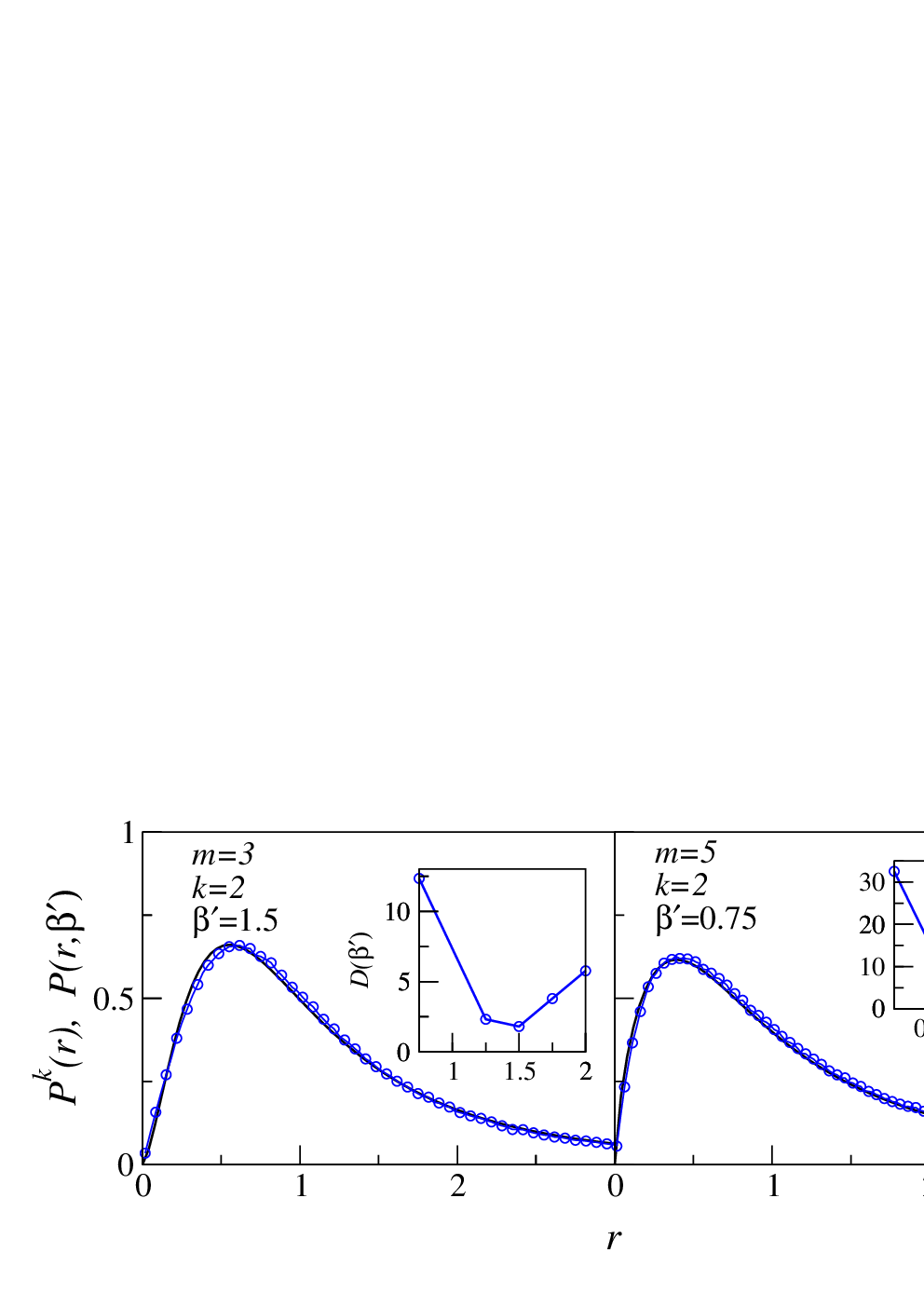
In this section, we consider the superposition of number of COEs and study its non overlapping -th order spacing ratio distribution . For COE, is taken and is used in modeling Hamiltonians which possess time-reversal symmetry and no half-integer spin Mehta 2004. This is then related with the NN spacing ratio distribution for . For given and we tabulate the value of for which both these distributions are very close to each other numerically. These values are given in Table 2 for to and various values of . It can be seen that except few all values of are whole number (this is the case for the superposition in CUEs and CSEs, which will be discussed in subsequent parts of the paper). These results are plotted in Figs. 1, 2, 3, 4 and 5. The insets shows the function, the minimum of which gives the best fit to the numerical data . Its detailed definition and other numerical methods with which we find will be discussed in Section VII. We have also plotted a representative data for noninteger in Sec.V (see Fig.14) where we have studied the superposition of CUEs.
The is an interesting case for which we have obtained scaling relations for even and odd values of and as given below:
| (6) |
and
| (7) |
For even the scaling relation reduces to Eq. (3) for by suitable change of variables as where . This is a known result on the connection between CUE and superposition of two COEs Dyson 1962a; Gunson 1962. For odd changing the variable as then Eq. 7 reduces to a simpler form as for . It can be compared with Eq. (3) and can be seen that it does not reduces to Eq. (3) for any . Thus, using the scaling relation in Eq. (7), no statement can be made at the level of jpdf of circular -ensemble.
Based on the results in Table 2, we have given two conjectures on the lines of Eq.(4) (see Ref.Tekur and Santhanam 2020) at the level of spectral fluctuations. The first conjecture is as follows:
| (8) |
and , while the second one is as follows:
| (9) |
and . Our conjectures hold true for asymptotic value of . These conjectures have appeared in our arXiv preprint Bhosale 2019.
| 1 | 0 | 0 | 0 | 0 | 0 | 0 |
|---|---|---|---|---|---|---|
| 2 | 2 | 1.25 | 1 | 1 | 0.75 | 0.75 |
| 3 | 4 | 3 | 2.5 | 2 | 2 | 2 |
| 4 | 7 | 5 | 4 | 3.5 | 3 | 3 |
| 5 | 10 | 7.5 | 6 | 5 | 5 | 4 |
| 6 | 14 | 10 | 8 | 7 | 6 | 6 |
| 7 | 18 | 13 | 11 | 9 | 8 | 7 |
| 8 | 23 | 17 | 13 | 12 | 10 | 9 |
| 9 | 28 | 20 | 16 | 14 | 12 | 11 |
| 10 | 34 | 24 | 20 | 17 | 15 | 13 |
| 11 | 40 | 29 | 23 | 20 | 17 | 16 |
| 12 | 47 | 33 | 27 | 23 | 20 | 18 |
| 13 | 54 | 38 | 31 | 26 | 23 | 21 |
| 14 | 43 | 35 | 30 | 26 | 23 | |
| 15 | 49 | 39 | 33 | 29 | 26 | |
| 16 | 44 | 32 | 29 | |||
| 17 | 32 | |||||
| 18 | 35 | |||||
| 19 | 39 | |||||
| 20 | 42 |


IV Testing RMT results to physical systems
In this section, we test our COE results on the physical model of the quantum kicked top (QKT), experimentally measured data of nuclear resonances and a spin Hamiltonian. Using these systems it will be shown that our results hold true for case. First, we consider the model of QKT. This is a fundamental and important time-dependent model for the chaotic Hamiltonian system. This model was introduced in Haake et al. 1987 and has been the topic of theoretical and experimental research since then Haake et al. 1987; Zakrzewski and Kuś 1991; Alicki et al. 1996; Weinstein et al. 2002; Demkowicz-Dobrzański and Kuś 2004; Chaudhury et al. 2009; Lombardi and Matzkin 2011; Puchała et al. 2016; Neill et al. 2016; Bhosale and Santhanam 2017; Ruebeck et al. 2017; Bhosale and Santhanam 2018; Krithika et al. 2019; Meier et al. 2019; Muñoz Arias et al. 2020; Xu et al. 2020; Kumar 2020. It has been realized in various experiments, namely, the hyperfine states of cold atoms Chaudhury et al. 2009, three coupled superconducting qubits Neill et al. 2016 and in a two-qubit NMR system Krithika et al. 2019. This is also an important model from the perspective of random matrix theory and quantum information. This model shows regular to chaotic behavior as a function of chaoticity parameter. Effects of the underlying phase space on various measures quantum correlations are studied Miller and Sarkar 1999; Neill et al. 2016; Bhosale and Santhanam 2017; Ruebeck et al. 2017. For classical limit being fully chaotic, the NN fluctuations of symmetry reduced spectra of the QKT corresponds to that of COE ensemble Haake et al. 1987; Bohigas et al. 1984.
QKT is characterized by an angular momentum vector and its components obey the standard algebra of angular momentum. The unitary time evolution operator for QKT is given as follows:
| (10) |
It represents free precession of the top around axis with angular frequency while the second term is periodic kicks applied to the top. Here, is called as the kick strength or chaos parameter. For the top is integrable and for it becomes increasingly chaotic. For given the Hilbert space dimension is equal to .
As discussed in Ref.Haake et al. 1987, for , the case relevant for us, there are two symmetries present in QKT, since commutes with the rotation operator having two eigenvalues. Thus, the matrix representation of in the basis of is block diagonal consisting of two blocks and their dimensions are and . The large case is relevant of us as these dimensions are very close to each other. For the fully chaotic case, the eigenvalue fluctuations of in each such block is found to follow COE statistics Haake et al. 1987. Taking these eigenvalues together and studying their higher-order spacings ratio is an ideal case for our study. We can compare them with our COE results of .
For our study and twenty realizations for large and different values of is taken. Thus, the dimension of the matrix is . The dimension of two blocks when is written in the eigenbasis of is and respectively. Thus, we can test our RMT results of case of COE. The results are plotted in Figs. 6 and 7 for to . It can be seen here that the results agree very well with the RMT results, case of COE in Table 2, thus implying that there are two symmetries in the QKT which we were already known apriori Haake et al. 1987. The RMT results hold true for such a large value of due to the uniform density in both, the COE ensemble and the QKT (as discussed in the Sec.II).
Now, we go on to test our results to experimentally measured nuclear resonances of Tantalum (Ta181) Hacken et al. 1978; Brody et al. 1981. It is known that it belongs to the GOE and there are two symmetries present in it Hacken et al. 1978; Brody et al. 1981. We have such resonances and the results are plotted in Fig.(8). The value of is chosen such that is best fit to the data. The results are compared with case of COE in Table 2. It can be seen that the results hold true only for and . From onwards we observe deviations from our RMT results. This is due to the nonuniversal effects in the DOS (not shown here) and the small sample size. With this example, we have tested our COE result on a GOE system with small sample size and found the number of symmetries in it successfully.
Now, a Hamiltonian corresponding to spin-1/2 chain Gubin and Santos 2012; Hsu and Angle‘s d’Auriac 1993 is considered as follows:
| (11) |
where is total number of sites, the NN coupling strengths in three directions are denoted by and (couplings in and directions are same). Similarly, and are the next-NN coupling strengths. For this Hamiltonian is integrable Tekur and Santhanam 2020. Whereas it is chaotic for and follows GOE statistics Gubin and Santos 2012. There are various symmetries in this model Santos 2009; Kudo and Deguchi 2005. The first one is due to conservation of total spin in the direction denoted as . For our work we are restricting to the case (even ) and (odd ) such that the block-matrix is of maximum possible dimension. The Hamiltonian commutes with the parity operator with eigenvalues leading to two invariant subspaces in a given block. Results for this case are plotted in Fig.9 for odd value of . It can be seen that our RMT results for case from Table2 holds true for , and . For even , the Hamiltonian also commutes with the operator corresponding to rotation symmetry with eigenvalues . Thus, in this case there will be totally four invariant subspaces in a given block. The results for this case are plotted in Figs.10 and 11. In this case our results hold from to with the corresponding RMT results for from Table2. Thus, our and the COE results agree with spin Hamiltonian having GOE statistics when there are two and four symmetries are present in it respectively. In the later case the block-matrix dimension is whereas in the previous case it is . In this case also the deviations are due to the nonuniversal effects in DOS which is Gaussian in nature (not shown here). But the results seems to improve due to the increased matrix dimension.


V Superposition and higher-order spacing ratios in CUE
In this section, we study higher-order spacings ratio in the superposition of CUEs on the lines of Section III where superposition of COEs is studied. The CUE is used in modelling Hamiltonians which lack time-reversal symmetry Mehta 2004. The results are tabulated in Table 3 for to and various values of . In this case also except few all values of are the whole number. The results are plotted in Figs.12, 13 and 14. The Fig.14 shows noninteger values of which is found by best fit.
| 1 | 0 | 0 | 0 | 0 |
|---|---|---|---|---|
| 2 | 3 | 1.5 | 1 | 0.75 |
| 3 | 6 | 4 | 3 | 2 |
| 4 | 11 | 7 | 6 | 4 |
| 5 | 15 | 11 | 8 | 7 |
| 6 | 22 | 15 | 11 | 10 |
| 7 | 28 | 20 | 15 | 13 |
| 8 | 36 | 25 | 20 | 16 |
| 9 | 43 | 31 | 24 | 20 |
| 10 | 55 | 37 | 29 | 24 |
| 11 | 64 | 44 | 34 | 28 |
| 12 | 75 | 51 | 40 | 33 |
| 13 | 59 | |||
| 14 | 67 | |||
| 15 | 76 | |||
| 16 | 85 |
In the case of superposing of CUEs is an interesting case for which we have obtained a scaling relation for even and odd values of and as given below:
| (12) |
and
| (13) |
By suitable change of variables as the Eq. 12 reduces to where . While using the Eq. 13 reduces to where . Comparing these series with Eq. (3) one can see that it does not reduce to Eq. (3) for any . Thus, using the scaling relations in Eqs. (12) and (13) no statement can be made at the level of jpdf of circular -ensemble.


VI Superposition and higher-order spacing ratios in CSE
In this section, we study higher-order spacings ratio in the superposition of CSEs on the lines of Section III. The CSE is used in modeling Hamiltonians with time-reversal symmetry and half-integer spin interaction Mehta 2004; Zyczkowski 1995. The results are tabulated in Table 4 for to and various values of . The results are plotted in Fig. 15 and 16. In this case also except few all values of are whole number.
Based on results in Table 4, we have given two conjectures at the level of spectral fluctuations. The first conjecture is as follows:
| (14) |
and , while the second one is as follows:
| (15) |
and . Our conjectures hold true for asymptotic value of .
Although we are able to find scaling relations only for few cases, but for given one can compare the sequence of as a function of with that of , within and across the Tables 2, 3 and 4. It can be seen that these sequences are unique for given and the type of ensemble considered. One can also see that this is an increasing sequence on the lines of earlier result in Eq.3 from Refs.Tekur et al. 2018c; Bhosale et al. 2018. With this observation, we would like to conjecture that for a given number of symmetries and the Dyson index of the circular ensemble or a quantum chaotic system, the sequence of is an increasing function of and completely characterize the ensemble or the system uniquely.
Similarly, for given one can compare the sequence of as a function of with that of , within and across the Tables 2, 3 and 4. Also, the sequences are unique for given and decreasing. Thus, with this observation, we would like to conjecture that for given and the Dyson index , the sequence of is decreasing as a function of and is unique. This can be interpreted physically as follows: The level repulsion present in the eigenvalues characterized by for given and is reduced as is increased and is reflected in the reduction of the new value of . The implication of this conjecture is that for given , and we will see . It can be seen easily that one conjecture does not imply the second one.
Proving our results mathematically is challenging but we give an intuitive argument for the last conjecture. We know that NN as well as the -th eigenvalues in circular or Gaussian spectra repel each other Forrester 2010. It has also been established mathematically (analytical and numerical) that when two same dimensional COE/GOE spectra are superposed the NN don’t repel each other (level clustering) in the limit of matrix dimensions tending to infinity, which results in their spacings distribution to be Poissonian Mehta 2004; Guhr et al. 1998; Tkocz et al. 2012; Smaczyński et al. 2013; Tkocz et al. 2013. In other words, before superposition, the level repulsion present (characterized by ) has now vanished after superposition (characterized by ). And this is what is also observed in our last conjecture i.e. for given and the value of (characterizing the repulsion between the -th eigenvalues) reduces as is increased. In most of the cases we studied here, although not guaranteed, these reductions are integer number. The special case of our conjecture where , and is shown to have NN spacing distribution as Poissonian in Ref.Tkocz et al. 2012.


| 1 | 0 | 0 | 0 | 0 | 0 |
|---|---|---|---|---|---|
| 2 | 5 | 2 | 1 | 0.75 | 0.75 |
| 3 | 7 | 7 | 4 | 2.5 | 2 |
| 4 | 18 | 9 | 8 | 6 | 4 |
| 5 | 21 | 14 | 11 | 10 | 8 |
| 6 | 36 | 23 | 14 | 13 | 12 |
| 7 | 39 | 27 | 21 | 16 | 15 |
| 8 | 60 | 35 | 28 | 20 | 18 |
| 9 | 63 | 47 | 33 | 27 | 21 |
| 10 | 88 | 53 | 38 | 35 | 27 |
| 11 | 92 | 63 | 48 | 40 | 34 |
| 12 | 122 | 79 | 59 | 44 | 40 |
VII Numerical methods
Now, various numerical pieces of evidence supporting our results are presented. These best fits are checked with the numerical data quantitatively.
As a numerical check for our claims, analysis using Eq. (3) for is carried, where no fitting parameter is involved. For this, the difference between the cumulative distributions is numerically found and defined as follows:
| (16) |
where and denotes cumulative distribution functions corresponding to the observed histogram and the numerical fit or the postulated function respectively. This definition has been used in earlier works Tekur and Santhanam 2020; Bhosale et al. 2018; Tekur et al. 2018c in similar kind of analysis. It can be seen that, can take any positive value (upper bound) depending on the range of in the summation, but is minimum only for that value of for which is best fit for the observed histogram. The values of for given are same as that in Figs. 1, 2, 3, 4, 5, 6, 7, 8, 9, 10, 11, 12, 13, 15 and 16. The results of are shown in the insets of these figures. It can be seen that the minima of in each case coincides remarkably with that of corresponding from the main figures.
After finding the best fit for the observed data using , we go on to check how close the two probability distributions and their respective cumulative fuctions are. Firstly, the overlap () between the probability plots in Figs. 1, 2, 3, 4, 5, 6, 7, 8, 9, 10, 11, 12, 13, 15 and 16 is calculated using the following definition:
| (17) |
Secondly, the cumulative distribution functions corresponding to observed data and is studied. The maximum absolute difference () between these cumulative distributions is calculated using the following definition:
| (18) |
By definition and larger (smaller) value of () will indicate that the numerically observed distribution is close to that of the postulated one. Unlike , these values will only improve as the range of is increased. The values are shown in Tables 5, 6, 7, 8, 9, 10 and 11. The Tables 5, 6, 7 and 8 gives strong evidences for our results in Tables 2, 3 and 4 corresponding to the superposition of COE, CUE and CSE respectively. In Tables 9, 10 and 11 results are shown for the physical system of QKT, measured nuclear resonances and the spin Hamiltonian as plotted in Figs.6, 7, 8, 9, 10 and 11. It can be seen that in all the cases the values of and shown in these tables gives strong evidences for our results in these figures. The effect of small sample size in the case of nuclear resonances can be seen in the Table 10.
| 3 | 3 | 2 | |||||
| 5 | 4 | 4 | |||||
| 7 | 6 | 5 | |||||
| 9 | 7 | 6 | |||||
| 11 | 8 | 7 | |||||
| 13 | 9 | 8 | |||||
| 10 | 9 | ||||||
| 11 | 11 | ||||||
| 12 | 13 | ||||||
| 13 | 15 |
| 2 | 3 | 3 | |||||
| 3 | 4 | 4 | |||||
| 6 | 5 | 5 | |||||
| 7 | 6 | 6 | |||||
| 8 | 7 | 7 | |||||
| 9 | 8 | 8 | |||||
| 10 | 9 | 9 | |||||
| 11 | 10 | 10 | |||||
| 12 | 12 | 15 | |||||
| 13 | 16 | 20 |
| 3 | 9 | |||
| 4 | 10 | |||
| 5 | 11 | |||
| 6 | 12 | |||
| 7 | 13 | |||
| 8 | 14 |
| 2 | 4 | 3 | |||||
| 3 | 5 | 4 | |||||
| 4 | 6 | 5 | |||||
| 5 | 7 | 6 | |||||
| 6 | 8 | 7 | |||||
| 7 | 9 | 8 | |||||
| 8 | 10 | 9 | |||||
| 9 | 11 | 10 | |||||
| 10 | 12 | 11 | |||||
| 11 | 12 | ||||||
| 12 |
| 2 | 2 | 8 | 23 | |||
| 3 | 4 | 9 | 28 | |||
| 4 | 7 | 10 | 34 | |||
| 5 | 10 | 11 | 40 | |||
| 6 | 14 | 12 | 47 | |||
| 7 | 18 | 13 | 54 |
| 2 | 2 | 4 | 6 | |||
| 3 | 4 | 5 | 8 |
| 2 | 2 | 2 | 1 | |||
| 3 | 4 | 3 | 2.5 | |||
| 4 | 7 | 4 | 4 | |||
| 5 | 11 | 5 | 6 | |||
| 6 | 12 | 6 | 8 | |||
| 7 | 16 | 7 | 10 | |||
| 8 | 12 | |||||
| 9 | 16 | |||||
| 10 | 17 |
VIII SUMMARY AND CONCLUSIONS
This paper has studied the long-range correlations in the superposed spectra of COE, CUE and CSE using higher-order spacing ratios. We have given a table for the modified Dyson indices () corresponding to the distribution of -th order spacing ratio when number of matrices each from COEs, CUEs and CSEs are superposed. For the case when two COEs are superposed two scaling relations relating and are found for even and odd values of respectively. The relation corresponding to even is related to the earlier result on the connection between CUE and superposition of two COEs at the level of jpdf Dyson 1962a; Gunson 1962. Conjectures on the lines of Ref.Tekur and Santhanam 2020 are given. For the case of COE, it is conjectured that for given , the distribution of the -th order spacing ratio is related to such that the relation for and for holds true. Similarly, for the case of CSE, the relation for and for holds true.
We have tested our results on three different physical systems. The first one is the QKT in the quantum chaotic limit belonging to COE. The other two are the measured nuclear resonances and a spin Hamiltonian both corresponding to the GOE. These systems are known to have symmetries. For the case of QKT, we have tested our RMT results of case up to and found very good agreement. This agrees with the earlier analytical result from the Ref.Haake et al. 1987, where it is shown that its Hamiltonian has two symmetries. Whereas in the case of nuclear resonances we could find agreement only up to due to nonuniform density as well as small sample size. But the results of and were enough to conclude the presence of two symmetries using the uniqueness of our tabulated COE results. The third system we considered is the quantum chaotic spin Hamiltonian. Depending on the values of the parameter a given spin sector can have two or four symmetries. In both the cases we tested our COE results of and . In this case, also we observed effects of nonuniform density but at large values of compared to the previous case due to the large matrix dimension. These results imply that our RMT results hold very well to quantum chaotic physical systems modeled by circular ensembles. For others, we may see the deviations for higher values of depending on the system and its matrix dimension or the sample size. Despite this we could successfully find the symmetries of systems modeled by Gaussian ensembles. Looking at our results and the Refs.Mehta 2004; Forrester 2010; Tekur and Santhanam 2020; Tekur et al. 2018a; Porter 1963; Kahn and Porter 1963 specially the Ref.Tekur et al. 2018a our results can be claimed to be true for Gaussian ensembles in the limit of large matrix dimensions. Thus, our results can be used to find the symmetries in unknown physical systems.
For the case of superposition of CUEs two scaling relations relating and are found for even and odd values of . These scaling relations along with other results are confirmed numerically using large matrix dimensions. We have used various numerical tests for the verification of our results. We conjectured that for given (), the sequence of as a function of () is increasing (decreasing) and is unique to a given circular -ensemble. As a corollary, finding symmetries as well as whether a given quantum chaotic system is time-reversal invariant (with or without the spin degree of freedom) or not can be found unambiguously. The Gaussian ensembles have been implemented in various experimental systems Alt et al. 1997; Dembowski et al. 2000; Schäfer et al. 2002; Dietz et al. 2014; Rehemanjiang et al. 2016. Thus, our circular ensemble results can be tested using these experiments by taking experimental systems with suitable geometrical symmetry corresponding to given .
This work has given rise to new future directions as well. We would like to test our results as an additional and stringent test for finding symmetries in various other quantum complex systems Tekur and Santhanam 2020; Giraud et al. 2020; Srdinšek et al. 2021. Various quantum chaotic systems with and without time-reversal invariance and having additional symmetries can be tested. Our study can be extended to the case when matrices of unequal dimensions are superposed which will be relevant to understand symmetries in various other spin systems Binder and Young 1986; Amico et al. 2008; Tekur and Santhanam 2020; Giraud et al. 2020. Our study can be extended to other relevant ensembles from RMT, for example the ensembles with chiral symmetry Fyodorov and Strahov 2002; Damgaard 2011; Kaymak et al. 2014; Beenakker 2015; Akemann 2017; Mondal and Shukla 2020; Rehemanjiang et al. 2020 and Wishart ensemble Wishart 1928; Majumdar and Vergassola 2009; Akemann et al. 2011; Fridman et al. 2012; Bhosale et al. 2018.
IX Acknowledgments
Authors are grateful to M. S. Santhanam, Harshini Tekur and Ravi Prakash for useful comments and discussions at various stages of this paper. UTB thanks Rukmani Bai and Hrushikesh Sable for helping in the numerical data. The results presented in the paper are based on the computations using Mathematica 9 in Vikram-100, the 100TFLOP HPC Cluster at Physical Research Laboratory, Ahmedabad, India.
References
- Weidenmüller and Mitchell (2009) H. Weidenmüller and G. Mitchell, Reviews of Modern Physics 81, 539 (2009).
- Mitchell et al. (2010) G. E. Mitchell, A. Richter, and H. A. Weidenmüller, Reviews of Modern Physics 82, 2845 (2010).
- Haake (2010) F. Haake, Quantum Signatures of Chaos (Springer, 3rd Edition, Berlin, 2010).
- Akemann et al. (2011) G. Akemann, J. Baik, and P. Di Francesco, The Oxford handbook of random matrix theory (Oxford University Press, 2011).
- Stöckmann (1999) H.-J. Stöckmann, Quantum Chaos: An Introduction (University Press, Cambridge, 1999).
- Porter (1965) C. E. Porter, Statistical Theories of Spectra: Fluctuations (Academic Press, New York, 1965).
- Forrester (2010) P. J. Forrester, Log-Gases and Random Matrices (Princeton University Press, Princeton and Oxford, 2010).
- Mehta (2004) M. L. Mehta, Random Matrices (Elsevier Academic Press, 3rd Edition, London, 2004).
- Guhr et al. (1998) T. Guhr, A. Müeller-Groeling, and H. A. Weidenmüeller, Phys. Rep. 299, 189 (1998).
- Hutchinson et al. (2015) J. Hutchinson, J. Keating, and F. Mezzadri, Physical Review E 92, 032106 (2015).
- Wells (2014) H. J. Wells, arXiv preprint arXiv:1410.1666 (2014).
- Rao (2020a) W.-J. Rao, Physical Review B 102, 054202 (2020a).
- Rao (2021a) W.-J. Rao, Journal of Physics A: Mathematical and Theoretical 54, 105001 (2021a).
- Rao (2021b) W.-J. Rao, arXiv preprint arXiv:2105.04468 (2021b).
- Gómez et al. (2011) J. Gómez, K. Kar, V. Kota, R. A. Molina, A. Relaño, and J. Retamosa, Physics Reports 499, 103 (2011).
- Bohigas et al. (1984) O. Bohigas, M. J. Giannoni, and C. Schmit, Phys. Rev. Lett. 52, 1 (1984).
- Hurt (2013) N. E. Hurt, Quantum chaos and mesoscopic systems: mathematical methods in the quantum signatures of chaos, vol. 397 (Springer Science & Business Media, 2013).
- Oganesyan and Huse (2007a) V. Oganesyan and D. A. Huse, Phys. Rev. B 75, 155111 (2007a).
- Haake et al. (1987) F. Haake, M. Kus, and R. Scharf, Z. Phys. B 65, 381 (1987).
- Reichl (2004) L. E. Reichl, The Transition to Chaos, 2nd edition (Springer-Verlag, New York, 2004).
- Tekur and Santhanam (2020) S. H. Tekur and M. S. Santhanam, Phys. Rev. Research 2, 032063 (2020).
- Dyson (1962a) F. J. Dyson, J. Math. Phys. 3, 166 (1962a).
- Gunson (1962) J. Gunson, Journal of Mathematical Physics 3, 752 (1962).
- Anderson et al. (2010) G. W. Anderson, A. Guionnet, and O. Zeitouni, An introduction to random matrices, vol. 118 (Cambridge university press, 2010).
- Giraud et al. (2020) O. Giraud, N. Macé, E. Vernier, and F. Alet, arXiv preprint arXiv:2008.11173 (2020).
- Santos and Rigol (2010a) L. F. Santos and M. Rigol, Phys. Rev. E 82, 031130 (2010a).
- Gubin and Santos (2012) A. Gubin and L. F. Santos, Am. J. Phys. 80, 246 (2012).
- Brading and Castellani (2003) K. Brading and E. Castellani, Symmetries in physics: philosophical reflections (Cambridge University Press, 2003).
- Corry (2016) S. Corry, Symmetry and Quantum Mechanics (Chapman and Hall/CRC, 2016).
- Gross (1996) D. J. Gross, Proceedings of the National Academy of Sciences 93, 14256 (1996).
- Rosen (2008) J. Rosen, Symmetry rules: How science and nature are founded on symmetry (Springer Science & Business Media, 2008).
- Tapp (2011) K. Tapp, Symmetry: a mathematical exploration (Springer Science & Business Media, 2011).
- Longo and Montévil (2013) G. Longo and M. Montévil, Perspectives on organisms: Biological time, symmetries and singularities (Springer Science & Business Media, 2013).
- Sardanashvily (2016) G. Sardanashvily, Noether’s Theorems (Springer, 2016).
- Kosmann-Schwarzbach (2011) Y. Kosmann-Schwarzbach, in The Noether Theorems (Springer, 2011), pp. 55–64.
- Cotler et al. (2017) J. S. Cotler, G. Gur-Ari, M. Hanada, J. Polchinski, P. Saad, S. H. Shenker, D. Stanford, A. Streicher, and M. Tezuka, Journal of High Energy Physics 2017, 118 (2017).
- Tekur et al. (2018a) S. H. Tekur, U. T. Bhosale, and M. Santhanam, Phys. Rev. B 98, 104305 (2018a).
- Porter (1963) C. E. Porter, Nuclear Physics 40, 167 (1963).
- Kahn and Porter (1963) P. B. Kahn and C. E. Porter, Nuclear Physics 48, 385 (1963).
- Dumitriu and Edelman (2002) I. Dumitriu and A. Edelman, Journal of Mathematical Physics 43, 5830 (2002).
- Buijsman et al. (2019) W. Buijsman, V. Cheianov, and V. Gritsev, Phys. Rev. Lett. 122, 180601 (2019).
- Sierant and Zakrzewski (2019) P. Sierant and J. Zakrzewski, Phys. Rev. B 99, 104205 (2019).
- Berry (1985) M. V. Berry, Proc. R. Soc. A 400, 229 (1985).
- Sieber and Richter (2001) M. Sieber and K. Richter, Physica Scripta 2001, 128 (2001).
- Müller et al. (2009) S. Müller, S. Heusler, A. Altland, P. Braun, and F. Haake, New Journal of Physics 11, 103025 (2009).
- Tkocz et al. (2012) T. Tkocz, M. Smaczyński, M. Kuś, O. Zeitouni, and K. Życzkowski, Random Matrices: Theor. Appl. 1, 1250009 (2012).
- Smaczyński et al. (2013) M. Smaczyński, T. Tkocz, M. Kuś, and K. Życzkowski, Phys. Rev. E 88, 052902 (2013).
- Tkocz et al. (2013) T. Tkocz et al., Electronic communications in probability 18 (2013).
- Berry and Tabor (1977) M. V. Berry and M. Tabor, Proc. R. Soc. Lond. A 356, 375 (1977).
- Dyson (1962b) F. J. Dyson, J. Math. Phys. 3, 140 (1962b).
- Mezzadri (2007) F. Mezzadri, Notices of the AMS 54, 592 (2007).
- Killip and Nenciu (2004) R. Killip and I. Nenciu, International Mathematics Research Notices 2004, 2665 (2004).
- Mehta and Dyson (1963) M. L. Mehta and F. J. Dyson, J. Math. Phys. 4, 713 (1963).
- Bruus and Angl‘es d’Auriac (1997) H. Bruus and J.-C. Angl‘es d’Auriac, Phys. Rev. B 55, 9142 (1997).
- Gómez et al. (2002) J. M. G. Gómez, R. A. Molina, A. Relaño, and J. Retamosa, Phys. Rev. E 66, 036209 (2002).
- Oganesyan and Huse (2007b) V. Oganesyan and D. A. Huse, Phys. Rev. B 75, 155111 (2007b).
- Atas et al. (2013a) Y. Y. Atas, E. Bogomolny, O. Giraud, and G. Roux, Phys. Rev. Lett. 110, 084101 (2013a).
- Atas et al. (2013b) Y. Atas, E. Bogomolny, O. Giraud, P. Vivo, and E. Vivo, Journal of Physics A: Mathematical and Theoretical 46, 355204 (2013b).
- Oganesyan et al. (2009) V. Oganesyan, A. Pal, and D. A. Huse, Phys. Rev. B 80, 115104 (2009).
- Pal and Huse (2010) A. Pal and D. A. Huse, Phys. Rev. B 82, 174411 (2010).
- Iyer et al. (2013) S. Iyer, V. Oganesyan, G. Refael, and D. A. Huse, Phys. Rev. B 87, 134202 (2013).
- Cuevas et al. (2012) E. Cuevas, M. Feigel’Man, L. Ioffe, and M. Mezard, Nature communications 3, 1128 (2012).
- Biroli et al. (2012) G. Biroli, A. Ribeiro-Teixeira, and M. Tarzia, arXiv preprint arXiv:1211.7334 (2012).
- Chen et al. (2018) C. Chen, F. Burnell, and A. Chandran, Phys. Rev. Lett. 121, 085701 (2018).
- Santos and Rigol (2010b) L. F. Santos and M. Rigol, Phys. Rev. E 81, 036206 (2010b).
- Kollath et al. (2010) C. Kollath, G. Roux, G. Biroli, and A. M. Läuchli, Journal of Statistical Mechanics: Theory and Experiment 2010, P08011 (2010).
- Rigol and Santos (2010) M. Rigol and L. F. Santos, Phys. Rev. A 82, 011604 (2010).
- Collura et al. (2012) M. Collura, H. Aufderheide, G. Roux, and D. Karevski, Phys. Rev. A 86, 013615 (2012).
- Tarquini et al. (2016) E. Tarquini, G. Biroli, and M. Tarzia, Phys. Rev. Lett. 116, 010601 (2016).
- Corps and Relaño (2020) A. L. Corps and A. Relaño, Phys. Rev. E 101, 022222 (2020).
- Sun and Ye (2020) F. Sun and J. Ye, Phys. Rev. Lett. 124, 244101 (2020).
- Sun et al. (2020) F. Sun, Y. Yi-Xiang, J. Ye, and W.-M. Liu, Phys. Rev. D 101, 026009 (2020).
- Nosaka and Numasawa (2020) T. Nosaka and T. Numasawa, Journal of High Energy Physics 2020, 1 (2020).
- Srdinsek et al. (2020) M. Srdinsek, T. Prosen, and S. Sotiriadis, arXiv preprint arXiv:2012.08505 (2020).
- Chavda et al. (2014) N. Chavda, H. Deota, and V. Kota, Physics Letters A 378, 3012 (2014).
- Kota and Chavda (2018) V. Kota and N. Chavda, International Journal of Modern Physics E 27, 1830001 (2018).
- Tekur et al. (2018b) S. H. Tekur, S. Kumar, and M. S. Santhanam, Phys. Rev. E 97, 062212 (2018b).
- Sá et al. (2020) L. Sá, P. Ribeiro, and T. Prosen, Phys. Rev. X 10, 021019 (2020).
- Tekur et al. (2018c) S. H. Tekur, U. T. Bhosale, and M. S. Santhanam, Phys. Rev. B 98, 104305 (2018c).
- Bhosale et al. (2018) U. T. Bhosale, S. H. Tekur, and M. S. Santhanam, Phys. Rev. E 98, 052133 (2018).
- Rao et al. (2020) P. Rao, M. Vyas, and N. D. Chavda, The European Physical Journal Special Topics 229, 2603 (2020).
- Brody et al. (1981) T. A. Brody, J. Flores, J. B. French, P. A. Mello, A. Pandey, and S. S. M. Wong, Rev. Mod. Phys. 53, 385 (1981).
- Abul-Magd and Simbel (1999) A. Y. Abul-Magd and M. H. Simbel, Phys. Rev. E 60, 5371 (1999).
- Katz and Sarnak (1999) N. M. Katz and P. Sarnak, Bull. Am. Math. 31, 1 (1999).
- Keating and Snaith (2003) J. P. Keating and N. C. Snaith, J. Phys. A: Math. Gen. 36, 2859 (2003).
- Rao (2020b) W.-J. Rao, Phys. Rev. B 102, 054202 (2020b).
- Rao and Chen (2020) W.-J. Rao and M. Chen, arXiv preprint arXiv:2006.07774 (2020).
- Forrester and Rains (2004) P. J. Forrester and E. M. Rains, Probability theory and related fields 130, 518 (2004).
- Forrester (2009) P. J. Forrester, Communications in mathematical physics 285, 653 (2009).
- Bhosale (2019) U. T. Bhosale, arXiv preprint arXiv:1905.02585 (2019).
- Zakrzewski and Kuś (1991) J. Zakrzewski and M. Kuś, Phys. Rev. Lett. 67, 2749 (1991).
- Alicki et al. (1996) R. Alicki, D. Makowiec, and W. Miklaszewski, Phys. Rev. Lett. 77, 838 (1996).
- Weinstein et al. (2002) Y. S. Weinstein, S. Lloyd, and C. Tsallis, Phys. Rev. Lett. 89, 214101 (2002).
- Demkowicz-Dobrzański and Kuś (2004) R. Demkowicz-Dobrzański and M. Kuś, Phys. Rev. E 70, 066216 (2004).
- Chaudhury et al. (2009) S. Chaudhury, A. Smith, B. E. Anderson, S. Ghose, and P. S. Jessen, Nature 461, 768 (2009).
- Lombardi and Matzkin (2011) M. Lombardi and A. Matzkin, Phys. Rev. E 83, 016207 (2011).
- Puchała et al. (2016) Z. Puchała, L. Pawela, and K. Życzkowski, Phys. Rev. A 93, 062112 (2016).
- Neill et al. (2016) C. Neill, P. Roushan, M. Fang, Y. Chen, M. Kolodrubetz, Z. Chen, A. Megrant, R. Barends, B. Campbell, B. Chiaro, et al., Nature Physics (2016).
- Bhosale and Santhanam (2017) U. T. Bhosale and M. S. Santhanam, Phys. Rev. E 95, 012216 (2017).
- Ruebeck et al. (2017) J. B. Ruebeck, J. Lin, and A. K. Pattanayak, Phys. Rev. E 95, 062222 (2017).
- Bhosale and Santhanam (2018) U. T. Bhosale and M. S. Santhanam, Phys. Rev. E 98, 052228 (2018).
- Krithika et al. (2019) V. R. Krithika, V. S. Anjusha, U. T. Bhosale, and T. S. Mahesh, Phys. Rev. E 99, 032219 (2019).
- Meier et al. (2019) E. J. Meier, J. Ang’ong’a, F. A. An, and B. Gadway, Phys. Rev. A 100, 013623 (2019).
- Muñoz Arias et al. (2020) M. H. Muñoz Arias, P. M. Poggi, P. S. Jessen, and I. H. Deutsch, Phys. Rev. Lett. 124, 110503 (2020).
- Xu et al. (2020) T. Xu, T. Scaffidi, and X. Cao, Phys. Rev. Lett. 124, 140602 (2020).
- Kumar (2020) S. Kumar, Phys. Rev. A 102, 012405 (2020).
- Miller and Sarkar (1999) P. A. Miller and S. Sarkar, Phys. Rev. E 60, 1542–1550 (1999).
- Hacken et al. (1978) G. Hacken, R. Werbin, and J. Rainwater, Phys. Rev. C 17, 43 (1978).
- Hsu and Angle‘s d’Auriac (1993) T. C. Hsu and J. C. Angle‘s d’Auriac, Phys. Rev. B 47, 14291 (1993).
- Santos (2009) L. F. Santos, Journal of mathematical physics 50, 095211 (2009).
- Kudo and Deguchi (2005) K. Kudo and T. Deguchi, Journal of the Physical Society of Japan 74, 1992 (2005).
- Zyczkowski (1995) K. Zyczkowski, in Chaos-The Interplay Between Stochastic and Deterministic Behaviour (Springer, 1995), pp. 565–571.
- Alt et al. (1997) H. Alt, H.-D. Gräf, T. Guhr, H. L. Harney, R. Hofferbert, H. Rehfeld, A. Richter, and P. Schardt, Phys. Rev. E 55, 6674 (1997).
- Dembowski et al. (2000) C. Dembowski, H.-D. Gräf, A. Heine, H. Rehfeld, A. Richter, and C. Schmit, Phys. Rev. E 62, R4516 (2000).
- Schäfer et al. (2002) R. Schäfer, M. Barth, F. Leyvraz, M. Müller, T. H. Seligman, and H.-J. Stöckmann, Phys. Rev. E 66, 016202 (2002).
- Dietz et al. (2014) B. Dietz, T. Guhr, B. Gutkin, M. Miski-Oglu, and A. Richter, Phys. Rev. E 90, 022903 (2014).
- Rehemanjiang et al. (2016) A. Rehemanjiang, M. Allgaier, C. H. Joyner, S. Müller, M. Sieber, U. Kuhl, and H.-J. Stöckmann, Phys. Rev. Lett. 117, 064101 (2016).
- Srdinšek et al. (2021) M. Srdinšek, T. c. v. Prosen, and S. Sotiriadis, Phys. Rev. Lett. 126, 121602 (2021).
- Binder and Young (1986) K. Binder and A. P. Young, Reviews of Modern physics 58, 801 (1986).
- Amico et al. (2008) I. Amico, R. Fazio, and A. Osterloh, Rev. Mod. Phys. 80, 517 (2008).
- Fyodorov and Strahov (2002) Y. V. Fyodorov and E. Strahov, Nuclear Physics B 647, 581 (2002).
- Damgaard (2011) P. H. Damgaard, in Journal of Physics: Conference Series (IOP Publishing, 2011), vol. 287, p. 012004.
- Kaymak et al. (2014) V. Kaymak, M. Kieburg, and T. Guhr, Journal of Physics A: Mathematical and Theoretical 47, 295201 (2014).
- Beenakker (2015) C. W. J. Beenakker, Rev. Mod. Phys. 87, 1037 (2015).
- Akemann (2017) G. Akemann, Stochastic Processes and Random Matrices: Lecture Notes of the Les Houches Summer School 104, 228 (2017).
- Mondal and Shukla (2020) T. Mondal and P. Shukla, Phys. Rev. E 102, 032131 (2020).
- Rehemanjiang et al. (2020) A. Rehemanjiang, M. Richter, U. Kuhl, and H.-J. Stöckmann, Phys. Rev. Lett. 124, 116801 (2020).
- Wishart (1928) J. Wishart, Biometrika 20A, 32 (1928).
- Majumdar and Vergassola (2009) S. N. Majumdar and M. Vergassola, Phys. Rev. Lett. 102, 060601 (2009).
- Fridman et al. (2012) M. Fridman, R. Pugatch, M. Nixon, A. A. Friesem, and N. Davidson, Phys. Rev. E 85, 020101 (2012).