Rational spectral methods for PDEs involving fractional Laplacian in unbounded domainsThanks: The work of the first author is supported by the National Natural Science Foundations of China under grant 91630312. The research of the second author is supported by Singapore MOE AcRF Tier 2 Grants: MOE2017-T2-2-014 and MOE2018-T2-1-059. The third author is supported by a Hong Kong PhD Fellowship. The last author is partially supported by the NSF of China (under grant numbers 11822111, 11688101, 91630203, 11571351, and 11731006), the science challenge project (No. TZ2018001), NCMIS, and the youth innovation promotion association (CAS).

Tao Tang¹¹ 1 Department of Mathematics, Southern University of Sciences and Technology, Shenzhen, China (tangt@sustc.edu.cn) Li-Lian Wang²² 2 Division of Mathematical Sciences, School of Physical and Mathematical Sciences, Nanyang Technological University, Singapore, 637371 (lilian@ntu.edu.sg) Huifang Yuan³³ 3 Department of Mathematics, Hong Kong Baptist University, Hong Kong, China (13480510@life.hkbu.edu.hk) Tao Zhou⁴⁴ 4 LSEC, Institute of Computational Mathematics, Academy of Mathematics and Systems Science, Chinese Academy of Sciences, Beijing, China (tzhou@lsec.cc.ac.cn)

Abstract

Many PDEs involving fractional Laplacian are naturally set in unbounded domains with underlying solutions decay very slowly, subject to certain power laws. Their numerical solutions are under-explored. This paper aims at developing accurate spectral methods using rational basis (or modified mapped Gegenbauer functions) for such models in unbounded domains. The main building block of the spectral algorithms is the explicit representations for the Fourier transform and fractional Laplacian of the rational basis, derived from some useful integral identites related to modified Bessel functions. With these at our disposal, we can construct rational spectral-Galerkin and direct collocation schemes by pre-computing the associated fractional differentiation matrices. We obtain optimal error estimates of rational spectral approximation in the fractional Sobolev spaces, and analyze the optimal convergence of the proposed Galerkin scheme. We also provide ample numerical results to show that the rational method outperforms the Hermite function approach.

keywords

Fractional Laplacian, Gegenbauer polynomials, modified rational functions, unbounded domains, Fourier transforms, spectral methods.

AMS

65N35, 65M70, 41A05, 41A25.

\slugger

mmsxxxxxxxx–x

1 Introduction

Diffusion is a ubiquitous physical process, typically modeled by partial differential equations (PDEs) with usual Laplacian operators. Although they can describe the anisotropy of diffusion, many systems in science, economics and engineering exhibit anomalous diffusion, which can be more accurately and realistically modelled by PDEs with fractional Laplacian operators [4, 5, 13]. In the past decade, tremendous research attention has been paid to the analysis and numerical studies of fractional PDEs. The finite difference method and the finite element method are two widely studied methods in this direction (see, e.g., [18, 19, 20, 9, 40, 3, 43, 36, 44, 45, 41] and references therein). Most of efforts are devoted to dealing with the nonlocal nature or singularities of the fractional operators. Another powerful approach is the spectral method, which is more suitable for the non-local feature of the fractional operators (see, e.g., [47, 11, 10, 21, 25, 34, 35, 46, 37]). However, most of these works are for fractional problems in bounded domains. In particular, we refer to Bonito et al [6] for an up-to-date review of the various numerical methods for fractional diffusion based on different formulations of the fractional Laplacian.

It is known that many physically motivated fractional diffusive problems are naturally set in unbounded domains, but their investigation is still under-explored. For usual PDEs in unbounded domains, several approaches have been widely used in practice (see, e.g., [8, 32] and the original references cited therein). The first is direct domain truncation that works well for problems with rapidly decaying solutions, but is not feasible for fractional problems as the underlying solutions usually decay slowly, subject to certain power laws at infinity. On the other hand, the naive truncation introduces nonphysical singularities at the interface where the unbounded domain is terminated. The second is to design a suitable transparent boundary condition or artificial sponge layer, but this appears highly nontrivial for the fractional Laplacian. The third is the use of orthogonal functions in unbounded domains, which has been successfully applied to many usual PDEs (see, e.g., [38, 8, 14, 27, 32, 31]). Very recently, spectral methods for fractional PDEs on the half line are proposed by [22, 25] – using the generalized Laguerre functions as bases – extending the idea of [47]. A two-domain spectral approximations by Laguerre functions is developed in [12] for tempered fractional PDEs on the whole line. Mao and Shen [28] proposed both spectral-Galerkin and collocation methods using Hermite functions for fractional PDEs in unbounded domains. However, the collocation method therein relies on an equivalent formulation in frequency space by the Fourier transforms, and performs collocation methods to the equivalent formulation that involve forward/backward Hermite transforms. Tang, Yuan and Zhou [39] developed direct Hermite collocation methods with explicit formulations for the differentiation matrices, which is therefore more robust for nonlinear problems. Lastly, spectral approximation using non-classical orthogonal functions in unbounded domains – image of classical Jacobi polynomials through a suitable mapping, has proven to be more viable for usual PDEs with solutions decaying algebraically (see, e.g., [7, 8, 16, 17, 30]), compared with approximation by Hermite/Laguerre functions. As such, the rational basis (or mapped Jacobi functions) should be more desirable for PDEs with fractional Laplacian, due to the slow decaying solution with long tails subject to certain power law. However, to the best of our knowledge, there is essentially no work available along this line. Moreover, the extension of the mapping technique to the fractional setting is far from trivial, as we elaborate on below.

In this paper, we intend to fill in this gap, and design rational spectral methods for a class of PDEs with fractional Laplacian in $\mathbb{R}^{d}$ . To fix the idea, we consider the model equation:

\begin{cases}(-\Delta)^{\alpha/2}u(x)+\rho u(x)=f(x),\quad&x\in{\mathbb{R}}^{d},\\ u(x)=0,\quad&\lvert x\rvert\to\infty,\end{cases}

(1)

for $\alpha\in(0,2),$ where the fractional Laplace operator is defined as in [23]:

(-\Delta)^{\alpha/2}u(x):=C_{d,\alpha}{\rm p.v.}\int_{\mathbb{R}^{d}}\dfrac{u(x)-u(y)}{\lvert x-y\rvert^{d+\alpha}}dy\;\;\textmd{with}\;\;C_{d,\alpha}:=\dfrac{{\alpha}2^{\alpha-1}\Gamma\Big(\dfrac{\alpha+d}{2}\Big)}{\pi^{d/2}\Gamma\Big(\dfrac{2-\alpha}{2}\Big)}.

(2)

Here, p.v. stands for the Cauchy principal value, and $C_{d,\alpha}$ is a normalization constant. Equivalently, the fractional Laplacian can be defined as a pseudo-differential operator via the Fourier transform:

(-\Delta)^{\alpha/2}u(x):={\mathscr{F}}^{-1}\big[|\xi|^{\alpha}\mathscr{F}{\left[u\right]}({\xi})\big](x).

(3)

For any expansion-based method, a critical issue is how to accurately evaluate the point-wise value of the fractional Laplacian performing upon the basis. For example, the key to the Hermite spectral method in [28] is the use of the attractive property that the Hermtie functions are the eigenfunctions of the Fourier transform, so the algorithm is largely implemented in the frequency $\xi$ -space. In contrast, some analytically perspicuous formulas of $(-\Delta)^{\alpha/2}$ on the Hermite functions were derived in [39], which led themselves to the construction of efficient collocation algorithms in the physical $x$ -space. In the spirit of [39], we search for the analytic formulas for computing the fractional Laplacian of the rational basis functions – the modified mapped Gegenbauer functions (MMGFs), orthogonal with respect to a uniform weight. Although the formulas (see Theorem 4) are not as compact as those for the Hermite functions, we can accurately compute the fractional Laplacian of the rational basis up to the degree $\thicksim 10^{3}$ by using e.g., Maple or Mathematica. Moreover, with these analytic tools at our disposal, we are able to study their asymptotic behaviors and dependence of the parameters so that the basis can be tailored to the decay rate of underlying solution. We propose and analyze a spectral-Galerkin scheme, and obtain optimal estimates (see Theorem 9). We also implement a direct collocation scheme based on the associated fractional differentiation matrices with the aid of the aforementioned explicit formulas. However, its error analysis appears very challenging and largely open. This is mostly for the reason that the fractional Laplacian takes the rational basis to a class of functions of completely different nature, as opposite to the usual Laplacian. In the multi-dimensional case, we implement the collocation schemes in the frequency space (cf. [28]), which relies on the approximability of spectral expansions to ${\mathscr{F}}[f](\xi)/(|\xi|^{\alpha}+\rho).$ We show that the rational approach outperforms the Hermite method in accuracy. In fact, it is common that the Fourier transform of a functions decays much slower than the function itself, so the rational basis is more desirable in this context.

The rest of the paper is organized as follows. In section 2, we collect some useful properties of the Bessel functions and Gegenbauer polynomials. In section 3, we present the main formulas for computing the fractional Laplacian of the modified rational functions, and study the asymptotic properties. In section 4, we derive optimal error estimates of the approximation by the modified rational functions in fractional Sobolev spaces. We propose and analyse spectral-Galerkin methods using modified rational basis functions in section 5. Then we implement the collocation methods in both one dimension and multiple dimensions in section 6. The final section is for some concluding remarks.

2 Preliminaries

In this section, we make necessary preparations for the algorithm development and analysis in the forthcoming sections. More precisely, we review some relevant properties of the hypergeometric functions, Gegenbauer polynomials, Bessel functions and their interwoven relations.

2.1 Bessel functions

Recall that the Bessel function of the first kind of real order $\mu$ has the series expansion (cf. [29]):

J_{\mu}(x)=\sum_{m=0}^{\infty}\,\frac{(-1)^{m}}{m!\,\Gamma(m+\mu+1)}\left(\frac{x}{2}\right)^{2m+\mu}.

(4)

The modified Bessel functions of the first and second kinds are defined by

\displaystyle I_{\mu}(x)={\rm i}^{-\mu}J_{\mu}({\rm i}x),\quad K_{\mu}(x)=\frac{\pi}{2}\frac{I_{-\mu}(x)-I_{\mu}\left(x\right)}{\sin(\mu\pi)},

(5)

where ${\rm i}=\sqrt{-1}$ is the complex unit. For the modified Bessel functions of the second kind $K_{\mu}(x)$ , we have the following important integral identities (see [15, P. 738]): for $-\lambda\pm\mu<1$ and $a,b>0,$

	$\displaystyle\int_{0}^{\infty}\!x^{\lambda}K_{\mu}(ax)\cos(bx)dx$	$\displaystyle={2^{\lambda-1}a^{-\lambda-1}\Gamma\Big(\frac{\mu+\lambda+1}{2}\Big)\Gamma\Big(\frac{1+\lambda-\mu}{2}\Big)}\,$
		$\displaystyle\;\;\;\;\times{}_{2}F_{1}\Big(\frac{\mu+\lambda+1}{2},\frac{1+\lambda-\mu}{2};\!\frac{1}{2};-\frac{b^{2}}{a^{2}}\Big),$		(6)

and for $-\lambda\pm\mu<2$ and $a,b>0,$

	$\displaystyle\int_{0}^{\infty}x^{\lambda}K_{\mu}(ax)\sin(bx)dx$	$\displaystyle=\frac{{2^{\lambda}b\,\Gamma\big(\frac{2+\mu+\lambda}{2}\big)\Gamma\big(\frac{2+\lambda-\mu}{2}\big)}}{a^{2+\lambda}}$
		$\displaystyle\;\;\;\;\times{}_{2}F_{1}\Big(\frac{2+\mu+\lambda}{2},\frac{2+\lambda-\mu}{2};\frac{3}{2};-\frac{b^{2}}{a^{2}}\Big).$		(7)

Here, $\Gamma(\cdot)$ is the usual Gamma function, and ${}_{2}F_{1}$ is the hypergeometric function defined in (8) below.

2.2 Hypergeometric functions

For any real $a,b,c$ with $c\not=0,-1,-2,\cdots,$ the hypergeometric function is a power series defined by

{}_{2}F_{1}\left(a,b;c;x\right)=\sum_{k=0}^{\infty}\frac{\left(a\right)_{k}\left(b\right)_{k}}{\left(c\right)_{k}}\frac{x^{k}}{k!},\quad{\rm for}\;\;|x|<1,

(8)

and by analytic continuation elsewhere (cf. [15, P. 1014] or [2, Ch. 2]). Here $(a)_{k}$ is the rising Pochhammer symbol, i.e.,

(a)_{0}=1,\quad(a)_{k}=a(a+1)...(a+k-1)=\frac{\Gamma(a+k)}{\Gamma(a)},\;\;\;k\in{\mathbb{N}}.

It is known that the series ${}_{2}F_{1}(a,b;c;x)$ is absolutely convergent for all $|x|<1.$ Moreover, (i) if $c-a-b>0,$ the series ${}_{2}F_{1}(a,b;c;x)$ is absolutely convergent at $x=\pm 1;$ (ii) if $-1<c-a-b\leq 0,$ the series ${}_{2}F_{1}(a,b;c;x)$ is conditionally convergent at $x=-1,$ but it is divergent at $x=1;$ (iii) if $c-a-b\leq-1$ , it diverges at $x=\pm 1.$ Its divergent behaviour at $x=1$ can be characterised as follows (cf. [2, Ch. 2]).

•

If $c=a+b,$ then

$\lim_{z\to 1^{-}}\frac{{}_{2}F_{1}(a,b;a+b;z)}{-\ln(1-z)}=\frac{\Gamma(a+b)}{\Gamma(a)\Gamma(b)}.$ (9)

•

If $c<a+b,$ then

\lim_{z\to 1^{-}}\frac{{}_{2}F_{1}(a,b;c;z)}{(1-z)^{c-a-b}}=\frac{\Gamma(c)\Gamma(a+b-c)}{\Gamma(a)\Gamma(b)}.

(10)

From the definition (8), we can easily obtain

\frac{d^{k}}{dx^{k}}{}_{2}F_{1}(a,b;c;x)=\frac{(a)_{k}(b)_{k}}{(c)_{k}}{}_{2}F_{1}(a+k,b+k;c+k;x).

According to [15, P. 1019], there holds

	$\displaystyle(2a-c-ax+bx){}_{2}F_{1}$	$\displaystyle(a,b;c;x)+(c-a){}_{2}F_{1}(a-1,b;c;x)$
		$\displaystyle+a(x-1){}_{2}F_{1}(a+1,b;c;x)=0.$		(11)

We also recall the property of hypergeometric functions related to transformations of variable (cf. [29, P. 390]):

{}_{2}F_{1}(a,b;c;x)=(1-x)^{-a}\,{}_{2}F_{1}\Big(a,c-b;c;\frac{x}{x-1}\Big),

(12)

and the Pfaff’s formula on the linear transformation (cf. [2, (2.3.14)]): for integer $n\geq 0,$

{}_{2}F_{1}(-n,b;c;x)=\frac{(c-b)_{n}}{(c)_{n}}{}_{2}F_{1}(-n,b;b-c-n+1;1-x).

(13)

Like (2.1)-(2.1), the following integral formulas (cf. [15, P. 825]) play a very important role in the algorithm development: for real $\mu>0$ and real $a,b,c>0,$

\displaystyle\int_{0}^{\infty}\cos(\mu x){}_{2}F_{1}\Big(a,b;\frac{1}{2};-c^{2}x^{2}\Big)dx=2^{-a-b+1}\pi c^{-a-b}\mu^{a+b-1}\frac{K_{a-b}({\mu}/{c})}{\Gamma(a)\Gamma(b)},

(14)

and for $a,b>{1}/{2},$

\displaystyle\int_{0}^{\infty}x\sin(\mu x){}_{2}F_{1}\Big(a,b;\frac{3}{2};-c^{2}x^{2}\Big)dx=2^{-a-b+1}\pi c^{-a-b}\mu^{a+b-2}\frac{K_{a-b}({\mu}/{c})}{\Gamma(a)\Gamma(b)}.

(15)

2.3 Gegenbauer polynomials

Gegenbauer polynomials, denoted by $C_{n}^{\lambda}(t),$ $t\in I:=(-1,1)$ and $\lambda>-1/2$ , generalise Legendre and Chebyshev polynomials. They are defined by the three-term recurrence relation (cf. [15, P. 1000]):

\begin{split}&nC_{n}^{\lambda}(t)=2t(n+\lambda-1)C_{n-1}^{\lambda}(t)-(n+2\lambda-2)C_{n-2}^{\lambda}(t),\;\;n\geq 2,\\ &C_{0}^{\lambda}(t)=1,\quad C_{n}^{\lambda}(t)=2\lambda t.\end{split}

(16)

They are orthogonal with respect to the weight function $\omega_{\lambda}(t)=(1-t^{2})^{\lambda-1/2}$ :

\int_{-1}^{1}C_{n}^{\lambda}(t)C_{m}^{\lambda}(t)\omega_{\lambda}(t)\,dt=\gamma_{n}^{\lambda}\delta_{nm},\quad\gamma_{n}^{\lambda}=\frac{\pi 2^{1-2\lambda}\Gamma(n+2\lambda)}{n!\left(n+\lambda\right)\Gamma^{2}(\lambda)}.

(17)

The Gegenbauer polynomials can be defined by the hypergeometric functions ([15, P. 1000]):

\begin{split}&C_{2n}^{\lambda}(t)=\frac{(-1)^{n}}{(\lambda+n)B(\lambda,n+1)}\,{}_{2}F_{1}\Big(\!-n,n+\lambda;\frac{1}{2};t^{2}\Big);\\[4.0pt] &C_{2n+1}^{\lambda}(t)=\frac{(-1)^{n}2t}{B(\lambda,n+1)}\,{}_{2}F_{1}\Big(\!-n,n+\lambda+1;\frac{3}{2};t^{2}\Big),\end{split}

(18)

where $B(\cdot,\cdot)$ is the Beta function satisfying (cf. [15, P. 918]):

B(x,y)=\frac{\Gamma(x)\Gamma(y)}{\Gamma(x+y)}.

(19)

Using the linear transformation (13) and (18)-(19), we have

\begin{split}&C_{2n}^{\lambda}(t)=a_{n}^{\lambda}\,\,{}_{2}F_{1}\Big(\!-n,n+\lambda;\lambda+\frac{1}{2};1-t^{2}\Big),\\[4.0pt] &C_{2n+1}^{\lambda}(t)=b_{n}^{\lambda}\,t\,{}_{2}F_{1}\Big(\!-n,n+\lambda+1;\lambda+\frac{1}{2};1-t^{2}\Big),\end{split}

(20)

where

a_{n}^{\lambda}=\frac{\left(\lambda\right)_{n}}{\left(1\right)_{n}}\frac{\left(\lambda+\frac{1}{2}\right)_{n}}{\left(\frac{1}{2}\right)_{n}},\quad b_{n}^{\lambda}=\frac{2\lambda\left(\lambda+1\right)_{n}}{\left(1\right)_{n}}\frac{\left(\lambda+\frac{1}{2}\right)_{n}}{\left(\frac{3}{2}\right)_{n}}.

(21)

Remark 2.1.

Note that when $\lambda=0$ , we understand the classical Chebyshev polynomials in the sense of

T_{n}\left(t\right)=\frac{n}{2}\lim_{\lambda\to 0}\frac{C_{n}^{\lambda}(t)}{\lambda},\quad n\geq 1.

Correspondingly, it follows from (20) that

\begin{split}&T_{2n}(t)={}_{2}F_{1}\Big(\!\!-n,n;\frac{1}{2};1-t^{2}\Big);\quad T_{2n+1}(t)=t\,{}_{2}F_{1}\Big(\!\!-n,n+1;\frac{1}{2};1-t^{2}\Big).\end{split}

Here, we still denote $T_{n}(t):=C_{n}^{0}(t)$ .

3 Fractional Laplacian of the modified mapped Gegenbauer functions

In this section, we introduce the rational basis functions through the Gegenbauer polynomials with a singular mapping. For convenience, we term the resulting mapped basis as modified mapped Gegenbauer functions (MMGFs), which are different from the usual mapped Gegenbauer functions by absorbing the weight function in the basis. We also present the explicit formulas for the evaluation of their fractional Laplacian, which plays an essential role in the spectral algorithms.

3.1 The mapping and MMGFs

Consider the one-to-one mapping between $t\in I=(-1,1)$ and $x\in\mathbb{R}=(-\infty,\infty)$ of the form:

x=\frac{t}{\sqrt{1-t^{2}}}\quad\;{\rm or}\quad\;t=\frac{x}{\sqrt{1+x^{2}}},\quad t\in I,\;\;x\in{\mathbb{R}}.

(1)

It is clear that

1-t^{2}=\frac{1}{1+x^{2}},\quad\frac{dx}{dt}=\frac{1}{(1-t^{2})^{3/2}}.

(2)

Definition 1.

For $\lambda>-1/2,$ let $C_{n}^{\lambda}(t),t\in I=(-1,1),$ be the Gegenbauer polynomial of degree $n$ as defined in (16). We define the modified mapped Gegenbauer functions (MMGFs) as

R_{n}^{\lambda}\left(x\right):=\big(1+x^{2}\big)^{-\frac{\lambda+1}{2}}C_{n}^{\lambda}\Big(\frac{x}{\sqrt{1+x^{2}}}\Big),\quad x\in{\mathbb{R}},

(3)

or equivalently,

R_{n}^{\lambda}\left(x\right)=S(t)C_{n}^{\lambda}(t),\quad S(t):=\sqrt{\omega_{\lambda}(t)\frac{dx}{dt}}=(1-t^{2})^{\frac{\lambda+1}{2}},

(4)

where $x,t$ are associated with the mapping (1).

One verifies readily from (17) and (3)-(4) that

\int_{-\infty}^{\infty}R_{n}^{\lambda}(x)R_{m}^{\lambda}(x)\,dx=\gamma_{n}^{\lambda}\delta_{nm}.

(5)

Thanks to (16) and (3), the MMGFs satisfy the three-term recurrence relation:

\begin{split}&nR_{n}^{\lambda}(x)=\frac{2x}{\sqrt{1+x^{2}}}(n+\lambda-1)R_{n-1}^{\lambda}(x)-(n+2\lambda-2)R_{n-2}^{\lambda}(x),\;\;\;n\geq 2;\\[2.0pt] &R_{0}^{\lambda}(x)=\frac{1}{(1+x^{2})^{\frac{\lambda+1}{2}}},\quad R_{1}^{\lambda}(x)=\frac{2\lambda x}{(1+x^{2})^{1+\frac{\lambda}{2}}}.\end{split}

(6)

Moreover, we can show that

\lim_{x\to\infty}\left(1+x^{2}\right)^{\frac{\lambda+1}{2}}R_{n}^{\lambda}(x)=\frac{\left(2\lambda\right)_{n}}{n!},\quad\lim_{x\to-\infty}\left(1+x^{2}\right)^{\frac{\lambda+1}{2}}R_{n}^{\lambda}(x)=(-1)^{n}\frac{\left(2\lambda\right)_{n}}{n!}.

It is clear that by (8), (20) and (2), we have

	$\displaystyle R_{2n}^{\lambda}(x)$	$\displaystyle=\frac{a_{n}^{\lambda}}{(1+x^{2})^{\frac{\lambda+1}{2}}}\,{}_{2}F_{1}\Big(\!-n,n+\lambda;\lambda+\frac{1}{2};\frac{1}{1+x^{2}}\Big)$
		$\displaystyle=a_{n}^{\lambda}\,\sum_{k=0}^{n}\frac{\left(-n\right)_{k}\left(n+\lambda\right)_{k}}{\left(\lambda+\frac{1}{2}\right)_{k}k!}\frac{1}{\left(1+x^{2}\right)^{k+\frac{\lambda+1}{2}}},$		(7)

and

	$\displaystyle R_{2n+1}^{\lambda}(x)$	$\displaystyle=\frac{b_{n}^{\lambda}}{\left(1+x^{2}\right)^{\frac{\lambda+1}{2}}}\frac{x}{\sqrt{1+x^{2}}}\,{}_{2}F_{1}\Big(\!-n,n+\lambda+1;\lambda+\frac{1}{2};\frac{1}{1+x^{2}}\Big)$
		$\displaystyle=b_{n}^{\lambda}\,\sum_{k=0}^{n}\frac{\left(-n\right)_{k}\left(n+\lambda+1\right)_{k}}{\left(\lambda+\frac{1}{2}\right)_{k}k!}\frac{x}{\left(1+x^{2}\right)^{k+\frac{\lambda}{2}+1}}.$		(8)

It is seen that the MMGFs are expressed in terms of

\frac{1}{(1+x^{2})^{\gamma}}\;\;\text{with}\;\;\gamma=k+\frac{\lambda+1}{2}\quad{\rm or}\quad\frac{x}{(1+x^{2})^{\gamma}}\;\;\text{with}\;\;\gamma=k+\frac{\lambda}{2}+1.

(9)

3.2 Formulas for computing fractional Laplacian of MMGFs

In view of (3.1)-(9), we first compute the fractional Laplacian of the simple functions in (9).

Theorem 2.

For real $s>0,$ we have that for any $\gamma>0,$

(-\Delta)^{s}\Big\{\frac{1}{\left(1+x^{2}\right)^{\gamma}}\Big\}=A_{s}^{\gamma}\,{}_{2}F_{1}\Big(s+\gamma,s+\frac{1}{2};\frac{1}{2};-x^{2}\Big),

(10)

and for any $\gamma>1/2,$

(-\Delta)^{s}\Big\{\frac{x}{\left(1+x^{2}\right)^{\gamma}}\Big\}=(2s+1)A_{s}^{\gamma}\,\,x\,{}_{2}F_{1}\Big(s+\gamma,s+\frac{3}{2}\,;\frac{3}{2};-x^{2}\Big),

(11)

where the factor

A_{s}^{\gamma}:=\frac{2^{2s}\Gamma(s+\gamma)\Gamma(s+\frac{1}{2})}{\sqrt{\pi}\Gamma(\gamma)}.

(12)

Proof.

Recall the formula (cf. [29, 15.4.6]):

{}_{2}F_{1}(b,a;a;z)=(1-z)^{-b}.

(13)

Note that (13) also holds for $z<1,$ with the analytic extension by the transformation formula (12) (see [15, 9.130]). Thus, we have

v(x):=\frac{1}{(1+x^{2})^{\gamma}}={}_{2}F_{1}\Big(\gamma,\frac{1}{2};\frac{1}{2};-x^{2}\Big).

(14)

Then using (14) with $\mu=\xi,\alpha=\gamma$ and $\beta=1/2,$ we obtain that for $\xi>0,$

\begin{split}\hat{v}(\xi)&:={\mathscr{F}}[v](\xi)=\frac{1}{\sqrt{2\pi}}\int_{-\infty}^{\infty}\frac{e^{-{\rm i}x\xi}}{\left(1+x^{2}\right)^{\gamma}}dx=\frac{2}{\sqrt{2\pi}}\int_{0}^{\infty}\frac{\cos\left(x\xi\right)}{\left(1+x^{2}\right)^{\gamma}}dx\\ &=\sqrt{\frac{2}{\pi}}\int_{0}^{\infty}\cos\left(x\xi\right){}_{2}F_{1}\Big(\gamma,\frac{1}{2};\frac{1}{2};-x^{2}\Big)dx\\ &=\sqrt{2\pi}2^{-\gamma+\frac{1}{2}}\xi^{\gamma-\frac{1}{2}}\dfrac{K_{\gamma-\frac{1}{2}}(\xi)}{\Gamma(\gamma)\Gamma(\frac{1}{2})}=\dfrac{2^{1-\gamma}}{\Gamma(\gamma)}\xi^{\gamma-\frac{1}{2}}{K_{\gamma-\frac{1}{2}}(\xi)}.\end{split}

(15)

Note that for $\xi<0,$ we have $\hat{v}(\xi)=\hat{v}(-\xi)$ . Thus, from the definition (3) and (15), we obtain

\begin{split}(-\Delta)^{s}v(x)&={\mathscr{F}}^{-1}\big[|\xi|^{2s}{\mathscr{F}}[v](\xi)\big]=\frac{1}{\sqrt{2\pi}}\int_{-\infty}^{\infty}e^{{\rm i}x\xi}|\xi|^{2s}\hat{v}\left(\xi\right)d\xi\\ &=\frac{2^{1-\gamma}}{\sqrt{2\pi}\Gamma\left(\gamma\right)}\int_{0}^{\infty}\cos\left(x\xi\right)\xi^{2s+\gamma-\frac{1}{2}}K_{\gamma-\frac{1}{2}}(\xi)\,d\xi.\end{split}

(16)

Then using the formula (2.1) with $\lambda=2s+\gamma-1/2,\mu=\gamma-1/2$ and $b=x,$ we find

\begin{split}(-\Delta)^{s}v(x)&=\frac{2^{2s}\Gamma(s+\gamma)\Gamma(s+\frac{1}{2})}{\sqrt{\pi}\Gamma(\gamma)}\,{}_{2}F_{1}\Big(s+\gamma,s+\frac{1}{2};\frac{1}{2};-x^{2}\Big).\end{split}

(17)

Hence, we derive (10).

The formula (11) can be derived in a similar fashion. Like (15), we obtain from (15) with $\mu=\xi,\alpha=\gamma$ and $\beta=3/2$ that for $\gamma>1/2$ and $\xi>0,$

\begin{split}{\mathscr{F}}[xv](\xi)&=\frac{1}{\sqrt{2\pi}}\int_{-\infty}^{\infty}\frac{xe^{-{\rm i}x\xi}}{\left(1+x^{2}\right)^{\gamma}}dx=-\frac{2{\rm i}}{\sqrt{2\pi}}\int_{0}^{\infty}\frac{x\sin(x\xi)}{\left(1+x^{2}\right)^{\gamma}}dx\\ &=-{\rm i}\sqrt{\frac{2}{\pi}}\int_{0}^{\infty}x\sin(x\xi)\,{}_{2}F_{1}\Big(\gamma,\frac{3}{2};\frac{3}{2};-x^{2}\Big)dx\\ &=-{\rm i}\sqrt{2\pi}2^{-\gamma-\frac{1}{2}}\xi^{\gamma-\frac{1}{2}}\dfrac{K_{\gamma-\frac{3}{2}}(\xi)}{\Gamma(\gamma)\Gamma(\frac{3}{2})}=-{\rm i}\dfrac{2^{1-\gamma}}{\Gamma(\gamma)}\xi^{\gamma-\frac{1}{2}}{K_{\gamma-\frac{3}{2}}(\xi)}.\end{split}

(18)

Note that in this case, ${\mathscr{F}}[xv](-\xi)=-{\mathscr{F}}[xv](\xi).$ Similar to (16), we find

\begin{split}(-\Delta)^{s}\big\{xv(x)\big\}&={\mathscr{F}}^{-1}\big[|\xi|^{2s}{\mathscr{F}}[xv](\xi)\big]=\frac{1}{\sqrt{2\pi}}\int_{-\infty}^{\infty}e^{{\rm i}x\xi}|\xi|^{2s}{\mathscr{F}}[xv](\xi)d\xi\\ &=\frac{2^{2-\gamma}}{\sqrt{2\pi}\Gamma(\gamma)}\int_{0}^{\infty}\sin(x\xi)\xi^{2s+\gamma-\frac{1}{2}}K_{\gamma-\frac{3}{2}}\left(\xi\right)d\xi.\end{split}

(19)

Thus, we derive from (2.1) with $\lambda=2s+\gamma-1/2,\mu=\gamma-3/2$ and $b=x$ that

\begin{split}(-\Delta)^{s}\big\{xv(x)\big\}&=\frac{2^{2s+1}\Gamma(s+\gamma)\Gamma(s+3/2)}{\sqrt{\pi}\Gamma(\gamma)}\,x\,{}_{2}F_{1}\Big(s+\gamma,s+\frac{3}{2}\,;\frac{3}{2};-x^{2}\Big).\end{split}

(20)

Finally, the formula (11) follows from the property: $\Gamma(z+1)=z\Gamma(z).$ ∎

Using the transformation formula (12), we can represent the formulas in Theorem 2 in the terms of the hypergeometric function defined through the series in (8). Note that the former is more convenient for computation, while the latter is more suitable for analysis.

Corollary 3.

For real $s>0,$ we have that for any $\gamma>0,$

(-\Delta)^{s}\Big\{\frac{1}{\left(1+x^{2}\right)^{\gamma}}\Big\}=\frac{A_{s}^{\gamma}}{(1+x^{2})^{s+\gamma}}\,{}_{2}F_{1}\Big(\!-s,s+\gamma;\frac{1}{2};\frac{x^{2}}{1+x^{2}}\Big),

(21)

and for any $\gamma>1/2,$

(-\Delta)^{s}\Big\{\frac{x}{\left(1+x^{2}\right)^{\gamma}}\Big\}=(2s+1)A_{s}^{\gamma}\,\frac{x}{(1+x^{2})^{s+\gamma}}\,{}_{2}F_{1}\Big(\!-s,s+\gamma;\frac{3}{2};\frac{x^{2}}{1+x^{2}}\Big),

(22)

where $A_{s}^{\gamma}$ is defined as in (12).

Remark 3.1.

It is seen that if $s$ is a positive integer, then the hypergeometric functions in (21) and (22) become finite series. We can directly verify by using (8) that

(-\Delta)^{s}\Big\{\frac{1}{\left(1+x^{2}\right)^{\gamma}}\Big\}\sim\frac{1}{(1+x^{2})^{s+\gamma}},\quad(-\Delta)^{s}\Big\{\frac{x}{\left(1+x^{2}\right)^{\gamma}}\Big\}\sim\frac{x}{(1+x^{2})^{s+\gamma}},

(23)

for $s=1,2,\cdots,$ and $|x|\to\infty.$ However, for non-integer $s>0,$ the hypergeometric functions may diverge as $|x|\to\infty.$ Indeed, we find from (9) and (10) that

(i)

if $\gamma=1/2,$ then

$(-\Delta)^{s}\Big\{\frac{1}{\sqrt{1+x^{2}}}\Big\}\sim\frac{\ln(1+x^{2})}{(1+x^{2})^{s+1/2}},$ (24)
(ii)

if $\gamma>1/2,$ then

$(-\Delta)^{s}\Big\{\frac{1}{(1+x^{2})^{\gamma}}\Big\}\sim\frac{1}{(1+x^{2})^{s+1/2}},$ (25)
(iii)

if $0<\gamma<1/2,$ it has the same behaviour as in (23).

Similarly, we can analyse the behaviour at infinity for (22) for three cases: (i) $\gamma=3/2;$ (ii) $\gamma>3/2$ and (iii) $1/2<\gamma<3/2.$

Remark 3.2.

In a distinctive difference with the integer case, we see that the decay rate in the fractional case in (24) is independent of $\gamma,$ if $\gamma>1/2.$

With the above preparations, we can now derive the explicit representation of the fractional Laplacian of $\{R_{n}^{\lambda}\}$ .

Theorem 4.

For real $s>0$ and $\lambda>-1/2,$ the fractional Laplacian of the MMGFs can be represented by

\begin{split}(-\Delta)^{s}&R_{2n}^{\lambda}(x)=a_{n}^{\lambda}\\ &\times\sum_{k=0}^{n}\frac{(-n)_{k}(n+\lambda)_{k}}{(\lambda+\frac{1}{2})_{k}\,k!}A_{s}^{k+\frac{\lambda+1}{2}}{}_{2}F_{1}\Big(s+k+\frac{\lambda+1}{2},s+\frac{1}{2};\frac{1}{2};-x^{2}\Big),\end{split}

(26)

and

\begin{split}(-\Delta)^{s}&R_{2n+1}^{\lambda}(x)=(2s+1)\,b_{n}^{\lambda}\,x\\ &\times\sum_{k=0}^{n}\frac{(-n)_{k}(n+\lambda+1)_{k}}{(\lambda+\frac{1}{2})_{k}k!}\,A_{s}^{k+\frac{\lambda}{2}+1}{}_{2}F_{1}\Big(s+k+\frac{\lambda}{2}+1,s+\frac{3}{2};\frac{3}{2};-x^{2}\Big),\end{split}

(27)

where the constants $a_{n}^{\lambda},b_{n}^{\lambda}$ and $A_{s}^{\gamma}$ are the same as in (21) and (12).

Proof.

By (3.1), we have

\begin{split}&(-\Delta)^{s}R_{2n}^{\lambda}(x)=a_{n}^{\lambda}\,\sum_{k=0}^{n}\frac{(-n)_{k}(n+\lambda)_{k}}{(\lambda+\frac{1}{2})_{k}k!}(-\Delta)^{s}\bigg\{\frac{1}{\left(1+x^{2}\right)^{k+\frac{\lambda+1}{2}}}\bigg\},\end{split}

(28)

so substituting (10) with $\gamma=k+\frac{\lambda+1}{2}$ into the above leads to (26).

Similarly, we derive from (3.1) that

\begin{split}&(-\Delta)^{s}R_{2n+1}^{\lambda}(x)=b_{n}^{\lambda}\,\sum_{k=0}^{n}\frac{(-n)_{k}(n+\lambda+1)_{k}}{(\lambda+\frac{1}{2})_{k}k!}(-\Delta)^{s}\bigg\{\frac{x}{\left(1+x^{2}\right)^{k+\frac{\lambda}{2}+1}}\bigg\},\end{split}

(29)

so substituting (11) with $\gamma=k+\frac{\lambda}{2}+1$ into the above leads to (26). ∎

In view of the asymptotic results in Remark 3.1, we can analyse the decay rate of fractional Laplacian of the basis. Indeed, by virtual of (23)-(25), we obtain from (28)-(29) that (i) if $-1/2<\lambda<0,$ then

(-\Delta)^{s}R_{2n}^{\lambda}(x)\sim\frac{1}{(1+x^{2})^{s+\frac{\lambda+1}{2}}};

(30)

(ii) if $\lambda=0,$ we have

(-\Delta)^{s}R_{2n}^{\lambda}(x)\sim\frac{\ln(1+x^{2})}{(1+x^{2})^{s+1/2}};

(31)

(iii) if $\lambda>0,$ we have

(-\Delta)^{s}R_{2n}^{\lambda}(x)\sim\frac{1}{(1+x^{2})^{s+1/2}}.

(32)

Similar results are available for $(-\Delta)^{s}R_{2n+1}^{\lambda}(x).$ It is noteworthy from (3) and the above that the fractional Laplacian on the basis does not always lead to the gain in decay rate of $1/(1+x^{2})^{s}.$

Remark 3.3.

It is important to point out that the involved hypergeometric functions in (26) and (27) can be evaluated recursively by using (2.2). Denote

F_{k}(x)={}_{2}F_{1}(a,b;c;-x^{2}),\quad a=s+k+\frac{\lambda+1}{2},\;\;b=s+\frac{1}{2},\;\;c=\frac{1}{2}.

Then by (2.2), we have

\begin{split}F_{k+1}(x)&=\frac{c-a}{a(1+x^{2})}\,F_{k-1}(x)+\frac{(2a-c)+(a-b)x^{2}}{a(1+x^{2})}F_{k}(x),\end{split}

(33)

for $k\geq 1.$ Similarly, we can efficiently compute the hyergeometric functions in (27).

Remark 3.4.

To enhance the resolution of the basis, one can also introduce a scaling parameter $\mu>0$ (cf. [31]). More precisely, the algebraic mapping in (1) turns to

x=\frac{\mu\,t}{\sqrt{1-t^{2}}},\quad t=\frac{x}{\sqrt{\mu^{2}+x^{2}}}.

The corresponding modified rational function can be defined as

R_{n,\mu}^{\lambda}(x):=\frac{\mu^{\lambda+\frac{1}{2}}}{\left(\mu^{2}+x^{2}\right)^{\frac{\lambda+1}{2}}}C_{n}^{\lambda}\Big(\frac{x}{\sqrt{\mu^{2}+x^{2}}}\Big)=\mu^{-\frac{1}{2}}R_{n}^{\lambda}\Big(\frac{x}{\mu}\Big).

In fact, it is straightforward to extend the previous properties and formulas to the scaled basis. For simplicity, we omit the details.

4 Estimates of MMGF approximation in fractional Sobolev spaces

In this section, we analyse the approximation property by the modified rational basis functions in fractional Sobolev spaces. We remark that there exist very limited results on the Legendre or Chebyshev rational approximations (see [17, 42, 33]). However, most of them are suboptimal. Here, we derive the optimal estimates in more general settings.

4.1 Fractional Sobolev spaces

For real $r\geq 0,$ we define the fractional Sobolev space (as in [24, P. 30] and [1, Ch. 1]):

\displaystyle H^{r}(\mathbb{R})=\Big\{u\in L^{2}\left(\mathbb{R}\right):\int_{\mathbb{R}}(1+\lvert\xi\rvert^{2})^{r}\big|\mathscr{F}[u](\xi)\big|^{2}d\xi<+\infty\Big\},

(34)

equipped with the norm

\displaystyle\big\lVert u\big\rVert_{H^{r}(\mathbb{R})}=\Big(\int_{\mathbb{R}}(1+\lvert\xi\rvert^{2})^{r}\big|\mathscr{F}[u](\xi)\big|^{2}d\xi\Big)^{1/2}.

(35)

We have the following space interpolation property (cf. [1, Ch. 1]).

Lemma 5.

For real $r_{0},r_{1}\geq 0,$ let $r=(1-\theta)r_{0}+\theta r_{1}$ with $\theta\in[0,1]$ . Then for any $u\in H^{r_{0}}(\mathbb{R})\cap H^{r_{1}}(\mathbb{R}),$ we have

\|u\|_{H^{r}(\mathbb{R})}\leq\|u\|^{1-\theta}_{H^{r_{0}}(\mathbb{R})}\,\|u\|^{\theta}_{H^{r_{1}}(\mathbb{R})},

(36)

Proof.

For the readers’ reference, we sketch the derivation of this interpolation property. It is clear that by (35),

\begin{split}\|u\|^{2}_{H^{r}(\mathbb{R})}&=\int_{\mathbb{R}}(1+|\xi|^{2})^{(1-\theta)r_{0}+\theta r_{1}}|\mathscr{F}[u](\xi)|^{2}d\xi\\ &=\int_{\mathbb{R}}\Big\{(1+|\xi|^{2})^{(1-\theta)r_{0}}|\mathscr{F}[u](\xi)|^{2(1-\theta)}\Big\}\Big\{(1+|\xi|^{2})^{\theta r_{1}}|\mathscr{F}[u](\xi)|^{2\theta}\Big\}d\xi.\end{split}

Using the Hölder’s inequality with $p=1/(1-\theta)$ and $q=1/\theta$ , we obtain

\begin{split}\|u\|^{2}_{H^{r}(\mathbb{R})}&\leq\Big\{\int_{\mathbb{R}}(1+|\xi|^{2})^{r_{0}}|\mathscr{F}[u](\xi)|^{2}d\xi\Big\}^{1-\theta}\Big\{\int_{\mathbb{R}}(1+|\xi|^{2})^{r_{1}}|\mathscr{F}[u](\xi)|^{2}d\xi\Big\}^{\theta}\\ &=\|u\|^{2(1-\theta)}_{H^{r_{0}}(\mathbb{R})}\,\|u\|^{2\theta}_{H^{r_{1}}(\mathbb{R})}.\end{split}

This completes the proof. ∎

4.2 Error estimate of orthogonal projections

Define the approximation space

\begin{split}V_{N}^{\lambda}&=\big\{\phi(x):\phi(x)=S(t)P(t),\;\;\forall P\in{\mathcal{P}}_{N}\big\}\\ &=\text{span}\big\{R_{n}^{\lambda}\left(x\right):n=0,1,...,N\big\}.\end{split}

(37)

Consider the $L^{2}$ -orthogonal projection $\pi_{N}^{\lambda}:L^{2}(\mathbb{R})\to V_{N}^{\lambda},$ i.e.,

\pi_{N}^{\lambda}u(x)=\sum_{n=0}^{N}\hat{u}_{n}^{\lambda}R_{n}^{\lambda}(x),\quad\;\;\hat{u}_{n}^{\lambda}=\frac{1}{\gamma_{n}^{\lambda}}\int_{\mathbb{R}}u(x)R_{n}^{\lambda}(x)dx.

(38)

For notational convenience, we introduce the pairs of functions associated with the mapping (1):

\begin{split}&u(x)=U(t(x)),\quad\breve{u}(x)=\frac{u(x)}{s(x)}=\frac{U(t)}{S(t)}=\breve{U}(t),\;\;\;{\rm where}\\ &s(x):=\frac{1}{(1+x^{2})^{(\lambda+1)/2}}=(1-t^{2})^{(\lambda+1)/2}:=S(t).\end{split}

(39)

In what follows, the notation with or without “ $\breve{}$ ” has the same meaning.

In order to describe the approximation errors, we introduce new differential operators as follows

\begin{split}&{\mathscr{D}}_{x}u:=a(x)\frac{d\breve{u}}{dx}=\frac{d\breve{U}}{dt},\quad{\mathscr{D}}_{x}^{2}u:=a(x)\frac{d}{dx}\Big\{a(x)\frac{d\breve{u}}{dx}\Big\}=\frac{d^{2}\breve{U}}{dt^{2}},\cdots,\\ &{\mathscr{D}}_{x}^{k}u=a(x)\frac{d}{dx}\Big\{a(x)\frac{d}{dx}\Big\{\cdots\Big\{a(x)\frac{d\breve{u}}{dx}\Big\}\cdots\Big\}\Big\}=\frac{d^{k}\breve{U}}{dt^{k}},\end{split}

(40)

where $a(x)={dx}/{dt}=(1+x^{2})^{\frac{3}{2}}.$ Correspondingly, we define the Sobolev space

\begin{split}{\mathbb{B}}^{m}_{\lambda}(\mathbb{R})=\big\{u:u\,\,\text{is measurable in $\mathbb{R}$ and}\,\,\|u\|_{{\mathbb{B}}^{m}_{\lambda}(\mathbb{R})}<\infty\big\},\end{split}

(41)

equipped with the norm and semi-norm

\begin{split}&\|u\|_{{\mathbb{B}}^{m}_{\lambda}(\mathbb{R})}=\Big(\sum_{k=0}^{m}\big\|(1+x^{2})^{\frac{1}{4}-\frac{\lambda+m}{2}}{\mathscr{D}}_{x}^{k}u\big\|_{L^{2}(\mathbb{R})}^{2}\Big)^{\frac{1}{2}},\quad\\ &|u|_{{\mathbb{B}}^{m}_{\lambda}(\mathbb{R})}=\big\|(1+x^{2})^{\frac{1}{4}-\frac{\lambda+m}{2}}{\mathscr{D}}_{x}^{m}u\big\|_{L^{2}(\mathbb{R})}\end{split}

(42)

Theorem 6.

For any $u\in H^{s}(\mathbb{R})\cap{\mathbb{B}}^{m}_{\lambda}(\mathbb{R})$ with integer $1\leq m\leq N+1,s\in(0,1),$ and $\lambda>-1/2,$ we have

\|\pi_{N}^{\lambda}u-u\|_{H^{s}(\mathbb{R})}\leq cN^{s-m}|u|_{{\mathbb{B}}^{m}_{\lambda}(\mathbb{R})},

(43)

where $c$ is a positive constant independent of $N$ and $u.$

Proof.

We take two steps to carry out the proof.

Step 1: We first prove that

\big\|\sqrt{1+x^{2}}\,(\pi_{N}^{\lambda}u-u)^{\prime}\big\|_{L^{2}(\mathbb{R})}+N\|\pi_{N}^{\lambda}u-u\|_{L^{2}(\mathbb{R})}\leq cN^{1-m}|u|_{{\mathbb{B}}^{m}_{\lambda}(\mathbb{R})},

(44)

For this purpose, we study the close relation between $\pi_{N}^{\lambda}$ and the orthogonal projection $\varPi_{N}^{\lambda}:L^{2}_{\omega_{\lambda}}(I)\to{\mathcal{P}}_{N},$ such that for any $\varPhi\in L^{2}_{\omega_{\lambda}}(I),$

\int_{-1}^{1}(\varPi_{N}^{\lambda}\varPhi(t)-\varPhi(t))\varPsi(t)\omega_{\lambda}(t)\,dt=0,\quad\forall\,\varPsi\in{\mathcal{P}}_{N}.

(45)

Recall the Gegenbauer polynomial approximation result (cf. [31, Thm 3.55]): if $\varPhi^{(l)}(t)\in L^{2}_{\omega_{\lambda+l}}(I)$ for $0\leq l\leq m,$ we have

\|(\varPi_{N}^{\lambda}\varPhi-\varPhi)^{(l)}\|_{L^{2}_{\omega_{\lambda+l}}(I)}\leq cN^{l-m}\|\varPhi^{(m)}\|_{L^{2}_{\omega_{\lambda+m}}(I)},

(46)

where the weight function $\omega_{a}(t)=(1-t^{2})^{a-1/2}.$

From (38) and (39), we find

\begin{split}\hat{u}_{n}&=\frac{1}{\gamma_{n}^{\lambda}}\int_{\mathbb{R}}u(x)R_{n}^{\lambda}(x)dx=\frac{1}{\gamma_{n}^{\lambda}}\int_{-1}^{1}U(t)S(t)C_{n}^{\lambda}(t)\frac{dx}{dt}dt\\ &=\frac{1}{\gamma_{n}^{\lambda}}\int_{-1}^{1}\frac{U(t)}{S(t)}C_{n}^{\lambda}(t)(1-t^{2})^{\lambda-1/2}dt=\frac{1}{\gamma_{n}^{\lambda}}\int_{-1}^{1}\breve{U}(t)C_{n}^{\lambda}(t)\omega_{\lambda}(t)dt=\widehat{\breve{U}}_{n}.\end{split}

(47)

Therefore, we have

\begin{split}e_{N}(x)&:=u(x)-\pi_{N}^{\lambda}u(x)=\sum_{n=N+1}^{\infty}\hat{u}_{n}R_{n}^{\lambda}(x)=S(t)\sum_{n=N+1}^{\infty}\widehat{\breve{U}}_{n}C_{n}^{\lambda}(t)\\ &=S(t)\big(\breve{U}(t)-\varPi_{N}^{\lambda}\breve{U}(t)\big):=S(t)\breve{e}_{N}(t).\end{split}

(48)

As a result, there holds

\int_{\mathbb{R}}|e_{N}(x)|^{2}dx=\int_{-1}^{1}|S(t)\breve{e}_{N}(t)|^{2}\frac{dx}{dt}dt=\int_{-1}^{1}|\breve{e}_{N}(t)|^{2}\omega_{\lambda}(t)dt.

(49)

Thus, using (46) with $l=0$ , we derive from (40)-(42) that

\|e_{N}\|_{L^{2}(\mathbb{R})}=\|\breve{e}_{N}\|_{L^{2}_{\omega_{\lambda}}(I)}\leq cN^{-m}\|\partial_{t}^{m}\breve{U}\|_{L^{2}_{\omega_{\lambda+m}}(I)}=cN^{-m}|u|_{{\mathbb{B}}^{m}_{\lambda}(\mathbb{R})}.

(50)

Like (48), we can show

\begin{split}e_{N}^{\prime}(x)&=\sum_{n=N+1}^{\infty}\hat{u}_{n}\frac{dR_{n}^{\lambda}}{dx}(x)=\sum_{n=N+1}^{\infty}\widehat{\breve{U}}_{n}\frac{d}{dt}\big(S(t)C_{n}^{\lambda}(t)\big)\frac{dt}{dx}\\ &=\big(S(t)\breve{e}_{N}^{\prime}(t)+S^{\prime}(t)\breve{e}_{N}(t)\big)\frac{dt}{dx}\\ &=(1-t^{2})^{\frac{\lambda}{2}+2}\breve{e}_{N}^{\prime}(t)-(\lambda+1)t(1-t^{2})^{\frac{\lambda}{2}+1}\breve{e}_{N}(t).\end{split}

(51)

Similar to (49), we derive from (46) with $l=0,1$ that

\begin{split}\int_{\mathbb{R}}|e_{N}^{\prime}(x)|^{2}(1+x^{2})dx&\leq 2\int_{-1}^{1}|\breve{e}_{N}^{\prime}(t)|^{2}\omega_{\lambda+2}(t)dt+2(1+\lambda)^{2}\int_{-1}^{1}|\breve{e}_{N}(t)|^{2}\omega_{\lambda}(t)dt\\ &\leq cN^{2-2m}\|\partial_{t}^{m}\breve{U}\|_{L^{2}_{\omega_{\lambda+m}}(I)}^{2}=cN^{2-2m}|u|_{{\mathbb{B}}^{m}_{\lambda}(\mathbb{R})}^{2}.\end{split}

Then the estimate (44) is a direct consequence of (50) and the above.

Step 2: It is evident that the result (44) implies

\begin{split}\|\pi_{N}^{\lambda}u-u\|_{H^{1}(\mathbb{R})}&\leq\big\|\sqrt{1+x^{2}}\,(\pi_{N}^{\lambda}u-u)^{\prime}\big\|_{L^{2}(\mathbb{R})}+\|\pi_{N}^{\lambda}u-u\|_{L^{2}(\mathbb{R})}\\ &\leq cN^{1-m}|u|_{{\mathbb{B}}^{m}_{\lambda}(\mathbb{R})},\end{split}

(52)

and

\|\pi_{N}^{\lambda}u-u\|_{L^{2}(\mathbb{R})}\leq cN^{-m}|u|_{{\mathbb{B}}^{m}_{\lambda}(\mathbb{R})}.

(53)

Then using the interpolation inequality in Lemma 5 with $r_{0}=0,r_{1}=1$ and $\theta=s,$ we obtain from (52)-(53) that

\|\pi_{N}^{\lambda}u-u\|_{H^{s}(\mathbb{R})}\leq\|\pi_{N}^{\lambda}u-u\|_{L^{2}(\mathbb{R})}^{1-s}\,\|\pi_{N}^{\lambda}u-u\|_{H^{1}(\mathbb{R})}^{s}\leq cN^{s-m}|u|_{{\mathbb{B}}^{m}_{\lambda}(\mathbb{R})}.

(54)

This completes the proof. ∎

In the error analysis, it is necessary to consider the $H^{s}$ -orthogonal projection. Define the bilinear form on $H^{s}({\mathbb{R}}):$

a_{s}(u,v)=\big((-\Delta)^{s/2}u,(-\Delta)^{s/2}v\big)+(u,v).

(55)

Consider the orthogonal projection $\pi_{N,\lambda}^{s}:H^{s}(\mathbb{R})\to V_{N}^{\lambda}$ such that

a_{s}(\pi_{N,\lambda}^{s}u-u,v\big)=0,\quad\forall\,v\in V_{N}^{\lambda}.

(56)

Then by the projection theorem, we have

\|\pi_{N,\lambda}^{s}u-u\|_{H^{s}(\mathbb{R})}=\inf_{\phi\in V_{N}^{\lambda}}\|\phi-u\|_{H^{s}(\mathbb{R})}.

(57)

Taking $\phi=\pi_{N}^{\lambda}u,$ we immediately derive the following estimate.

Theorem 7.

For any $u\in H^{s}(\mathbb{R})\cap{\mathbb{B}}^{m}_{\lambda}(\mathbb{R})$ with integer $1\leq m\leq N+1,s\in(0,1),$ and $\lambda>-1/2,$ we have

\|\pi_{N,\lambda}^{s}u-u\|_{H^{s}(\mathbb{R})}\leq cN^{s-m}|u|_{{\mathbb{B}}^{m}_{\lambda}(\mathbb{R})},

(58)

where $c$ is a positive constant independent of $N$ and $u.$

4.3 Error estimate of interpolation

Let $\{t_{j}^{\lambda},\rho_{j}^{\lambda}\}_{j=0}^{N}$ be the Gegenbauer-Gauss quadrature nodes and weights, where $\{t_{j}^{\lambda}\}$ are zeros of the Gegenbauer polynomial $C_{N+1}^{\lambda}(t).$ Define the mapped nodes and weights:

x_{j}^{\lambda}=\frac{t_{j}^{\lambda}}{\sqrt{1-(t_{j}^{\lambda})^{2}}},\quad\omega_{j}^{\lambda}=(1+(t_{j}^{\lambda})^{2})^{-\lambda}\rho_{j}^{\lambda},\quad 0\leq j\leq N.

(59)

Then by the exactness of the Gagenbauer-Gauss quadrature (cf. [31, Ch 3]), we have

\begin{split}\int_{\mathbb{R}}u(x)v(x)\,dx&=\int_{-1}^{1}\frac{U(t)V(t)}{(1-t^{2})^{3/2}}dt=\int_{-1}^{1}\frac{U(t)}{S(t)}\frac{U(t)}{S(t)}(1-t^{2})^{\lambda-1/2}dt\\ &=\sum_{j=0}^{N}\frac{U(t_{j}^{\lambda})}{S(t_{j}^{\lambda})}\frac{V(t_{j}^{\lambda})}{S(t_{j}^{\lambda})}\rho_{j}^{\lambda},\qquad{\rm if}\quad\frac{U(t)}{S(t)}\cdot\frac{V(t)}{S(t)}\in{\mathcal{P}}_{2N+1},\end{split}

which, together with (37), implies the exactness of quadrature

\begin{split}\int_{\mathbb{R}}u(x)v(x)\,dx=\sum_{j=0}^{N}u(x_{j}^{\lambda})v(x_{j}^{\lambda})\omega_{j}^{\lambda},\quad\forall\,u\cdot v\in V_{2N+1}^{\lambda}.\end{split}

(60)

We now introduce the interpolation operator $I_{N}^{\lambda}u\,:\,C(\mathbb{R})\to V_{N}^{\lambda}$ such that

I_{N}^{\lambda}u(x_{j}^{\lambda})=u(x_{j}^{\lambda}),\quad 0\leq j\leq N.

As a consequence of (5) and (60), we have

I_{N}^{\lambda}u(x)=\sum_{n=0}^{N}\tilde{u}_{n}^{\lambda}R_{n}^{\lambda}(x),\quad{\rm where}\quad\tilde{u}_{n}^{\lambda}=\frac{1}{\gamma_{n}^{\lambda}}\sum_{j=0}^{N}u(x_{j}^{\lambda})R_{n}^{\lambda}(x_{j}^{\lambda})\omega_{j}^{\lambda}.

(61)

We have the following interpolation approximation result.

Theorem 8.

For any $u\in H^{s}(\mathbb{R})\cap{\mathbb{B}}^{m}_{\lambda}(\mathbb{R})$ with integer $1\leq m\leq N+1,s\in(0,1),$ and $\lambda>-1/2,$ we have

\|I_{N}^{\lambda}u-u\|_{H^{s}(\mathbb{R})}\leq cN^{s-m}|u|_{{\mathbb{B}}^{m}_{\lambda}(\mathbb{R})},

(62)

where $c$ is a positive constant independent of $N$ and $u.$

Proof.

Recall the Gegenbauer-Gauss interpolation $I_{N}^{G}:C(-1,1)\to{\mathcal{P}}_{N},$ such that

I_{N}^{G}U(t_{j}^{\lambda})=U(t_{j}^{\lambda}),\quad 0\leq j\leq N.

Then we have the expansion

I_{N}^{G}U(t)=\sum_{n=0}^{N}\tilde{U}_{n}^{\lambda}C_{n}^{\lambda}(t),\quad{\rm where}\quad\tilde{U}_{n}^{\lambda}=\frac{1}{\gamma_{n}^{\lambda}}\sum_{j=0}^{N}U(t_{j}^{\lambda})C_{n}^{\lambda}(t_{j}^{\lambda})\rho_{j}^{\lambda}.

(63)

One verifies from (3), (39), (59) and (61)-(63) that

I_{N}^{\lambda}u(x)=S(t)\,I_{N}^{G}\Big\{\frac{U(t)}{S(t)}\Big\}=S(t)\,I_{N}^{G}\breve{U}(t).

(64)

Thus,

\begin{split}e_{N}(x)&:=u(x)-I_{N}^{\lambda}u(x)=S(t)\big(\breve{U}(t)-I_{N}^{G}\breve{U}(t)\big):=S(t)\breve{e}_{N}(t),\end{split}

(65)

where with a little abuse of notation, we still use the same notation as in (48). Following the lines as in (49)-(4.2), we can show that

\begin{split}&\|I_{N}^{\lambda}u-u\|_{L^{2}(\mathbb{R})}=\|I_{N}^{G}\breve{U}-\breve{U}\|_{L^{2}_{\omega_{\lambda}}(I)},\end{split}

(66)

and

\begin{split}&\|(I_{N}^{\lambda}u-u)^{\prime}\|_{L^{2}(\mathbb{R})}\leq c\big(\|I_{N}^{G}\breve{U}-\breve{U}\|_{L^{2}_{\omega_{\lambda}}(I)}+\|\sqrt{1-t^{2}}(I_{N}^{G}\breve{U}-\breve{U})^{\prime}\|_{L^{2}_{\omega_{\lambda}}(I)}\big).\end{split}

(67)

According to [31, Thm. 3.41] on the Gegenbauer-Gauss interpolation error estimate, we have

\begin{split}N\|I_{N}^{G}\breve{U}-\breve{U}\|_{L^{2}_{\omega_{\lambda}}(I)}&+\|\sqrt{1-t^{2}}(I_{N}^{G}\breve{U}-\breve{U})^{\prime}\|_{L^{2}_{\omega_{\lambda}}(I)}\\ &\leq cN^{1-m}\|\partial_{t}^{m}\breve{U}\|_{L^{2}_{\omega_{\lambda+m}}(I)}.\end{split}

Then by the interpolation inequality in Lemma 5, we obtain from the above that

\|I_{N}^{\lambda}u-u\|_{H^{s}(\mathbb{R})}\leq\|I_{N}^{\lambda}u-u\|_{L^{2}(\mathbb{R})}^{1-s}\,\|I_{N}^{\lambda}u-u\|_{H^{1}(\mathbb{R})}^{s}\leq cN^{s-m}|u|_{{\mathbb{B}}^{m}_{\lambda}(\mathbb{R})}.

This completes the proof. ∎

5 Modified rational spectral-Galerkin methods

In this section, we consider the spectral-Galerkin approximation to a model equation, and conduct the error analysis. We also present some numerical results to show our proposed method outperforms the Hermite approximations in [28, 39].

5.1 The scheme and its convergence

Consider the model equation

\begin{cases}(-\Delta)^{\alpha/2}u(x)+\rho u(x)=f(x),\quad&x\in\mathbb{R},\\ u(x)=0,\quad&|x|\to\infty,\end{cases}

(68)

for $\alpha\in(0,2),$ where $f\in L^{2}(\mathbb{R})$ and the constant $\rho>0.$

For notational convenience, let $s=\alpha/2.$ A weak form of (68) is to find $u\in H^{s}(\mathbb{R})$ such that

\tilde{a}_{s}(u,v):=\big((-\Delta)^{s/2}u,(-\Delta)^{s/2}v\big)+\rho(u,v)=(f,v),\quad\forall v\in H^{s}(\mathbb{R}).

(69)

The spectral-Galerkin scheme is to find $u_{N}\in V_{N}^{\lambda}$ (defined in (37)) such that

\tilde{a}_{s}(u_{N},v_{N})=(I_{N}^{\lambda}f,v_{N}),\quad\forall v_{N}\in V_{N}^{\lambda}.

(70)

Denote $e_{N}=u_{N}-\pi_{N,\lambda}^{s}u$ and $\tilde{e}_{N}=u-\pi_{N,\lambda}^{s}u.$ By a standard analysis, we find that for any $v_{N}\in V_{N}^{\lambda},$

\begin{split}\tilde{a}_{s}(e_{N},v_{N})&=\tilde{a}_{s}(\tilde{e}_{N},v_{N})+(I_{N}^{\lambda}f-f,v_{N})\\ &=a_{s}(\tilde{e}_{N},v_{N})+(\rho-1)(\tilde{e}_{N},v_{N})+(I_{N}^{\lambda}f-f,v_{N})\\ &=(\rho-1)(\tilde{e}_{N},v_{N})+(I_{N}^{\lambda}f-f,v_{N}).\end{split}

Taking $v_{N}=e_{N}$ and using the Cauchy-Schwarz inequality, we obtain

\|e_{N}\|_{H^{s}(\mathbb{R})}^{2}\leq c\big(\|\tilde{e}_{N}\|_{L^{2}(\mathbb{R})}^{2}+\|I_{N}^{\lambda}f-f\|_{L^{2}(\mathbb{R})}^{2}\big).

Thus, by the triangle inequality, we derive

\begin{split}\|u-u_{N}\|_{H^{s}(\mathbb{R})}&\leq c\big(\|\tilde{e}_{N}\|_{H^{s}(\mathbb{R})}+\|I_{N}^{\lambda}f-f\|_{L^{2}(\mathbb{R})}\big)\\ &\leq cN^{s-m}|u|_{{\mathbb{B}}^{m}_{\lambda}(\mathbb{R})}+cN^{-k}|f|_{{\mathbb{B}}^{k}_{\lambda}(\mathbb{R})}.\end{split}

(71)

In summary, we have the following convergence result.

Theorem 9.

For any $u\in H^{s}(\mathbb{R})\cap{\mathbb{B}}^{m}_{\lambda}(\mathbb{R})$ and $f\in{\mathbb{B}}^{k}_{\lambda}(\mathbb{R})$ with integer $1\leq m,k\leq N+1,s=\alpha/2\in(0,1),$ and $\lambda>-1/2,$ we have

\|u-u_{N}\|_{H^{s}(\mathbb{R})}\leq cN^{s-m}|u|_{{\mathbb{B}}^{m}_{\lambda}(\mathbb{R})}+cN^{-k}|f|_{{\mathbb{B}}^{k}_{\lambda}(\mathbb{R})},

(72)

where $c$ is a positive constant independent of $N$ and $u,f.$

5.2 Numerical examples

We now present several examples to show the convergence behaviour of the above spectral Galerkin method. In all tests, we report the numerical errors in the $L^{2}$ -norm, and set $\rho=1$ . Here, we only consider the cases with $\lambda=0$ and $\lambda=0.5$ , which correspond to the modified mapped Chebyshev rational functions and modified mapped Legendre functions, respectively.

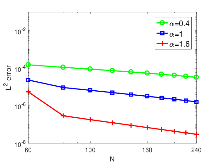
Example 1: Exponential decay $f(x).$ We first consider equation (68) with $f(x)=\exp(-{x^{2}}/{2})(1+x).$ Since the closed-form exact solution is not available, we take the numerical solution with $N=600$ as the reference solution. The convergence results with MMGFs for $\alpha=0.4,1,1.6$ are presented in Figure 1 (middle and right). In the left plot, we have also presented the convergence results for the Hermite function approach in [28]. It is clearly seen that the MMGFs approach outperforms the Hermite approximations for all cases, namely, the MMGFs approach admits much higher convergence rates. This can also be seen form Table 1, where we have presented the order of convergence for both approaches.

Refer to caption — Fig. 1: $L^{2}$ -error with $f(x)=\exp(-{x^{2}}/{2})(1+x)$ . Left: Hermite function approach in [28] with scaling factor $1/0.4$ . Middle: MMGFs approach with $\lambda=0$ and scaling factor $\mu=5$ . Right: MMGFs approach with $\lambda=0.5$ and scaling factor $\mu=5$ .

Table 1: Rate of convergence using the generalized Hermite function, MMGFs with

\lambda=0

, and MMGFs with

\lambda=0.5,

\alpha=1

and

f(x)=\exp(-{x^{2}}/{2})(1+x).

	Hermite		MMGF $\lambda=0$		MMGF $\lambda=0.5$
$N$	$L^{2}$ error	Order	$L^{2}$ error	Order	$L^{2}$ error	Order
60	7.26e-4	–	2.32e-5	–	1.90e-5	–
80	5.72e-4	0.83	1.50e-5	-1.52	1.23e-5	1.50
100	4.77e-4	0.82	1.06e-5	-1.53	8.79e-6	1.51
120	4.09e-4	0.84	8.02e-6	-1.55	6.65e-6	1.53
140	3.58e-4	0.87	6.30e-6	-1.57	5.23e-6	1.56
160	3.17e-4	0.90	5.09e-6	-1.59	4.23e-6	1.59
180	2.84e-4	0.94	4.21e-6	-1.62	3.50e-6	1.62
200	2.57e-4	0.98	3.53e-6	-1.66	2.94e-6	1.66
220	2.32e-4	1.03	3.01e-6	-1.70	2.49e-6	1.71
240	2.12e-4	1.08	2.58e-6	-1.75	2.14e-6	1.77

Example 2: Algebraic decay $f(x).$ We next consider equation (68) with an algebraic decay source term: $f\left(x\right)=\frac{1}{(1+x^{2})^{2}}.$ The plots of the error decay for both Hermite functions and MMGFs are in Figure 2. Indeed, we observe the convergence behaviour similar to the previous example – the MMGF approach has a much better performance. The comparison in Table 2 also shows that the proposed approach converges much faster than the Hermite method.

Table 2: Rate of convergence using the generalized Hermite function, MMGFs with

\lambda=0

, and MMGFs with

\lambda=0.5.

\alpha=1

and

f\left(x\right)=\frac{1}{(1+x^{2})^{2}}

	Hermite		MMGF $\lambda=0$		MMGF $\lambda=0.5$
$N$	$L^{2}$ error	Order	$L^{2}$ error	Order	$L^{2}$ error	Order
60	3.36e-3	–	2.36e-5	–	4.23e-5	–
80	2.61e-3	0.87	9.36e-6	-3.21	2.75e-5	1.49
100	2.17e-3	0.84	6.66e-5	-1.53	1.96e-5	1.51
120	1.86e-3	0.84	5.02e-6	-1.55	1.49e-5	1.53
140	1.63e-3	0.86	3.95e-6	-1.56	1.17e-5	1.56
160	1.45e-3	0.88	3.19e-6	-1.59	9.46e-6	1.59
180	1.30e-3	0.91	2.64e-6	-1.62	7.81e-6	1.62
200	1.18e-3	0.94	2.21e-6	-1.66	6.56e-6	1.66
220	1.08e-3	0.97	1.88e-6	-1.70	5.57e-6	1.71
240	9.84e-4	1.01	1.62e-6	-1.75	4.78e-6	1.77

To better understand the solution behaviours, we present in Figure 3 the asymptotic behavior of the “exact” solutions as $|x|\gg 1$ for the above two examples. We see that, for both examples with very different decay of $f(x)$ , the solution $u(x)$ decays at the same rate: $\lvert x\rvert^{-\alpha-1}$ . This testifies the solution decays at a rate of a power law, as opposite to the usual Laplacian. This also explains the reason why MMGFs have a better performance than the Hermite functions.

6 Modified rational spectral-collocation methods

With the formulas in Theorem 4 at our disposal, we can directly generate the spectral fractional differentiation matrices and develop the direct collocation methods, similar to the Hermite collocation methods in [39]. However, it seems nontrivial and largely open to analyse its convergence. In fact, we can also implement the collocation method in the Fourier transformed domain which turns to be more a natural way to extend the method to multiple dimensions.

6.1 Fractional differentiation matrices

Let $\{x_{j}^{\lambda},\omega_{j}^{\lambda}\}_{j=0}^{N}$ be the mapped Gegenbauer-Gauss collocation points and weights as given in (59). For any $u_{N}\in V_{N}^{\lambda},$ we write

u_{N}(x)=\sum_{j=0}^{N-1}u_{j}l_{j}(x),\quad\textmd{with}\quad l_{j}(x_{k}^{\lambda})=\delta_{jk},\quad 0\leq j,k\leq N-1,

where $u_{j}=u_{N}(x_{j}^{\lambda}).$ Note that the corresponding Lagrange basis function $\{l_{j}(x)\}_{j=1}^{N}$ can be expressed as

l_{j}(x)=\sum_{k=0}^{N-1}\,b_{k}^{j}R_{k}^{\lambda}(x),\quad\textmd{with}\quad b_{k}^{j}=\frac{R_{k}^{\lambda}(x_{j}^{\lambda})\omega_{j}^{\lambda}}{\gamma_{k}^{\lambda}},\quad 0\leq j,k\leq N-1.

Consequently, we can easily derive the associated differential matrix $\mathcal{D}^{L,\alpha,\lambda}$ with Lagrange type bases

\mathcal{D}_{i,j}^{L,\alpha,\lambda}=(-\Delta)^{\alpha/2}l_{j}(x_{i}^{\lambda})=\sum_{k=0}^{N-1}b_{k}^{j}(-\Delta)^{\alpha/2}R_{j}^{\lambda}(x_{i}^{\lambda}),

(73)

where $(-\Delta)^{\alpha/2}R_{j}^{\lambda}(x_{i}^{\lambda})$ can be computed via (26) and (27).

6.2 Numerical examples

We now present several numerical examples to show the performance of the spectral collocation method based on MMGFs. Notice that the collocation method is more practical for problems with variable coefficients and nonlinear problems. Also, we shall carry out comparisons with the Hermite collocation method in [39].

6.2.1 A multi-term fractional model

We first consider the following multi-term fractional Laplacian equation:

\sum_{j=1}^{J}\rho_{j}(-\Delta)^{\alpha_{j}/2}u(x)=f(x),\quad x\in\mathbb{R};\quad u(x)\to 0,\;\;{\rm as}\;\;|x|\to\infty.

(74)

Here we set $J=4$ and

\begin{split}&\alpha_{1}=0,\quad\alpha_{2}=0.5\quad\alpha_{3}=1.5,\quad\alpha_{4}=2,\\ &\rho_{1}=\frac{\pi}{6},\quad\rho_{2}=\frac{\pi}{3},\quad\rho_{3}=\frac{\pi}{3},\quad\rho_{4}=\frac{\pi}{6}.\end{split}

Numerical results with two different souce terms are presented in Figure 4. It can be seen that, similar to the Galerkin methods, the MMGF approach has a much better performance than the Hermite function approach in all cases.

6.2.2 Fractional model with variable coefficients

We next consider the following problem

\begin{split}&(-\Delta)^{\alpha/2}u(x)+r(x)u(x)=f(x),\quad x\in{\mathbb{R}},\\ &u(x)\to 0,\;\;{\rm as}\;\;|x|\to\infty,\end{split}

(75)

where $r(x)=1+\exp(-x^{2})$ and $f(x)=\frac{1}{(1+x^{2})^{1.2}}$ . The convergence results for $\alpha=0.4,1,1.6$ are provided in Figure 5 for both approaches. Again, the MMGFs spectral collocation method outperforms the Hermite collocation method.

6.2.3 An eigenvalue problem

Finally, we consider the following eigenvalue problem as in [39]:

((-\Delta)^{\alpha/2}+x^{2})u(x)=\lambda u(x),\quad x\in{\mathbb{R}}.

(76)

Notice that exact eigenvalues for the case of $\alpha=1$ are available in [26]. For this example, we shall compute the first three eigenvalues by the MMGFs spectral collocation method and the Hermite collocation methods for comparison. The numerical results are given in Figure 6, which shows that the MMGF collocation method is more accurate than the Hermite collocation method.

6.3 Spectral-collocation methods in multiple dimensions

To this end, we propose the modified rational collocation methods based on a formulation in the Fourier transformed domain in multiple dimensions and show that it is more accurate than the Hermite spectral collocation methods in [28].

To fix the idea, we consider the $d$ -dimensional model problem:

\begin{split}&(-\Delta)^{\alpha/2}u(x)+\rho u(x)=f(x),\quad x\in\mathbb{R}^{d};\\ &u(x)\to 0,\quad{\rm as}\;\;|x|\to\infty,\end{split}

(77)

where we denote $x=(x_{1},\cdots,x_{d})$ and $|x|=\sqrt{x^{t}x}.$ It is known that in the Fourier transformed domain, it can be expressed as

(|\xi|^{\alpha}+\rho)\hat{u}(\xi)=\hat{f}(\xi),\quad\xi\in{\mathbb{R}}^{d},

(78)

where $\hat{u},\hat{f}$ are the Fourier transform of $u,f,$ respectively. Thus, we have

\hat{u}(\xi)=\frac{\hat{f}(\xi)}{|\xi|^{\alpha}+\rho},\quad\xi\in{\mathbb{R}}^{d}.

(79)

That is, the Fourier transform of solution $u$ can be expressed explicitly as above. This motivates the construction of the collocation method in the frequency space. To describe the algorithm, we denote

\Upsilon_{\!N}:=\big\{j=(j_{1},\cdots,j_{d})\,:\,j_{i}=0,1,\cdots,N,\;\;1\leq i\leq d\big\},

and define the tensorial grids and tensorial MMGFs as

x_{j}^{\lambda}=(x_{j_{1}}^{\lambda},\cdots,x_{j_{d}}^{\lambda}),\quad j\in\Upsilon_{\!N};\quad R_{n}^{\lambda}(x)=\prod_{i=1}^{d}R_{n_{i}}^{\lambda}(x_{i}).

(80)

As the first step, we approximate $f(x)$ by the multidimensional interpolation:

{I}_{N}^{\lambda}f(x)=\sum_{n\in\Upsilon_{\!N}}\tilde{f}_{n}\,R_{n}^{\lambda}(x),

(81)

where the coefficients $\{\tilde{f}_{n}\}_{n\in\Upsilon_{\!N}}$ can be computed from the samples $\{f(x_{j}^{\lambda})\}_{j\in\Upsilon_{\!N}}$ by the tensorial version of the quadrature (60). Then we have the approximation:

\hat{f}(\xi)\approx\widehat{{I}_{N}^{\lambda}f}(\xi)=\sum_{n\in\Upsilon_{\!N}}\tilde{f}_{n}\,\prod_{i=1}^{d}{\mathscr{F}}[R_{n_{i}}^{\lambda}](\xi_{i}),

(82)

where ${\mathscr{F}}[R_{n_{i}}^{\lambda}](\xi_{i})$ can be computed by the formulas in Theorem 10 below.

Then the direct collocation approximation of $u(x)$ in the frequency space is given by

\widehat{u}_{N}(\xi_{j}^{\lambda})=\frac{\widehat{{I}_{N}^{\lambda}f}(\xi_{j}^{\lambda})}{|\xi_{j}^{\lambda}|^{2}+\rho},\quad j\in\Upsilon_{\!N},

(83)

where $\{\xi_{j}^{\lambda}\}$ are the tensorial grids as in (80). With these samples, we can write the final approximation $u_{N}(x)$ by taking Fourier inverse transform of $\hat{u}_{N}(\xi)$ as follows:

u_{N}(x)=\sum_{n\in\Upsilon_{\!N}}\tilde{u}_{n}\,\prod_{i=1}^{d}{\mathscr{F}}^{-1}[R_{n_{i}}^{\lambda}](x_{i}),

(84)

where the coefficients $\{\tilde{u}_{n}\}_{n\in\Upsilon_{\!N}}$ can be computed from $\{\widehat{u}_{N}(\xi_{j}^{\lambda})\}_{j\in\Upsilon_{\!N}}$ in (83) by the quadrature formula (cf. (60)) as before. Here, the inverse Fourier transforms can be computed by the formulas in Theorem 10 and Remark 6.1 below.

Like Theorem 4, we have the following formulas for computing the Fourier transform of the MMGFs.

Theorem 10.

For real $\lambda>-1/2,$ the Fourier transform of the MMGFs can be computed by

\begin{split}{\mathscr{F}}[R_{2n}^{\lambda}](\xi)&=a_{n}^{\lambda}\sum_{k=0}^{n}\frac{(-n)_{k}(n+\lambda)_{k}}{(\lambda+\frac{1}{2})_{k}\,k!}\frac{|\xi|^{k+\lambda/2}K_{k+\lambda/2}(|\xi|)}{2^{k+(\lambda-1)/2}\Gamma(k+(\lambda+1)/2)},\end{split}

(85)

and

\begin{split}{\mathscr{F}}[R_{2n+1}^{\lambda}](\xi)&=-{\rm i}\,{\rm sign}(\xi)\,b_{n}^{\lambda}\sum_{k=0}^{n}\frac{(-n)_{k}(n+\lambda+1)_{k}}{(\lambda+\frac{1}{2})_{k}k!}\,\frac{|\xi|^{k+\lambda/2}K_{k+(\lambda-1)/2}(|\xi|)}{2^{k+\lambda/2}\Gamma(k+1+\lambda/2)},\end{split}

(86)

where the constants $a_{n}^{\lambda},b_{n}^{\lambda}$ are defined in (21).

Proof.

By (15), we have that for $\gamma>0,$

{\mathscr{F}}\Big[\frac{1}{(1+x^{2})^{\gamma}}\Big](\xi)=\dfrac{2^{1-\gamma}}{\Gamma(\gamma)}|\xi|^{\gamma-\frac{1}{2}}{K_{\gamma-\frac{1}{2}}(|\xi|)},\quad\xi\in{\mathbb{R}}.

Similarly, we derive from (18) that for $\gamma>1/2,$

{\mathscr{F}}\Big[\frac{x}{(1+x^{2})^{\gamma}}\Big](\xi)=-{\rm i}\,\dfrac{2^{1-\gamma}}{\Gamma(\gamma)}\,{\rm sign}(\xi)\,|\xi|^{\gamma-\frac{1}{2}}{K_{\gamma-\frac{3}{2}}(|\xi|)},\quad\xi\in{\mathbb{R}}.

Consequently, the formulas (85)-(86) follow from (3.1)-(3.1) directly. ∎

Remark 6.1.

In (84), we need the inverse transform of $R_{n}^{\lambda}(\xi),$ which can be computed by the same formulas (3.1)-(3.1). Indeed, by definition, we have

{\mathscr{F}}^{-1}[R_{n}^{\lambda}](x)=\frac{1}{\sqrt{2\pi}}\int_{-\infty}^{\infty}e^{{\rm i}x\xi}R_{n}^{\lambda}(\xi)d\xi=\overline{{\mathscr{F}}[R_{n}^{\lambda}](x)}.

(87)

We now consider a two dimensional example with $f(x,y)=\exp(-\sqrt{x^{2}+y^{2}})$ . Notice that the Fourier transform of this source term can be computed as

\displaystyle\mathscr{F}[f](\xi,\eta)=\frac{1}{\left(1+\xi^{2}+\eta^{2}\right)^{3/2}}.

The corresponding numerical results are presented in Figure 7. Once again, the MMGF collocation method is more accurate and converges faster than the Hermite collocation method.

7 Summary and concluding remarks

In this paper, we have developed accurate spectral methods using rational basis (or modified mapped Gegenbauer functions) for PDEs with fractional Laplacian in unbounded domains. The main building block of the spectral algorithms is some explicit formulas for the Fourier transforms and fractional Laplacian of the rational basis. With these, we can construct rational spectral-Galerkin and collocation schemes by pre-computing the associated fractional differentiation matrices. We obtain optimal error estimates of rational spectral approximation in the fractional Sobolev spaces, and analyze the optimal convergence of the proposed Galerkin scheme. Numerical results show that the rational method outperforms the Hermite function approach. Future studies along this line include the error estimates of the rational collocation methods in section 6, fast pre-conditioner/solvers for high dimensional problems, and applications of the MMGFs approach to tempered fractional PDEs.

References

[1] M.S. Agranovich, Sobolev spaces, their generalizations and elliptic problems in smooth and Lipschitz domains, Springer, 2015.
[2] G.E. Andrews, R. Askey, and R. Roy, Special functions (encyclopedia of mathematics and its applications vol 71), 1999.
[3] D.H. Baffet and J.S. Hesthaven, A kernel compression scheme for fractional differential equations, SIAM J. Numer. Anal., 55 (2017), pp. 496–520.
[4] E. Barkai, R. Metzler, and J. Klafter, From continuous time random walks to the fractional Fokker-Planck equation, Phys. Rev. E, 61 (2000), p. 132.
[5] P. Biler, T. Funaki, and W.A. Woyczynski, Fractal Burgers equations, J. Diff. Equat., 148 (1998), pp. 9–46.
[6] A. Bonito, J.P. Borthagaray, R.H. Nochetto, E. Otárola, and A.J. Salgado, Numerical methods for fractional diffusion, Comput. Vis. Sci., 19 (2018), pp. 19–46.
[7] J.P. Boyd, Spectral methods using rational basis functions on an infinite interval, J. Comput. Phys., 69 (1987), pp. 112–142.
[8] J.P. Boyd, Chebyshev and Fourier Spectral Methods, Dover Publications Inc., Mineola, NY, second ed., 2001.
[9] J.Y. Cao and C.J. Xu, A high order schema for the numerical solution of the fractional ordinary differential equations, J. Comput. Phys., 238 (2013), pp. 154–168.
[10] S. Chen, J. Shen, and Z. Mao, Efficient and accurate spectral methods using general Jacobi functions for solving Riesz fractional differential equations, Appl. Numer. Math, 106 (2016), pp. 165–181.
[11] S. Chen, J. Shen, and L.L. Wang, Generalized Jacobi functions and their applications to fractional differential equations, Math. Comp., 85 (2016), pp. 1603–1638.
[12] , Laguerre functions and their applications to tempered fractional differential equations on infinite intervals, J. Sci. Comput., 74 (2018), pp. 1286–1313.
[13] A. de Pablo, F. Quirós, A. Rodríguez, and J.L. Vázquez, A fractional porous medium equation, Adv. Math., 226 (2011), pp. 1378–1409.
[14] J.C.M. Fok, B.Y. Guo, and T. Tang, Combined Hermite spectral-finite difference method for the Fokker-Planck equation, Math. Comp., 71 (2002), pp. 1497–1528 (electronic).
[15] I.S. Gradshteyn and I.M. Ryzhik, Table of integrals, series, and products, translated from the russian, translation edited and with a preface by daniel zwillinger and victor moll, revised from the seventh edition, 2015.
[16] B.Y. Guo, J. Shen, and Z.Q. Wang, A rational approximation and its applications to differential equations on the half line, J. Sci. Comp., 15 (2000), pp. 117–147.
[17] B.Y. Guo and Z.Q. Wang, Modified Chebyshev rational spectral method for the whole line, in Proceedings of the fourth international conference on dynamical systems and differential equations, 2002, pp. 365–374.
[18] Y.H Huang and A. Oberman, Numerical methods for the fractional Laplacian: A finite difference-quadrature approach, SIAM J. Numer. Anal., 52 (2014), pp. 3056–3084.
[19] C.C. Ji and Z.Z. Sun, A high-order compact finite difference scheme for the fractional sub-diffusion equation, J. Sci. Comput., 64 (2015), pp. 959–985.
[20] B.T. Jin, R. Lazarov, and Z. Zhou, Error estimates for a semidiscrete finite element method for fractional order parabolic equations, SIAM J. Numer. Anal., 51 (2013), pp. 445–466.
[21] E. Kharazmi, M. Zayernouri, and G.E. Karniadakis, Petrov–Galerkin and spectral collocation methods for distributed order differential equations, SIAM J. Sci. Comput., 39 (2017), pp. A1003–A1037.
[22] H. Khosravian-Arab, M. Dehghan, and M.R. Eslahchi, Fractional Sturm–Liouville boundary value problems in unbounded domains: Theory and applications, J. Comput. Phys., 299 (2015), pp. 526–560.
[23] N.S. Landkof, Foundations of modern potential theory springer, New York, (1972).
[24] J.L. Lions and E. Magenes, Non-homogeneous boundary value problems and applications, Vol. II. Die Grundlehren der mathematischen Wissenschaften. Springer-Verlag, New York-Heidelberg, (1972).
[25] A. Lischke, M. Zayernouri, and G.E. Karniadakis, A tunably-accurate laguerre petrov-galerkin spectral method for multi-term fractional differential equations on the half line, arXiv preprint arXiv:1607.08579, (2016).
[26] J. Lorinczi and J. Malecki, Spectral properties of the massless relativistic harmonic oscillator, arXiv preprint arXiv:1006.3665, (2010).
[27] H.P. Ma, W.W. Sun, and T. Tang, Hermite spectral methods with a time-dependent scaling for parabolic equations in unbounded domains, SIAM J. Numer. Anal., 43 (2005), pp. 58–75.
[28] Z.P. Mao and J. Shen, Hermite spectral methods for fractional PDEs in unbounded domains, SIAM J. Sci. Comput., 39 (2017), pp. A1928–A1950.
[29] F.W.J. Olver, D.W. Lozier, R.F. Boisvert, and C.W. Clark, NIST handbook of mathematical functions cambridge university press, New York, (2010).
[30] Y. Ren, X. Yu, and Z.Q. Wang, Diagonalized Chebyshev rational spectral methods for second-order elliptic problems on unbounded domains, Numer. Math. Theor. Meth. Appl, 12 (2019), pp. 265–284.
[31] J. Shen, T. Tang, and L.L. Wang, Spectral methods: algorithms, analysis and applications, vol. 41, Springer, Berlin, 2011.
[32] J. Shen and L.L. Wang, Some recent advances on spectral methods for unbounded domains, Commun. Comp. Phys., 5 (2009), pp. 195–241.
[33] J. Shen, L.L. Wang, and H.J. Yu, Approximations by orthonormal mapped Chebyshev functions for higher-dimensional problems in unbounded domains, J. Comput. Appl. Math., 265 (2014), pp. 264–275.
[34] C.T. Sheng and J. Shen, A hybrid spectral element method for fractional two-point boundary value problems, Numer. Math. Theor. Meth. Appl., 10 (2017), pp. 437–464.
[35] , A space-time Petrov-Galerkin spectral method for time fractional diffusion equation, Numer. Math. Theor. Meth. Appl, 11 (2018), pp. 854–876.
[36] F.Y. Song, C.J. Xu, and G.E. Karniadakis, Computing fractional Laplacians on complex-geometry domains: algorithms and simulations, SIAM J. Sci. Comput., 39 (2017), pp. A1320–A1344.
[37] T. Sun, R. Liu, and L.L. Wang, Generalised Müntz spectral Galerkin methods for singularly perturbed fractional differential equations, East. Asia. J. Appl. Math., 8 (2018), pp. 611–633.
[38] T. Tang, The Hermite spectral method for Gaussian-type functions, SIAM J. Sci. Comput., 14 (1993), pp. 594–606.
[39] T. Tang, H.F. Yuan, and T. Zhou, Hermite spectral collocation methods for fractional PDEs in unbounded domains, Commun. Comput. Phys., 24 (2018), pp. 1143–1168.
[40] W.Y. Tian, H. Zhou, and W.H. Deng, A class of second order difference approximations for solving space fractional diffusion equations, Math. Comp., 84 (2015), pp. 1703–1727.
[41] T.Tang, H. Yu, and T. Zhou, On energy dissipation theory and numerical stability for time-fractional phase field equations, arXiv:1808.01471, (2018).
[42] Z.Q. Wang and B.Y Guo, Modified Legendre rational spectral method for the whole line, J. Comput. Math., (2004), pp. 457–474.
[43] S.L Wu and T. Zhou, Fast parareal iterations for fractional diffusion equations, J. Comput. Phys., 329 (2017), pp. 210–226.
[44] , Parareal algorithms with local time-integrators for time fractional differential equations, J. Comput. Phys., 385 (2018), pp. 135–149.
[45] X.Guo, Y. Li, and H. Wang, A fast finite difference method for tempered fractional diffusion equations, Commun. Comput. Phys., 24 (2018), pp. 531–556.
[46] Y.Yang and H.Ma, The legendre Galerkin-Chebyshev collocation method for space fractional Burgers-like equations, Numer. Math. Theor. Meth. Appl, 11 (2018), pp. 338–353.
[47] M. Zayernouri and G.E. Karniadakis, Fractional Sturm–Liouville eigen-problems: theory and numerical approximation, J. Comput. Phys., 252 (2013), pp. 495–517.