Rethinking Arithmetic for Deep Neural Networks
Abstract
We consider efficiency in the implementation of deep neural networks. Hardware accelerators are gaining interest as machine learning becomes one of the drivers of high-performance computing. In these accelerators, the directed graph describing a neural network can be implemented as a directed graph describing a Boolean circuit. We make this observation precise, leading naturally to an understanding of practical neural networks as discrete functions, and show that so-called binarised neural networks are functionally complete. In general, our results suggest that it is valuable to consider Boolean circuits as neural networks, leading to the question of which circuit topologies are promising. We argue that continuity is central to generalisation in learning, explore the interaction between data coding, network topology, and node functionality for continuity, and pose some open questions for future research. As a first step to bridging the gap between continuous and Boolean views of neural network accelerators, we present some recent results from our work on LUTNet, a novel Field-Programmable Gate Array inference approach. Finally, we conclude with additional possible fruitful avenues for research bridging the continuous and discrete views of neural networks.
Notation
denotes the reals, and the set of Boolean truth values, where denotes false and denotes true. is used to denote the rectified linear unit function . denotes the sigmoid function . We denote function composition by . denotes the set of all functions from to . The set of integers is denoted by , and the set of integers bounded in absolute value by . The following Boolean connectives are used: denotes negation, denotes conjunction, denotes disjunction, and denotes exclusive or (XOR).
1 Introduction
This paper considers the development of deep neural networks in the supervised learning setting [1]. Inspired by the recent rise of interest in specialised hardware accelerators for deep neural networks [2], we shall take a fresh look at the question of suitable network topologies and basic node functionalities for such accelerators.
We shall begin by defining the supervised learning problem. Let denote the set of possible inputs to a machine learning inference function, and denote the set of possible outputs. Imagine that we have an oracle function , mapping every possible input to the corresponding ideal output . Generally, we will be interested in inference via a family of parametrically-defined functions , with parameters drawn from some set . We will often write when we wish to consider the case where the parameter value has been fixed. These functions will not, in general, produce the ideal output for all possible inputs, and therefore we need to consider some notion of inaccuracy, or ‘loss’, , which measures the difference between the ideal output and the actually computed output as . For simplicity, we assume in this article that is a metric [3] defined on . We are generally interested in average-case behaviour of these parametric functions ‘in the wild’, on any data that may frequently appear as input in real usage. Lifting the metric on to the following metric defined on functions ,
| (1) |
where the expectation is over the input space, we can then pose the question of supervised training as the following optimisation problem of selecting parameters to minimize distance to an oracle function:
| (2) |
There are some practical problems, however. Firstly, it is unlikely that we have access to or knowledge of the distribution of or to an oracle function , except through a finite set of samples, known as the training set. Secondly, as Scheinberg notes [4], the loss function desired in practice (e.g. an indicator function) may give rise to a computationally intractable optimisation problem. As a result, it is common to aim instead to solve the training problem,
| (3) |
where are the training data – inputs for which the ideal output is known – and is some suitable, often convex, loss function.
The actual accuracy of the resulting function , can then be evaluated on some other set of data – the test data, as a proxy for , to obtain the test error:
| (4) |
It turns out that this setting therefore imposes particular restrictions on the family of parameterised functions , because we wish – which was selected based only on the training data – to also work well for the test data, as well as ensuring several other properties to be discussed. This fundamental problem: the design of families of parameterised functions for this purpose, is the key subject of study of this paper. In particular, we address here the case where the functions map from one finite set to another, which is always the practical setting in a finite-precision computer. By considering the discrete problem explicitly, several new insights are developed, which may be of value to those researching highly-efficient machine inference.
The structure of this paper is as follows:
Section 2 introduces a model of computation defined by typed graphs. We use this model to develop a deeper understanding of the computation of inference functions in deep neural networks, discussing suitable choices for such functions. The model also lets us reason about their approximation by discrete functions, and hence the potential for hardware implementations of such computations. In Section 3, we present an abstract view of the typical digital design process for hardware accelerators of numerical functions. We then show that a known family of extremely quantised neural networks is functionally complete. This result runs counter to standard thinking in hardware-accelerated neural networks, and we shall consider the reason for this apparent contradiction. Section 4 revisits the question of appropriate inference functions from Section 2, but now in the discrete setting. We argue for a trinity of topology, node functionality and metrics as interacting to determine efficient inference computation, and pose some open questions regarding the extent to which these factors can be decoupled. In Section 5, we consider an approach for efficient FPGA inference, known as LUTNet, recently published by my research group as an example of initial work bridging the continuous and discrete setting. Finally, Section 6 draws conclusions and points to several fruitful avenues for further research.
2 Networks and Inference Functions
A Graphical Approach
A graphical approach is universally used to describe – formally or informally – the computations performed by deep neural networks. In this section we shall develop a slightly unorthodox but very general formalism, which will be of use throughout the paper. Our aim here is to distinguish the syntactic description of neural networks as graphs from the semantic interpretation as functions. This distinction will be important because the transformations applied to develop a realisation of a neural network as a program or a piece of digital hardware are primarily based on the syntactic representation.
Definition 2.1.
An edge is simply a unique label, together with a set such as or , which can be interpreted as the type of data carried by the edge in a network.
Example 2.1.
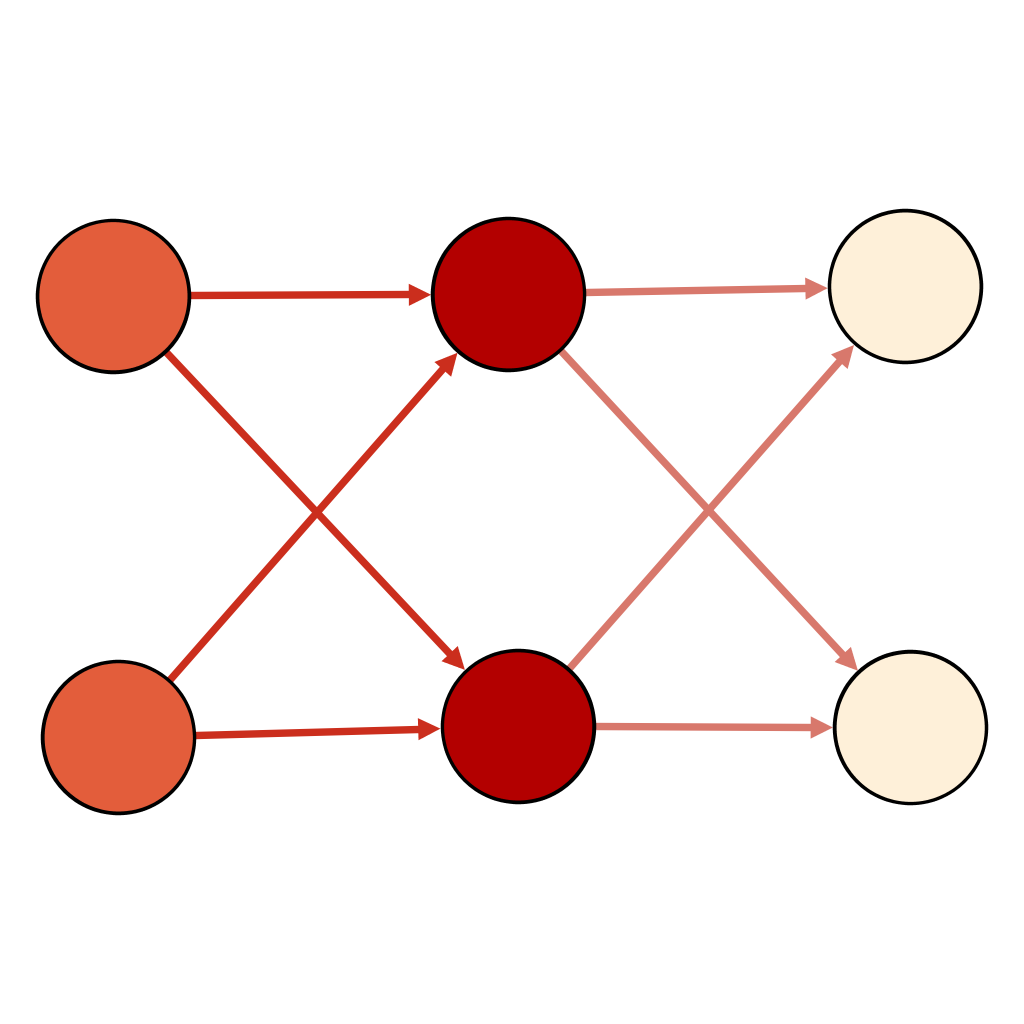
In Fig. 1, , , , , and are all edges, which we will take to be of real type.
Definition 2.2.
A vertex is a tuple of ordered lists of edges param, in and out, together with a function func from the Cartesian product of the sets defined by param and in to that of those defined by out.
Example 2.2.
In Fig. 1, there is a vertex .
The purpose of distinguishing param from in is to identify those values (parameters) that are intended to be determined once, offline, versus those values (activations) that are intended to be change each time the graph is used in inference – we use a semicolon to separate parameters from activations, for readability purposes. In this example, and are parameters, commonly called weights, while and are not. There is one other vertex shown in the figure; this vertex has an empty parameter list.
Definition 2.3.
A network is a pair of vertices together with a distinguished set of edges priout such that:
- •
No edge appearing in the param list of any vertex also appears in the out list of any vertex.
- •
No edge appears in the out list of more than one vertex.
- •
All edges in priout appear in the list out list of exactly one vertex.
We will refer to parameters of the network to mean the list of all edges appearing in the param list of any vertex; inputs to the network to mean the list of all edges appearing in the in list of some vertex but not in the out list of any vertex; and outputs of the network to be the set priout. We will often refer to the ‘leaf functions’ of a network, meaning the collection of functions func of all the vertices in the network.
Example 2.3.
The network shown in Fig. 1 consists of the two vertices previously described, together with a set of primary outputs. One possibility for such a set is , but there are other choices, depending on which edges are required to be observable at the network output. The parameters of this network are and , and the inputs to the network are and .
Definition 2.4.
We say that a network implements a function defined through the natural function composition of the individual vertex functions, i.e. is a function from the Cartesian products of parameters and inputs of the network to the Cartesian product of the outputs of the network, defined inductively, with vertex functions as the leaf functions.
Example 2.4.
For the network shown in Fig. 1, .
For simplicity, we will consider computations corresponding to acyclic networks – including the very significant class of Convolutional Neural Networks [5] – however the formalism can easily be extended to cyclic networks (e.g. LSTMs [6]) by lifting computation over the types illustrated above to computations over streams of those types [7]. This generalisation does not affect the following material. Equally, it is trivial to make networks hierarchical by generalising functions computed to also allow sub-networks, but this will not be required in the sequel.
Functions for Inference
What kind of functions form good candidates for machine learning? And what basic functionality should be implemented by nodes in a network for this purpose? In practical terms, for deep learning today, the most common leaf functions are inner products, ReLU, sigmoid, and softmax [1]. However, it is worth considering the various factors that determine this choice now and in the future. Informally, functions should:
- ❶
Generalise well: once the parameter is selected based on training data, should also tend to perform well over unseen test data.
- ❷
Be cheap to compute: the cost (speed, energy) of evaluating the function at inference time should be low.
- ❸
Be sufficiently general / expressive: the functions should be capable of approximating a wide variety of oracle functions .
- ❹
Be easy to learn: optimisation algorithms used to address the training problem described in Section 1 should be both cheap to execute and also rarely give rise to values of parameter that are grossly suboptimal with respect to the training set.
Strang [8] argues that continuous piecewise linear (CPL) functions have tended to perform well, explaining the importance of inner product and ReLU functions in today’s networks, as CPL functions are precisely those that are implemented by networks with these vertices. Strang argues that continuity is key to generalisation, which intuitively makes sense: if an untrained input is very close to a trained one, it seems reasonable to expect the corresponding outputs of the network to be very close in turn.
To make this intuition precise requires us to equip the input and output sets with metrics, and , respectively, allowing us to define what it means for inputs and outputs to be ‘close’. We can then consider the inference function as a function from an input metric space to an output metric space . We have a choice of options to define continuity; we shall use Lipschitz continuity [3], for reasons that will become apparent in the next section.
Definition 2.5.
Suppose , where is equipped with a metric and is equipped with a metric . Let . The function is -Lipschitz if for all , .
Definition 2.6.
A function is Lipschitz if it is -Lipschitz for some .
Example 2.5.
For computation over with metrics determined by a suitable norm in that space, the ReLU function is Lipschitz and inner products are Lipschitz, and thus by composition, networks constructed from these two functions are Lipschitz [3] and therefore good candidates for generalising beyond training data.
Whether inner products and ReLU functions are cheap to compute (Property ❷) depends upon our model of computation; in the abstract Blum-Shub-Smale model for real computation, this is certainly the case [9]. It is now well-known that a wide variety of neural networks, including those implementing CPL functions are universal approximators, and hence sufficiently general [10, 11] (Property ❸). This leaves the question of whether such functions are ‘easy to learn’ (Property ❹). This is still an active area of research, however theoretical insights such as [12] combined with practical experience suggest that this is indeed the case.
So while CPL functions over the reals appear to be very promising, practical computers do not compute over the reals. In practice, finite precision datatypes are (almost) always used to approximate computation over the reals, and the picture of appropriate inference functions has the potential to change considerably in this setting. We examine this question in this next section.
3 Discrete Inference
We shall refer to a network where the types of all activations are as a real network, where the types of all activations are for finite as a finite-precision network, and where the types of all activations are as a Boolean network. Boolean networks correspond exactly to combinational digital circuits, and so hold a special place from an implementation perspective.
Figure 2 illustrates the standard digital design process for development of a Boolean network approximating a given real network . The first step is that of quantisation. Here, real data types associated with edges in are replaced by finite precision data types . Typical examples are single-precision IEEE floating point arithmetic [13] as well as various fixed-point arithmetics. Consequently, the functions func performed by each node in the network must also be quantised, hence it is common to require ’s node functions to be drawn from a basic set of operators for which this function quantisation process can be performed automatically or is defined by some standard as, e.g. are for IEEE floating-point arithmetic. The quantisation process induces a change in function: in general, and so has been the subject of a considerable amount of work in the DNN literature, with modern machine inference architectures often offering choices of precision that trade performance for accuracy of computation [2], e.g. [14]. The main distinguishing features of this setting compared to classical finite precision quantisation results [15] are due to the metric introduced in Section 1: both its inherently stochastic nature and distance to an oracle rather than distance to the underlying real function being the primary concern, i.e. the ideal quantisation is one that by selecting minimises rather than . In practice, however, it is typical to initially select the each element of the quantised parameter independently, effectively relying on repeated application of the triangle inequality applied syntactically to the graph to ensure remains small, further relying on the triangle inequality property of to ensure the distance to the oracle does not grow considerably. Sometimes this initial choice is refined through a process known as re-training [2].
The second step of the process is to convert the finite-precision network to a Boolean network for implementation. This process is fully automated in modern digital design tools. Firstly, each vertex in the finite-precision graph is replaced by a Boolean network defined for that particular node’s function, for a pre-defined encoding of the elements of into elements of , e.g. the IEEE floating-point storage standard [13] which encodes each single-precision floating point number as a -bit vector of Boolean values; this part of the process is known in digital design as ‘core generation’. Secondly, logic synthesis tools [16] are applied to rewrite the graph to reduce its implementation cost as a circuit. The result of this process is a Boolean network which can be directly implemented as a digital logic circuit. The computation implemented by corresponds exactly to that implemented by in the sense that , where denotes the restriction of the function to the domain of , i.e. the middle section of the diagram commutes.
It can therefore be seen that in a standard digital design process, the only part of the process where an approximation is induced (the upper section of Fig. 2) is not associated with topological changes to the network, while the only part of the process where topological changes are induced (the middle section of Fig. 2) is not associated with approximation. This observation will be of importance in the sequel.
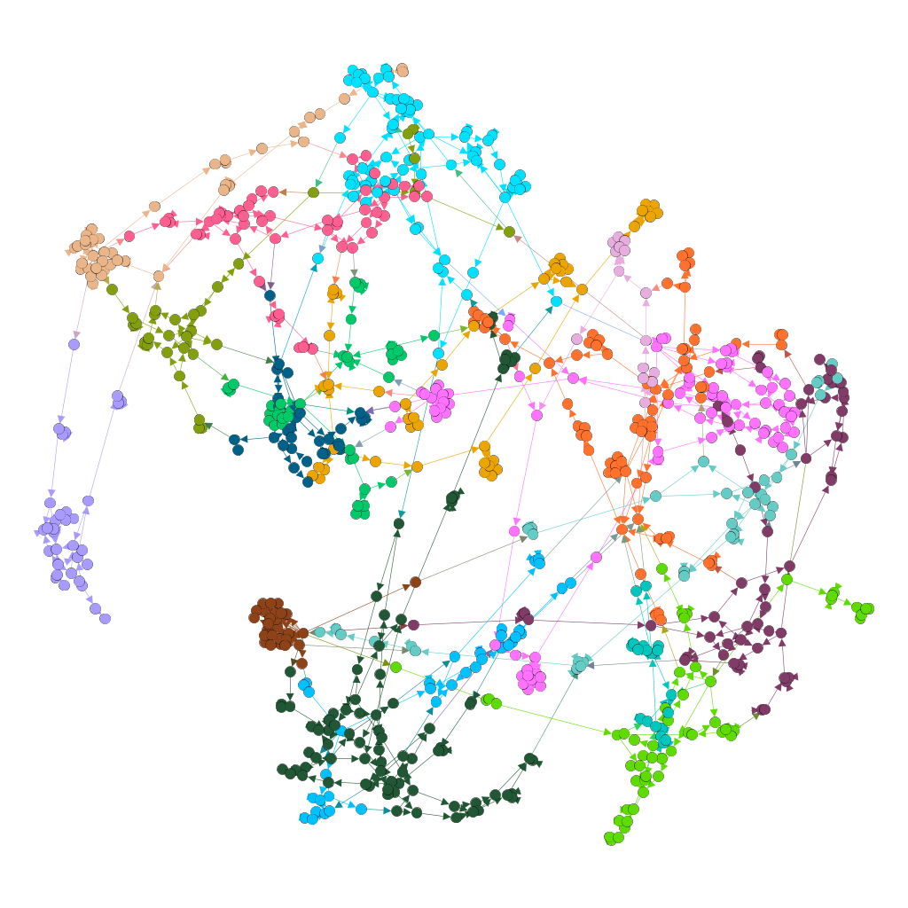
The abstract process described in Fig. 2 is illustrated for a concrete example in Figure 3. The small inset figure corresponds to the topology of , the original specification graph, where each vertex is associated with a function given by . Fixing and to specific values, quantising the computation to a 4-bit fixed-point arithmetic, and synthesising the result produces the large main figure, corresponding to , where each vertex is associated with a 1- or 2-input Boolean function. Clearly there are some key differences between these networks apart from their datatypes: has an irregular structure compared to and has clusters of tightly interconnected ‘neighbourhoods’, roughly corresponding to the Boolean networks introduced for each fixed-point arithmetic function in . However, by maintaining the entire design process within the same graph formalism, we can also exploit the similarities: both are directed graphs operating on typed data, with nodes which can be considered as parametric functions - for the real network the parametric functions are dot products with parameters given by weights, for the Boolean network they are Boolean functions with the parameter indicating which function from or has been selected by the logic synthesis tool.
Binarised Neural Networks
Driven by the desire to reduce energy consumption and improve performance as much as possible, an extreme form of fixed-point arithmetic has been used in so-called binarised neural networks (BNNs) [19]. In these neural networks, both the weights and the activation signals are constrained to be drawn from , resulting in extremely efficient implementations [20]. A classical function given by implemented by component of a deep-neural network, is aggressively quantised to given by for , and otherwise. The key to the implementation efficiency of such functions comes from the near-elimination of hardware-expensive multiplication operations: multiplication in a vector scalar product is reduced to a Boolean exclusive (XNOR) function. Meanwhile, the addition in the scalar product is reduced to calculation of Hamming weight (population count), which admits efficient implementations [21].
Although BNNs have received a lot of attention, the general view in the implementation community is that neural networks constructed in this way are not universally able to implement as good quality classification on complex data sets compared to more precise data representations. This observation has led to manufacturers including configurable finite-precision datapaths typically down to 4-bit [14] or 8-bit [22]. It is instructive to pursue an alternative view, which we shall now develop.
Definition 3.1.
A set of Boolean functions is functionally complete if every Boolean function can be obtained as a finite composition of these functions[23].
Through an appropriate pair of encodings , and , it therefore follows that any function between finite sets can be implemented by a Boolean network using a functionally complete set of Boolean functions at its vertices, similarly to Fig. 2, i.e. for some Boolean network .
Theorem.
The set of node functions in a Boolean implementation of Binarized Neural Networks is functionally complete.
Proof.
We shall use the bijection defined by , . Clote and Kranakis [23] provide necessary and sufficient conditions for a set of Boolean functions to be functionally complete; one well-known such set is , together with the constants and . The equivalences below can easily be shown through enumeration:
| (5) |
∎
Note that it is therefore always possible to construct a real-valued DNN which, when quantised to produce a BNN, implements any Boolean function, including those Boolean functions that would have been derived via traditional design techniques (Fig. 2) using any finite-precision datatype , i.e. BNNs easily satisfy our Property ❸. The theorem therefore challenges received wisdom that binarised neural networks are not always able to produce the required accuracy on a classification task. So why this apparent discrepancy in practice? The issue is not with the computational generality of BNNs, but rather with the traditional design technique, which is unable to adapt the topology of the network to the requirements of the underlying datatype.
Corollary.
Accuracy-optimal network topology depends on finite-precision datatype.
This corollary leads to a conjecture on future design methods for efficient neural networks, which generalises some empirical observations, e.g. that reducing precision can be compensated by increasing network depth [24] or width [25]. Today, digital circuits are universally implemented using CMOS technology [26], whether in a microprocessor or a custom circuit design. CMOS circuits form extremely efficient implementations of nonlinear operations with a single output bit. This contrasts sharply with the standard nodes of real-valued DNNs, the inner product and the ReLU, which are piecewise linear but arbitrarily precise. The usual approach to this dichotomy is to use wide enough finite-precision datatypes to make the hardware emulate the real-valued model: but at what cost?
Conjecture.
Future efficient neural network topologies will be driven by both the topology of the data and by the nature of the discrete representation of the activations. The current separation between approximation (without topological changes) and topological changes (without approximation) will not survive the drive for efficient computation.
4 Boolean Networks for Lipschitz Functions
Since we have demonstrated the link between topology and data representation in deep neural networks, a natural question arises: which topologies may form good choices for learning Boolean functions? Perhaps one may even remove the level of abstraction in Fig. 2, which would then become equivalent to learning the arithmetic.
In Section 2, we discussed the properties of inference functions in a continuous setting; we shall now extend this discussion to Boolean networks. The aim of this section is to focus on Property ❶: how can we develop Boolean networks exhibiting good generalisation?
We explained, following Strang, the centrality of continuity to generalisation in Section 2. The advantage of working with Lipschitz continuity is that we can directly transfer this idea to the Boolean setting. Here, every function is Lipschitz, since we may take the Lipschitz constant , so it is not meaningful to talk about continuity in absolute terms, but rather about the value of the Lipschitz constant. We shall therefore study the question which Boolean networks give rise to -Lipschitz functions? The intuition here is that the lower the Lipchitz constant, the better the function meets the desirable property that small input perturbations cause at most small output perturbations.
Before investigating a concrete example of a simple Boolean circuit in this context, let us consider typical ways to define a metric on the Boolean vectors forming the inputs and outputs of a circuit. It will be helpful to define as , . Although not strictly necessary, it is typical to consider metrics induced by norms of encoded data, e.g. for the domain, where . Here we may interpret as denoting a real vector represented by the Boolean inputs. A trivial example would be , a representation of a two-bit scalar integer in standard binary arithmetic. A more complex scalar encoding corresponds to IEEE single or double-precision floating point, as explicitly given in the standard [13].
It is instructive to consider the most basic typical arithmetic circuit, known as a ripple-carry adder, shown in Fig. 4[27]. Each leaf node implements a Boolean function known as a full adder: , where denotes Boolean XOR. We can consider this circuit as implementing a function . If we define as the function mapping vectors of Boolean values to the number they represent in a standard binary integer encoding:
| (6) |
, then it can be seen why the Boolean network is referred to as an adder: , where denotes standard integer addition. In the formalism of Fig. 2, , .
Let us equip the input and output spaces with suitable metrics, e.g. those induced by the 1-norm of the difference in their word-level representation:
| (7) |
Lemma.
The function implemented by a ripple-carry adder is -Lipschitz for any .
Proof.
| (8) |
∎
How does this -Lipschitz property arise? Note that from the topology of the network alone, we cannot conclude anything useful about the minimal Lipschitz constant of the function implemented; replacing the function of the leaf nodes with an alternative function results in a minimal Lipschitz constant of rather than . Changing the metrics – equivalent in the norm-induced case to encoding the input or output with a different number system – could equally impact on the Lipschitz properties. Finally, a different network topology based on the same full-adder leaf nodes could clearly lead to a different minimal Lipschitz constant. Thus the minimal Lipschitz constant exhibited by a function implemented by a network will generally depend on three things: the topology of the network, the leaf-node functionality, and the encoding / metrics associated with the inputs and outputs of the network. Even if we assume the latter to be fixed, the interaction between the former two features is not ideal if we wish to learn the functionality of nodes in the network: local decisions on Boolean functionality can potentially have global impact on generalisation behaviour of a network.
Learning from the -bit adder example, one natural approach to generating functions with low Lipschitz constant appears to be to reverse the direction of the ‘carry’ edges . If these edges are reversed, then no path exists between , , and or for any , meaning that changes in low-significance input bits cannot impact high-significance output bits. This topology is also appealing because it corresponds directly to most-significant-digit-first arithmetic, a universal approach to computation pioneered by Ercegovac [28] in the 1970s for computer arithmetic: through a suitable change in the encoding , this topology can be utilised to implement all the basic arithmetic operators [29]. However, such a topology does not guarantee a particular Lipchitz constant for the metrics defined in (8), because small changes in the input metric can still correspond to large changes in the most-significant-digit: one sees this for example with the transition , a change of one but with a most-significant-digit bit flip. To avoid this issue, one must either change the encoding of the network inputs and outputs or place restrictions on the Boolean functionality of the nodes. The former approach – selecting an optimal encoding of the input space as Booleans – is an open problem. A trivial but inefficient solution would be to utilise a unary encoding. More efficient solutions could potentially draw deeply from the area of combinatorial Gray codes [30], i.e. methods for generating combinatorial objects (such inputs of a discrete-valued neural network, drawn from ), so that successive objects differ by a small degree. As noted by Savage [30], Gray codes are not preserved under bijection, and it is exactly this property that could suggest implementation-appropriate coding.
Open Problem 1.
For future deep neural networks, what input and output codings are commensurate with the properties of good inference functions identified in Section 2, and how do they depend on the input probability space and oracle function?
The author performed the following simple experiment to investigate the latter approach, i.e. restricting Boolean functionality to ensure a certain Lipschitz constant for fixed topology and metrics. Consider the simple topology shown in Fig. 4(b) with associated metrics and . There are choices for the Boolean functionality of . If we assume that neither constant functions nor those in are of interest, then there are choices for each of and . A complete enumeration identifies 376 pairs of Boolean functions , for which the network implements a 2-Lipschitz function. One may go further and ask whether we can identify a set of choices for the function of and the function of such that we may arbitrarily choose functions from these two sets while maintaining the 2-Lipschitz property, effectively decoupling the choice of leaf functionality from topology. We shall refer to such sets as a ‘functional decoupling’ for given topology, value of , and metrics.
Definition 4.1.
Given a network with enumerated vertices , implementing a -Lipschitz function , a functional decoupling is a tuple of sets such that for every vertex, may be replaced by any element of independently, while maintaining the -Lipschitz property.
Consider a bipartite graph with node set , where is in one-to-one correspondence with the set of choices for function and similarly for function , and in which edges correspond to the pairs of functions resulting in a network implementing a 2-Lipschitz function. A biclique [31] of this graph corresponds to a decoupled set. Using the algorithm of Gillis and Gilneur [32] reveals such a biclique of size for this topology11 1 Code at: https://github.com/constantinides/rethinking, i.e. any combination of these choices of node function results in a 2-Lipchitz network function.
Open Problem 2.
Given metrics on input and output, a Lipschitz constant , and a network topology, is there a useful characterisation of exactly which functions can be implemented by a network with this topology using only leaf functions drawn from functional decouplings?
The significance of this problem is that it would help us to characterise the extent to which it is useful to consider promising network topologies separately from leaf functions.
5 The Discrete-Continuous Divide: Preliminary Work
One of today’s most promising platforms for practical realisation of very high performance deep neural networks today is the Field-Programmable Gate Array (FPGA) [33]. These architectures provide an interesting case study for exploring some of the ideas presented in this paper, because there is a natural choice for the set of leaf functions implemented in a network: the set [23] of -input Boolean functions, where is a device-specific parameter. This is a natural choice because the underlying architecture is actually built of small physical Boolean lookup tables, each programmable to implement any one of the functions in , together with programmable interconnect able to connect these lookup tables in an effectively arbitrary topology ( is common).
Wang et al. [34] have recently begun to explore the potential for making use of the additional flexibility provided by these lookup tables. In this initial work – which we call LUTNet – we begin by taking a reasonably traditional approach, following [35]: some standard DNN benchmarks from the literature are quantised to use single-bit weights from , and retrained to improve classification accuracy. In the resulting network, many of the vertices have function , usually as part of the standard inner product common in DNNs. We observe that such computation is inefficient, because the basic lookup tables are not being used to their full potential: in the extreme, we have hardware capable of implementing any function from used solely to implement 2-input XNOR gates. We therefore modify the network in the following way. Firstly, we replace the vertex functions given by by the strictly more general class of functions consisting of all functions (isomorphic to) , where the parameter selects the particular function. To make use of the additional support of these functions ( two-valued activations rather than just one), we heuristically allocate the additional inputs to connect to other nodes in the network with low values of weight before quantisation. After initially setting the new functions to reproduce the original, i.e. selecting the parameters from to be precisely those regenerating the function , we then retrain the network using standard Stochastic Gradient Descent (SGD) methods. Finally, we simplify the network topology through a standard ‘pruning’ technique [36]. The intuition of this process is that the nonlinear generality of the class may compensate for the pruning, resulting in a higher accuracy for a given number of Boolean network nodes. This is indeed what we observe in Fig. 5, which represents the classification error rate on the test set versus network area (in LUTs) for classification the CIFAR-10 [37] dataset containing 60,000 32x32 colour images of 10 different classes, using the CNV neural network model [20] as the baseline topology from which the modifications described above are made to the largest layer - in the case of CNV, this is a sizeable convolutional layer with 256 outputs, operating with 3x3 kernels [34]. For this network, we see a reduction in area consumption of approximately 50% compared to the baseline implementation operating at the same classification accuracy.
Using SGD in this discrete setting requires a lifting to a continuous interpolation, as described in detail in [34]. LUTNet is thus representative of one way direction in which to cross the discrete-continuous divide; some possible approaches to crossing in the opposite direction are explored in Section 6.
6 Future Directions
It is the central thesis of this paper that there is much to learn by viewing neural networks and digital circuits as two embodiments of typed operations on graphs.
The topic of determining a good neural network topology is still in its infancy [1]. We have shown that there are additional dimensions to this problem: finite-precision data representation and the metrics determining ‘closeness’ of input and output also have a direct impact on efficient network topologies. Coupling these two concerns would seem to be a significant avenue for fruitful research in deep learning.
While the literature on learning appropriate parameters for predefined neural network topologies has developed rapidly in recent years [1], systematic algorithmic approaches to learn neural network topologies from data are only recently appearing [38] and the underlying theory is limited. This mirrors the situation in automated synthesis of digital circuits before the 1990s: the automated synthesis of logic circuits consisting of two layers (one of AND gates with optional input inversion, followed by one of OR gates) had been understood theoretically [39] and practically [40] before the 1990s, but only during that decade did the technology to optimise multi-level (’deep’) Boolean networks emerge [16]. There may be considerable scope for crossover between the electronic design automation community and the deep learning community based on this work. Recently, there has been a resurgence of interest in the problem of exact (i.e. optimal) logic synthesis [41], which – albeit it in a different setting – also needs to simultaneously explore topology and node functionality, and is stymied by the resulting computational complexity. This suggests a possible avenue for future development is to lift the progress being made in this area to richer data types.
The problem of placing bounds on the number of graph nodes drawn from a certain basis set required to meet a given quality of classification, e.g. via metric (1), could potentially be a very interesting topic for further theoretical study. There is a rich literature on circuit complexity bounds [23], and it may be possible to combine these ideas with probabilistic notions from Minimum Length Descriptions [42] to bound minimal circuit sizes22 2 The latter interesting suggestion originated from an anonymous reviewer of the original manuscript..
The -Lipschitz property used in this paper is a global property, yet it may seem more natural to consider local properties. Extending the approach to networks that implement some form of locally -Lipschitz functions with high probability, when the input is viewed as a random variable, may be a fruitful way forward. In addition to reasoning about generalisation behaviour of neural networks, prior work has shown that Lipschitz continuity can play a role in regularisation of neural network models [43], and that minimal Lipschitz constants are hard to compute [44] a posteriori. These results are also suggestive that a holistic approach to topology and node functionality is appropriate, as argued in this paper.
The path seems open to investigate a variety of coding techniques for network inputs and outputs that give rise to desirable properties regarding generalisation as well as efficiency of implementation. In a different context, Dietterich and Bakiri consider distributed output coding for classification [45], and it may be the case that coding theory and combinatorial enumeration approaches [30] have the potential to shed significant light on the key elements of an efficient inference function discussed in this article.
In addition to exploring suitable classes of Boolean function, for example by attacking Open Problem 2 described in Section 4, there may be value in generalising nodes to exhibit nondeterministic behaviour. In particular, stochastic rounding has recently appeared as a promising avenue in both training of deep neural networks [46] and in the simulation of biologically plausible Neural models [47].
Finally, we have focused entirely on deep neural networks in this article. There are, of course, many other classical machine learning techniques [48]. We should note that once an inference algorithm for one of these classical methods has been decided upon, the algorithm can typically be expressed as a network (in the sense of Section 2) corresponding to the data-flow graph [49] of the algorithm. Just as LUTNet, described in Section 5, uses BNNs as a starting point for re-training, it is equally possible to use this network as a starting point for retraining or topological exploration.
Acknowledgements
The author wishes to acknowledge Mr Erwei Wang for his help producing Fig. 3 and Dr Christos Bouganis for comments on the initial draft and for first interesting me in modern deep learning. One of the anonymous reviewers of the original manuscript made some insightful suggestions for future work, and I would like to thank this reviewer for his/her generous suggestions. This work was financially supported by the Engineering and Physical Sciences Research Council (EP/P010040/1), Imagination Technologies, and the Royal Academy of Engineering.
References
- [1] I. Goodfellow, Y. Bengio, and A. Courville, Deep Learning. MIT Press, 2016.
- [2] E. Wang, J. Davis, R. Zhao, H.-C. Ng, X. Niu, W. Luk, P. Cheung, and G. Constantinides, “Deep neural network approximation for custom hardware: Where we’ve been, where we’re going,” ACM Computing Surveys (CSUR), vol. 52, no. 2, 2019.
- [3] M. O. Searcóid, Metric Spaces. Springer, 2007.
- [4] K. Scheinberg, “Evolution of randomness in optimization methods for supervised machine learning,” SIAG/OPT Views and News, vol. 24, no. 1, pp. 1–7, October 2016.
- [5] Y. LeCun, “Generalization and network design strategies,” University of Toronto, Tech. Rep. CRG-TR-89-4, 1989.
- [6] S. Hochreiter and J. Schmidhuber, “Long short-term memory,” Neural Computation, vol. 9, no. 8, pp. 1735–1780, 1997.
- [7] G. Kahn, “The semantics of a simple language for parallel programming,” in Proc. IFIP Congress on Information Processing, 1974.
- [8] G. Strang, “The functions of deep learning,” SIAM News, December 2018.
- [9] L. Blum, M. Shub, and S. Smale, “On a theory of computation and complexity over the real numbers: NP-completeness, recursive functions and universal machines,” Bulletin of the American Mathematical Society, vol. 21, pp. 1–46, 1989.
- [10] K. Hornik, “Approximation capabilities of multilayer feedforward networks,” Neural Networks, vol. 4, pp. 251–257, 1991.
- [11] R. Neal, “Priors for infinite networks,” University of Toronto, Tech. Rep. CRG-TR-94-1, 1994.
- [12] S. S. Du, X. Zhai, B. Póczos, and A. Singh, “Gradient descent provably optimizes over-parameterized neural networks,” CoRR, vol. abs/1810.02054, 2018.
- [13] “IEEE standard for floating-point arithmetic,” IEEE Std. 754-2008, 2008.
- [14] B. Har-Even, “PowerVR Series2NX: Raising the bar for embedded AI,” https://www.imgtec.com/blog/powervr-series2nx-raising-the-bar-for-embedded-ai/.
- [15] N. Higham, Accuracy and Stability of Numerical Algorithms. Society for Industrial and Applied Mathematics, 2002.
- [16] R. Brayton, G. Hachtel, and A. Sangiovanni-Vincentelli, “Multilevel logic synthesis,” Proceedings of the IEEE, vol. 78, no. 2, pp. 264–300, 1990.
- [17] C. Wolf, “Yosys open synthesis suite,” http://www.clifford.at/yosys/.
- [18] “Gephi: The open graph viz platform,” http://gephi.org/.
- [19] M. Courbariaux and Y. Bengio, “Binarized neural networks: Training deep neural networks with weights and activations constrained to +1 or -1,” CoRR, vol. abs/1602.02830, 2016.
- [20] Y. Umuroglu, N. J. Fraser, G. Gambardella, M. Blott, P. Leong, M. Jahre, and K. Vissers, “FINN: A framework for fast, scalable binarized neural network inference,” in Proc. ACM/SIGDA International Symposium on Field-Programmable Gate Arrays, 2017, pp. 65–74.
- [21] H. Warren, Hacker’s Delight, 2nd ed. Addison Wesley, 2012.
- [22] R. Triggs, “A closer look at Arm’s machine learning hardware,” https://www.androidauthority.com/arm-project-trillium-842770/.
- [23] P. Clote and E. Kranakis, Boolean Functions and Computation Models. Springer, 2002.
- [24] G. Venkatesh, E. Nurvitadhi, and D. Marr, “Accelerating deep convolutional neural networks using low precision and sparsity,” in Proc. IEEE ICASSP, 2017.
- [25] J. Su, “Artificial neural networks acceleration on field-programmable gate arrays considering model redundancy,” Imperial College London, Tech. Rep., 2018.
- [26] N. Weste and D. Harris, CMOS VLSI Design: A Circuits and System Perspective. Pearson, 2002.
- [27] I. Koren, Computer Arithmetic Algorithms. A.K. Peters, 2001.
- [28] K. S. Trivedi and M. D. Ercegovac, “On-line algorithms for division and multiplication,” IEEE Trans. Comput., vol. 26, no. 7, pp. 681–687, Jul. 1977.
- [29] M. Ercegovac and T. Lang, Digital Arithmetic. Morgan Kaufmann, 2003.
- [30] C. Savage, “A survey of combinatorial Gray codes,” SIAM Review, vol. 39, no. 4, pp. 605–629, December 1997.
- [31] J. Bondy, Graph Theory with Applications. Elsevier, 1976.
- [32] N. Gillis and F. Glineur, “A continuous characterization of the maximum-edge biclique problem,” J. Global Optimization, vol. 58, no. 3, pp. 439–464, 2014.
- [33] S. Hauck and A. DeHon, Reconfigurable Computing: The Theory and Practice of FPGA-Based Computation. Morgan Kaufmann, 2007.
- [34] E. Wang, J. Davis, P. Cheung, and G. Constantinides, “LUTNet: Rethinking inference in FPGA soft logic,” in Proc. IEEE International Symposium on Field-programmable Custom Computing Machines, 2019.
- [35] M. Ghasemzadeh, M. Samragh, and F. Koushanfar, “ReBNet: Residual Binarized Neural Network,” in Proc. IEEE International Symposium on Field-programmable Custom Computing Machines, 2018.
- [36] S. Han, J. Pool, J. Tran, and W. J. Dally, “Learning Both Weights and Connections for Efficient Neural Network,” in Conference on Neural Information Processing Systems, 2015.
- [37] A. Krizhevsky, “Learning multiple layers of features from tiny images,” University of Toronto, Tech. Rep., 2009.
- [38] B. Zoph and Q. V. Le, “Neural architecture search with reinforcement learning,” CoRR, vol. abs/1611.01578, 2016. [Online]. Available: http://arxiv.org/abs/1611.01578
- [39] W. Quine, “The problem of simplifying truth functions,” American Mathematical Monthly, vol. 59, pp. 521–531, 1952.
- [40] R. Ruddell and A. Sangiovanni-Vincentelli, “Multiple-valued minimization for pla optimization,” IEEE Trans. on Computer-Aided Design, vol. 6, no. 5, pp. 727–750, 1987.
- [41] W. Haaswijk, A. Mishchenko, M. Soeken, and G. D. Micheli, “SAT based exact synthesis using DAG topology families,” in Proc. Design Automation Conference. ACM, 2018.
- [42] J. Rissanen, “Modeling by shortest data description,” Automatica, vol. 14, no. 5, pp. 465–471, 1978.
- [43] H. Gouk, E. Frank, B. Pfahringer, and M. Cree, “Regularisation of neural networks by enforcing Lipschitz continuity,” CoRR, vol. abs/1804.04368, 2018. [Online]. Available: https://arxiv.org/abs/1804.04368
- [44] K. Scaman and A. Virmaux, “Lipschitz regularity of deep neural networks: Analysis and efficient estimation,” in Proc. Neural Information Processing Systems, 2018, pp. 3839–3848.
- [45] T. Dietterich and G. Bakiri, “Solving multiclass learning problems via error-correcting output codes,” J. Artificial Intelligence Research, vol. 2, pp. 263–286, 1995.
- [46] S. Gupta, A. Agrawal, K. Gopalakrishnan, and P. Narayanan, “Deep learning with limited numerical precision,” in Proc. 32nd International Conference on Machine Learning, 2015, pp. 1737–1746.
- [47] M. Hopkins, M. Mikaitis, D. Lester, and S. Furber, “Stochastic rounding and reduced-precision fixed-point arithmetic for solving neural odes,” CoRR, vol. abs/1904.11263, 2019.
- [48] K. Murphy, Machine Learning: A Probabilistic Perspective. Cambridge, MA: MIT Press, 2012.
- [49] F. Nielson, H. Nielson, and C. Hankin, Principles of Program Analysis. Berlin: Springer, 2010.